an educational model for ensemble streamﬂow...

Hydrol. Earth Syst. Sci., 17, 445–452, 2013www.hydrol-earth-syst-sci.net/17/445/2013/doi:10.5194/hess-17-445-2013© Author(s) 2013. CC Attribution 3.0 License.

EGU Journal Logos (RGB)

Advances in Geosciences

Open A

ccess

Natural Hazards and Earth System

Sciences

Open A

ccess

Annales Geophysicae

Open A

ccess

Nonlinear Processes in Geophysics

Open A

ccess

Atmospheric Chemistry

and Physics

Open A

ccess

Atmospheric Chemistry

and Physics

Open A

ccess

Discussions

Atmospheric Measurement

Techniques

Open A

ccess

Atmospheric Measurement

Techniques

Open A

ccess

Discussions

Biogeosciences

Open A

ccess

Open A

ccess

BiogeosciencesDiscussions

Climate of the Past

Open A

ccess

Open A

ccess

Climate of the Past

Discussions

Earth System Dynamics

Open A

ccess

Open A

ccess

Earth System Dynamics

Discussions

GeoscientificInstrumentation

Methods andData Systems

Open A

ccess

GeoscientificInstrumentation

Methods andData Systems

Open A

ccess

Discussions

GeoscientificModel Development

Open A

ccess

Open A

ccess

GeoscientificModel Development

Discussions

Hydrology and Earth System

SciencesO

pen Access

Hydrology and Earth System

Sciences

Open A

ccess

Discussions

Ocean Science

Open A

ccess

Open A

ccess

Ocean ScienceDiscussions

Solid Earth

Open A

ccess

Open A

ccess

Solid EarthDiscussions

The Cryosphere

Open A

ccess

Open A

ccess

The CryosphereDiscussions

Natural Hazards and Earth System

Sciences

Open A

ccess

Discussions

An educational model for ensemble streamflow simulationand uncertainty analysis

A. AghaKouchak1, N. Nakhjiri 1, and E. Habib2

1University of California Irvine, Irvine, CA 92697, USA2University of Louisiana at Lafayette, Lafayette, Louisiana, 70504, USA

Correspondence to:A. AghaKouchak ([email protected])

Received: 17 May 2012 – Published in Hydrol. Earth Syst. Sci. Discuss.: 8 June 2012Revised: 16 January 2013 – Accepted: 16 January 2013 – Published: 1 February 2013

Abstract. This paper presents the hands-on modeling tool-box, HBV-Ensemble, designed as a complement to theoret-ical hydrology lectures, to teach hydrological processes andtheir uncertainties. The HBV-Ensemble can be used for in-class lab practices and homework assignments, and assess-ment of students’ understanding of hydrological processes.Using this modeling toolbox, students can gain more in-sights into how hydrological processes (e.g., precipitation,snowmelt and snow accumulation, soil moisture, evapotran-spiration and runoff generation) are interconnected. The ed-ucational toolbox includes a MATLAB Graphical User Inter-face (GUI) and an ensemble simulation scheme that can beused for teaching uncertainty analysis, parameter estimation,ensemble simulation and model sensitivity. HBV-Ensemblewas administered in a class for both in-class instruction anda final project, and students submitted their feedback aboutthe toolbox. The results indicate that this educational soft-ware had a positive impact on students understanding andknowledge of uncertainty in hydrological modeling.

1 Introduction

Rainfall–runoff models have been used to describe nonlinearhydrological processes, predict extreme events and assess theimpacts of potential changes in future climates and/or landuse. Numerous physical, conceptual, and statistical modelshave been used for modeling rainfall–runoff processes (e.g.,Singh and Woolhiser, 2002; Beven, 2001; Bergstrom, 1995;Wheater et al., 1993). Given the importance of water re-sources and the significance of hydrologic extremes on hu-man livelihood and society, educating students on various

aspects of the hydrological cycle is very important. However,reliable rainfall–runoff modeling and flood management en-tails a strong background in the hydrological cycle and mod-eling, which students may not have.

The United States National Research Council has alsostressed the need for an improve hydrology curriculum,specifically in the areas of hydrologic modeling and dataanalysis (e.g.,NRC, 2000, 1991; Wagener et al., 2012). Ina report by the Consortium for Universities for the Ad-vancement of Hydrologic Science (CUAHSI), the potentialrole of hydrologic models in transforming the way hydrol-ogy is taught and communicated to students is emphasized(CUAHSI, 2007).

Recent research on engineering and science education sug-gests that students acquire a better knowledge of hydrologi-cal processes and their uncertainties when exposed to noveleducational techniques (e.g., student centered methods) as acomplement to traditional lecture-driven classes (seeThomp-son et al., 2012and references therein).Wagener et al.(2010)argue that the changing demands on hydrology offers anunprecedented opportunity to advance hydrology education.Recent advances in simulation models, graphical user inter-face developments and physical models provide opportuni-ties for improving existing hydrology curriculum (seeShawand Walter, 2012; Habib et al., 2012; Pathirana et al., 2012;Seibert and Vis, 2012a; Rusca et al., 2012; Rodhe, 2012;AghaKouchak and Habib, 2010).

Hydrologic models can be used to teach complex hydro-logical processes by providing tools for hands-on project-based learning.Thompson et al.(2012) review recent the-oretical developments in engineering and science educationresearch that are relevant to teaching hydrological processes.

Published by Copernicus Publications on behalf of the European Geosciences Union.

446 A. AghaKouchak et al.: Ensemble streamflow simulation and uncertainty analysis

In a recent study,AghaKouchak and Habib(2010) intro-duced HBV-EDU which is a hands-on modeling tool devel-oped for students to help them learn the fundamentals of hy-drological processes, parameter estimation and model cali-bration. HBV-EDU provides an application-oriented learn-ing environment that introduces the interconnected hydro-logical processes through the use of a simplified concep-tual hydrologic model. Using HBV-EDU, students can prac-tice conceptual thinking in solving hydrology problems.Using a detailed course survey,AghaKouchak and Habib(2010) showed that students were more inspired by hands-on application-oriented teaching methods (e.g., using mod-els) than by purely theoretical lecture driven classes.Seibertand Vis (2012b) presented HBV-light which is also a user-friendly conceptual model, especially useful for teaching hy-drological modeling and uncertainty estimation. The modelincludes different functionalities such as automatic calibra-tion and Monte Carlo simulations designed for teaching ad-vanced hydrology classes and research projects.

Like HBV-EDU, most hydrologic models used for bothteaching and research are deterministic, providing the bestsimulation based on estimated parameters (e.g.,Beven, 2001;Young, 2002). However, quantification of uncertainties asso-ciated with hydrologic models are fundamental for risk as-sessment and decision making. To accomplish this, ensemblestreamflow simulation can be used for uncertainty analysis,risk assessment and probabilistic analysis of flood forecasts(Beven, 2008; Wood et al., 2002; Georgakakos et al., 2004;Vrugt et al., 2008). For example, using ensemble stream-flow simulations, one can derive the probability of the wa-ter level exceeding a certain extreme threshold. Also, the ef-fect of the uncertainty in observations, model representationsof hydrological processes, and global climate studies hasbeen highlighted in numerous studies (Bell and Moore, 2000;Goodrich et al., 1995; AghaKouchak et al., 2010; Obledet al., 1994; AghaKouchak et al., 2012).

The concepts of ensemble simulation and uncertainty anal-ysis are typically covered in hydrology classes only theoreti-cally. Several models and tools have been used for estimationof uncertainty of hydrologic models and for teaching pur-poses (e.g., Rainfall–Runoff Modelling Toolbox – RRMT,Wagener et al., 2004; HBV-light; Seibert and Vis, 2012b;GLUE Software, GLUEWIN;Beven and Binley, 1992). Wehypothesize that the students would gain a better knowl-edge of model uncertainty using educational simulation toolsand techniques. There are different approaches to uncertaintyestimation including statistical methods, and physical andnon-statistical methods (seeBeven and Kimberlain, 2009;Montanari et al., 2009). This study builds upon the previousmodel (HBV-EDU) and provides an educational software forteaching ensemble simulation and uncertainty analysis usinga statistical approach. The modeling toolbox, named HBV-Ensemble, provides an ensemble of streamflow simulationsbased on randomly selected parameters that satisfy a cer-tain objective function. The aim of HBV-Ensemble is both

to teach both hydrological processes and uncertainty estima-tion. HBV-Ensemble can be employed for in-class lab prac-tices and assignments as well as assessment of students’ un-derstanding of hydrological processes. We anticipate that thepresented educational toolbox to encourage students to learnmore about the fundamentals of hydrology, ensemble simu-lation and uncertainty analysis. Notice that an ensemble isoften described as simulations from different models. In thispaper, an ensemble is defined as multiple simulations usingdifferent sets of parameters (e.g.,Beven and Freer, 2001; Re-nard et al., 2010; Wagener, 2003; Murphy et al., 2004; Pianiet al., 2005).

The paper is organized into five sections. After this intro-duction, the model concept and methodology are briefly in-troduced. In the third section, an example application of thetoolbox is presented. The fourth section is devoted to the stu-dents feedback. Finally, the last section summarizes the re-sults and conclusions.

2 Methodology and model concept

2.1 HBV model

The proposed model is based on the a modified version ofHBV hydrologic model (Bergstrom, 1995). The model isoriginally developed by the Swedish Meteorological and Hy-drological Institute. Various versions of the model are nowavailable that vary in complexity and utility features. Thehydrological model used in HBV-Ensemble is a modifiedversion of the HBV presented inHundecha and Bardossy(2004) and AghaKouchak and Habib(2010). The HBV-Ensemble consists of five main modules: (1) snowmelt andsnow accumulation; (2) soil moisture and effective precipita-tion; (3) evapotranspiration; (4) runoff response; (5) ensem-ble simulation. A detailed discussion on the HBV model isprovided in this Special Issue (seeSeibert and Vis, 2012b) aswell as inHundecha and Bardossy(2004) andAghaKouchakand Habib(2010). For this reason, only a brief overview ofthe model is presented here.

In this model, observed precipitation partitions into rain-fall and snow based on observed temperature. As long as thetemperature remains below the melting threshold snow ac-cumulates, and for temperatures above the melting thresh-old snow melts (seeSeibert and Vis, 2012b for the gov-erning equations). This approach is known as the degree-day method. The combination of rainfall and snowmelt willthen be partitioned into direct (surface) runoff and infiltrationbased on the soil moisture condition.

In HBV-Ensemble, the actual evapotranspiration is de-rived based on the long-term monthly potential evapotran-spiration, adjusted for temperature deviation from the long-term monthly mean temperature (AghaKouchak and Habib,2010). The runoff response module of the model includestwo conceptual reservoirs, where the upper reservoir models

Hydrol. Earth Syst. Sci., 17, 445–452, 2013 www.hydrol-earth-syst-sci.net/17/445/2013/

A. AghaKouchak et al.: Ensemble streamflow simulation and uncertainty analysis 447

the near surface flow and the lower reservoir simulates thebase flow (groundwater flow). A constant percolation rate isused to connect the reservoirs. The upper reservoir has twooutlets for estimation of the near surface flow and interflow,whereas the lower reservoir has one outlet for simulation ofthe baseflow. The total surface water (runoff) would then bederived as the sum of the outflows from both reservoirs.

2.2 Ensemble simulation module

HBV-Ensemble provides an educational software for teach-ing ensemble simulation and uncertainty analysis. In HBV-Ensemble a range of model parameters are sampled using theMonte Carlo technique and all simulations that satisfy the ob-jective function will be accepted as one realization in the en-semble output. A common objective function is the Nash—Sutcliffe coefficient (Nash and Sutcliffe, 1970):

RNS = 1 −6n

t=1

(Qt

s − Qto

)2

6nt=1

(Qt

o − Qo)2

, (1)

whereRNS = Nash–Sutcliffe coefficient [−]; Qs = simulateddischarge [L3 T−1]; Qo = observed discharge [L3 T−1];Oo = mean observed discharge [L3 T−1]; andn = number oftime steps. The model parameters of HBV-Ensemble include:degree-day factor; field capacity; shape coefficient; evapo-transpiration adjustment parameter; permanent wilting point;near surface flow, interflow and baseflow constants; percola-tion storage constant; and threshold water level for near sur-face flow. For a detailed discussion on the parameters, thereader is referred toSeibert and Vis(2012b) and AghaK-ouchak and Habib(2010). The procedure to generate an en-semble of streamflow simulations is as follows:

1. Select reasonable upper and lower bounds for the modelparameters mentioned above based on expert knowl-edge, available data or literature.

2. Draw random samples of parameters from the aboverange (e.g., 1000 sets of randomly selected parame-ters) using the Generalized Likelihood Uncertainty Es-timation (GLUE;Beven and Binley, 1992– see GLUEdemonstration software available through the LancasterUniversity for more information).

3. Run HBV-Ensemble with all parameter combinationsobtained from the previous time step.

4. Accept simulations (ensemble members) and parametersets that satisfy a certain objective function (for exam-ple, Nash–Sutcliffe coefficient (NSC) above 0.7, or rootmean square error below an acceptable threshold). Eachaccepted simulation will then be a member in the finalensemble. Alternatively, one can select the best simula-tions (e.g., top 100) that lead to a root mean square errorbelow an acceptable threshold.

5. The bounds of the final streamflow ensemble (maxi-mum and minimum bounds) describe the uncertaintiesin streamflow simulation due to uncertainties in modelparameters.

6. Finally, the model provides a deterministic simulationwhich is based on the set of parameters that lead to thebest value of the objective function.

It should be noted that the above steps are built-in func-tions in HBV-Ensemble and undergraduate students are notexpected to do all the steps on their own.

3 Application

Figure 1 illustrates the HBV-Ensemble Graphical User In-terface (GUI). In panel a, the user can specify the upperand lower bounds of the parameters (see the first column inpanel a). The initial values, such as the initial state of soilmoisture, can be entered using panel b. Panel c can be usedto load the input data. The required input data include precip-itation, temperature, long-term monthly evapotranspirationand temperature. Using panel d, the user can select the ob-jective function (e.g., root mean square error, Nash–Sutcliffecoefficient and correlation coefficient). The number of MonteCarlo runs (randomly sampled parameters) can be specifiedusing panel e. Finally, the performance measure value for thesimulation with the best performance value will appear inpanel f.

Figure2 presents sample input precipitation (top), temper-ature (middle) and simulated ensemble streamflow (bottom).In Fig. 2 (bottom), the solid red line represents the observedrunoff. The gray lines show the uncertainty limits for all theacceptable parameter value sets using 1000 simulations. InFig. 2 (bottom) the solid black line displays the simulationfrom the best-estimate parameter-value set. One can see thatin this approach, in addition to runoff, estimates of upper andlower bounds (gray lines) provide measures of uncertainty.

It should be noted that this educational toolbox producesother variables besides runoff, including time series of snowaccumulation, soil moisture, evapotranspiration, and upperand lower reservoir water levels. For instance, Fig.3 displayssample outputs derived using panel g in Fig.1.

The presented hydrologic modeling toolbox can be usedfor both in-class lab practices and homework assignments totest the extent of the students’ understanding of hydrologicalprocesses. An executable version of this modeling toolboxis also available for students who are not familiar with MAT-LAB, which is used to develop this hands-on toolbox. Havingthis modeling toolbox, students can easily change the param-eters and see the effects on simulated streamflow promptly.The toolbox can also be used for teaching sensitivity analy-sis by changing one parameter at a time and observing theeffect of the parameter on model output. Furthermore, HBV-Ensemble can be used for a lab practice or homework on the

www.hydrol-earth-syst-sci.net/17/445/2013/ Hydrol. Earth Syst. Sci., 17, 445–452, 2013


Fig. 1.HBV-Ensemble Graphical User Interface (GUI): (A) model parameters; (B) initial values and constants; (C) input data loading tools;(D) objective functions including root mean square error, Nash–Sutcliffe coefficient and correlation coefficient; (E) number of ensemblemembers; (F) model performance; (G) plotting tools.

Fig. 2. Top: input precipitation; middle: temperature; and bottom:simulated ensemble streamflow (simulated runoff – solid black line;observed runoff – solid red line; uncertainty space or ensemble sim-ulation – gray lines).

effects of initial values on streamflow simulation. For exam-ple, one can run the model with different initial values of soilmoisture and compare the output hydrographs (as shown inFig. 4). Using this particular exercise, student will find outthat the initial values will have a significant impact on themodel outputs at the beginning of the simulations. However,the effects of the initial values diminish over time in the long-term simulations.

The visualizations provided by HBV-Ensemble can helpstudents investigate “what-if” scenarios for model param-eters, initial conditions and objective functions. The tool-box allows students to learn about the impact of the num-ber of Monte Carlo runs on the output ensemble. Further-more, students can alter the choice of objective functionand evaluate its impact on the output ensemble. In addi-tion to the choice of objective function, students can learnmore about uncertainty by changing the behavioral thresh-olds (e.g., NSC> 0.6, NSC> 0.7) and observing the effectson the uncertainty bounds.



Fig. 3. HBV-ensemble sample model outputs (snow accumulation, soil moisture, evapotranspiration, and upper and lower reservoir waterlevels).

Fig. 4. Investigating the effect of initial value of soil moisture instreamflow simulation.

4 Students feedback and discussion

The previous version of the toolbox (Excel spreadsheet ver-sion) was used at the University of Louisiana at Lafayette(ULL) in Spring 2009 and students’ feedback were reportedin AghaKouchak and Habib(2010). The presented educa-tional toolbox has been administered at the University of Cal-ifornia, Irvine (UCI) in Winter Quarters 2011 and 2012 (Wa-tershed Modeling CEE173-273). Students learned the fun-damentals of the HBV model concept and used the MAT-LAB GUI, shown in Fig.1 for their final project (hydrologicmodeling for a watershed in California). In the following, thefeedback from UCI students who used the MATLAB GUI arepresented.

The Watershed Modeling course includes theoretical in-structions and several homework assignments and projects.The objective of the course is to introduce hydrologic mod-eling tools and techniques to students. It should be noted thatfor undergraduate students, the Watershed Modeling classis an upper division course, and participants are requiredto have passed Hydrology. This means that undergraduate



students who were exposed to this educational toolbox hadalready some background in hydrology.

In this course, the students are first exposed to the the-ory of the HBV model concept including calculations ofsnowmelt, snow accumulation, soil moisture, effective pre-cipitation, evapotranspiration, and runoff. During theoreticalpresentations of the course, with the help of the instructor,students perform all the calculations for a hydrologic mod-eling exercise in the class using an Excel spreadsheet. Thereason for using a spreadsheet is to ensure students learn thecalculations and how modeling works in general. This partof the course is designed to teach basics of hydrologic mod-eling, and does not include model calibration, validation anduncertainty. Once the students learn the fundamentals of hy-drologic modeling, the HBV-Ensemble, which includes pa-rameter sampling and calibration module, is presented in theclass. With several homework assignments students practicemodel calibration, sensitivity analysis, the effects of initialconditions on model simulations, etc. For the final project,students are required to simulate the streamflow for a water-shed in California and submit a detailed project report.

In 2011 and 2012, a total of 60 students completed theproject from which 56 students participated in an anonymoussurvey designed to gauge students’ learning gains. The sur-vey was administered once the students learned about theprocesses of HBV and how the toolbox works, but prior tocompleting the final project. Table1 summarizes the surveyquestions. The first ten questions (Q1–Q10) aimed to gaugestudents’ learning gains as a result of using the presented ed-ucation toolbox. The last four questions (Q11–Q14) aimed tounderstand which aspects of this teaching tool contributed tostudents’ learning gains.

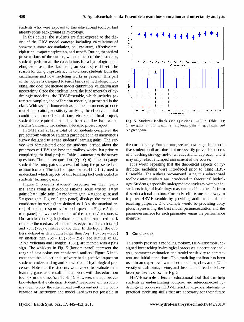
Figure 5 presents students’ responses on their learn-ing gains using a five-point ranking scale where: 1 = nogains; 2 = a little gain; 3 = moderate gain; 4 = good gain; and5 = great gain. Figure5 (top panel) displays the mean andconfidence intervals (here defined as± 3× the standard er-ror) of student responses for each question. Figure5 (bot-tom panel) shows the boxplots of the students’ responses.On each box in Fig.5 (bottom panel), the central red markrefers to the median, while the box edges are the 25th (25q)and 75th (75q) quantiles of the data. In the figure, the out-liers, defined as data points larger than 75q + 1.5 (75q− 25q)or smaller than 25q− 1.5 (75q− 25q) (seeMcGill et al.,1978; Velleman and Hoaglin, 1981), are marked with a plussign. The whiskers in Fig.5 (bottom panel) represent therange of data points not considered outliers. Figure5 indi-cates that this educational software had a positive impact onstudents understanding and knowledge of hydrological pro-cesses. Note that the students were asked to evaluate theirlearning gains as a result of their work with this educationtoolbox in the class (see Table1). However, the authors ac-knowledge that evaluating students’ responses and associat-ing them to only the educational toolbox and not to the com-bination of instruction and model used was not possible in

Fig. 5. Students feedback (see Questions 1–15 in Table1);1 = no gains; 2 = a little gain; 3 = moderate gain; 4 = good gain; and5 = great gain.

the current study. Furthermore, we acknowledge that a posi-tive student feedback does not necessarily prove the successof a teaching strategy and/or an educational approach, and itmay only reflect a lumped assessment of the course.

It is worth repeating that the theoretical aspects of hy-drologic modeling were introduced prior to using HBV-Ensemble. The authors recommend using this educationaltoolbox after students are introduced to theoretical hydrol-ogy. Students, especially undergraduate students, without ba-sic knowledge of hydrology may not be able to benefit fromthis educational toolbox. Currently, efforts are underway toimprove HBV-Ensemble by providing additional tools forteaching purposes. One example would be providing dottyplots, representing the best model parameterization and theparameter surface for each parameter versus the performancemeasure.

5 Conclusions

This study presents a modeling toolbox, HBV-Ensemble, de-signed for teaching hydrological processes, uncertainty anal-ysis, parameter estimation and model sensitivity to parame-ters and initial conditions. This modeling toolbox has beenused in an upper level watershed modeling class at the Uni-versity of California, Irvine, and the students’ feedback havebeen positive as shown in Fig.5.

HBV-Ensemble offers an educational tool that can helpstudents in understanding complex and interconnected hy-drological processes. HBV-Ensemble exposes students topractical modeling skills that are necessary for their future



Table 1.Survey questions.

As a result of your work with this education toolbox in the class, what gains did you make in each of the followings?

Q1 Hydrologic modeling in generalQ2 Water budget analysisQ3 Rainfall–runoff processes, their mathematical formulations and the required calculations to estimate the flood resulting from a

given precipitation eventQ4 The effect of evapotranspiration on rainfall–runoff processes, its mathematical formulation and the required calculationsQ5 The effect of soil moisture on rainfall–runoff processes, its mathematical formulation and the required calculationsQ6 Model calibration and ensemble simulationQ7 Sensitivity analysisQ8 Differences between empirical and physically-based parametersQ9 Enthusiasm for the subject of hydrologic modeling and analysisQ10 Confidence in performing hydrologic modeling

How each of the following aspects and attributes of the developed teaching tool contributed to your learning gains?

Q11 The use of a practical case study with actual dataQ12 The use of hands-on calculations in the lectureQ13 The fact that you could change the model parameters and see their effectsQ14 The requirement of a hydrologic modeling project using this hands-on toolbox.

careers in hydrology. The presented modeling toolbox pro-vides the opportunity for students to investigate “what-if”scenarios for initial conditions, parameters, objective func-tions, etc., and practice experiential learning.

We recommend using HBV-Ensemble after students areintroduced to theoretical aspects of hydrologic modeling.The toolbox can be used at the conclusion of an undergradu-ate hydrology class after the students have been already ex-posed to the fundamental processes; in such settings, the toolcan serve as an add-on value for early introduction of ad-vanced concepts on model uncertainty and ensemble predic-tions. HBV-Ensemble can be used for in-class lab practicesand homework assignments to improve students’ understand-ing of hydrological processes. Instructors, students and inter-ested readers can request a free copy of HBV-Ensemble foreducational purposes.

Acknowledgements.The authors would like to thank the Editorand reviewers for their constructive comments and suggestionswhich led to substantial improvements in the manuscript. We aregrateful to many colleagues and graduate students who offeredvaluable comments and suggestions for improvements. These indi-viduals include Leonardo Valerio Noto, Ali Mehran, Jeff Tuhtan,Nasrin Nasrollahi, Mehdi Rezaeian Zadeh, Naveen Duggi andMehdi Javadian. The first author acknowledges Andras Bardossy’sclasses and instruction approaches that inspired him to developeducational tools. Financial support from the United States Bureauof Reclamation (USBR) Award No. R11AP81451 to the first authorand National Science Foundation Award No. DUE-1122898 to thethird author are acknowledged.

Edited by: J. Seibert

References

AghaKouchak, A. and Habib, E.: Application of a conceptual hy-drologic model in teaching hydrologic processes, Int. J. Eng.Educ., 26, 963–973, 2010.

AghaKouchak, A., Bardossy, A., and Habib, E.: Copula-based un-certainty modeling: Application to multi-sensor precipitation es-timates, Hydrol. Process., 24, 2111–2124, 2010.

AghaKouchak, A., Bardossy, A., and Habib, E.: Extremes in aChanging Climate, Springer, Dordrecht, The Netherlands, 2012.

Bell, V. A. and Moore, R. J.: The sensitivity of catchment runoffmodels to rainfall data at different spatial scales, Hydrol. EarthSyst. Sci., 4, 653–667,doi:10.5194/hess-4-653-2000, 2000.

Bergstrom, S.: The HBV model, Computer Models of Water-shed Hydrology, in: Computer Models of Watershed Hydrology,edited by: Singh, V., Water Resources Publications, 443–476,1995.

Beven, J. and Kimberlain, T.: Tropical Cyclone Report HurricaneGustav (AL072008) 25 August–4 September 2008, Tech. rep.,National Oceanic and Atmospheric Administration (NOAA),National Hurricane Center (NHC), USA, 2009.

Beven, K.: Environmental modelling: an uncertain future?, Tay-lor & Francis, 2008.

Beven, K. and Freer, J.: Equifinality, data assimilation, and uncer-tainty estimation in mechanistic modelling of complex environ-mental systems using the GLUE methodology, J. Hydrol., 249,11–29, 2001.

Beven, K. J.: Rainfall-Runoff Modelling: The Primer, John Wileyand Sons, 2001.

Beven, K. J. and Binley, A. M.: The future role of distributed mod-els: model calibration and predictive uncertainty, Hydrol. Pro-cess., 6, 279–298, 1992.

CUAHSI: Hydrology of a Dynamic Earth: A Decadal Research Planfor Hydrologic Science, CUAHSI Science Plan draft version 7.0,USA, 2007.


http://dx.doi.org/10.5194/hess-4-653-2000


Georgakakos, K., Seo, D., Gupta, H., Schaake, J., and Butts, M.: To-wards the characterization of streamflow simulation uncertaintythrough multimodel ensembles, J. Hydrol., 298, 222–241, 2004.

Goodrich, D., Faures, J., Woolhiser, D., Lane, L., and Sorooshian,S.: Measurement and analysis of small-scale convective stormrainfall variability, J. Hydrol., 173, 283–308, 1995.

Habib, E., Ma, Y., Williams, D., Sharif, H. O., and Hossain, F.: Hy-droViz: design and evaluation of a Web-based tool for improvinghydrology education, Hydrol. Earth Syst. Sci., 16, 3767–3781,doi:10.5194/hess-16-3767-2012, 2012.

Hundecha, Y. H. and Bardossy, A.: Modeling of the effect of landuse changes on the runoff generation of a river basin throughparameter regionalization of a watershed model, J. Hydrol., 292,281–295, 2004.

McGill, R., Tukey, J., and Larsen, W.: Variations of box plots,American Stat., 32, 12–16, 1978.

Montanari, A., Shoemaker, C., and van de Giesen, N.: Introductionto special section on Uncertainty Assessment in Surface and Sub-surface Hydrology: An overview of issues and challenges, WaterResour. Res., 45, W00B00,doi:10.1029/2009WR008471, 2009.

Murphy, J., Sexton, D., Barnett, D., Jones, G., Webb, M., andCollins, M.: Quantification of modelling uncertainties in a largeensemble of climate change simulations, Nature, 430, 768–772,2004.

Nash, J. E. and Sutcliffe, J. V.: River flow forecasting through con-ceptual models, Part I,. A discussion of principles, J. Hydrol., 10,282–290, 1970.

NRC: Opportunities in the Hydrologic Sciences, National AcademyPress, Washington, D.C., 1991.

NRC: Inquiry and the National Science Education Standards: AGuide for Teaching and Learning, National Academy Press,Washington, D.C., 2000.

Obled, C., Wendling, J., and Beven, K.: The sensitivity of hydro-logical models to spatial rainfall patterns: an evaluation usingobserved data, J. Hydrol., 159, 305–333, 1994.

Pathirana, A., Gersonius, B., and Radhakrishnan, M.: Web 2.0collaboration tool to support student research in hydrol-ogy – an opinion, Hydrol. Earth Syst. Sci., 16, 2499–2509,doi:10.5194/hess-16-2499-2012, 2012.

Piani, C., Frame, D., Stainforth, D., and Allen, M.: Con-straints on climate change from a multi-thousand memberensemble of simulations, Geophys. Res. Lett., 32, L23825,doi:10.1029/2005GL024452, 2005.

Renard, B., Kavetski, D., Kuczera, G., Thyer, M., and Franks, S.:Understanding predictive uncertainty in hydrologic modeling:The challenge of identifying input and structural errors, WaterResour. Res., 46, W05521,doi:10.1029/2009WR008328, 2010.

Rodhe, A.: Physical models for classroom teaching in hydrology,Hydrol. Earth Syst. Sci., 16, 3075–3082,doi:10.5194/hess-16-3075-2012, 2012.

Rusca, M., Heun, J., and Schwartz, K.: Water management sim-ulation games and the construction of knowledge, Hydrol.Earth Syst. Sci., 16, 2749–2757,doi:10.5194/hess-16-2749-2012, 2012.

Seibert, J. and Vis, M. J. P.: Irrigania – a web-based game aboutsharing water resources, Hydrol. Earth Syst. Sci., 16, 2523–2530,doi:10.5194/hess-16-2523-2012, 2012a.

Seibert, J. and Vis, M. J. P.: Teaching hydrological modeling witha user-friendly catchment-runoff-model software package, Hy-drol. Earth Syst. Sci., 16, 3315–3325,doi:10.5194/hess-16-3315-2012, 2012b.

Shaw, S. B. and Walter, M. T.: Using comparative analysis to teachabout the nature of nonstationarity in future flood predictions,Hydrol. Earth Syst. Sci., 16, 1269–1279,doi:10.5194/hess-16-1269-2012, 2012.

Singh, V. and Woolhiser, D.: Mathematical Modeling of WatershedHydrology, J. Hydrol. Eng.-ASCE, 7, 269–343, 2002.

Thompson, S. E., Ngambeki, I., Troch, P. A., Sivapalan, M., andEvangelou, D.: Incorporating student-centered approaches intocatchment hydrology teaching: a review and synthesis, Hy-drol. Earth Syst. Sci., 16, 3263–3278,doi:10.5194/hess-16-3263-2012, 2012.

Velleman, P. and Hoaglin, D.: Applications, basics, and comput-ing of exploratory data analysis, vol. 142, Duxbury Press Boston,Boston, 1981.

Vrugt, J. A., ter Braak, C. J. F., Clark, M. P., Hyman, J. M.,and Robinson, B. A.: Treatment of input uncertainty in hy-drologic modeling: Doing hydrology backward with Markovchain Monte Carlo simulation, Water Resour Res., 44, W00B09,doi:10.1029/2007WR006720, 2008.

Wagener, T.: Evaluation of catchment models, Hydrol. Process., 17,3375–3378, 2003.

Wagener, T., Wheater, H., and Gupta, H.: Rainfall-runoff modellingin gauged and ungauged catchments, Imperial College Press,London, UK, 2004.

Wagener, T., Sivapalan, M., Troch, P. A., McGlynn, B. L., Har-man, C. J., Gupta, H. V., Kumar, P., Rao, P. S. C., Basu, N. B.,and Wilson, J. S.: The future of hydrology: An evolving sci-ence for a changing world, Water Resour. Res., 46, W05301,doi:10.1029/2009WR008906, 2010.

Wagener, T., Kelleher, C., Weiler, M., McGlynn, B., Gooseff, M.,Marshall, L., Meixner, T., McGuire, K., Gregg, S., Sharma, P.,and Zappe, S.: It takes a community to raise a hydrologist: theModular Curriculum for Hydrologic Advancement (MOCHA),Hydrol. Earth Syst. Sci., 16, 3405–3418,doi:10.5194/hess-16-3405-2012, 2012.

Wheater, H. S., Jakeman, A. J., and Beven, K. J.: Progress and di-rections in rainfall-runoffmodelling, in: Modelling change in en-vironmental systems, edited by: Jakeman, A. J., Beck, M. B., andMcAleer, M. J., Wiley, 1993.

Wood, A., Maurer, E., Kumar, A., and Lettenmaier, D.: Long-range experimental hydrologic forecasting for the easternUnited States, J. Geophys. Res.-Atmos., 107, ACL6-1-15,doi:10.1029/2001JD000659, 2002.

Young, P.: Advances in real-time flood forecasting, Philos. T. Roy.Soc. Lond. A, 360, 1433–1450, 2002.



http://dx.doi.org/10.1029/2009WR008471


http://dx.doi.org/10.1029/2005GL024452

http://dx.doi.org/10.1029/2009WR008328












http://dx.doi.org/10.1029/2007WR006720

http://dx.doi.org/10.1029/2009WR008906



http://dx.doi.org/10.1029/2001JD000659

an educational model for ensemble streamﬂow...

Documents