An Educational Tool for

the Material Point

Method MAE 8085 Final Report

Jessica Bales

M.S. Candidate

Mechanical Engineering Department

Advisor: Dr. Zhen Chen

C.W. LaPierre Professor

Civil Engineering Department

May 2014

The undersigned, appointed by the dean of the Graduate School, have examined the

report entitled

AN EDUCATIONAL TOOL FOR THE

MATERIAL POINT METHOD

presented by Jessica Bales,

a candidate for the degree of Master of Science in Mechanical and Aerospace

Engineering

and hereby certify that, in their opinion, it is worthy of acceptance.

Professor Zhen Chen

Professor Vellore Gopalaratnam

Professor P. Frank Pai

ii

Acknowledgements

I would like to thank my advisor, Dr. Zhen Chen for his instruction and support

throughout this project. Also, Shan Jiang and Bin Wang for their guidance in the

algorithm of the program. I would also like to thank Hao Peng and Glenn Smith for their

MATLAB programming advice.

iii

Abstract

The Material Point Method (MPM), a particle method designed for simulating

large deformations and the interactions between different material phases, has

demonstrated its potential in modern engineering applications. To promote integrated

research and educational activities, a user-friendly educational tool in MATLAB is

needed. In this report, the theory and algorithm of this educational tool are documented.

To validate the effectiveness of the tool, both one- and two-dimensional wave and impact

problems are solved using a linear elastic model. The numerical results are then

compared and verified against available analytical solutions, and the numerical solutions

from an existing one-dimensional MPM code and ABAQUS, a Finite Element Method

based program.

iv

Table of Contents

1. Acknowledgements ..............................................................................................ii

2. Abstract ................................................................................................................iii

3. Table of Tables ....................................................................................................v

4. Table of Figures ...................................................................................................vi

5. Introduction ..........................................................................................................1

6. Previous Work .....................................................................................................3

7. Theory ..................................................................................................................4

8. Algorithm .............................................................................................................9

9. Validation .............................................................................................................12

10. Demonstration ......................................................................................................16

11. Conclusion ...........................................................................................................18

12. References ............................................................................................................19

13. Appendices

A. Tables .......................................................................................................20

B. Figures......................................................................................................27

C. MATLAB Code .......................................................................................36

D. Sample Input File .....................................................................................41

v

Table of Tables

Table 1. Material properties of bar extension .....................................................................20

Table 2. Comparison of one- and two-dimensional bar extension .....................................20

Table 3. Material properties of bar collision.......................................................................21

Table 4. Comparison of one- and two-dimensional bar collision .......................................22

Table 5. Material properties of beam bending ....................................................................23

Table 6. Comparison of 20x8 beam with one point per cell ...............................................23

Table 7. Comparison of 10x4 beam with one point per cell ...............................................24

Table 8. Comparison of 10x4 beam with four points per cell ............................................25

Table 9. Material properties of disc collision .....................................................................25

Table 10. Comparison of the distance between two nodes .................................................26

Table 11. Material properties of projectile .........................................................................26

vi

Table of Figures

Figure 1. Longitudinal stress in one-dimensional bar wavecase ........................................27

Figure 2. Longitudinal stress in two-dimensional bar wavecase ........................................27

Figure 3. Material point locations during a two-dimensional bar collision ........................28

Figure 4. Longitudinal stress in one-dimensional bar collision ..........................................28

Figure 5. Longitudinal stress in two-dimensional bar collision ..........................................29

Figure 6. Initial locations in a disc collision .......................................................................29

Figure 7. Distance between two nodes on a larger mesh ....................................................30

Figure 8. Configuration of projectile collision ...................................................................30

Figure 9. Initial locations of a projectile in uniaxial stress .................................................31

Figure 10. Longitudinal stress in a projectile collision in uniaxial stress ...........................31

Figure 11. Transverse stress in a projectile collision in uniaxial stress ..............................32

Figure 12. Stresses at point A in a projectile collision in uniaxial stress ...........................32

Figure 13. Stresses at point B in a projectile collision in uniaxial stress ............................33

Figure 14. Initial locations of a projectile in uniaxial strain ...............................................33

Figure 15. Longitudinal stress in a projectile collision in uniaxial strain ...........................34

Figure 16. Transverse stress in a projectile collision in uniaxial strain ..............................34

Figure 17. Stresses at point A in a projectile collision in uniaxial strain ...........................35

Figure 18. Stresses at point B in a projectile collision in uniaxial strain ............................35

- 1 -

Introduction

The Material Point Method (MPM) is a numerical method for solving problems in

solid mechanics. It is considered a “meshless” spatial discretization strategy because the

continuum is not mapped with a rigid mesh, but is divided into material points that move

along an arbitrary background mesh that does not hold the state variables. The material

points, which hold these state variables between computational iterations, are updated

using the background nodes that are reset at the end of each iteration. The Material Point

Method is based on the amalgamation of the background mesh and the material points,

taking advantage of both the Eulerian and Lagrangian descriptions of motion.

In solid mechanics, the Material Point Method shows promise in several areas to

be more effective than the better known, and more widely used, Finite Element Method

(FEM). Because the material points store the mass, velocity, and other state variables

between time steps, the remeshing of the background does not produce errors. In FEM,

large deformations can result in errors because of the remeshing of the solid itself. This

crucial difference allows MPM to successfully model large deformations, penetration,

collision, crack propagation, and granular flow. It can also handle multiphase problems,

with different constitutive relations for the different phases, e.g. solid, liquid, or gas.

Wave propagation, thermal diffusion, and other multiphysics situations can also be

evaluated using the MPM.

Despite its many possibilities, MPM has not yet been used in a commercial code.

In order to introduce students to MPM at the University of Missouri, a straightforward

two-dimensional code is needed. Although a FORTRAN code already exists, a program

- 2 -

using MATLAB will be more useful because of the simpler language and more compact

structure. Beyond an introductory educational tool, this code may also be extended to

research in other areas, like plastic collisions and crack propagation. This MPM code can,

therefore, be used as an educational tool in many areas within the University of Missouri.

The purpose of this report is to introduce and validate the two-dimensional

algorithm and MATLAB code used to create the MPM program. The previous work and

theory behind the Material Point Method are necessary for an understanding of the

program. To verify the validity of the program, several cases are investigated and the

MPM results are compared to the results from existing numerical techniques. A final

demonstration of the capability of the MPM code is included to suggest further uses for

the Material Point Method.

- 3 -

Previous Work

This key combination was first theorized in the 1950’s in the Particle-in-Cell

(PIC) method, which was developed to trace the movement of supersonic fluid flow [4].

In this approach, each particle was assigned mass, but not velocity or energy. With the

advent of more powerful computers, the first PIC code, called Fluid-Implicit Particle

(FLIP), was developed in 1986 [2]. In the 1990’s, the Material Point Method was

developed in order to solve solid mechanic problems using an Eulerian background mesh

and Lagrangian particles [7]. Subsequent applications, like granular flow [1] and crack

propagation [5], show the wide range of possibilities for the Material Point Method. Most

recently, MPM was used to animate snow in a full-length motion picture, Frozen, which

has greatly increased the recognition of this type of numerical method [6].

- 4 -

Theory

Like the Finite Element Method, and other discretization procedures, MPM is

used to numerically solve the governing differential equations of a particular continuum.

These are derived from the equation of mass conservation,

(1)

and the equation for the conservation of momentum,

(2)

where is the mass density vector, is the velocity vector, is the acceleration vector,

is the Cauchy stress tensor, and is the specific body force.

In MPM, the continuum is discretized into material points. Each point carries all

the same properties as the original volume of the continuum that it represents. Despite

any deformation of the continuum as a whole, each material point maintains those

properties, including mass. Because they have constant mass throughout the simulation,

the material points fulfill the requirements of the conservation of mass equation. The

location of each point is recorded at the end of every time step, which follows the

Lagrangian description of motion.

Alternatively, the background mesh follows the Eulerian description of motion.

Within each iteration, the mesh deforms based on the movement of the particles during

the same time step. This method provides information on the motion of all the particles at

one time, following the Eulerian approach. The relationship between the motion of the

particles and of the nodes in the background mesh is established through the weak form

of the conservation of momentum equation,

(3)

- 5 -

where w is the test function, assumed to be zero on the boundary with prescribed

displacement; ss is specific stress ; is the current configuration of the

continuum; Sc is that part of the boundary with a prescribed traction; and ρ is the mass

density. Because this is a numerical technique, and the continuum is described with a

finite number of material points, the mass density may be written as a sum,

(4)

where Mp is the particle mass and δ is the Dirac delta function with the dimension of the

inverse of volume.

By substituting Eq. (4) into Eq. (3), the weak form becomes discrete,

(5)

where h is the thickness. The gradient terms may only be calculated through a

background mesh. The background mesh is composed of 2-node cells for a one-

dimensional case and 4-node cells for a two-dimensional case. As in FEM, shape

functions are used to describe locations in the local coordinate system. The shape

functions in one-dimension are

(6a)

(6b)

where ξ is the coordinate of the material point in the x-direction. In two-dimensions, the

shape functions are

- 6 -

(7a)

(7b)

(7c)

(7d)

where ξ and η are the coordinates of the material point along the x- and y-directions,

respectively. Relating the material points and nodes can, therefore, be performed through

the shape functions,

(8a)

(8b)

(8c)

(8d)

where Nn is the total number of nodes in the background mesh and Ni is the shape

function. In two-dimensions, Ni corresponds to the four nodes related to each material

point (i = 1, 2, 3, 4).

Substituting Eqs. (8c) and (8d) into Eq. (5) yields

(9)

where the mass matrix is

(10)

- 7 -

and the specific traction is

(11)

The specific body force is

(12)

Because the weight function is arbitrary, it may be factored from Eq. (9), leaving

(13)

The internal force vector is

(14)

where G is the derivative of the shape function evaluated at a particular particle location.

The external force is

(15)

In each time iteration, the state variables are mapped between the nodes and the

particles and Eq. (13) is solved. The total time of the simulation is arbitrary and specified

by the user, but the time step is determined by the wave speed of the smallest cell. The

largest time step that may be used is

(16)

where L is the length of the cell along the wave direction and the wave speed is

(17)

- 8 -

The central processing unit, described in the algorithm, is repeated for every time step of

this size.

- 9 -

Algorithm

Preprocessor

1. The initial background mesh is established. Because remeshing is unnecessary for

the validation problems, this arbitrary mesh is used throughout each problem.

2. The continuum body is discretized into material points, which carry the property

materials of the surrounding area.

3. All the state variables are initialized.

4. The control parameters are established.

Central Processing Unit [3]

1. Map from the particles to the nodes containing those particles.

Map the mass from the particles to the corresponding nodes,

(18)

where is the mass of node i at time t, is the mass of the particle, is the

shape function for node i at the particle location, , at time t.

Map the momentum from the particles to the corresponding nodes,

(19)

where is the nodal momentum at node i and time t, and

is the

particle momentum at time t.

Calculate internal forces at the nodes,

(20)

- 10 -

where is the internal force at node i and time t,

is the shape

gradient for node i at particle location ,

is the particle stress at time t, and

is the particle density at time t.

2. Apply essential and natural boundary conditions to the nodes and compute nodal

force vector,

(21)

where is the total force at node i and time t, and

is the external, or

applied, force at node i and time t.

3. Update the momenta at the nodes,

(22)

4. Map from the nodes to the particles within those nodes.

Map the nodal accelerations back to the particle,

(23)

Map nodal velocities back to the particles

(24)

Compute the particle velocity,

(25)

Compute the particle position,

(26)

5. Map particle momenta to the nodes,

(27)

6. Find the updated nodal velocities,

- 11 -

(28)

7. Apply essential boundary conditions to the grid nodes of the cells containing

boundary particles.

8. Find the current gradient of particle velocity and the strain gradient,

(29)

(30)

9. Find stress gradient,

(31)

where T is the compliance matrix from the constitutive model.

10. Identify which grid cell each particle belongs to, and update the natural coordinates

of the particle.

11. If the final time has not been reached, return to Step 1.

Post Processor

1. Divide the total time duration by the number of iterations. Divide the continuum

into manageable sections.

2. Graph particle location and stress versus time in order to verify the results.

- 12 -

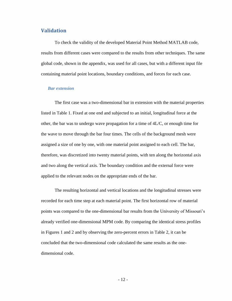
Validation

To check the validity of the developed Material Point Method MATLAB code,

results from different cases were compared to the results from other techniques. The same

global code, shown in the appendix, was used for all cases, but with a different input file

containing material point locations, boundary conditions, and forces for each case.

Bar extension

The first case was a two-dimensional bar in extension with the material properties

listed in Table 1. Fixed at one end and subjected to an initial, longitudinal force at the

other, the bar was to undergo wave propagation for a time of 4L/C, or enough time for

the wave to move through the bar four times. The cells of the background mesh were

assigned a size of one by one, with one material point assigned to each cell. The bar,

therefore, was discretized into twenty material points, with ten along the horizontal axis

and two along the vertical axis. The boundary condition and the external force were

applied to the relevant nodes on the appropriate ends of the bar.

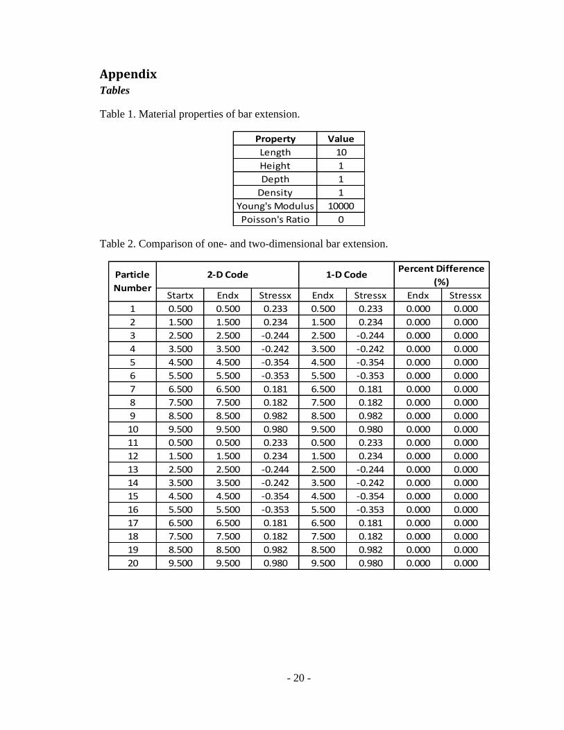
The resulting horizontal and vertical locations and the longitudinal stresses were

recorded for each time step at each material point. The first horizontal row of material

points was compared to the one-dimensional bar results from the University of Missouri’s

already verified one-dimensional MPM code. By comparing the identical stress profiles

in Figures 1 and 2 and by observing the zero-percent errors in Table 2, it can be

concluded that the two-dimensional code calculated the same results as the one-

dimensional code.

- 13 -

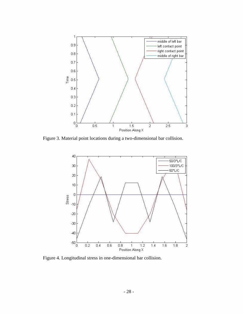
Bar collision

Table 3 describes the material properties of a two-dimensional bar collision

problem. Here, two bars, each with the listed material properties, were placed one unit

apart and given an initial velocity toward each other. The initial velocity was applied at

the material points. They collided elastically, guaranteed by an appropriate constitutive

model and compliance matrix in Eq. 31, and then rebounded. The background mesh was

again one by one unit, with one material point in each cell. There was a total of 40

material points, 20 in each bar.

The horizontal and vertical location components and longitudinal stresses were

again compared to the results from the one-dimensional MPM code. Figures 4-5 and

Table 4 reveal complete agreement between the two different codes.

Beam bending

The third case was a cantilever beam subjected to bending. The beam, with

material properties listed in Table 5, was fixed at one end and subjected to a transverse

load at the other end. Both the boundary condition and the load were applied to the

appropriate background nodes. In this case, there were three different material point and

background mesh configurations used. The first had a background mesh with a size of

one by one, with one particle per cell. Another case fit four material points into one cell,

with the same background mesh. The last used a background mesh that was 0.5 by 0.5

units, with one particle per cell. The second tests the effect of more nodes in each cell,

while the third tests the effect of smaller cells. In these cases, it was necessary to keep the

displacements very small, so that the material points do not cross into other cells. This is

- 14 -

because the force is applied to a node that needs to maintain contact with a material point

to have any effect and because the code cannot handle a material point on the boundary

line. If this happened, the code would not be able to place the material point within a cell

in order to map to the nodes.

These small deformations were compared to the results obtained by solving the

same problem in ABAQUS, a Finite Element Method based commercial program. The

model was composed of 4-node bilinear plane stress elements, with reduced integration

and hourglass control. In ABAQUS, the displacements are calculated only at the nodes of

the mesh, so the mesh was designed with a node at the location of each material point.

This results in a mesh that is more fine than the MPM background mesh, which could

account for some discrepancies. The percent errors between the horizontal and vertical

locations were calculated in Tables 6-8, but the errors in the particles furthest from the

fixed end were of interest. These particles experienced the most displacement. In the first

case, the average percent error in the vertical direction for these material points was

4.12%. Increasing the number of nodes per cell decreased the percent error to 2.42%.

Refining the background mesh decreased the error to 1.51%.

Disc collision

The next case tested was the collision of two discs. For later comparison, it was

first computed using ABAQUS. The node locations assigned in this program, using four-

node linear tetrahedal elements, were transferred into MATLAB to be used as the

material point locations. Although it was modeled in three-dimensions in ABAQUS, the

depth was the same in each method. Two different background meshes were used with

- 15 -

the same material point configuration: a more coarse, 40 by 40 cell mesh and a more

refined, 50 by 50 mesh.

The distance between two different nodes was recorded at regular intervals in both

the MPM code and in ABAQUS. The comparisons between the MPM and ABAQUS

results are shown in Table 10 and in Figure 7. The average percent difference in the

distance between the nodes was 10.15% for the coarse mesh and 4.12% for the finer

mesh. However, when the mesh was made more fine than 50 by 50, the simulation could

not complete the collision because there were cells within the discs that did not contain

any material points. To refine the mesh, therefore, more material points would be

required for the same disc size.

- 16 -

Demonstration

To demonstrate the capability of the MPM MATLAB code to simulate uniaxial

strain and uniaxial stress, two cases in which a projectile strikes an object were examined.

The projectile and the object had the same material properties, listed in Table 12 and the

configurations in Figures 8, 9, and 14. The flyer material points had an initial velocity of

one toward the object. First, the projectile struck the smaller end, simulating a uniaxial

stress case, which is similar to the bar impact problem discussed earlier. Like the bar

impact or extension cases, the stress wave can be observed moving through the

continuum at different times in Figures 10-11. The longitudinal and transverse stresses

reported were collected from the second row of material points from the bottom of the

‘bar’. The stresses at two different points, the middle of the ‘bar’ and the middle of the

‘plate’ part of the continuum, can be seen in Figures 12-13.

Next, the projectile was simulated striking the larger end, similar to a uniaxial

strain case, like a plate impact. Figures 15-16 show the stress wave moving through the

solid at the same times as the first projectile case. In comparison to the first case, the

longitudinal stresses are very similar. The transverse stresses, however, are more

pronounced than in the first case, due to the change in geometry. Figures 17-18 show the

longitudinal and transverse stress values at the same two points as in the first case. When

these are compared to the first case, it can be observed that nearly all the stresses in the

first case have a greater magnitude than those of the second case. The only exception is

the transverse stress at point B, which is expected because of the inability of the ‘plate’ to

distribute stress in the transverse direction. This behavior is described by uniaxial strain.

- 17 -

The results of these two cases qualitatively support the effective simulation of uniaxial

stress and strain by the MPM code.

- 18 -

Conclusion

Based on the low, or at least decreasing, percent errors in the first validation

cases, this Material Point Method MATLAB code is an effective tool for solving these

problems. The straightforward MATLAB algorithm and descriptive comments make this

code valuable in educating and introducing students to the Material Point Method.

Further, this base code could be extended to solve more complicated problems, such as

plastic collision and crack propagation, through remeshing techniques and more

comprehensive constitutive models. New input files may be easily created to incorporate

these methods.

Some improvements to this code may be made. The shape functions may be

expressed in global terms, which would allow problems, like the beam bending, to cross

cell boundaries. For many of these validation cases, the ideal background mesh size,

material point configuration, and their relationship were not fully investigated. Such an

investigation could lead to improved results in these and more complex problems.

- 19 -

References [1] Bardenhagen, S.G., J.U. Brackbill, and D. Sulsky. "The material-point method for

granular materials." Computer Methods in Applied Mechanics and Engineering

187: 529-541.

[2] Brackbill, J.U., D.B. Kothe, and H.M. Ruppel. "FLIP: A Low-Dissipation,

Particle-In-Cell Method for Fluid Flow." Computer Physics Communications 48

(1988): 25-38.

[3] Chen, Brannon. “An Evaluation of the Material Point Method.” Sandia National

Laboratories. (2002). Print.

[4] Harlow, F.H. (1964), “The Particle-in-Cell Computing Method for Fluid

Dynamics in Fundamental Methods in Hydrodynamics,” Experimental

Arithmetic, High-Speed Computations and Mathematics, Edited by B. Alder, S.

Fernbach and M.Rotenberg, Academic Press, pp. 319-345.

[5] Nairn, John A, "Material Point Method Calculations with Explicit Cracks,"

Computer Modeling in Eng. & Sci., 4, 649-664 (2003).

[6] Stomakhin, Schroeder, Chai, Teran, Selle (August 2013). "A material point

method for snow simulation". Walt Disney Animation Studios.

[7] Sulsky, D., Zhou, S.J., and Schreyer, H.L. (1995), “Application of a Particle-in-

Cell Method to Solid Mechanics,” Computer Physics Communications, Vol. 87,

pp. 236-252.

- 20 -

Appendix Tables

Table 1. Material properties of bar extension.

Property Value

Length 10

Height 1

Depth 1

Density 1

Young's Modulus 10000

Poisson's Ratio 0

Table 2. Comparison of one- and two-dimensional bar extension.

Startx Endx Stressx Endx Stressx Endx Stressx

1 0.500 0.500 0.233 0.500 0.233 0.000 0.000

2 1.500 1.500 0.234 1.500 0.234 0.000 0.000

3 2.500 2.500 -0.244 2.500 -0.244 0.000 0.000

4 3.500 3.500 -0.242 3.500 -0.242 0.000 0.000

5 4.500 4.500 -0.354 4.500 -0.354 0.000 0.000

6 5.500 5.500 -0.353 5.500 -0.353 0.000 0.000

7 6.500 6.500 0.181 6.500 0.181 0.000 0.000

8 7.500 7.500 0.182 7.500 0.182 0.000 0.000

9 8.500 8.500 0.982 8.500 0.982 0.000 0.000

10 9.500 9.500 0.980 9.500 0.980 0.000 0.000

11 0.500 0.500 0.233 0.500 0.233 0.000 0.000

12 1.500 1.500 0.234 1.500 0.234 0.000 0.000

13 2.500 2.500 -0.244 2.500 -0.244 0.000 0.000

14 3.500 3.500 -0.242 3.500 -0.242 0.000 0.000

15 4.500 4.500 -0.354 4.500 -0.354 0.000 0.000

16 5.500 5.500 -0.353 5.500 -0.353 0.000 0.000

17 6.500 6.500 0.181 6.500 0.181 0.000 0.000

18 7.500 7.500 0.182 7.500 0.182 0.000 0.000

19 8.500 8.500 0.982 8.500 0.982 0.000 0.000

20 9.500 9.500 0.980 9.500 0.980 0.000 0.000

Particle

Number

Percent Difference

(%)1-D Code2-D Code

- 21 -

Table 3. Material properties of bar collision.

Property Value

Length 1

Height 1

Depth 1

Density 1

Young's Modulus 10000

Poisson's Ratio 0

- 22 -

Table 4. Comparison of one- and two-dimensional bar collision.

Startx Endx Stressx Endx Stressx Endx Stressx

1 0.100 0.142 -46.338 0.142 -46.338 0.000 0.000

2 0.300 0.341 -11.239 0.341 -11.239 0.000 0.000

3 0.500 0.541 18.928 0.541 18.928 0.000 0.000

4 0.700 0.742 -28.449 0.742 -28.449 0.000 0.000

5 0.900 0.942 12.244 0.942 12.244 0.000 0.000

6 2.100 2.058 12.244 2.058 12.244 0.000 0.000

7 2.300 2.258 -28.449 2.258 -28.449 0.000 0.000

8 2.500 2.459 18.928 2.459 18.928 0.000 0.000

9 2.700 2.659 -11.239 2.659 -11.239 0.000 0.000

10 2.900 2.858 -46.338 2.858 -46.338 0.000 0.000

11 0.100 0.142 -46.338 0.142 -46.338 0.000 0.000

12 0.300 0.341 -11.239 0.341 -11.239 0.000 0.000

13 0.500 0.541 18.928 0.541 18.928 0.000 0.000

14 0.700 0.742 -28.449 0.742 -28.449 0.000 0.000

15 0.900 0.942 12.244 0.942 12.244 0.000 0.000

16 2.100 2.058 12.244 2.058 12.244 0.000 0.000

17 2.300 2.258 -28.449 2.258 -28.449 0.000 0.000

18 2.500 2.459 18.928 2.459 18.928 0.000 0.000

19 2.700 2.659 -11.239 2.659 -11.239 0.000 0.000

20 2.900 2.858 -46.338 2.858 -46.338 0.000 0.000

21 0.100 0.142 -46.338 0.142 -46.338 0.000 0.000

22 0.300 0.341 -11.239 0.341 -11.239 0.000 0.000

23 0.500 0.541 18.928 0.541 18.928 0.000 0.000

24 0.700 0.742 -28.449 0.742 -28.449 0.000 0.000

25 0.900 0.942 12.244 0.942 12.244 0.000 0.000

26 2.100 2.058 12.244 2.058 12.244 0.000 0.000

27 2.300 2.258 -28.449 2.258 -28.449 0.000 0.000

28 2.500 2.459 18.928 2.459 18.928 0.000 0.000

29 2.700 2.659 -11.239 2.659 -11.239 0.000 0.000

30 2.900 2.858 -46.338 2.858 -46.338 0.000 0.000

31 0.100 0.142 -46.338 0.142 -46.338 0.000 0.000

32 0.300 0.341 -11.239 0.341 -11.239 0.000 0.000

33 0.500 0.541 18.928 0.541 18.928 0.000 0.000

34 0.700 0.742 -28.449 0.742 -28.449 0.000 0.000

35 0.900 0.942 12.244 0.942 12.244 0.000 0.000

36 2.100 2.058 12.244 2.058 12.244 0.000 0.000

37 2.300 2.258 -28.449 2.258 -28.449 0.000 0.000

38 2.500 2.459 18.928 2.459 18.928 0.000 0.000

39 2.700 2.659 -11.239 2.659 -11.239 0.000 0.000

40 2.900 2.858 -46.338 2.858 -46.338 0.000 0.000

Particle

Number

Percent Difference

(%)1-D Code2-D Code

- 23 -

Table 5. Material properties of beam bending.

Property Value

Length 10

Height 4

Depth 1

Density 1

Young's Modulus 10000

Poisson's Ratio 0.3

Table 6. Comparison 20x8 beam with one point per cell.

Endx Endy Endx Endy Endx Endy

1 0.25 0.24 0.25 0.25 0.25 3.87

2 0.75 0.24 0.75 0.25 0.18 1.96

3 1.26 0.24 1.25 0.24 0.14 0.10

4 1.76 0.24 1.76 0.24 0.09 1.41

5 2.26 0.24 2.26 0.24 0.02 0.60

6 2.77 0.24 2.77 0.24 0.04 1.57

7 3.27 0.25 3.28 0.24 0.10 2.71

8 3.78 0.25 3.78 0.25 0.10 2.11

9 4.28 0.27 4.28 0.26 0.00 1.66

10 4.79 0.28 4.79 0.27 0.01 1.15

11 5.29 0.29 5.30 0.29 0.04 1.00

12 5.80 0.30 5.80 0.30 0.09 1.28

13 6.30 0.32 6.31 0.31 0.09 1.16

14 6.80 0.34 6.81 0.33 0.11 1.00

15 7.30 0.35 7.31 0.35 0.11 0.39

16 7.81 0.37 7.81 0.37 0.10 0.18

17 8.31 0.39 8.32 0.39 0.11 0.87

18 8.81 0.41 8.82 0.42 0.12 1.93

19 9.31 0.43 9.32 0.45 0.13 3.62

20 9.81 0.46 9.82 0.49 0.11 6.07

40 9.79 0.95 9.80 0.97 0.05 2.03

60 9.77 1.45 9.78 1.47 0.04 1.22

80 9.76 1.94 9.76 1.96 0.00 0.82

100 9.74 2.44 9.74 2.46 0.02 0.60

120 9.72 2.94 9.72 2.96 0.03 0.49

140 9.70 3.44 9.70 3.46 0.07 0.45

160 9.68 3.94 9.67 3.96 0.09 0.41

Particle

Number

Matlab Abaqus % Error

- 24 -

Table 7. Comparison 10x4 beam with one point per cell.

Endx Endy Endx Endy Endx Endy

1 0.51 0.51 0.51 0.51 0.19 0.08

2 1.54 0.54 1.54 0.54 0.19 1.04

3 2.55 0.59 2.56 0.58 0.15 1.50

4 3.56 0.64 3.57 0.63 0.19 0.92

5 4.57 0.69 4.58 0.69 0.28 0.33

6 5.57 0.75 5.59 0.76 0.30 1.01

7 6.58 0.81 6.59 0.84 0.29 3.07

8 7.57 0.87 7.60 0.92 0.32 4.89

9 8.57 0.93 8.60 0.99 0.31 6.22

10 9.57 1.00 9.60 1.08 0.26 8.10

11 0.50 1.50 0.50 1.50 0.14 0.02

12 1.51 1.54 1.51 1.53 0.30 0.44

13 2.52 1.58 2.52 1.57 0.15 0.58

14 3.52 1.64 3.52 1.63 0.11 0.45

15 4.52 1.69 4.53 1.69 0.11 0.09

16 5.52 1.75 5.53 1.76 0.08 0.29

17 6.52 1.81 6.53 1.83 0.06 1.20

18 7.52 1.87 7.53 1.91 0.05 2.10

19 8.52 1.93 8.52 1.99 0.04 2.96

20 9.52 1.99 9.52 2.07 0.03 3.92

21 0.50 2.50 0.50 2.50 0.32 0.05

22 1.49 2.54 1.49 2.53 0.01 0.35

23 2.48 2.58 2.48 2.57 0.01 0.35

24 3.48 2.63 3.48 2.63 0.01 0.23

25 4.47 2.69 4.47 2.69 0.01 0.01

26 5.47 2.75 5.47 2.76 0.04 0.24

27 6.47 2.81 6.46 2.83 0.10 0.73

28 7.46 2.87 7.45 2.91 0.11 1.27

29 8.46 2.93 8.45 2.99 0.12 1.90

30 9.46 2.98 9.45 3.06 0.10 2.59

31 0.48 3.48 0.49 3.51 1.10 0.62

32 1.46 3.54 1.47 3.53 0.01 0.29

33 2.45 3.59 2.44 3.58 0.14 0.28

34 3.43 3.63 3.43 3.63 0.23 0.15

35 4.42 3.69 4.41 3.69 0.20 0.01

36 5.42 3.75 5.40 3.76 0.24 0.24

37 6.41 3.81 6.39 3.83 0.33 0.47

38 7.41 3.87 7.38 3.91 0.36 0.91

39 8.41 3.93 8.38 3.98 0.36 1.35

40 9.41 3.98 9.37 4.06 0.38 1.88

% DifferenceAbaqusMatlabParticle

Number

- 25 -

Table 8. Comparison of 10x4 beam with four points per cell.

Endx Endy Endx Endy Endx Endy

19 9.37 0.81 9.37 0.87 0.04 7.18

20 9.87 0.87 9.87 0.81 0.01 7.92

39 9.32 1.30 9.33 1.35 0.09 3.89

40 9.82 1.35 9.83 1.30 0.09 3.21

59 9.29 1.80 9.29 1.84 0.03 2.43

60 9.79 1.84 9.79 1.80 0.03 2.01

79 9.26 2.30 9.25 2.34 0.04 1.73

80 9.76 2.33 9.75 2.30 0.04 1.64

99 9.22 2.79 9.21 2.83 0.05 1.41

100 9.72 2.83 9.71 2.79 0.05 1.41

119 9.18 3.29 9.18 3.33 0.05 1.15

120 9.68 3.33 9.68 3.29 0.03 1.20

139 9.15 3.79 9.14 3.82 0.04 0.89

140 9.64 3.83 9.64 3.79 0.00 1.04

159 9.11 4.29 9.11 4.32 0.01 0.76

160 9.61 4.33 9.61 4.29 0.06 0.93

Particle

Number

Matlab Abaqus Percent Difference

Table 9. Material properties of disc collision.

Property Value

Diameter 10

Depth 1

Density 1

Young's Modulus 10000

Poisson's Ratio 0

- 26 -

Table 10. Comparison of the distance between two nodes on a smaller mesh.

Fine Mesh Coarse Mesh Fine Mesh Coarse Mesh Fine Mesh Coarse Mesh

0 51.1753 51.1753 51.1753 51.1753 0.00 0.00

1 48.3475 48.3475 48.3475 48.3475 0.00 0.00

2 45.5197 45.5197 45.5196 45.5196 0.00 0.00

3 42.6920 42.6920 42.6921 42.6921 0.00 0.00

4 39.8645 39.8645 39.8648 39.8648 0.00 0.00

5 37.0370 37.0370 37.0375 37.0375 0.00 0.00

6 34.2098 34.2098 34.2105 34.2105 0.00 0.00

7 31.3827 31.3827 31.3836 31.3836 0.00 0.00

8 28.5559 28.5559 28.5567 28.5567 0.00 0.00

9 25.7295 25.7295 25.7295 25.7295 0.00 0.00

10 22.9036 22.9036 22.9024 22.9024 0.00 0.00

11 20.0783 20.0783 20.0761 20.0761 0.01 0.01

12 17.2541 17.2541 17.2507 17.2507 0.02 0.02

13 14.4312 14.7954 14.4271 14.4271 0.03 2.55

14 13.9056 16.6365 11.6064 11.6064 19.81 43.34

15 16.3340 19.1604 13.6116 13.6116 20.00 40.77

16 18.7642 21.7238 16.2638 16.2638 15.37 33.57

17 21.1618 24.2704 18.9169 18.9169 11.87 28.30

18 23.6411 26.8482 21.5730 21.5730 9.59 24.45

19 25.9572 29.3990 24.2343 24.2343 7.11 21.31

20 27.6159 31.9452 26.8896 26.8896 2.70 18.80

Distance in Matlab Distance in Abaqus Percent Error (%)Time

Table 11. Material properties of projectile.

Property Value

Depth 1

Density 1

Young's Modulus 10000

Poisson's Ratio 0.3

- 27 -

Figures

Figure 1. Longitudinal stress in one-dimensional bar wavecase.

Figure 2. Longitudinal stress in two-dimensional bar wavecase.

- 28 -

Figure 3. Material point locations during a two-dimensional bar collision.

Figure 4. Longitudinal stress in one-dimensional bar collision.

- 29 -

Figure 5. Longitudinal stress in two-dimensional bar collision.

Figure 6. Initial locations in a disc collision.

- 30 -

Figure 7. Distance between two nodes on a larger mesh.

Figure 8. Configuration of projectile collision.

0

10

20

30

40

50

60

0 5 10 15 20

Dis

tan

ce B

etw

ee

n T

wo

No

de

s

Time

Abaqus

MPM Fine Mesh

MPM Coarse Mesh

- 31 -

Figure 9. Initial locations of a projectile in uniaxial stress.

Figure 10. Longitudinal stress in a projectile collision in uniaxial stress at different times.

- 32 -

Figure 11. Transverse stress in a projectile collision in uniaxial stress at different times.

Figure 12. Stresses at point A in a projectile collision in uniaxial stress.

- 33 -

Figure 13. Stresses at point B in a projectile collision in uniaxial stress.

Figure 14. Initial locations of a projectile in uniaxial strain.

- 34 -

Figure 15. Longitudinal stress in a projectile collision in uniaxial strain at different times.

Figure 16. Transverse stress in a projectile collision in uniaxial strain at different times.

- 35 -

Figure 17. Stresses at point A in a projectile collision in uniaxial strain.

Figure 18. Stresses at point B in a projectile collision in uniaxial strain.

- 36 -

MATLAB Code

% Clear previous

close all;

clear all;

fid = fopen('filename.txt'); % read from text file named "filename"

% Element information

rho = fscanf(fid,'%d',1); % density

ys = fscanf(fid,'%d',1); % Young's modulus

D = fscanf(fid,'%d',1); % depth of element

L = fscanf(fid,'%d',1); % length of element

nu = fscanf(fid,'%f',1); % Poisson's ratio

vnot = fscanf(fid,'%d',1); % initial velocity value (may not be needed)

d = [ys/(1-(nu^2)) ys*nu/(1-(nu^2)) 0;...

ys*nu/(1-(nu^2)) ys/(1-(nu^2)) 0;...

0 0 ys/(1+nu)]; % compliance matrix

% Fixed boundary condition nodes

nfbc = fscanf(fid,'%d',1); % number of fixed nodes

for i = 1:nfbc

fbc(i) = fscanf(fid,'%d',1); % node numbers that are fixed

end

% External force

fbn = fscanf(fid,'%d',1); % magnitude of external force

nfbn = fscanf(fid,'%d',1); % number nodes with an applied force

for i = 1:nfbn

NB(i) = fscanf(fid,'%d',1); % node number with applied force

end

% Time information

dt = 0.01*L/sqrt(ys/rho); % time increment must be larger than wave speed through

smallest element

tfinal = 4*L/sqrt(ys/rho); % choose a final time

ntime = round(tfinal/dt)+1;

% Nodal coordinates and connectivities

NN(1,1) = fscanf(fid,'%d',1); % number of background nodes along x direction

NN(1,2) = fscanf(fid,'%d',1); % number of background nodes along y direction

LOC = zeros(NN(1)*NN(2),2); % zero nodal coordinate matrix

le(1,1) = fscanf(fid,'%d',1); % element dimension in x direction

le(1,2) = fscanf(fid,'%d',1); % element dimension in y direction

LOCX = [0:NN(1)-1]'*le(1); % nodal x coordinates

LOCY = [0:NN(2)-1]'*le(2); % nodal y coordinates

for i = 1:NN(2)

- 37 -

LOC((1+NN(1)*(i-1)):(NN(1)*(i-1)+NN(1)),1) = LOCX;

end

for i = 1:NN(2)

LOC((NN(1)*(i-1))+1:NN(1)*i,2) = LOCY(i);

end

% Initial particle coordinates

Np = fscanf(fid,'%d',1);

for i = 1:Np

xp(i,1:2) = fscanf(fid,'%f',2);

end

% Build global particle mass vector

MP = zeros(Np,1);

for i = 1:Np

MP(i) = rho*D*le(1)*le(2);

end

% Initial values

ssp = zeros(Np,3); % stress of particles

snp = zeros(Np,3); % strains of particles

dssp = zeros(Np,3); % stress increments of particles

dsnp = zeros(Np,3); % strain increments of particles

vg = zeros(NN(1)*NN(2),2); % velocities of nodes

vp = zeros(Np,2); % velocities of particles

fext = zeros(NN(1)*NN(2),2); % external forces on nodes

% Build Stress and Location Matrices

SIGx = zeros(Np,ntime);

SIGy = zeros(Np,ntime);

SIGxy = zeros(Np,ntime);

xxp = zeros(Np,ntime);

yxp = zeros(Np,ntime);

% Initialize time and step

t = 0;

n = 1;

% Begin iteration

while t <= tfinal+0.000000001

MVG = zeros(NN(1)*NN(2),2); % momentum at nodes

MG = zeros(NN(1)*NN(2),1); % mass at nodes

fint = zeros(NN(1)*NN(2),2); % internal forces at nodes

dvp = zeros(Np,2);

vpbar = zeros(Np,2);

- 38 -

% Find the cell number of particle

NC = zeros(1,Np);

xc = zeros(Np,2);

CONNECT = zeros(Np,4);

N = zeros(Np,4);

G = zeros(Np,8);

for i = 1:Np

NC(i) = ceil(xp(i,1)/le(1))+(NN(1)-1)*(fix(xp(i,2)/le(2)));

CONNECT(i,1) = NC(i)+fix(NC(i)/(10.25));

CONNECT(i,2) = CONNECT(i,1)+1;

CONNECT(i,3) = CONNECT(i,2)+NN(1);

CONNECT(i,4) = CONNECT(i,1)+NN(1);

meanxy =

1/4*(LOC(CONNECT(i,1),:)+LOC(CONNECT(i,2),:)+LOC(CONNECT(i,3),:

)+LOC(CONNECT(i,4),:));

xc(i,:) = (xp(i,:)-meanxy);

% define shape function for each node

N(i,1) = (xc(i,1)-le(1)/2)*(xc(i,2)-le(2)/2)/le(1)/le(2);

N(i,2) = (xc(i,1)+le(1)/2)*(xc(i,2)-le(2)/2)/(-le(1))/le(2);

N(i,3) = (xc(i,1)+le(1)/2)*(xc(i,2)+le(2)/2)/le(1)/le(2);

N(i,4) = (xc(i,1)-le(1)/2)*(xc(i,2)+le(2)/2)/(-le(1))/le(2);

% define shape function gradient for each node

G(i,1) = (xc(i,2)-le(2)/2)/le(1)/le(2);

G(i,2) = (xc(i,2)-le(2)/2)/(-le(1))/le(2);

G(i,3) = (xc(i,2)+le(2)/2)/le(1)/le(2);

G(i,4) = (xc(i,2)+le(2)/2)/(-le(1))/le(2);

G(i,5) = (xc(i,1)-le(1)/2)/le(1)/le(2);

G(i,6) = (xc(i,1)+le(1)/2)/(-le(1))/le(2);

G(i,7) = (xc(i,1)+le(1)/2)/le(1)/le(2);

G(i,8) = (xc(i,1)-le(1)/2)/(-le(1))/le(2);

NG((i-1)*4+[1:4],:) = [G(i,1) G(i,5);G(i,2) G(i,6);G(i,3) G(i,7);G(i,4) G(i,8)];

end

% CPU See Solution Scheme

% Mapping from particle to nodes

for i = 1:Np

SSp = [ssp(i,1) ssp(i,3); ssp(i,3) ssp(i,2)];

% symmetric stress matrix

for j = 1:4

MG(CONNECT(i,j)) = MG(CONNECT(i,j))+MP(i)*N(i,j); % mass

MVG(CONNECT(i,j),:) = MVG(CONNECT(i,j),:)+MP(i)*vp(i,:)*N(i,j);

% velocity

fint(CONNECT(i,j),:) = fint(CONNECT(i,j),:)-(MP(i)/rho*SSp*NG((i-

1)*4+j,:)')'; % internal force

- 39 -

end

end

for i = 1:nfbn

fext(NB(i),2) = fbn; % apply forces

end

f = fint+fext; % calculate total node force vector

for i = 1:nfbc

f(fbc(i),:) = 0; % apply the fixed boundary conditions

end

MVG = MVG+f*dt; % update the momenta at the nodes

for i = 1:nfbc

MVG(fbc(i),:) = 0; % apply fixed boundary conditions

end

% Mapping from nodes to particle

for i = 1:Np

for j = 1:4

dvp(i,:) = dvp(i,:)+f(CONNECT(i,j),:)*N(i,j)*dt/MG(CONNECT(i,j));

vpbar(i,:) =

vpbar(i,:)+MVG(CONNECT(i,j),:)*N(i,j)/MG(CONNECT(i,j));

end

end

% Update Particles

vp = vp+dvp;

xp = xp +vpbar*dt;

% Mapping from updated particle back to nodes

% Momentum

MVG = zeros(NN(1)*NN(2),2);

for i = 1:Np

for j = 1:4

MVG(CONNECT(i,j),:) = MVG(CONNECT(i,j),:)+MP(i)*vp(i,:)*N(i,j);

end

end

% Velocity

for i = 1:Np

for j = 1:4

vg(CONNECT(i,j),:) = MVG(CONNECT(i,j),:)/MG(CONNECT(i,j));

end

end

% Find stresses and strains

for i = 1:Np

Lp = zeros(2,2);

- 40 -

for j = 1:4

Lp = Lp+[vg(CONNECT(i,j),1)*NG((i-1)*4+j,1)

vg(CONNECT(i,j),2)*NG((i-1)*4+j,1);...

vg(CONNECT(i,j),1)*NG((i-1)*4+j,2) vg(CONNECT(i,j),2)*NG((i-

1)*4+j,2)];

end

dSNp = (Lp+Lp')/2*dt;

dsnp(i,1) = dSNp(1,1);

dsnp(i,2) = dSNp(2,2);

dsnp(i,3) = dSNp(1,2);

dssp(i,:) = (d*dsnp(i,:)');

ssp(i,:) = ssp(i,:)+dssp(i,:);

snp(i,:) = snp(i,:)+dsnp(i,:);

end

% Particle positions and stresses at new time step

xxp(:,n) = xp(:,1);

yxp(:,n) = xp(:,2);

SIGx(:,n) = ssp(:,1);

SIGy(:,n) = ssp(:,2);

SIGxy(:,n) = ssp(:,3);

% Update time and step

n = n+1;

t = t+dt;

end

tt = linspace(0,tfinal,ntime);

- 41 -

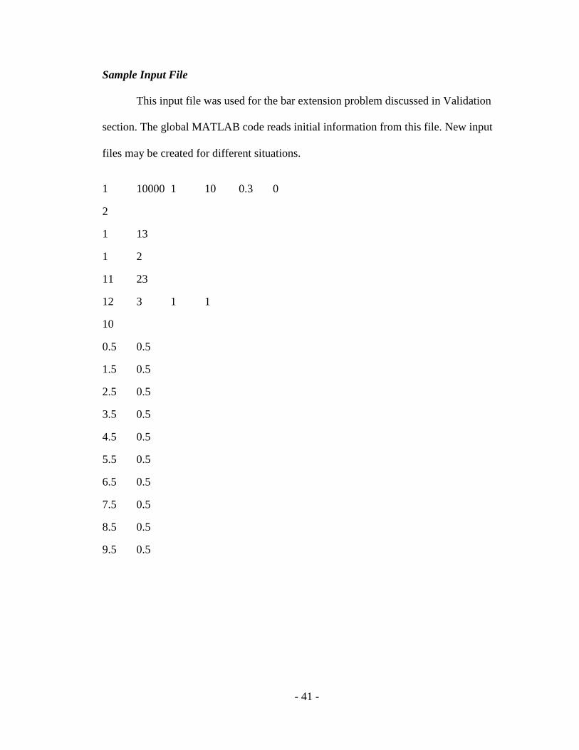
Sample Input File

This input file was used for the bar extension problem discussed in Validation

section. The global MATLAB code reads initial information from this file. New input

files may be created for different situations.

1 10000 1 10 0.3 0

2

1 13

1 2

11 23

12 3 1 1

10

0.5 0.5

1.5 0.5

2.5 0.5

3.5 0.5

4.5 0.5

5.5 0.5

6.5 0.5

7.5 0.5

8.5 0.5

9.5 0.5