an effective model of facets formation
TRANSCRIPT
An Effective Model of Facets Formation
Dima Ioffe1
Technion
April 2015
1Based on joint works with Senya Shlosman, Fabio Toninelli, Yvan Velenikand Vitali Wachtel
Dima Ioffe (Technion ) Microscopic Facets April 2015 1 / 33
Plan of the Talk
A macroscopic variational problem.
Low temperature 3D Ising model, Wulff shapes and (unknown)structure of microscopic facets.
Facets on SOS surfaces with bulk Bernoulli fields.
Fluctuations of level lines.
Dima Ioffe (Technion ) Microscopic Facets April 2015 2 / 33
Macroscopic Variational Problem
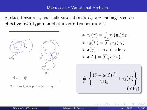
Surface tension τβ and bulk susceptibility Dβ are coming from aneffective SOS-type model at inverse temperature β.
γ7
B = [−1, 1]2
Nested family of loops L = (γ1, . . . , γ7)
γ6
γ2
γ1
γ3 γ5
γ4
τβ(γ) =∫γτβ(ns)ds.
τβ(L) =∑
` τβ(γ`).
a(γ) - area inside γ.
a(L) =∑
` a(γ`).
minL
{(δ − a(L))2
2Dβ
+ τβ(L)
}(VPδ)
Dima Ioffe (Technion ) Microscopic Facets April 2015 3 / 33
Macroscopic Variational Problem: Rescaling
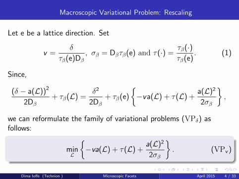
Let e be a lattice direction. Set
v =δ
τβ(e)Dβ
, σβ = Dβτβ(e) and τ(·) =τβ(·)τβ(e)
. (1)
Since,
(δ − a(L))2
2Dβ
+ τβ(L) =δ2
2Dβ
+ τβ(e)
{−va(L) + τ(L) +
a(L)2
2σβ
},
we can reformulate the family of variational problems (VPδ) asfollows:
minL
{−va(L) + τ(L) +
a(L)2
2σβ
}. (VPv )
Dima Ioffe (Technion ) Microscopic Facets April 2015 4 / 33

Geometric Interpretation (Legendre-Fenchel Transform)
τ(a) = min {τ(L) : a(L) = a}
Given v ≥ 0, find minL
{−va + τ(a) +
a2
2σβ
}. (VPv )
τ (a) + a2
2σβ
v∗2
v∗1
v∗3
a−1 a+
1a−2
a+2 a−
3
a
If the graph of a 7→ τ(a) + a2
2σβ
is not convex, then an(infinite) sequence of firstorder transitions with:
Transition slopesv ∗1 , v
∗2 , . . . .
Transition areas a±` .
Dima Ioffe (Technion ) Microscopic Facets April 2015 5 / 33
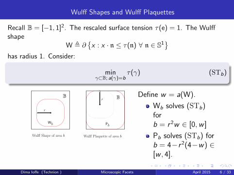
Wulff Shapes and Wulff Plaquettes
Recall B = [−1, 1]2. The rescaled surface tension τ(e) = 1. The Wulffshape
W , ∂{x : x · n ≤ τ(n) ∀ n ∈ S1
}has radius 1. Consider:
minγ⊂B; a(γ)=b
τ(γ) (STb)
Wb Pb
r
rB B
Wulff Plaquette of area bWulff Shape of area b
Define w = a(W).
Wb solves (STb)forb = r 2w ∈ [0,w ]
Pb solves (STb) forb = 4−r 2(4−w) ∈[w , 4].
Dima Ioffe (Technion ) Microscopic Facets April 2015 6 / 33
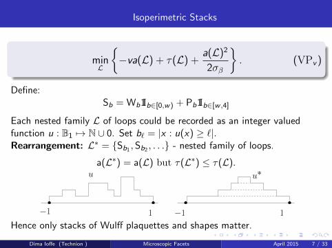
Isoperimetric Stacks
minL
{−va(L) + τ(L) +
a(L)2
2σβ
}. (VPv )
Define:Sb = Wb1Ib∈[0,w) + Pb1Ib∈[w ,4]
Each nested family L of loops could be recorded as an integer valuedfunction u : B1 7→ N ∪ 0. Set b` = |x : u(x) ≥ `|.Rearrangement: L∗ = {Sb1 , Sb2 , . . .} - nested family of loops.
a(L∗) = a(L) but τ(L∗) ≤ τ(L).
−1 −1 11
u u∗
Hence only stacks of Wulff plaquettes and shapes matter.
Dima Ioffe (Technion ) Microscopic Facets April 2015 7 / 33

Regular Isoperimetric Stacks of Type 1 and 2
Recall w = a(W). For any b ∈ (0,w), respectively, b ∈ (w , 4),
d
dbτ (Wb) =
1
r(b)and
d
dbτ (Pb) =
1
r(b).
Which means that optimal stacks of area a could be one of two types:
Stacks L1` (a) of type 1. These contain `− 1 identical Wulff
plaquettes and a Wulff shape, all of the same radius r ∈ [0, 1].
Stacks L2` (a) of type 2. These contain ` identical Wulff plaquettes of
the same radius r ∈ [0, 1].
Set `∗∆= 4
4−w (and assume `∗ 6∈ N). Then, relevant area ranges are:
Range(L1`) =
{[4(`− 1), `w ], if ` < `∗
[`w , 4(`− 1)], if ` > `∗and Range(L2
`) = [`w , 4`]
Dima Ioffe (Technion ) Microscopic Facets April 2015 8 / 33
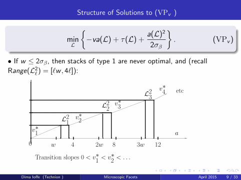
Structure of Solutions to (VPv )
minL
{−va(L) + τ(L) +
a(L)2
2σβ
}. (VPv )
• If w ≤ 2σβ, then stacks of type 1 are never optimal, and (recall
Range(L2` ) = [`w , 4`]):
3w 120
etc
v∗1
Transition slopes 0 < v∗1< v∗
2< . . .
L21
L23
v∗4
L22
v∗3
v∗2
w
a
4 2w 8
Dima Ioffe (Technion ) Microscopic Facets April 2015 9 / 33

Structure of solutions to (VPv )
Recall `∗∆= 4
4−w 6∈ N. For ` < `∗ the area ranges are:
Range(L1`) = [4(`− 1), `w ] and Range(L2
`) = [`w , 4`]
• If w > 2σβ, then then there exists a number 1 ≤ k < `∗(1− σβ
8
)such
that stacks L1` show up for any ` = 1, . . . , k :
0 2w a+2
a−k
Type 2
L22
L21
L11
L12
L2k
a+k
kw
L1k
a−1
a
w a+1
a−2
Dima Ioffe (Technion ) Microscopic Facets April 2015 10 / 33

3D Ising model
∂ΛN
ΛN ⊂ Z3
|ΛN | = N3
The Gibbs State
−H−N =1
2
∑x∼y
σxσy−∑
x∈∂ΛN
σx
P−N,β(σ) ∼ e−βH−N
Low Temperature β � 1 ⇒ m∗(β) > 0.Phase Segregation: Fix m > −m∗ and consider
Pm,−N,β (·) = P−N,β
(·∣∣∑σx = mN3
).
Dima Ioffe (Technion ) Microscopic Facets April 2015 11 / 33

Microscopic 3D Wulff shape
Typical Picture under Pm,−N,β
ΓNVolume of the microscopicWulff droplet
|ΓN | ≈m + m∗
2m∗N3
Theorem (Bodineau, Cerf-Pisztora): As N →∞ the scaled shape1N
ΓN converges to the macroscopic Wulff shape.
Dima Ioffe (Technion ) Microscopic Facets April 2015 12 / 33

3D Surface Tension and Macroscopic Wulff Shape
n +
−
M
+
−
n
Kβ
h
ξβ(n) = − limM→∞
| cos n|M2
logZ±MZ−M
.
ξβ = maxh∈∂Kβ
h · n
Dilated Wulff Shape
Kmβ =
(m + m∗
2m∗|Kβ|
)1/3
Kβ
Dima Ioffe (Technion ) Microscopic Facets April 2015 13 / 33
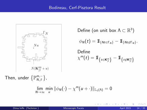
Bodineau, Cerf-Pisztora Result
N (Kmβ + u)
ΓN
Nu
Define (on unit box Λ ⊂ R3)
φN(t) = 1I{Nt∈ΓN} − 1I{Nt 6∈ΓN}.
Defineχm(t) = 1I{t∈Km
β} − 1I{t 6∈Kmβ}
Then, under{Pm,−N,β
},
limN→∞
minu‖φN(·)− χm(u + ·)‖L1(Λ) = 0
Dima Ioffe (Technion ) Microscopic Facets April 2015 14 / 33
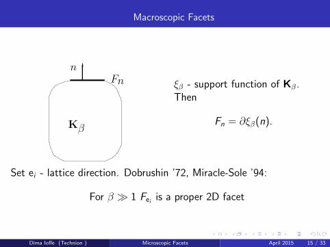
Macroscopic Facets
Kβ
nFn ξβ - support function of Kβ.
Then
Fn = ∂ξβ(n).
Set ei - lattice direction. Dobrushin ’72, Miracle-Sole ’94:
For β � 1 Fei is a proper 2D facet
Dima Ioffe (Technion ) Microscopic Facets April 2015 15 / 33
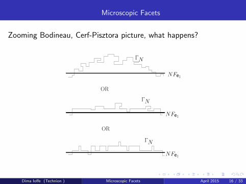
Microscopic Facets
Zooming Bodineau, Cerf-Pisztora picture, what happens?
NFe1
NFe1
NFe1
ΓN
OR
ΓN
OR
ΓN
Dima Ioffe (Technion ) Microscopic Facets April 2015 16 / 33

SOS Model
BN = {−N, . . . , N}2
ΓN
VN
BN = {−N, . . . , N}2
Ak0
k
`N
Bodineau, Schonmann,Shlosman ’05
PN (ΓN = γ) ∼ e−β|γ|
PmN (·) = PN
(·∣∣VN ≥ mN3
)Result: There exists a(β)↘ 0such that
`N = max{k : Ak ≥ a(β)N2
}satisfies A`N−1 ≥ (1− a(β))N2.
Dima Ioffe (Technion ) Microscopic Facets April 2015 17 / 33

Effective Model of Microscopic Facets
ΓN
VN
SN
BN = {−N, . . . , N}2
psβ
pvβ Configuration:(
ΓN , {ξvi }i∈VN,{ξsj}j∈SN
).
Total number of particles:
ΞN =∑i∈VN
ξvi +∑j∈SN
ξsj
|Γ| - area of Γ
Bp(ξ) = pξ(1− p)1−ξ
β large
Probability Distribution:
PN (Γ, ξv , ξs) ∝ e−β|Γ|∏i∈VN
Bpv (ξvi )∏j∈SN
Bps (ξsj ).
Dima Ioffe (Technion ) Microscopic Facets April 2015 18 / 33
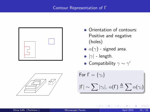
Contour Representation of Γ
Orientation of contours:Positive and negative(holes)
α(γ) - signed area.
|γ| - length.
Compatibility γ ∼ γ′
For Γ = {γi}
|Γ| ∼∑|γi |, α(Γ)
∆=∑
α(γi)
Dima Ioffe (Technion ) Microscopic Facets April 2015 19 / 33

Creation of Facets
ps
pv
α(ΓN )
ΞN - total number of particles
EN (ΞN) =ps + pv
2N3 ∆
= pN3
Consider
PAN (·) = PN
(·∣∣ΞN = pN3 + AN2
)2D Surface Tension: logP
(α(ΓN) = aN2
)≈ −Nτβ(a).
Bulk Fluctuations: ∆ = 2(ps − pv ), EN
(ΞN
∣∣α(ΓN))
= pN3 + ∆α(ΓN).
logPN
(ΞN = pN3 + AN2
∣∣α(ΓN) = aN2)≈ −(AN2 −∆aN2)2
N3R
= −N (δ − a)2
2Dβ, where R = ps(1− ps) + pv (1− pv ),
Dβ = R/(2∆2) and δ = A/∆. Hence mina
{(δ−a)2
2Dβ+ τβ(a)
}.
Dima Ioffe (Technion ) Microscopic Facets April 2015 20 / 33

Surface Tension and Macroscopic Variational Problem
CNx
0 γ
wβ(γ) = e−β|γ|−∑C6∼γ Φβ(γ)
Gβ(Nx) =∑
γ:0→Nx
wβ(γ).
τβ(x) = − limN→∞
1
NlogGβ(Nx).
τβ(γ) =
∫γτβ(ns)ds.
Macroscopic Variational Problem
Recall ∆ = 2(ps − pv ), R = ps(1− ps) + pv (1− pv ) , Dβ = R/(2∆2)and δ = A/∆.
(VP)δ mina
{(δ − a)2
2Dβ+ min
a(L)=aτβ(L)
}.
Dima Ioffe (Technion ) Microscopic Facets April 2015 21 / 33

Reduction to Large Contours
Fix β � 1. Bulk fluctuations simplify analysis of PAN . Recall the contour
representation Γ = {γi}.
Lemma 1 (No intermediate contours). ∀A > 0 there exists ε = ε(A) > 0such that
PAN
(∃γi :
1
εlogN ≤ |γi | ≤ εN
)= o(1).
Lemma 2 (Irrelevance of small contours)
PAN
(∣∣∑α(γi )1I{|γi |≤ε−1 log N}∣∣� N
)= o(1).
Definition: γ is large if |γ| ≥ εN.
Dima Ioffe (Technion ) Microscopic Facets April 2015 22 / 33

Reduced Model of Large Contours
A. Fix A > 0 and forget about intermediate contours 1ε logN ≤ |γ| ≤ εN.
B. Expand with respect to small contours |γ| ≤ 1ε logN.
For Γ = {γi} collection of large contours the effective weight is
PN(Γ) ∝ exp{−β∑ |γi | −∑C6∼Γ Φβ(C)
}.
The family of clusters C depends on N and A. However cluster weightsΦβ(C) remain the same, and they are small: For all β sufficiently large
|Φβ(γ; C)| ≤ ce−β(diam(C)+1)
Reduced Model of Large Contours and Bulk Particles:
PN (Γ, ξv , ξs) = PN(Γ)∏i∈VN
Bpv (ξvi )∏j∈SN
Bps (ξsj )
Dima Ioffe (Technion ) Microscopic Facets April 2015 23 / 33

Limit Shapes Result (I., Shlosman 2015)
Recall: ∆ = 2(ps − pv ), R = ps(1− ps) + pv (1− pv ) , Dβ = R/(2∆2)
and δ = A/∆. (VP)δ mina
{(δ−a)2
D + mina(L)=a τβ(L)}.
a+k∗
A1
A2
A3
Type 2
k∗
Layers
Ak∗
a+1
a−1 a−
2a+2
a−k∗
Set: PAN (·) = PN
(·∣∣ΞN = pN3 + AN2
). Then for any ν > 0 and any
A ≥ 0, the (random) collection of large contours Γ satisfies:
limN→∞ PAN
(minL∗−solutions to (VP)δ
dH(
1N Γ,L∗
)< ν
)= 1
Dima Ioffe (Technion ) Microscopic Facets April 2015 24 / 33
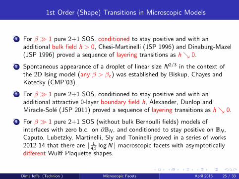
1st Order (Shape) Transitions in Microscopic Models
1 For β � 1 pure 2+1 SOS, conditioned to stay positive and with anadditional bulk field h > 0, Chesi-Martinelli (JSP 1996) and Dinaburg-Mazel(JSP 1996) proved a sequence of layering transitions as h↘ 0.
2 Spontaneous appearance of a droplet of linear size N2/3 in the context ofthe 2D Ising model (any β > βc) was established by Biskup, Chayes andKotecky (CMP’03).
3 For β � 1 pure 2+1 SOS, conditioned to stay positive and with anadditional attractive 0-layer boundary field h, Alexander, Dunlop andMiracle-Sole (JSP 2011) proved a sequence of layering transitions as h↘ 0.
4 For β � 1 pure 2+1 SOS (without bulk Bernoulli fields) models ofinterfaces with zero b.c. on ∂BN , and conditioned to stay positive on BN ,Caputo, Lubetzky, Martinelli, Sly and Toninelli proved in a series of works2012-14 that there are b 1
4β logNc macroscopic facets with asymptoticallydifferent Wulff Plaquette shapes.
Dima Ioffe (Technion ) Microscopic Facets April 2015 25 / 33
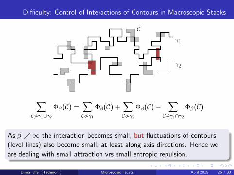
Difficulty: Control of Interactions of Contours in Macroscopic Stacks
C
γ2
γ1
∑C6∼γ1∪γ2
Φβ(C) =∑C6∼γ1
Φβ(C) +∑C6∼γ2
Φβ(C)−∑
C6∼γ1∩γ2
Φβ(C)
As β ↗∞ the interaction becomes small, but fluctuations of contours
(level lines) also become small, at least along axis directions. Hence we
are dealing with small attraction vrs small entropic repulsion.
Dima Ioffe (Technion ) Microscopic Facets April 2015 26 / 33
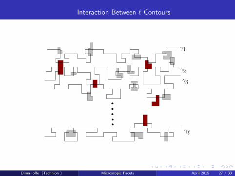
Interaction Between ` Contours
γ1
γ2
γ3
γℓ
Dima Ioffe (Technion ) Microscopic Facets April 2015 27 / 33

A general Result for Ising Polymers
C3
C4
x
y
γ C2
C1 wβ(γ) = e−β|γ|+∑C6∼γ Φβ(γ;C).
Assumption:
|Φβ(γ; C)| ≤ ce−χβ(diam(C)+1).
Theorem (I, Shlosman, Toninelli , JSP 2015)
If χ > 12 , then repulsion wins over attraction for all β sufficiently large, in
the sense that half-space surface tension equals to the full space surface
tension.
Remarks:a. In the case of SOS interfaces χ = 1.
b. The theorem takes care of an interaction between one contour and a
hard wall. Interactions between two, and more generally `, ordered
contours still has to be worked out.Dima Ioffe (Technion ) Microscopic Facets April 2015 28 / 33
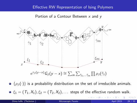
Effective RW Representation of Ising Polymers
Portion of a Contour Between x and y
xy
γ1 γ2γm
ξ1 ξ2xy
ξm
eτβ(y−x)Gβ(y − x) ∼=∑
m
∑γ1,...γm
∏ρβ(γi )
{ρβ(·)} is a probability distribution on the set of irreducible animals.
ξ1 = (T1,X1), ξ2 = (T2,X2), . . . steps of the effective random walk.
Dima Ioffe (Technion ) Microscopic Facets April 2015 29 / 33
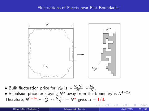
Fluctuations of Facets near Flat Boundaries
ΓN VN
N
Nα
• Bulk fluctuation price for VN is ∼ VNN2
N3 ∼ VNN .
• Repulsion price for staying Nα away from the boundary is N1−2α.
Therefore, N1−2α ∼ VNN ∼ N1+α
N = Nα gives α = 1/3.
Dima Ioffe (Technion ) Microscopic Facets April 2015 30 / 33

Random Walks under Area Tilts
VN
−N N
a
b
X-trajectory of RW
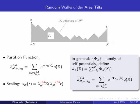
• Partition Function:
Z a,bN,+,λN
=∑
X∈T a,bN,+
e−λNVN p(X)
• Scaling: xN(t) = λ1/3N X(λ
−2/3N t).
In general: {Φλ} - family ofself-potentials, defineΦλ(X) =
∑N−N Φλ(Xi ).
Z a,bN,+,λN
=∑
X∈T a,bN,+
e−ΦλN (X)p(X)
Dima Ioffe (Technion ) Microscopic Facets April 2015 31 / 33
Random Walks under Area Tilts
VN
−N N
a
b
X-trajectory of RW
• Partition Function:
Z a,bN,+,λN
=∑
X∈T a,bN,+
e−λNVN p(X)
• Scaling: xN(t) = λ1/3N X(λ
−2/3N t).
In general: {Φλ} - family ofself-potentials, defineΦλ(X) =
∑N−N Φλ(Xi ).
Z a,bN,+,λN
=∑
X∈T a,bN,+
e−ΦλN (X)p(X)
Dima Ioffe (Technion ) Microscopic Facets April 2015 31 / 33
Random Walks under Area Tilts: Ferrari-Spohn Diffusion
VN
−N N
a
b
X-trajectory of RW
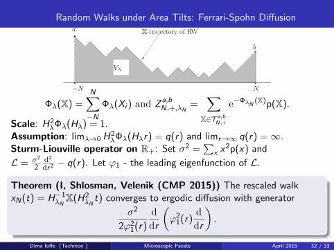
Φλ(X) =N∑−N
Φλ(Xi ) and Z a,bN,+,λN
=∑
X∈T a,bN,+
e−ΦλN (X)p(X).
Scale: H2λΦλ(Hλ) = 1.
Assumption: limλ→0 H2λΦλ(Hλr) = q(r) and limr→∞ q(r) =∞.
Sturm-Liouville operator on R+: Set σ2 =∑
x x2p(x) and
L = σ2
2d2
dr2 − q(r). Let ϕ1 - the leading eigenfunction of L.
Theorem (I, Shlosman, Velenik (CMP 2015)) The rescaled walkxN(t) = H−1
λNX(H2
λNt) converges to ergodic diffusion with generator
σ2
2ϕ21(r)
d
dr
(ϕ2
1(r)d
dr
).
Dima Ioffe (Technion ) Microscopic Facets April 2015 32 / 33
` Ordered Random Walks under Area Tilts
b2
a2
a1
b1X2
X1
X`
−N N
a`
b`
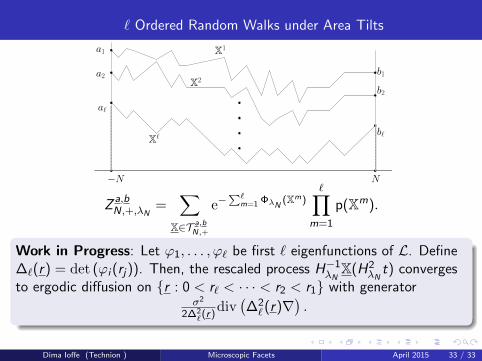
Za,bN,+,λN
=∑
X∈T a,bN,+
e−∑`
m=1 ΦλN (Xm)∏m=1
p(Xm).
Work in Progress: Let ϕ1, . . . , ϕ` be first ` eigenfunctions of L. Define∆`(r) = det (ϕi (rj)). Then, the rescaled process H−1
λNX(H2
λNt) converges
to ergodic diffusion on {r : 0 < r` < · · · < r2 < r1} with generatorσ2
2∆2`(r)
div(∆2` (r)∇
).
Dima Ioffe (Technion ) Microscopic Facets April 2015 33 / 33