an efficient adaptive mesh redistribution method for a non-linear dirac equation

Journal of Computational Physics 222 (2007) 176–193

www.elsevier.com/locate/jcp

An efficient adaptive mesh redistribution method for anon-linear Dirac equation

Han Wang, Huazhong Tang *

LMAM, School of Mathematical Sciences, Peking University, 5# YiHe Yuan Lu, Haidian District, Beijing 100871, PR China

Received 7 March 2006; received in revised form 9 July 2006; accepted 20 July 2006Available online 30 August 2006

Abstract

This paper presents an efficient adaptive mesh redistribution method to solve a non-linear Dirac (NLD) equation. Ouralgorithm is formed by three parts: the NLD evolution, the iterative mesh redistribution of the coarse mesh and the localuniform refinement of the final coarse mesh. At each time level, the equidistribution principle is first employed to iterativelyredistribute coarse mesh points, and the scalar monitor function is subsequently interpolated on the coarse mesh in orderto do one new iteration and improve the grid adaptivity. After an adaptive coarse mesh is generated ideally and finally,each coarse mesh interval is equally divided into some fine cells to give an adaptive fine mesh of the physical domain,and then the solution vector is remapped on the resulting new fine mesh by an affine method. The NLD equation is finallysolved by using a high resolution shock-capturing method on the (fixed) non-uniform fine mesh.

Extensive numerical experiments demonstrate that the proposed adaptive mesh method gives the third-order rate ofconvergence, and yields an efficient and fast NLD solver that tracks and resolves both small, local and large solution gra-dients automatically.� 2006 Elsevier Inc. All rights reserved.

Keywords: Adaptive mesh redistribution; The Dirac equation; Local uniform refinement; Solitary wave; High resolution scheme

1. Introduction

Ever since its invention in 1929 the Dirac equation has played a fundamental role in various areas ofmodern physics and mathematics, and is important for the description of interacting particles and fields.In past three decades, several authors have committed themselves to analytically investigating the non-lin-ear Dirac (NLD) model, see [4,6–8,31,32] and references therein. Some reliable, higher-order accuratenumerical methods have also been constructed to solve the NLD model. They are Crank–Nicholson typeschemes [3,5], split-step spectral schemes [17], Legendre rational spectral methods [46], multi-symplecticRunge–Kutta methods [22], and Runge–Kutta discontinuous Galerkin (RKDG) methods [35], etc. Theinteraction dynamics for the one-humped Dirac solitary waves were investigated in [5] by using a

0021-9991/$ - see front matter � 2006 Elsevier Inc. All rights reserved.

doi:10.1016/j.jcp.2006.07.011

* Corresponding author. Tel.: +86 10 62757018; fax: +86 10 62751801.E-mail addresses: [email protected] (H. Wang), [email protected] (H. Tang).

mailto:[email protected]

mailto:[email protected]

H. Wang, H. Tang / Journal of Computational Physics 222 (2007) 176–193 177

second-order accurate difference scheme. The weakly inelastic interaction in ternary collisions is firstreported in [35]. In [36,37], the second author and his co-worker further observed the strong inelasticinteraction in ternary collisions, and investigated interaction dynamics of two-humped Dirac solitarywaves with or without an initial phase shift.

In studying the interaction dynamics of the Dirac solitary waves, the physical solutions are usually verysingular in fairly localized regions. To resolve these large solution variations, numerical simulations requireextremely fine meshes on those small localized portions of the physical domain. They will become very expen-sive if a uniform fine mesh is used. Otherwise, the numerical wave will incorrectly propagate due to under-res-olution of the waves. Hence it is very necessary to develop an effective adaptive grid method for the NLDmodel. Successful implementation of an adaptive strategy can increase accuracy of numerical approximationand also decrease computational costs.

Adaptive moving mesh methods have important applications in solving partial differential equations(PDEs). Up to now, there have been important progresses, including the variational approach of Winslow[47], Brackbill and Saltzman [11,12], Dvinsky [18] and Li et al. [25,26]; moving finite element methods of Millerand Miller [29], Davis and Flaherty [16], and Beckett et al. [10]; and moving mesh PDEs of Cao et al. [13,14],Li and Petzold [27], Ceniceros and Hou [15] and Ren and Wang [33] as well as [45], etc. Harten and Hyman[21] began the earliest study of the self-adaptive moving mesh methods to improve resolution of discontinuoussolutions of hyperbolic equations. After their work, many other moving mesh methods in this direction havebeen proposed based on combining the variational grid methods with high resolution shock capturing meth-ods. They include works of Azarenok et al. [9], Fazio and LeVeque [19], Liu et al. [28], Saleri and Steinberg[34], Stockie et al. [39], Tang et al. [40–42], Zegeling et al. [48,49] and Zhang [50]. We refer the readers to arecent paper [43] for a detailed review. However, to our knowledge, there is no any research work on adaptivemoving mesh methods for the NLD model in the literatures.

The aim of this paper is to present an efficient adaptive mesh redistribution method for the NLD modelbased on the adaptive moving mesh method for hyperbolic conservation laws, proposed by Tang and Tangin [41]. The present adaptive mesh algorithm will include three parts: the NLD evolution, an iterative redis-tribution of the coarse mesh, and the local uniform refinement of the final coarse mesh. The NLD evolutionmay be any appropriate high resolution finite volume scheme. While the coarse mesh redistribution is an iter-ative procedure. In each iteration, the coarse mesh points are first iteratively redistributed by the equidistri-bution principle, and then the scalar monitor function is updated on the resulting new coarse mesh toimprove the grid adaptivity. After the final adaptive coarse mesh is generated ideally, each coarse mesh ele-ment is equally divided into some fine cells to give an adaptive fine mesh of the physical domain, and thenthe solution vector is remapped from the initial fine mesh to the new fine mesh by the affine method. Thesecombinations will yield a powerful and fast NLD solver that tracks and resolves both small, local and largesolution gradients automatically. It is worth mentioning that our proposed method may be considered as acombination of the r-refinement method and the h-refinement method and shares the same idea of the two-level mesh movement technique of Huang et al. [23,24] and Fiedler and Trapp [20] as well as the hr-refinementmethod in the literatures, see e.g. [1,2,30].

This paper is organized as follows. In Section 2 we briefly review the NLD model as well as its two exactsolitary wave solutions. In Section 3, we begin to present an adaptive moving mesh method for the NLD equa-tion. Section 4 conducts some numerical experiments to validate the accuracy and capability of the proposedapproach. The numerical examples include binary, ternary, and quadruple collisions of the Dirac solitarywaves. Emphatically, quadruple collisions of the Dirac solitary waves are investigated for the first time. Weconclude the paper with a few remarks in Section 5.

2. Preliminaries

Consider a classical spinorial model with scalar self-interaction, described by the non-linear LagrangianL ¼ iwclolw� mwwþ kðwwÞ2 from which we may derive the non-linear Dirac equation (NLD)

iclolw� mwþ 2kðwwÞw ¼ 0; ð1Þ

178 H. Wang, H. Tang / Journal of Computational Physics 222 (2007) 176–193

where i ¼ffiffiffiffiffiffiffi�1p

;w is the complex conjugate of w, k and m are two real constants, and the matrices cl are de-fined by

c0 ¼I 0

0 �I

� �; ck ¼

0 rk

�rk 0

� �;

here rk with k = 1,2,3, denote the Pauli matrices. The non-linear self-coupling term ðwwÞ2 in the Lagrang-ian allows the existence of finite energy, localized solitary waves, or extended particle-like solutions, see e.g.[38].

We restrict our attention to the (1 + 1)-dimensional NLD model (1), and use the notations qE(x, t), qP(x, t)and qQ(x, t) to denote the energy density, the linear momentum density and the charge density, which aredefined by

qEðx; tÞ ¼ Imðw1oxw2 þ w2oxw1Þ þ mðjw1j2 � jw2j

2Þ � kðjw1j2 � jw2j

2Þ2; ð2ÞqP ðx; tÞ ¼ Imðw1oxw1 þ w2oxw2Þ; ð3ÞqQðx; tÞ ¼ jw1j

2 þ jw2j2; ð4Þ

where w1 and w2 are two components of the spinor w(x, t). Then we have the (total) energy E, the linearmomentum P and the charge Q as follows

EðtÞ ¼Z

R

qEðx; tÞdx; P ðtÞ ¼Z

R

qP ðx; tÞdx; QðtÞ ¼Z

R

qQðx; tÞdx; ð5Þ

which are conservative, if limjxj!+1jwj = 0 and limjxj!+1joxwj < +1 hold uniformly for t P 0.The (1 + 1)-dimensional NLD equation (1) has two exact solutions, which will be used in our numerical

experiments. The first is the standing wave solution at x = x0 defined by

wswðx� x0; tÞ �wsw

1 ðx� x0; tÞwsw

2 ðx� x0; tÞ

� �¼

Aðx� x0ÞiBðx� x0Þ

� �e�iKt ð6Þ

with

AðxÞ ¼

ffiffiffiffiffiffiffiffiffiffiffiffiffiffiffiffiffiffiffiffiffiffiffiffiffiffiffiffiffiffiffiffiffiffiffiffiffiffiffi1k ðm2 � K2Þðmþ KÞ

qcosh x

ffiffiffiffiffiffiffiffiffiffiffiffiffiffiffiffiffiffiffiffiffiðm2 � K2Þ

q� �mþ K cosh 2x


q� � ; ð7Þ

BðxÞ ¼

ffiffiffiffiffiffiffiffiffiffiffiffiffiffiffiffiffiffiffiffiffiffiffiffiffiffiffiffiffiffiffiffiffiffiffiffiffiffiffi1k ðm2 � K2Þðm� KÞ

qsinh x


q� �mþ K cosh 2x


q� � : ð8Þ

Here 0 < K 6 m.The second exact solution of the Dirac model (1) is the single solitary wave solution placed initially at x0

with a velocity v:

wssðx� x0; tÞ ¼ ðwss1 ðx� x0; tÞ;wss

2 ðx� x0; tÞÞT ; ð9Þ
where
wss1 ðx� x0; tÞ ¼

ffiffiffiffiffiffiffiffiffiffifficþ 1

2

rwsw

1 ð~x;~tÞ þ signðvÞffiffiffiffiffiffiffiffiffiffiffic� 1

2

rwsw

2 ð~x;~tÞ; ð10Þ

wss2 ðx� x0; tÞ ¼

ffiffiffiffiffiffiffiffiffiffifficþ 1

2

rwsw

2 ð~x;~tÞ þ signðvÞffiffiffiffiffiffiffiffiffiffiffic� 1

2

rwsw

1 ð~x;~tÞ; ð11Þ

here c ¼ 1=ffiffiffiffiffiffiffiffiffiffiffiffiffi1� v2p

, ~x ¼ cðx� x0 � vtÞ, ~t ¼ cðt � vðx� x0ÞÞ, wsw1 and wsw

2 are defined in (6) and sign(x) is thesign function, which returns 1 if x > 0, 0 if x = 0 and �1 if x < 0. The solution wss(x � x0, t) represents a sol-

0 2 4 6

0.2

0.23094

0.280056

0.333333

0.458831

x

Qv = 0.9v = 0.8v = 0.7v = 0.5v = 0

0 2 4 6

5

5.7735

7.0014

8.33333

11.4708

x

Qv = 0.9v = 0.8v = 0.7v = 0.5v = 0

-2-4-6 -2-4-6

Fig. 1. Dependence of qQ on K and v. Left: K = 0.9; right: K = 0.1.


itary wave travelling from left to right if v > 0, or travelling from right to left if v < 0, and the standing wavewsw(x � x0, t) is actually a solitary wave at rest placed at x0 or identical to wss(x � x0, t) with v = 0.

The profile of the solution (6) or (9) is strongly dependent on the parameter K:

� it is a two-humped solitary wave with two peaks whose locations are determined by

coshð2ffiffiffiffiffiffiffiffiffiffiffiffiffiffiffiffiffim2 � K2p

~xÞ ¼ m2�K2

mK if 0 < K < m2;

� it becomes a one-humped solitary wave with one peak located at ~x ¼ 0 if m26 K < m; and

� wss(x � x0, t) ” 0 if K = m.

Moreover, amplitude of the solitary waves also depends strongly on the velocity v: qssQðx� x0; tÞ ¼ cqsw

Q ð~x;~tÞ.Fig. 1 shows that dependence, which will give different interaction dynamics. We also refer the readers to [35–37] for more detailed investigations. It is worth noting that eihwss(x � x0, t) is still a solitary wave solution ofthe (1 + 1)-dimensional Dirac model (1), if h is a constant.

For actual numerical computations, we decompose the complex function w1(x, t) and w2(x, t) into its realand imaginary parts by writing

wiðx; tÞ ¼ wri ðx; tÞ þ iws

i ðx; tÞ; i ¼ 1; 2

and then rewrite the (1 + 1)-dimensional NLD model (1) in a conservative form of real variables

ou

otþ of ðuÞ

ox¼ sðuÞ; ð12Þ

where u ¼ ðwr1;w

s1;w

r2;w

s2Þ

T; sðuÞ ¼ gðx; tÞðws

1;�wr1;�ws

2;wr2Þ

T , and

f ðuÞ ¼ Au �

0 0 1 0

0 0 0 1

1 0 0 0

0 1 0 0

0BBB@1CCCA

wr1

ws1

wr2

ws2

0BBB@1CCCA;

here g(x, t) :¼ m + 2k(jw2j2 � jw1j2), and jwij2 ¼ ðwr

i Þ2 þ ðws

i Þ2; i ¼ 1; 2.

3. An adaptive mesh method

This section presents an adaptive moving mesh finite volume approach for the (1 + 1)-dimensional NLDmodel, which is an extension of the method introduced by Tang and Tang [41]. To increase efficiency, we onlyapply the iterative grid redistribution technique to the coarse mesh, and then refine uniformly each final coarse


mesh interval. That will yield a powerful and fast NLD solver that tracks and resolves both small, local andlarge solution gradients automatically.

3.1. Coarse mesh redistribution

Let x and n denote the physical and logical coordinates, respectively. A one-to-one coordinate transforma-tion from logical domain Xl = [0,1] to the physical domain Xp = [a,b] is denoted by

x ¼ xðnÞ; n 2 Xl:

Its inversion is denoted by

n ¼ nðxÞ; x 2 Xp:

If giving a uniform partition of the logical domain Xl such as 0 = n0 < n1 <� � �< nN = 1, (nj = j/N,j = 0,1,2, . . . ,N), then we usually use the coordinate transformation x = x(n) to give an ‘‘adaptive’’ mesh ofthe physical domain Xp: a = x0 < x1 <� � �< xN = b, where xj = x(nj), j = 0,1,2, . . . ,N. To derive the coordinatetransformation, we employ the well-known equidistribution principle, and then have

ðxxnÞn ¼ 0; n 2 Xl; ð13Þ

subject to boundary conditions x(0) = a and x(1) = b. Here, x is a positive weight function, i.e. the so-calledmonitor function. A widely used monitor function is defined by

x ¼ffiffiffiffiffiffiffiffiffiffiffiffiffiffiffiffiffiffiffiffiffiffiffiffiffiffiffiffiffiffiffiffiffiffiffi1þ ajuj2 þ bjuxj2

q: ð14Þ

Solving (13) will end up with a desired mesh map x = x(n). In this work, we use an iteration method, such asGauss–Siedel iteration method, to solve the mesh redistribution equation (13), i.e.

x x½m�jþ1

2

� �x½m�jþ1 � x½mþ1�

j

� �� x x½m�

j�12

� �x½mþ1�

j � x½mþ1�j�1

� �¼ 0 ð15Þ

for j = 1,2, . . .N � 1, where m = 0,1, . . .For most implementations of the mesh redistribution, the iteration number m in (15) is usually controlled

under a tolerance denoted by l, in order to save CPU time. However, if the wave propagation speed becomeslarge, then the equidistribution principle cannot be perfectly preserved in numerical computations, unless wetake a very large value of l. To overcome the above disadvantage, we employ a local uniform refinement tech-nique, that is to say, we only redistribute coarse mesh points by (15) iteratively, and then divide the final coarsecell (i.e. m = l) into some locally equal fine cells. Assume N = N0N1, where N0 and N1 are two positive integers,and use {xj, j = 0,N0,2N0, . . . ,N1N0} to denote the coarse mesh. Then applying the above iterative mesh redis-tribution, e.g. (15), to the coarse mesh {xj, j = 0,N0,2N0, . . . ,N1N0} gives

x x½m�jþN0

2

� �x½m�jþN0

� x½mþ1�j

� �� x x½m�

j�N02

� �x½mþ1�

j � x½mþ1�j�N0

� �¼ 0 ð16Þ

for j = N0,2N0, . . . , (N1 � 1)N0, where m = 0,1, . . . ,l � 1.

3.2. Interpolation of the monitor function on the coarse mesh

After each iteration of the mesh redistribution, the moving mesh finite volume approach of Tang and Tang

[41] should remap the solution u on the new mesh x½mþ1�j

n oN

j¼0by a high resolution conservative interpolation,

according to the known data x½m�j

n oN

j¼0as well as u

½m�jþ1

2

n oN�1

j¼0, and then calculate x½mþ1�

jþ12

for next iteration. It is

proved that such remapping phase is successful and robust in capturing strong discontinuities (shock waves,etc.) in fluid flows.

However, since the iterative grid redistribution is solely implemented on the coarse mesh in the presentalgorithm, the remapping phase may be operated on the same coarse mesh. To further save the computational


cost, we will directly remap the scalar monitor function x on the coarse mesh fx½mþ1�j ; j ¼ 0;N 0; 2N 0; . . . ;N 1N 0g

instead of the solution vector u = (u1,u2,u3,u4)T.

Assume that we have solved (16) to yield fx½mþ1�j ; j ¼ 0;N 0; 2N 0; . . . ;N 1N 0g. Since it is not important whether

the function x is conservative, we may consider x½m�jþN0

2

as an approximation of x x½m�jþN0

2

� �and remap x by a

simple linear interpolation such as

x½m�jþN0

2

¼ x½0�kþN0

2

þx½0�

kþN02

� x½0�k�N0

2

x½0�kþN0

2

� x½0�k�N0

2

x½m�jþN0

2

� x½0�kþN0

2

� �; ð17Þ� �

if x½m�jþN0

2

2 x½0�k�N0

2

; x½0�kþN0

2

, where m P 1. It is worth noting that we always interpolate the monitor function x½m�jþN0

2

by using the ‘‘initial’’ data x½0�jþN0

2

.

Remark 3.1. The advantage of the interpolation (17) is that at each time level we only need to compute the‘‘initial’’ first-order divided difference, see (17), during the iterative redistribution of the coarse mesh.

Remark 3.2. The initial value of the monitor function x½0�jþN0

2

is computed by using a discrete form of (14) withthe volume average of u

½0�jþ1

2

over the fine cell, i.e.

u½0�jþN0

2

¼ 1

Dx½0�jþN0

2

XN0

l¼1

Dx½0�jþl

2

u½0�jþl

2

: ð18Þ

Remark 3.3. We may also consider xjþN0

2as cell averages of the monitor function x over the cell ½xj; xjþN0

�, andthen employ the interpolation approach as introduced by Tang et al. [41] to remap the monitor function x onthe new mesh fx½mþ1�

j ; j ¼ 0;N 0; 2N 0; . . . ; ðN 1 � 1ÞN 0g as follows

Dx½mþ1�jþN0

2

x½mþ1�jþN0

2

¼ Dx½m�jþN0

2

x½m�jþN0

2

� ðccxÞ½m�jþN0� ðccxÞ½m�j

� �ð19Þ

for j = 0,N0,2N0, . . . , (N1 � 1)N0, where DxjþN0

2¼ xjþN0

� xj, and

ðccxÞj ¼ cj

2ðxj;R þ xj;LÞ �

jcjj2ðxj;R � xj;LÞ; ð20Þ

here cj ¼ x½m�j � x½mþ1�j , and

xj;L ¼ xj�N0

2þ 1

2S

j�N02; xj;R ¼ x

jþN02� 1

2S

jþN02:

The slope limiter Sj�12

is an approximation of the derivative oxon at n ¼ nj�1

2. In our computations, we employ the

van Leer limiter [44]

SjþN0

2¼�

sign DxjþN0

2

� �þ sign Dx

j�N02

� �� jDxjþN0

2Dx

j�N02j

jDxjþN0

2j þ jDx

j�N02j þ e

;

where DxjþN0

2¼ x

jþ3N02

� xjþN0

2, and 0 < e� 1 is used to avoid that the denominator becomes zero.

3.3. Local uniform refinement and remapping the solution

Assuming that the final adaptive coarse mesh fx½l�j ; j ¼ 0;N 0; 2N 0; . . . ; ðN 1 � 1ÞN 0g has been generated, we

divide equally each coarse mesh interval or element ½x½l�j ; x½l�jþN0�; j ¼ 0;N 0; . . . ; ðN 1 � 1ÞN 0, into N0 fine mesh

cells and yield the fine grid points fx½l�i ; i ¼ j� N 0; j� N 0 þ 1; . . . ; j� 1g; j ¼ N 0; 2N 0; . . . ;N 1N 0. As a result,

we get an adaptive fine mesh of the physical domain Xp: fx½l�j gNj¼0. Fig. 2 displays the procedure of the fine mesh

j

j

j+3

j+3

j-3

j-3

Fig. 2. The fine mesh redistribution with a local uniform refinement. N0 = 3.


redistribution with a local uniform refinement, where N0 = 3, symbol ‘‘s’’ denotes the coarse mesh pointwhich is first redistributed by solving mesh redistribution equation iteratively, and symbol ‘‘·’’ is the meshpoint obtained by a local uniform refinement. It is worth mentioning that our method may be consideredas a combination of the r-refinement method and the h-refinement method and shares the same idea of thetwo-level mesh movement technique of Huang et al. [23,24] and Fiedler and Trapp [20] as well as the hr-refine-ment method in the literatures, see e.g. [1,2,30].

Now we need to remap the solution vector u from the old fine mesh fx½0�j gNj¼0 :¼ T ½0� to the new fine mesh

T[l]. Each cell of T[l] corresponds uniquely to a cell of T[0] by xjðsÞ ¼ x½0�j þ sdx½0�j where dx½0�j :¼ x½l�j � x½0�j ,

s 2 [0,1]. There is an affine map denoted by x = x(n,s) between the two cells ½x½0�j ; x½0�jþ1� and ½x½l�j ; x

½l�jþ1�. The

profile of u on Xp will not move, although the nodes of the mesh have been moved to new locations. Henceu, as the function of x at a fixed time t, is independent on the parameter s. That is

ou

os¼ 0; s 2 ½0; 1�: ð21Þ

During the movement of the mesh, u may be expressed as

u ¼ uðxÞ ¼ uðx; sÞ ¼ uðxðn; sÞ; sÞ:
Integrating (21) over [xj(s), xj+1(s)] gives
d

ds

Z xjþ1ðsÞ

xjðsÞudx� ðxsuÞjþ1 þ ðxsuÞj ¼ 0; s 2 ½0; 1�: ð22Þ

This equation will be solved by a high-resolution shock-capturing scheme combined with a second-orderRunge–Kutta time discretization, which is described in the subsequent section.

In Section 4, we will validate that the fine mesh redistribution with the local uniform refinement is morepowerful and faster than the original adaptive mesh method introduced in [41].

3.4. The NLD solver on a fixed mesh

Assume that we have obtained the new mesh T ½l� :¼ fx½l�j gNj¼0. In the following, we solve (12) on the fixed

non-uniform mesh T[l], that is to say, x½l�j is independent on t 2 [tn, tn + Dtn).

Integrating (12) over the control volume ½x½l�j ; x½l�jþ1� leads to the following semi-discrete finite volume method

x½l�jþ1 � x½l�j

� � dujþ12ðtÞ

dt¼ �ðf jþ1 � f jÞ þ

Z x½l�jþ1

x½l�j

sðuÞdx; ð23Þ


where f j is some appropriate numerical flux satisfying

f j ¼ f ðuj;L; uj;RÞ; f ðu; uÞ ¼ f ðuÞ: ð24Þ
An example of the numerical flux is the Lax–Friedrichs type flux:
f ðv;wÞ ¼ 1

2½f ðwÞ þ f ðvÞ � rðw� vÞ�; ð25Þ

where r P maxu k ofou

�� . In (24), uj,L and uj,R are defined by

uj;L ¼ uj�12þ Sj�1

2x½l�j �

x½l�j�1 þ x½l�j

2

!; ð26Þ

uj;R ¼ ujþ12þ Sjþ1

2x½l�j �

x½l�j þ x½l�jþ1

2

!: ð27Þ

The slope limiters Sjþ12¼ S1

jþ12; S2

jþ12; S3

jþ12; S4

jþ12

� �Tin (26) and (27) are defined by

Sijþ1

2¼ sign Si;þ

jþ12

� �þ sign Si;�

jþ12

� �� Si;þjþ1

2

Si;�jþ1

2

�� Si;þ

jþ12

�� þ Si;�jþ1

2

�� þ e; i ¼ 1; 2; 3; 4;

where 0 < e� 1 is used to avoid that the denominator becomes zero. Here,

Sþjþ12¼

ujþ32� ujþ1

2

x½l�jþ3

2

� x½l�jþ1

2

; S�jþ12¼

ujþ12� uj�1

2

x½l�jþ1

2

� x½l�j�1

2

:

Since
Z x½l�jþ1
x½l�j

sðuÞdx Dx½l�jþ1

2

s ujþ12

� �: ð28Þ

Thus Eq. (23) can be further approximated as follows

d

dtujþ1

2¼ � 1

Dx½l�jþ1

2

f jþ1 � f j

� �þ s�

ujþ12

�: ð29Þ

The semi-discrete scheme (29) gives a system of ordinary differential equations with respect to the unknownvector u, which may be written in a matrix-operator form

du

dt¼ Lðt; uÞ: ð30Þ

We apply an explicit second-order accurate Runge–Kutta method to discretization of the time derivative in(30) or (29). The Runge–Kutta method we consider is

K1 ¼ DtnLðtn; unÞ;

K2 ¼ DtnLðtn þ 12Dtn; u

n þ 12K1Þ;

unþ1 ¼ un þ K2:

8><>: ð31Þ

The semi-discrete MUSCL-type finite volume method (29) and (31), which is of second order accuracy insmooth regions in the sense of the truncation error, will be applied to (22) and the NLD Eq. (1) in our com-putations. When the above method is applied to (22), it is just marched forward in s by one unit step size, i.e.Ds = 1. Note that (xs)j and xj s ¼ 1

2

are specified as

ðxsÞj ¼ x½l�j � x½0�j ; xj s ¼ 1

2

� �¼ 1

2x½l�j þ x½0�j

� �:


The time step-size for the NLD equation (1) is determined by the CFL condition

Dtn 6 cflmin Dx½l�

jþ12

n or

; max kof

ou

� �� 6 r; ð32Þ

where cfl denotes the CFL number.

3.5. Solution procedure

Our solution procedure is based on three parts: the NLD evolution, the iterative mesh redistribution of thecoarse mesh, and the local uniform refinement of the final coarse mesh. That procedure can be illustrated bythe following flowchart.

Algorithm 1

Step 1. Compute the cell average of the initial data u0jþ1

2

n oand give a uniform mesh

�x0

j

N

j¼0at t = 0.

Step 2. For j = 0,N0,2N0, . . . ,N1N0, define x½0�j :¼ xnj , x½0�

jþN02

:¼ xnjþN0

2

, where n P 0. For m = 0,1, . . ., dothe following:

(a) Move the coarse meshn

x½m�j

oton

x½mþ1�j

oby solving (16).

(b) Compute

�x½mþ1�

jþN02

�by using (17) or (19).

(c) Repeat the updating procedure (a) and (b) for a fixed number of iterations l or until

ix[m+1] � x[m]i 6 e where iÆi is the discrete norm on the coarse mesh.

Step 3. Divide equally the coarse mesh intervalhx½l�j�N0

; x½l�j

iinto N0 fine cells, let xnþ1

j :¼ x½l�j , and remap

the solution u from the old fine mesh�

xnj

N

j¼0to the new fine mesh

�xnþ1

j

N

j¼0by the affine method (22).

Step 4. Evolve the Dirac equation using the high-resolution finite volume method on the fine mesh�xnþ1

j

N

j¼0.

Step 5. Iftn+1 < T, then go to Step 2. Otherwise, output the result and stop.

4. Numerical experiments

This section will conduct numerical experiments to demonstrate the performance and efficiency of the adap-tive mesh method proposed in the last section. All computations work in dimensionless units, or equivalently,take m = 1 and k ¼ 1

2, and adopt the non-reflecting boundary conditions at artificial boundaries. The CFL

number cfl and parameters N1 and l are taken as 0.5, 100 and 10, respectively, unless stated otherwise.Our codes are run on an IBM laptop (Pentium-M, 1.8 GHz) under the Linux environment. We define the griddensity by 1/Dxj+1/2 to depict the grid quality.

For convenience, we will use the notations Algorithm 0 and Algorithm 1 to denote two different adaptivemoving mesh methods, which are

� Algorithm 0 – the adaptive moving mesh method of Tang and Tang [41], in which the fine mesh is iteratively

redistributed and the solution vector is remapped on the resulting new fine meshn

x½mþ1�j

oN

j¼1from the old

meshn

x½m�j

oN

j¼1in each iteration.


� Algorithm 1 – the present method with the local uniform refinement, in which the coarse mesh is just redis-tributed iteratively and the monitor function x is remapped on the resulting new coarse meshn

x½mþ1�j ; j ¼ 0;N 0; . . . ;N 1N 0

ofrom the old mesh fx½m�j ; j ¼ 0;N 0; . . . ;N 1N 0g in each iteration. We yield the

adaptive fine meshn

x½0�j

oN

j¼1of the physical domain Xp by the local uniform refinement.

Example 4.1 (Single travelling solitary wave). The first example is to simulate travel of a two-humped Diracsolitary wave. Since the exact single soliton solution (9) to the (1 + 1)-dimensional NLD equation (1) isknown, we can compare our numerical solutions with the exact solution, and then evaluate the efficiency ofour proposed algorithm. Here we take the monitor function (14) with a = 10 and b = 20 and K = 0.1, x0 = �5,v = 0.1. The physical domain Xp is considered as [�25,25].

Tables 1 and 2 give numerical errors at t = 100 and convergence rates for Algorithm 0 and Algorithm 1.Those estimated errors are defined by

TableExamp

N

l1-erro

l2-erro

l1-erro

CPU t

l1-error :¼ 1

4

X4

i¼1

Xj

ðuei Þjþ1

2� ðuc

i Þjþ12

�� ðxjþ1 � xjÞ;

l2-error :¼

ffiffiffiffiffiffiffiffiffiffiffiffiffiffiffiffiffiffiffiffiffiffiffiffiffiffiffiffiffiffiffiffiffiffiffiffiffiffiffiffiffiffiffiffiffiffiffiffiffiffiffiffiffiffiffiffiffiffiffiffiffiffiffiffiffiffiffiffiffiffiffiffiffiffiX4

i¼1

Xj

ðuei Þjþ1

2� ðuc

i Þjþ12

�� 2ðxjþ1 � xjÞ

vuut ;

l1-error :¼ maxi;j

ðuei Þjþ1

2� ðuc

i Þjþ12

�� n o;

where ðue1; u

e2; u

e3; u

e4Þjþ1

2denote the cell averages of the exact solution ue over [xj,xj+1], while ðuc

1; uc2; u

c3; u

c4Þ

T is the

computed solution. We see that Algorithm 1 is more accurate and less time-consuming than Algorithm 0. Con-cretely, the accuracy of Algorithm 0 decreases as N increases, while Algorithm 1 gives a uniform third-orderrate of convergence independent on N. The results show that Algorithm 1 may give a super-convergent solu-tion and is not insensitive to smoothness and size of the mesh. By contraries, Algorithm 0 is strongly sensitiveto smoothness and size of the mesh. Moreover, Algorithm 1 may save about 86% cost in the present compu-tations, compared to Algorithm 0.

To further validate the performance and efficiency of Algorithm 1, we present the mesh densities (solid line)and the charge densities (black dot) in Figs. 3 and 4, obtained by using Algorithm 0 and Algorithm 1, wherescale of the left axis is for the charge density and the right one is for the mesh density. From the left figure ofFig. 3, we see that the grid points at t = 100 redistributed by Algorithm 0 mainly cluster in the vicinity of theleft peak of the Dirac solitary wave when the iterative tolerance l equals to 10. Thus the mesh is not equallydistributed. If we increase l up to 30, the redistribution of the mesh points has been improved in the numericalcomputations, see the right figure of Fig. 3, but we have sacrificed quite a bit CPU time. The result given in theleft figure of Fig. 4 shows that Algorithm 1 implements easily and fast the equidistribution principle, and themesh density of Algorithm 1 preserves symmetry just as two peaks of the Dirac solitary wave are symmetric. Sothe quality of the adaptive mesh generated by Algorithm 1 is very perfect. The right plot of Fig. 4 gives the time

1le 4.1. Numerical errors and convergence rates of Algorithm 0 at t = 100

100 200 400 800 1600 3200

r order 3.786 5.178e�1 7.565e�2 1.279e�2 3.465e�3 1.274e�03– 2.87 2.78 2.56 1.88 1.44

r order 2.992 4.089e�1 5.909e�2 9.840e�3 2.573e�3 9.477e�04– 2.87 2.79 2.59 1.94 1.44

r order 1.004 1.309e�1 1.949e�2 3.670e�3 1.077e�3 3.979e�04– 2.94 2.75 2.41 1.77 1.44

ime (s) 6.11 21.46 83.76 335.69 1325.50 4940.00

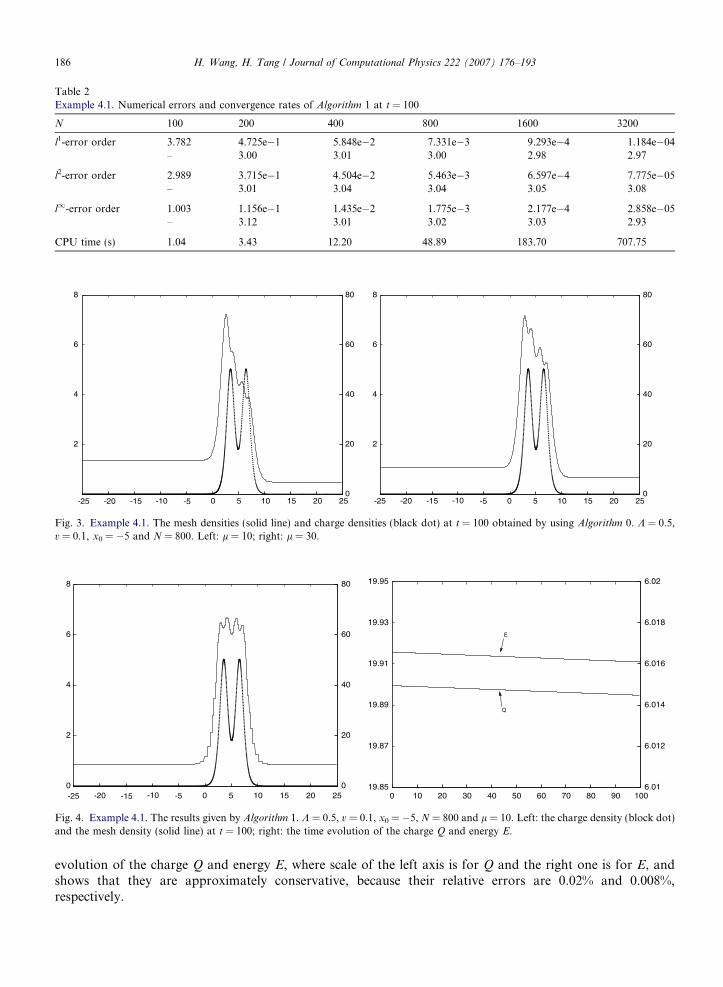
Table 2Example 4.1. Numerical errors and convergence rates of Algorithm 1 at t = 100

N 100 200 400 800 1600 3200

l1-error order 3.782 4.725e�1 5.848e�2 7.331e�3 9.293e�4 1.184e�04– 3.00 3.01 3.00 2.98 2.97



CPU time (s) 1.04 3.43 12.20 48.89 183.70 707.75

0 5 10 15 20 25

2

4

6

8

0

20

40

60

80

0 5 10 15 20 25

2

4

6

8

0

20

40

60

80

-5-10-15-20-25 -5-10-15-20-25

Fig. 3. Example 4.1. The mesh densities (solid line) and charge densities (black dot) at t = 100 obtained by using Algorithm 0. K = 0.5,v = 0.1, x0 = �5 and N = 800. Left: l = 10; right: l = 30.

0 5 10 15 20 250

2

4

6

8

0

20

40

60

80

0 10 20 30 40 50 60 70 80 90 10019.85

19.87

19.89

19.91

19.93

19.95

6.01

6.012

6.014

6.016

6.018

6.02

E

Q

-5-10-15-20-25

Fig. 4. Example 4.1. The results given by Algorithm 1. K = 0.5, v = 0.1, x0 = �5, N = 800 and l = 10. Left: the charge density (block dot)and the mesh density (solid line) at t = 100; right: the time evolution of the charge Q and energy E.


evolution of the charge Q and energy E, where scale of the left axis is for Q and the right one is for E, andshows that they are approximately conservative, because their relative errors are 0.02% and 0.008%,respectively.

010

2030 10

2550

100200

400800

0

10

20

30

40

50

60

70

80

N x

mesh density

1 0 100 200 300 400 500 600 700 8000

50

100

0.005

0.01

0.015

N1

-10-20

-30

Fig. 5. Example 4.1. Dependence of Algorithm 1 on N1. K = 0.5, v = 0.1, x0 = �5, N = 800 and t = 100. Left: the mesh density; right: theCPU time (+) and the l2-error ().

010

2030 10

2550

100200

400800

1600

0

50

100

150

Nx

mesh density

1 0 200 400 600 800 1000 1200 1400 1600100

150

200

250

300

350

N

0.5

1

1.5

2

2.5

3x 10

1

-10-20

-30

-3

Fig. 6. Example 4.1. Same as Fig. 5, except for N = 1600.


Figs. 5 and 6 give dependence of the mesh density, the CPU time (‘‘+’’, right axis) and the l2-error (‘‘’’, leftaxis) of Algorithm 1 on the parameter N1, where t = 100 and N = 800 and 1600, respectively. The results showthat the recorded CPU time and l2-error are monotonically increasing and convex functions with respect toN1, respectively; the mesh quality may be improved very well when N1 decreases properly. WhenN1 2 [25, 400], at least in the present example, Algorithm 1 is almost optimal, that is to say, its CPU timeand error are the relatively lowest, and the mesh quality is the best. It is worth noting that the optimal choiceof the parameter N1 is not too sensitive with respect to N.

Example 4.2 (Binary collisions). The second example is to investigate collisions of two one-humped solitarywaves with a phase shift of p, that is to say, we solve (1) subject to the initial data

wðx; 0Þ ¼ wssðx� xl; 0Þ � wssðx� xr; 0Þ ð33Þ
with Kl = Kr = 0.5, vl = 0.1, vr = �0.9 and xr = �xl = 10. Extensive studies of binary collisions of Dirac sol-itary waves have been conducted in [36,37]. Here we take the physical domain Xp = [�40,40], a = 10, b = 20and N = 800. For comparison, Fig. 7 gives the time evolution of the charge density qQ and the total energy E

0 10 20 30 400

5

10

15

20

25

30

35

40

45

50

0

1

2

3

0 5 10 15 20 25 30 35 40 45 506.8

6.82

6.84

6.86

6.88

6.9

6.92

6.94

6.96

6.98

7

8.6

8.61

8.62

8.63

8.64

8.65

8.66

8.67

8.68

8.69

8.7

Q

E

-10-20-30-40

Fig. 7. Example 4.2. The time evolution of the charge density qQ (left) and the total energy E and charge Q (right), obtained byAlgorithm 1.


as well as the charge Q obtained by using Algorithm 1. The results show clearly the interaction dynamics of twoDirac solitary waves, and are comparable with ones obtained by using a higher-order RKDG method on avery fine uniform mesh, see Fig. 4 in [37]. For comparison, Fig. 8 gives charge densities (black dot) and griddensities (solid line) at t = 50 obtained by using Algorithm 0 (left) and Algorithm 1 (right). We see that themesh quality of Algorithm 0 is much worse than that of Algorithm 1, because grid points clustering nearthe left peak (which is sharp) are not enough. As a result, the left peak, see left figure of Fig. 8, is lowerand moving more slowly than one in right figure. The CPU times are 140 s for Algorithm 0 and 45 s for Algo-

rithm 1, respectively. It means that about 67.86% cost is saved in the computation by using Algorithm 1.

Example 4.3 (Ternary collisions). The third example is to consider collisions of three in-phase Dirac solitarywaves. The initial data are specified as follows:

0

1

2

3

4

-40

Fig. 8

wðx; 0Þ ¼ wssðx� xl; 0Þ þ wssðx� xm; 0Þ þ wssðx� xr; 0Þ ð34Þ
with Kl = Kr = 0.9, Km = 0.1, vl = �vr = 0.9 and vm = 0. That means that the initial waves are in phase, andthe left and right waves are one-humped and the middle one is two-humped. We take the physical domainXp = [�25,25], a = b = 10 and N = 1600.
0 10 20 30 400

30

60

90

120

0 10 20 30 400

1

2

3

4

0

30

60

90

120

-10-20-30 -10-20-30-40

. Example 4.2. The charge densities (black dot) and the grid densities (solid line) at t = 50. Left: Algorithm 0; right: Algorithm 1.


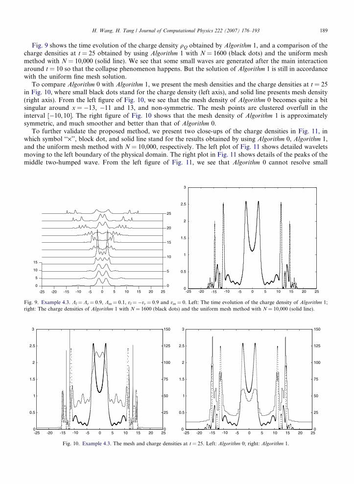
Fig. 9 shows the time evolution of the charge density qQ obtained by Algorithm 1, and a comparison of thecharge densities at t = 25 obtained by using Algorithm 1 with N = 1600 (black dots) and the uniform meshmethod with N = 10,000 (solid line). We see that some small waves are generated after the main interactionaround t = 10 so that the collapse phenomenon happens. But the solution of Algorithm 1 is still in accordancewith the uniform fine mesh solution.

To compare Algorithm 0 with Algorithm 1, we present the mesh densities and the charge densities at t = 25in Fig. 10, where small black dots stand for the charge density (left axis), and solid line presents mesh density(right axis). From the left figure of Fig. 10, we see that the mesh density of Algorithm 0 becomes quite a bitsingular around x = �13, �11 and 13, and non-symmetric. The mesh points are clustered overfull in theinterval [�10,10]. The right figure of Fig. 10 shows that the mesh density of Algorithm 1 is approximatelysymmetric, and much smoother and better than that of Algorithm 0.

To further validate the proposed method, we present two close-ups of the charge densities in Fig. 11, inwhich symbol ‘‘·’’, block dot, and solid line stand for the results obtained by using Algorithm 0, Algorithm 1,and the uniform mesh method with N = 10,000, respectively. The left plot of Fig. 11 shows detailed waveletsmoving to the left boundary of the physical domain. The right plot in Fig. 11 shows details of the peaks of themiddle two-humped wave. From the left figure of Fig. 11, we see that Algorithm 0 cannot resolve small

0 5 10 15 20 25

0

5

10

15

20

25

0

5

10

15

0 5 10 15 20 250

0.5

1

1.5

2

2.5

3

-10-20 -5-25 -15 -10-20 -5-25 -15

Fig. 9. Example 4.3. Kl = Kr = 0.9, Km = 0.1, vl = �vr = 0.9 and vm = 0. Left: The time evolution of the charge density of Algorithm 1;right: The charge densities of Algorithm 1 with N = 1600 (black dots) and the uniform mesh method with N = 10,000 (solid line).

0 5 10 15 20 250

0.5

1

1.5

2

2.5

3

0

25

50

75

100

125

150

0 5 10 15 20 250

0.5

1

1.5

2

2.5

3

0

25

50

75

100

125

150

-10-20 -5-25 -15 -10-20 -5-25 -15

Fig. 10. Example 4.3. The mesh and charge densities at t = 25. Left: Algorithm 0; right: Algorithm 1.

0

0.5

1

1.5

2

2.5Uniform meshAlgorithm 0Algorithm 1

0 1 2 3 4 52

2.1

2.2

2.3

2.4

2.5

2.6

2.7Uniform meshAlgorithm 0Algorithm 1

-18 -16 -14 -12 -10 -8 -1-2-3-4-5

Fig. 11. Example 4.3. Close up of the charge densities obtained by using Algorithm 0 (·), Algorithm 1 (Æ), and the uniform mesh methodwith N = 10,000 (solid line).


oscillatory waves. Although the mesh of Algorithm 1 in the interval [�10,10] is sparser than that ofAlgorithm 0, see Fig. 10, but their solutions are accordant in that interval, see the right figure of Fig. 11. Thus itis unnecessary to cluster too many mesh points there. Even though Algorithm 1 damps the wavelets, its resultsare in accordance with the results obtained on a uniform mesh with N = 10,000. The CPU times are 328.45 sfor Algorithm 0 and 80.60 s for Algorithm 1, respectively.

Example 4.4 (Quadruple collisions). The final example is to study quadruple collisions of the Dirac waves. Theinitial data are given as

0

1

2

-5

Fig. 121; righ

wðx; 0Þ ¼ �wssðx� xl; 0Þ þ wssðx� xlm; 0Þ þ wssðx� xrm; 0Þ � wssðx� xr; 0Þ ð35Þ
with vl = vlm = vrm = vr = 0, Kl = Kr = Klm = Krm = 0.5, xr = �xl = 15 and xrm = �xlm = 5.
We take the physical domain Xp = [�50,50], a = b = 10 and N = 1200, Fig. 12 gives the time evolution ofthe charge density qQ obtained by Algorithm 1, and a comparison of the charge densities at t = 25 obtained byusing Algorithm 1 with N = 1200 (black dots) and the uniform mesh method with N = 10,000 (solid line). Theresults show clearly the interaction dynamics of four Dirac solitary waves: four main interactions of the Dirac

0 10 20 30 40 500

50

100

150

200

250

0 10 20 30 40 500

0.2

0.4

0.6

0.8

1

1.2

1.4

-10-20-30-400 -10-20-30-40-50

. Example 4.4. vl = vlm = vrm = vr = 0 and Kl = Kr = K lm = Krm = 0.5. Left: The time evolution of the charge density of Algorithm

t: The charge densities of Algorithm 1 with N = 1200 (black dots) and the uniform mesh method with N = 10,000 (solid line).


waves happen around t = 50, 120 and 180, respectively. In connection with each main interaction, the overlaphappens, in other words, the interactions are all inelastic. The right figure of Fig. 12 shows that the solution ofAlgorithm 1 is in accord with the uniform fine mesh solution. The CPU times are 472.93 s for Algorithm 0 and79.81 s for Algorithm 1, respectively. It means that about 85.65% cost is saved in the computation by usingAlgorithm 1.

5. Remarks and conclusions

In this paper, we have proposed a highly efficient adaptive mesh method for solving the (1 + 1)-dimensionalnon-linear Dirac (NLD) equation (1). The algorithm was formed by three main parts: the NLD evolution, theiterative redistribution of the coarse mesh, and the local uniform refinement of the final coarse mesh as well asthe remapping phase of the solution vector.

At each time level, the equidistribution principle was first employed to iteratively redistribute coarse meshpoints. In the iterative coarse mesh redistribution, the scalar monitor function was interpolated on the coarsemesh instead of the solution vector, which was considered in [41]. After the final adaptive coarse mesh wasgenerated ideally, each coarse mesh interval was equally divided into some uniform fine cells to give the adap-tive fine mesh of the physical domain. Then the solution vector was remapped from the old fine mesh to thenew fine mesh by marching the remapping solver forward in the parameter or pseudo-time by one unit stepsize. Finally, the governing equations were solved by using a high resolution shock-capturing method overa fixed quadrate control volume in the space and time domain. Our proposed method may be consideredas a combination of the r-refinement method and the h-refinement method and shares the same idea of thetwo-level mesh movement technique of Huang et al. [23,24] and Fiedler and Trapp [20] as well as the hr-refine-ment method in the literatures.

Extensive numerical experiments have been presented to demonstrate that the proposed adaptive meshmethod is much more efficient and faster than the method of [41], may give third-order rates of convergenceand yields a powerful and fast NLD solver that tracks and resolves both small, local and large solution gra-dients automatically. It is worth noting that quadruple collisions of the Dirac solitary waves are studied for thefirst time.

In future, we will extend the present method to multidimensional Dirac model and conduct research in the-oretical and applied analysis of the adaptive mesh methods.

Acknowledgments

This research was partially supported by the National Basic Research Program under the Grant2005CB321703, the National Natural Science Foundation of China (No. 10431050, 10576001), and Labo-ratory of Computational Physics. HZT would like to thank Mr. Sihong Shao for numerous discussions dur-ing the preparation of this work. We would also like to thank anonymous referees for many helpfulsuggestions.

References

[1] S. Adjerid, J.E. Flaherty, A moving-mesh finite element method with local refinement for parabolic partial differential equations,Comput. Methods Appl. Mech. Eng. 55 (1986) 3–26.

[2] S. Adjerid, J.E. Flaherty, A moving finite element method with error estimation and refinement for one-dimensional time dependentpartial differential equations, SIAM J. Numer. Anal. 23 (1986) 778–796.

[3] A. Alvarez, Linearized Crank–Nicholson scheme for nonlinear Dirac equations, J. Comput. Phys. 99 (1992) 348–350.[4] A. Alvarez, Spinorial solitary wave dynamics of a (1 + 3)-dimensional model, Phys. Rev. D 31 (1985) 2701–2703.[5] A. Alvarez, B. Carreras, Interaction dynamics for the solitary waves of a nonlinear Dirac model, Phys. Lett. A 86 (1981) 327–

332.[6] A. Alvarez, A.F. Randa, Blow-up in nonlinear models of extended particles with confined constituents, Phys. Rev. D 38 (1988) 3330–

3333.[7] A. Alvarez, M. Soler, Energetic stability criterion for a nonlinear spinorial model, Phys. Rev. Lett. 50 (1983) 1230–1233.[8] A. Alvarez, M. Soler, Stability of the minimum solitary wave of a nonlinear spinorial model, Phys. Rev. D 34 (1986) 644–645.


[9] B.N. Azarenok, S.A. Ivanenko, T. Tang, Adaptive mesh redistribution method based on Godunov’s scheme, Commun. Math. Sci. 1(2003) 152–179.

[10] G. Beckett, J.A. Mackenzie, M.L. Robertson, An r-adaptive finite element method for the solution of the two-dimensional phase-fieldequations, Commun. Comput. Phys. 1 (2006) 805–826.

[11] J.U. Brackbill, An adaptive grid with directional control, J. Comput. Phys. 108 (1993) 38–50.[12] J.U. Brackbill, J.S. Saltzman, Adaptive zoning for singular problems in two dimensions, J. Comput. Phys. 46 (1982) 342–368.[13] W.M. Cao, W.Z. Huang, R.D. Russell, A study of monitor functions for two-dimensional adaptive mesh generation, SIAM J. Sci.

Comput. 20 (1999) 1978–1999.[14] W.M. Cao, W.Z. Huang, R.D. Russell, An r-adaptive finite element method based upon moving mesh PDEs, J. Comput. Phys. 149

(1999) 221–244.[15] H.D. Ceniceros, T.Y. Hou, An efficient dynamically adaptive mesh for potentially singular solutions, J. Comput. Phys. 172 (2001)

609–639.[16] S.F. Davis, J.E. Flaherty, An adaptive finite element method for initial-boundary value problems for partial differential equations,

SIAM J. Sci. Stat. Comput. 3 (1982) 6–27.[17] J. De Frutos, J.M. Sanz-serna, Split-step spectral schemes for nonlinear Dirac systems, J. Comput. Phys. 83 (1989) 407–423.[18] A.S. Dvinsky, Adaptive grid generation from harmonic maps on Riemannian manifolds, J. Comput. Phys. 95 (1991) 450–476.[19] R. Fazio, R. LeVeque, Moving-mesh methods for one-dimensional hyperbolic problems using CLAWPACK, Comp. Math. Appl. 45

(2003) 273–298.[20] B.H. Fiedler, R.J. Trapp, A fast dynamic grid adaption scheme for meteorological flows, Mon. Weather Rev. 121 (1993) 2879–2888.[21] A. Harten, J.M. Hyman, Self-adjusting grid methods for one-dimensional hyperbolic conservation laws, J. Comput. Phys. 50 (1983)

235–269.[22] J.L. Hong, C. Li, Multi-symplectic Runge–Kutta methods for nonlinear Dirac equations, J. Comput. Phys. 211 (2006) 448–472.[23] W.Z. Huang, Practical aspects of formulation and solution of moving mesh partial differential equations, J. Comput. Phys. 171 (2001)

753–755.[24] J. Lang, W.M. Cao, W.Z. Huang, R.D. Russell, A two-dimensional moving finite element method with local refinement based on a

posteriori error estimates, Appl. Numer. Math. 46 (2003) 75–94.[25] R. Li, T. Tang, P.W. Zhang, Moving mesh methods in multiple dimensions based on harmonic maps, J. Comput. Phys. 170 (2001)

562–588.[26] R. Li, T. Tang, P.W. Zhang, A moving mesh finite element algorithm for singular problems in two and three space dimensions, J.

Comput. Phys. 177 (2002) 365–393.[27] S. Li, L. Petzold, Moving mesh methods with upwinding schemes for time-dependent PDEs, J. Comput. Phys. 131 (1997) 368–377.[28] F. Liu, S. Ji, G. Liao, An adaptive grid method and its application to steady Euler flow calculations, SIAM J. Sci. Comput. 20 (1998)

811–825.[29] K. Miller, R.N. Miller, Moving finite element. I, SIAM J. Numer. Anal. 18 (1981) 1019–1032.[30] J.T. Oden, T. Strouboulis, P. Devloo, Adaptive finite element methods for the analysis of inviscid compressible flow. I. Fast

refinement/unrefinement and moving mesh methods for unstructured meshes, Comput. Methods Appl. Mech. Eng. 59 (1986) 327–362.

[31] A.F. Ranada, M. Soler, Perturbation theory for an exactly soluble spinor model in interaction with its electromagnetic field, Phys.Rev. D 8 (1973) 3430–3433.

[32] A.F. Ranada, M.F. Ranada, M. Soler, L. Vazquez, Classical electrodynamics of a nonlinear Dirac field with anomalous magneticmoment, Phys. Rev. D 10 (1974) 517–525.

[33] W.Q. Ren, X.P. Wang, An iterative grid redistribution method for singular problems in multiple dimensions, J. Comput. Phys. 159(2000) 246–273.

[34] K. Saleri, S. Steinberg, Flux-corrected transport in a moving grid, J. Comput. Phys. 111 (1994) 24–32.[35] S.H. Shao, H.Z. Tang, Higher-order accurate Runge–Kutta discontinuous Galerkin methods for a nonlinear Dirac model, Discrete

Cont. Dyn. Syst. Ser. B 6 (2006) 623–640.[36] S.H. Shao, H.Z. Tang, Interaction for the solitary waves of a nonlinear Dirac model, Phys. Lett. A 345 (2005) 119–128.[37] S.H. Shao, H.Z. Tang, Interaction for solitary waves with a phase difference in a nonlinear Dirac model, ArXiv: nlin.SI/0604033v1,

2006. Available from: <http://arxiv.org/pdf/nlin.SI/0604033>.[38] M. Soler, Classical, stable, nonlinear spinor field with positive rest energy, Phys. Rev. D 1 (1970) 2766–2769.[39] J.M. Stockie, J.A. Mackenzie, R.D. Russell, A moving mesh method for one-dimensional hyperbolic conservation laws, SIAM J. Sci.

Comput. 22 (2001) 1791–1813.[40] H.Z. Tang, T. Tang, Multi-dimensional moving mesh methods for shock computations, Contemp. Math. 330 (2003) 169–183.[41] H.Z. Tang, T. Tang, Adaptive mesh methods for one- and two-dimensional hyperbolic conservation laws, SIAM J. Numer. Anal. 41

(2003) 487–515.[42] H.Z. Tang, T. Tang, P.W. Zhang, An adaptive mesh redistribution method for nonlinear Hamilton–Jacobi equations in two- and

three-dimensions, J. Comput. Phys. 188 (2003) 534–572.[43] T. Tang, Moving mesh methods for computational fluid dynamics, Contemp. Math. 383 (2005) 141–174.[44] B. van Leer, Towards the ultimate conservative difference scheme, V. A second order sequel to Godunov’s method, J. Comput. Phys.

32 (1979) 101–136.[45] D.S. Wang, X.P. Wang, A three-dimensional adaptive method based on the iterative grid redistribution, J. Comput. Phys. 199 (2004)

423–436.

http://arxiv.org/pdf/nlin.SI/0604033


[46] Z.-Q. Wang, B.-Y. Guo, Modified Legendre rational spectral method for the whole line, J. Comput. Math. 22 (2004) 457–474.[47] A. Winslow, Numerical solution of the quasi-linear Poisson equation, J. Comput. Phys. 1 (1967) 149–172.[48] P.A. Zegeling, On resistive MHD models with adaptive moving meshes, J. Sci. Comput. 24 (2005) 263–284.[49] P.A. Zegeling, W.D. de Boer, H.Z. Tang, Robust and efficient adaptive moving mesh solution of the 2-D Euler equations, Contemp.

Math. 383 (2005) 375–386.[50] Z.R. Zhang, Moving mesh method with conservative interpolation based on L2-projection, Commun. Comput. Phys. 1 (2006) 930–

944.

an efficient adaptive mesh redistribution method for a non-linear dirac equation

Documents