an efficient and stable numerical method for the maxwell–dirac system
TRANSCRIPT

Journal of Computational Physics 199 (2004) 663–687
www.elsevier.com/locate/jcp
An efficient and stable numerical method forthe Maxwell–Dirac system
Weizhu Bao *, Xiang-Gui Li
Department of Computational Science, National University of Singapore, Singapore 117543, Singapore
Received 14 January 2004; received in revised form 27 February 2004; accepted 9 March 2004
Available online 12 April 2004
Abstract
In this paper, we present an explicit, unconditionally stable and accurate numerical method for the Maxwell–Dirac
system (MD) and use it to study dynamics of MD. As preparatory steps, we take the three-dimensional (3D) Maxwell–
Dirac system, scale it to obtain a two-parameter model and review plane wave solution of free MD. Then we present a
time-splitting spectral method (TSSP) for MD. The key point in the numerical method is based on a time-splitting
discretization of the Dirac system, and to discretize nonlinear wave-type equations by pseudospectral method for spatial
derivatives, and then solving the ordinary differential equations (ODEs) in phase space analytically under appropriate
chosen transmission conditions between different time intervals. The method is explicit, unconditionally stable, time
reversible, time transverse invariant, and of spectral-order accuracy in space and second-order accuracy in time.
Moreover, it conserves the particle density exactly in discretized level and gives exact results for plane wave solution of
free MD. Extensive numerical tests are presented to confirm the above properties of the numerical method. Further-
more, the tests also suggest the following meshing strategy (or e-resolution) is admissible in the ‘nonrelativistic’ limit
regime (0 < e � 1): spatial mesh size h ¼ OðeÞ and time step 4t ¼ Oðe2Þ, where the parameter e is inversely propor-
tional to the speed of light.
� 2004 Elsevier Inc. All rights reserved.
Keywords: Maxwell–Dirac system; Time-splitting spectral method; Unconditionally stable; Time reversible; Semiclassical; Plane wave
1. Introduction
One of the fundamental quantum-relativistic equations is given by the Maxwell–Dirac system (MD), i.e.
the Dirac equation [16,28] for the electron as a spinor coupled to the Maxwell equations for the electro-magnetic field. It represents the time-evolution of fast (relativistic) electrons and positrons within self-
consistent generated electromagnetic fields. In its most compact form, the Dirac equation reads [8,17,23,27]
*Corresponding author. Tel.: +65-6874-3337; fax: +65-6774-6756.
E-mail addresses: [email protected] (W. Bao), [email protected] (X.-G. Li).
URL: http://www.cz3.nus.edu.sg/~bao/.
0021-9991/$ - see front matter � 2004 Elsevier Inc. All rights reserved.
doi:10.1016/j.jcp.2004.03.003

664 W. Bao, X.-G. Li / Journal of Computational Physics 199 (2004) 663–687
i�hcgog�
� m0cþ ecgAg
�W ¼ 0: ð1:1Þ
Here the unknown W is the 4-vector complex wave function of the ‘‘spinorfield’’: Wðt; xÞ ¼ðW1;W2;W3;W4ÞT 2 C4, x0 ¼ ct, x ¼ ðx1; x2; x3ÞT 2 R3 with x0; x denoting the time – resp. spatial coordinates
in Minkowski space. og stands forooxg, i.e. o0 ¼ o
ox0¼ 1
coot, ok ¼ o
oxkðk ¼ 1; 2; 3Þ, where we consequently adopt
notation that Greek letter g denotes 0, 1, 2, 3 and k denotes the three spatial dimension indices 1, 2, 3. cgAg
stands for the summationP3
g¼0 cgAg. The physical constants are: �h for the Planck constant, c for the speed
of light, m0 for the electron’s rest mass, and e for the unit charge. By cg 2 C4�4, g ¼ 0; . . . ; 3, we denote the4� 4 Dirac matrices given by
c0 ¼ I2 0
0 �I2
� �; ck ¼ 0 rk
�rk 0
� �; k ¼ 1; 2; 3;
where Im (m a positive integer) is the m� m identity matrix and rk ðk ¼ 1; 2; 3Þ the 2� 2 Pauli matrices, i.e.
r1 :¼ 0 1
1 0
� �; r2 :¼ 0 �i
i 0
� �; r3 :¼ 1 0
0 �1
� �:
Agðt; xÞ 2 R, g ¼ 0; . . . ; 3, are the components of the time-dependent electromagnetic potential, in partic-
ular V ðt; xÞ ¼ �A0ðt; xÞ is the electric potential and Aðt; xÞ ¼ ðA1;A2;A3ÞT is the magnetic potential vector.
Hence the electric and magnetic fields are given by
Eðt; xÞ ¼ rA0 � otA ¼ �rV � otA; Bðt; xÞ ¼ curlA ¼ r� A: ð1:2Þ
In order to determine the electric and magnetic potentials from fields uniquely, we have to choose a gauge.
In practice, the Lorentz gauge condition is often introduced
Lðt; xÞ :¼ 1
cotV þr � A ¼ � 1
cotA0 þr � A ¼ 0: ð1:3Þ
Thus the electric and magnetic fields are governed by the Maxwell equation:
� 1
cotEþr� B ¼ 1
c�0J; r � B ¼ 0; ð1:4Þ
1
cotBþr� E ¼ 0; r � E ¼ 1
�0q; ð1:5Þ
where �0 is the permittivity of the free space. The particle density q and current density J ¼ ðj1; j2; j3ÞT aredefined as follows:
q ¼ ejWj2 :¼ eX4
j¼1
jWjj2; jk ¼ echW; akWi :¼ ec �WTakW; k ¼ 1; 2; 3; ð1:6Þ
where �f denotes the conjugate of f and
ak ¼ c0ck ¼ 0 rk
rk 0
� �; k ¼ 1; 2; 3: ð1:7Þ
From now on, we adopt the standard notations j � j, h�; �i and k � k for l2-norm of a vector, inner product
and L2-norm of a function.

W. Bao, X.-G. Li / Journal of Computational Physics 199 (2004) 663–687 665
Separating the time derivative associated to the ‘‘relativistic time variable’’ x0 ¼ ct and applying c0 fromleft of (1.1), plugging (1.2) into (1.4) and (1.5), noticing (1.3), we have the following Maxwell–Dirac system
[26]
i�hotW ¼X3
k¼1
akð � i�hcok � eAkÞWþ eVWþ m0c2bW; ð1:8Þ
1
c2o2t
�� D
�V ¼ 1
�0q;
1
c2o2t
�� D
�A ¼ 1
c�0J: ð1:9Þ
The vector wave function W is normalized as
kWðt; �Þk2 :¼ZR3
jWðt; xÞj2 dx ¼ 1: ð1:10Þ
The MD system (1.8) and (1.9) represents the time-evolution of fast (relativistic) electrons and positrons
within self-consistent generated electromagnetic fields. From the mathematical point of view, the strongly
nonlinear MD system poses a hard problem in the study of PDEs arising from quantum physics. Wellposedness and existence of solutions on all of R3 but only locally in time has been proved almost 40 years
ago [11,12,21]. In particular, there are no global existence results without smallness assumptions on the
initial data [19,20]. Thus the MD system is quite involved from the numerical point of view as it poses major
open problems from analytical point of view. For solitary solution of MD, we refer [1,10,13,14,23].
The aim of this paper is to design an explicit, unconditionally stable and accurate numerical method for
the MD system and apply it to study dynamics of MD. The key point in the numerical method is based on a
time-splitting discretization of the Dirac system (1.8), which was used successfully to solve nonlinear
Schr€odinger equation (NLS) [2–5] and Zakharov system [6,7], and to discretize the nonlinear wave-typeequation (1.9) by pseudospectral method for spatial derivatives, and then solving the ODEs in phase space
analytically under appropriate chosen transmission conditions between different time intervals.
The paper is organized as follows. In Section 2, we start out with the MD, scale it to get a two-parameter
model and review plane wave solution of free MD. In Section 3, we present a time-splitting spectral method
(TSSP) for the MD and show some properties of the numerical method. In Section 4, numerical tests of
MD for different cases are reported to demonstrate efficiency and high resolution of our numerical method.
In Section 5 a summary is given.
2. The Maxwell–Dirac system
Consider the Maxwell–Dirac system represents the time-evolution of fast (relativistic) electrons and
positrons within external and self-consistent generated electromagnetic fields [26]
i�hotW ¼X3
k¼1
ak�� i�hcok � e Ak
�þ Aext
k
��Wþ e Vð þ V extÞWþ m0c2bW; ð2:1Þ
1
c2o2t
�� D
�V ¼ 1
�0q;
1
c2o2t
�� D
�A ¼ 1
c�0J; ð2:2Þ

666 W. Bao, X.-G. Li / Journal of Computational Physics 199 (2004) 663–687
where V ext ¼ V extðt; xÞ 2 R and Aextðt; xÞ ¼ ðAext1 ;Aext
2 ;Aext3 ÞT 2 R3 are the external electric and magnetic
potentials, respectively.
2.1. Dimensionless Maxwell–Dirac system
We rescale the MD (2.1) and (2.2) under the normalization (1.10) by introducing a reference velocity v,length L ¼ e2=m0v2�0, time T ¼ v=L, and strength of the electromagnetic potential k ¼ e=L�0, as
~x ¼ x
L; ~t ¼ t
T; ~Wð~t; ~xÞ ¼ L3=2Wðt; xÞ; ~V ð~t; ~xÞ ¼ kV ðt; xÞ; ð2:3Þ
~Að~t; ~xÞ ¼ kAðt; xÞ; ~Aextð~t; ~xÞ ¼ kAextðt; xÞ; ~V extð~t; ~xÞ ¼ kV extðt; xÞ: ð2:4Þ
Plugging (2.3) and (2.4) into (2.1) and (2.2), then removing all �, we get the following dimensionless MD:
idotW ¼ �ide
X3
k¼1
akokW�X3
k¼1
akðAk þ Aextk ÞWþ ðV þ V extÞWþ 1
e2bW; ð2:5Þ
e2o2t�
� D�V ¼ q; e2o2t
�� D
�A ¼ eJ: ð2:6Þ
Two important dimensionless parameters in the MD (2.5) and (2.6) are given by the ratio of the referencevelocity to the speed of light, i.e. e, and the scaled Planck constant, i.e. d, as
e :¼ vc; d :¼ �h�0v
e2: ð2:7Þ
The position and current densities, Lorentz gauge, as well as electric and magnetic fields in dimensionless
variables are
qðt; xÞ ¼ jWðt; xÞj2; jkðt; xÞ ¼1
ehWðt; xÞ; akWðt; xÞi; k ¼ 1; 2; 3; ð2:8Þ
Lðt; xÞ ¼ eotV ðt; xÞ þ r � Aðt; xÞ; tP 0; x 2 R3; ð2:9ÞEðt; xÞ ¼ �eotAðt; xÞ � rV ðt; xÞ; Bðt; xÞ ¼ r � Aðt; xÞ: ð2:10Þ
When v � c and choosing v ¼ c, then e ¼ 1 in (2.7) and the MD (2.5) and (2.6) collapse to a one-parameter
model which is used in [26] to study classical limit and semiclassical asymptotics of MD. In this case, theparameter d is the same as the canonical parameter a used in physical literatures [16,28]. When v � c and
choosing v ¼ e2=�h�0, then d ¼ 1 and 0 < e � 1 in (2.7), again the MD (2.5) and (2.6) collapse to a one-
parameter model which is called as ‘nonrelativistic’ limit regime and used in [8,9,18,22,24,25] to study semi-
nonrelativistic limits of MD, i.e. letting e ! 0 in (2.5) and (2.6). For electrons, e ¼ 1 and d � 10:9149 [26].
The MD system (2.5) and (2.6) together with initial data
Wð0; xÞ ¼ Wð0ÞðxÞ with kWð0Þk ¼ZR3
jWð0ÞðxÞj2 dx ¼ 1; ð2:11Þ
V ð0; xÞ ¼ V ð0ÞðxÞ; otV ð0; xÞ ¼ V ð1ÞðxÞ; x 2 R3; ð2:12Þ
Að0; xÞ ¼ Að0ÞðxÞ; otAð0; xÞ ¼ Að1ÞðxÞ ð2:13Þ
W. Bao, X.-G. Li / Journal of Computational Physics 199 (2004) 663–687 667
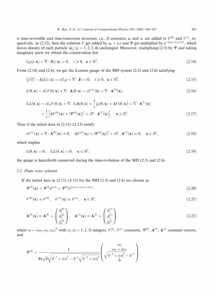
is time-reversible and time-transverse invariant, i.e., if constants a0 and a1 are added to V ð0Þ and V ð1Þ, re-
spectively, in (2.12), then the solution V get added by a0 þ a1t and W get multiplied by e�itða0þa1t=2Þ=d, which
leaves density of each particle jwjj (j ¼ 1; 2; 3; 4) unchanged. Moreover, multiplying (2.5) by �W and takingimaginary parts we obtain the conservation law
otqðt; xÞ þ r � Jðt; xÞ ¼ 0; tP 0; x 2 R3: ð2:14Þ
From (2.14) and (2.6), we get the Lorentz gauge of the MD system (2.5) and (2.6) satisfying
e2o2t�
� D�Lðt; xÞ ¼ e otqð þ r � JÞ ¼ 0; tP 0; x 2 R3; ð2:15Þ
Lð0; xÞ ¼ eotV ð0; xÞ þ r � Að0; xÞ ¼ eV ð1ÞðxÞ þ r � Að0ÞðxÞ; ð2:16Þ
otLð0; xÞ ¼ eottV ð0; xÞ þ r � otAð0; xÞ ¼1
eqð0; xÞ½ þ DV ð0; xÞ� þ r � Að1ÞðxÞ
¼ 1
eDV ð0ÞðxÞh
þ jWð0ÞðxÞj2 þ er � Að1ÞðxÞi; x 2 R3: ð2:17Þ
Thus if the initial data in (2.11)–(2.13) satisfy
eV ð1ÞðxÞ þ r � Að0ÞðxÞ � 0; DV ð0ÞðxÞ þ jWð0ÞðxÞj2 þ er � Að1ÞðxÞ � 0; x 2 R3; ð2:18Þ
which implies
Lð0; xÞ ¼ 0; otLð0; xÞ ¼ 0; x 2 R3; ð2:19Þ
the gauge is henceforth conserved during the time-evolution of the MD (2.5) and (2.6).
2.2. Plane wave solution
If the initial data in (2.11)–(2.13) for the MD (2.5) and (2.6) are chosen as
Wð0ÞðxÞ ¼ Wð0Þeix�x ¼ Wð0Þeiðx1x1þx2x2þx3x3Þ; ð2:20Þ
V ð0ÞðxÞ � V ð0Þ; V ð1ÞðxÞ � V ð1Þ; x 2 R3; ð2:21Þ
Að0ÞðxÞ � Að0Þ ¼Að0Þ1
Að0Þ2
Að0Þ3
0B@1CA; Að1ÞðxÞ � Að1Þ ¼
Að1Þ1
Að1Þ2
Að1Þ3
0B@1CA; ð2:22Þ
where x ¼ ðx1;x2;x3ÞT with xj (j ¼ 1; 2; 3) integers, V ð0Þ, V ð1Þ constants, Wð0Þ, Að0Þ, Að1Þ constant vectors,
and
Wð0Þ ¼ 1
4pffiffiffip
pffiffiffiffiffiffiffiffiffiffiffiffiffiffiffiffiffiffiffiffiffiffiffiffiffiffiffiffiffiffiffiffiffiffiffiffiffiffiffiffiffiffiffiffiffiffiffiffiffiffiffiffiffiffiffiffiffiffid�2 þ jxj2 � d�1
ffiffiffiffiffiffiffiffiffiffiffiffiffiffiffiffiffiffiffiffiffid�2 þ jxj2
qrx3
x1 þ ix2ffiffiffiffiffiffiffiffiffiffiffiffiffiffiffiffiffiffiffiffiffid�2 þ jxj2
q� d�1
0
0BB@1CCA;

668 W. Bao, X.-G. Li / Journal of Computational Physics 199 (2004) 663–687
then the MD (2.5) and (2.6) with e ¼ 1, Aext ¼ �A and V ext ¼ �V , i.e. free MD [15], admits the following
plane wave solution:
Wðt; xÞ ¼ Wð0Þ exp ix � x�
� itffiffiffiffiffiffiffiffiffiffiffiffiffiffiffiffiffiffiffiffiffid�2 þ jxj2
q �; ð2:23Þ
V ðt; xÞ ¼ �V ext ¼ V ð0Þ þ V ð1Þt þ 1
16p3t2; x 2 R3; tP 0; ð2:24Þ
Aðt; xÞ ¼ �Aext ¼ Að0Þ þ Að1Þt þ 1
2Jð0Þt2; ð2:25Þ
where Jð0Þ ¼ ðjð0Þ1 ; jð0Þ2 ; jð0Þ3 ÞT and
jð0Þk ¼ xk
8p3
ffiffiffiffiffiffiffiffiffiffiffiffiffiffiffiffiffiffiffiffiffid�2 þ jxj2
q ; k ¼ 1; 2; 3:
Here the normalization condition for the wave function is set asZ p
�p
Z p
�p
Z p
�pjWðt; xÞj2 dx ¼ 1:
3. Numerical method
In this section we present an explicit, unconditionally stable and accurate numerical method for the MD
(2.5) and (2.6). We shall introduce the method in 3D on a box with periodic boundary conditions. For 3D
in a box X ¼ ½a1; b1� � ½a2; b2� � ½a3; b3�, the problem with initial and boundary conditions become
idotW ¼ �ide
X3
k¼1
akokW�X3
k¼1
akðAk þ Aextk ÞWþ ðV þ V extÞWþ 1
e2bW; ð3:1Þ
e2o2t�
� D�V ðt; xÞ ¼ q; e2o2t
�� D
�Aðt; xÞ ¼ eJ; x 2 X; t > 0; ð3:2Þ
Wð0; xÞ ¼ Wð0ÞðxÞ; V ð0; xÞ ¼ V ð0ÞðxÞ; otV ð0; xÞ ¼ V ð1ÞðxÞ; ð3:3Þ
Að0; xÞ ¼ Að0ÞðxÞ; otAð0; xÞ ¼ Að1ÞðxÞ; x 2 X ð3:4Þ
with periodic boundary conditions for W; V ;A on oX; ð3:5Þ
where V ð1Þ and Að0Þ satisfy
eV ð1ÞðxÞ þ r � Að0ÞðxÞ ¼ 0; x 2 X ð3:6Þ
and the normalization condition for the wave function is set as
kWðt; �Þk2 :¼ZXjWðt; xÞj2 dx ¼
ZXjWð0ÞðxÞj2 dx ¼ 1: ð3:7Þ
W. Bao, X.-G. Li / Journal of Computational Physics 199 (2004) 663–687 669
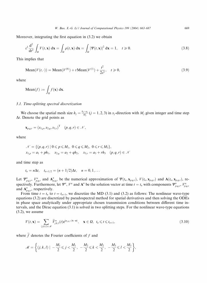
Moreover, integrating the first equation in (3.2) we obtain
e2d2
dt2
ZXV ðt; xÞ dx ¼
ZXqðt; xÞ dx ¼
ZXjWðt; xÞj2 dx ¼ 1; tP 0: ð3:8Þ
This implies that
MeanðV ðt; �ÞÞ ¼ MeanðV ð0ÞÞ þ tMeanðV ð1ÞÞ þ t2
2e2; tP 0; ð3:9Þ
where
Meanðf Þ :¼ZXf ðxÞ dx:
3.1. Time-splitting spectral discretization
We choose the spatial mesh size hj ¼ bj�ajMj
(j ¼ 1; 2; 3) in xj-direction with Mj given integer and time step
Dt. Denote the grid points as
xp;q;r ¼ ðx1;p; x2;q; x3;rÞT ðp; q; rÞ 2 N;
where
N ¼ ðp; q; rÞ j 0f 6 p6M1; 06 q6M2; 06 r6M3g;x1;p ¼ a1 þ ph1; x2;q ¼ a2 þ qh2; x3;r ¼ a3 þ rh3 ðp; q; rÞ 2 N
and time step as
tn ¼ nDt; tnþ1=2 ¼ ðnþ 1=2ÞDt; n ¼ 0; 1; . . .
Let Wnp;q;r, V
np;q;r and An
p;q;r be the numerical approximation of Wðtn; xp;q;rÞ, V ðtn; xp;q;rÞ and Aðtn; xp;q;rÞ, re-spectively. Furthermore, let Wn, V n and An be the solution vector at time t ¼ tn with components Wn
p;q;r, Vnp;q;r
and Anp;q;r, respectively.
From time t ¼ tn to t ¼ tnþ1, we discretize the MD (3.1) and (3.2) as follows: The nonlinear wave-type
equations (3.2) are discretized by pseudospectral method for spatial derivatives and then solving the ODEs
in phase space analytically under appropriate chosen transmission conditions between different time in-tervals, and the Dirac equation (3.1) is solved in two splitting steps. For the nonlinear wave-type equations
(3.2), we assume
V ðt; xÞ ¼X
ðj;k;lÞ2M
eV nj;k;lðtÞeilj;k;l�ðx�aÞ; x 2 X; tn 6 t6 tnþ1; ð3:10Þ
where ef denotes the Fourier coefficients of f and
M ¼ ðj; k; lÞ j�
�M1
26 j <
M1
2; �M2
26 k <
M2
2; �M3
26 l <
M3
2
;
670 W. Bao, X.-G. Li / Journal of Computational Physics 199 (2004) 663–687
lj;k;l ¼lð1Þj
lð2Þk
lð3Þl
0B@1CA; a ¼
a1a2a3
0@ 1Awith
lð1Þj ¼ 2pj
b1 � a1; lð2Þ
k ¼ 2pkb2 � a2
; lð3Þl ¼ 2pl
b3 � a3; ðj; k; lÞ 2 M:
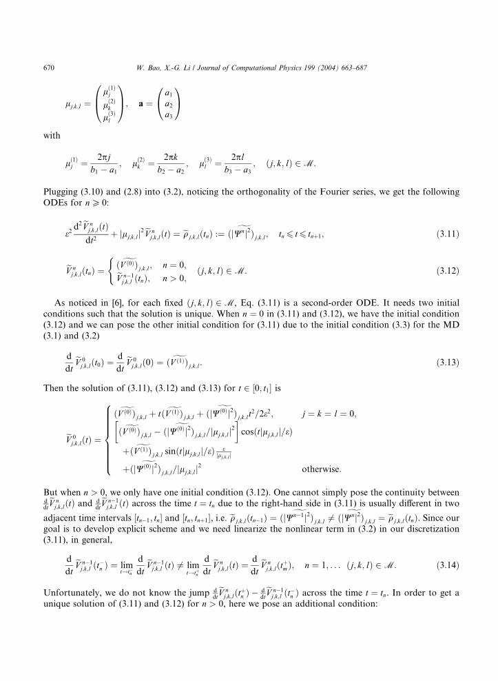
Plugging (3.10) and (2.8) into (3.2), noticing the orthogonality of the Fourier series, we get the following
ODEs for nP 0:
e2d2 eV n
j;k;lðtÞdt2
þ jlj;k;lj2 eV n
j;k;lðtÞ ¼ eqj;k;lðtnÞ :¼gðjWnj2Þj;k;l; tn 6 t6 tnþ1; ð3:11Þ
eV nj;k;lðtnÞ ¼
gðV ð0ÞÞj;k;l; n ¼ 0;eV n�1j;k;l ðtnÞ; n > 0;
(ðj; k; lÞ 2 M: ð3:12Þ
As noticed in [6], for each fixed ðj; k; lÞ 2 M, Eq. (3.11) is a second-order ODE. It needs two initial
conditions such that the solution is unique. When n ¼ 0 in (3.11) and (3.12), we have the initial condition
(3.12) and we can pose the other initial condition for (3.11) due to the initial condition (3.3) for the MD
(3.1) and (3.2)
d
dteV 0j;k;lðt0Þ ¼
d
dteV 0j;k;lð0Þ ¼ gðV ð1ÞÞj;k;l: ð3:13Þ
Then the solution of (3.11), (3.12) and (3.13) for t 2 ½0; t1� is
eV 0j;k;lðtÞ ¼
gðV ð0ÞÞj;k;l þ t gðV ð1ÞÞj;k;l þgðjWð0Þj2Þj;k;lt2=2e2; j ¼ k ¼ l ¼ 0;gðV ð0ÞÞj;k;l �
gðjWð0Þj2Þj;k;l=jlj;k;lj2
�cosðtjlj;k;lj=eÞ
þ gðV ð1ÞÞj;k;l sinðtjlj;k;lj=eÞ ejlj;k;lj
þ gðjWð0Þj2Þj;k;l=jlj;k;lj2
otherwise:
8>>>>>>><>>>>>>>:But when n > 0, we only have one initial condition (3.12). One cannot simply pose the continuity betweenddteV nj;k;lðtÞ and d
dteV n�1j;k;l ðtÞ across the time t ¼ tn due to the right-hand side in (3.11) is usually different in two
adjacent time intervals ½tn�1; tn� and ½tn; tnþ1�, i.e. eqj;k;lðtn�1Þ ¼ gðjWn�1j2Þj;k;l 6¼gðjWnj2Þj;k;l ¼ eqj;k;lðtnÞ. Since our
goal is to develop explicit scheme and we need linearize the nonlinear term in (3.2) in our discretization
(3.11), in general,
d
dteV n�1j;k;l ðt�n Þ ¼ lim
t!t�n
d
dteV n�1j;k;l ðtÞ 6¼ lim
t!tþn
d
dteV nj;k;lðtÞ ¼
d
dteV nj;k;lðtþmÞ; n ¼ 1; . . . ðj; k; lÞ 2 M: ð3:14Þ
Unfortunately, we do not know the jump ddteV nj;k;lðtþn Þ � d
dteV n�1j;k;l ðt�n Þ across the time t ¼ tn. In order to get a
unique solution of (3.11) and (3.12) for n > 0, here we pose an additional condition:

W. Bao, X.-G. Li / Journal of Computational Physics 199 (2004) 663–687 671
eV nj;k;lðtn�1Þ ¼ eV n�1
j;k;l ðtn�1Þ ðj; k; lÞ 2 M: ð3:15Þ
The condition (3.15) is equivalent to pose the solution eV nj;k;lðtÞ on the time interval ½tn; tnþ1� of (3.11) and
(3.12) is also continuity at the time t ¼ tn�1. After a simple computation, we get the solution of (3.11), (3.12)
and (3.15) for n > 0
eV nj;k;lðtÞ ¼
eV nj;k;lðtnÞ þ eqj;k;lðtnÞðt � tnÞ2=2e2
þ t�tnDt
eV nj;k;lðtnÞ � eV n�1
j;k;l ðtn�1Þ þ eqj;k;lðtnÞðDtÞ2=2e2
h i; j ¼ k ¼ l ¼ 0;eV n
j;k;l � eqj;k;lðtnÞ=jlj;k;lj2
h icosððt � tnÞjlj;k;lj=eÞ
þ ð1� cosðjlj;k;ljDt=eÞÞeqj;k;lðtnÞ=jlj;k;lj2 � eV n�1
j;k;l ðtn�1Þh
þeV nj;k;lðtnÞ cosðjlj;k;ljDt=eÞ
isinððt�tnÞjlj;k;lj=eÞsinðjlj;k;ljDt=eÞ
þeqj;k;lðtnÞ=jlj;k;lj2
otherwise:
8>>>>>>>>>>><>>>>>>>>>>>:Discretization for the equation of A in (3.2) can be done in a similar way.
For the Dirac equation (3.1), we solve it in two splitting steps. One solves first
idotWðt; xÞ ¼ �ide
X3
k¼1
akokWþ 1
e2bW; x 2 X; tn 6 t6 tnþ1 ð3:16Þ
for the time step of length Dt, followed by solving
idotWðt; xÞ ¼ ðV þ V extÞW�X3
k¼1
akðAk þ Aextk ÞW ¼ Gðt; xÞW ð3:17Þ
for the same time step with
Gðt; xÞ ¼ V ðt; xÞð"
þ V extðt; xÞÞI4 �X3
k¼1
ak Akðt; xÞ�
þ Aextk ðt; xÞ
�#: ð3:18Þ
For each fixed x 2 X, integrating (3.17) from tn to tnþ1, and then approximating the integral on ½tn; tnþ1� viathe Simpson rule, one reads
Wðtnþ1; xÞ ¼ exp
� i
1
d
Z tnþ1
tn
Gðt; xÞ dt�Wðtn; xÞ
� exp
� i
Dtd
Gðtn; xÞ�
þ 4Gðtnþ1=2; xÞ þ Gðtnþ1; xÞ�=6
�Wðtn; xÞ
¼ exp
� i
DtdGnþ1=2ðxÞ
�Wðtn; xÞ: ð3:19Þ
Since Gnþ1=2ðxÞ is a U-matrix, i.e. ð�Gnþ1=2ðxÞÞT ¼ Gnþ1=2ðxÞ, it is diagonalizable (see detail in Appendix A),
i.e. there exist a diagonal matrix Dnþ1=2ðxÞ and a complex orthogonormal matrix Pnþ1=2ðxÞ, i.e.
ð�Pnþ1=2ðxÞÞT ¼ ðPnþ1=2ðxÞÞ�1, such that
Gnþ1=2ðxÞ ¼ Pnþ1=2ðxÞDnþ1=2ðxÞð�Pnþ1=2ðxÞÞT; x 2 X: ð3:20Þ
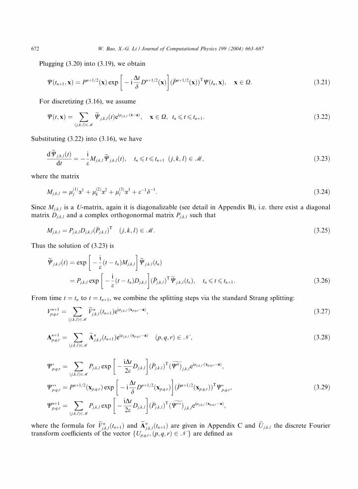
672 W. Bao, X.-G. Li / Journal of Computational Physics 199 (2004) 663–687
Plugging (3.20) into (3.19), we obtain
Wðtnþ1; xÞ ¼ Pnþ1=2ðxÞ exp� i
DtdDnþ1=2ðxÞ
�ð�Pnþ1=2ðxÞÞTWðtn; xÞ; x 2 X: ð3:21Þ
For discretizing (3.16), we assume
Wðt; xÞ ¼X
ðj;k;lÞ2M
eWj;k;lðtÞeilj;k;l�ðx�aÞ; x 2 X; tn 6 t6 tnþ1: ð3:22Þ
Substituting (3.22) into (3.16), we have
d eWj;k;lðtÞdt
¼ � i
eMj;k;l
eWj;k;lðtÞ; tn 6 t6 tnþ1 ðj; k; lÞ 2 M; ð3:23Þ
where the matrix
Mj;k;l ¼ lð1Þj a1 þ lð2Þ
k a2 þ lð3Þl a3 þ e�1d�1: ð3:24Þ
Since Mj;k;l is a U-matrix, again it is diagonalizable (see detail in Appendix B), i.e. there exist a diagonal
matrix Dj;k;l and a complex orthogonormal matrix Pj;k;l such that
Mj;k;l ¼ Pj;k;lDj;k;lð�Pj;k;lÞT ðj; k; lÞ 2 M: ð3:25Þ
Thus the solution of (3.23) is
eWj;k;lðtÞ ¼ exp
� i
eðt � tnÞMj;k;l
� eWj;k;lðtnÞ
¼ Pj;k;l exp� i
eðt � tnÞDj;k;l
�ð�Pj;k;lÞT eWj;k;lðtnÞ; tn 6 t6 tnþ1: ð3:26Þ
From time t ¼ tn to t ¼ tnþ1, we combine the splitting steps via the standard Strang splitting:
V nþ1p;q;r ¼
Xðj;k;lÞ2M
eV nj;k;lðtnþ1Þeilj;k;l�ðxp;q;r�aÞ; ð3:27Þ
Anþ1p;q;r ¼
Xðj;k;lÞ2M
eAnj;k;lðtnþ1Þeilj;k;l�ðxp;q;r�aÞ ðp; q; rÞ 2 N; ð3:28Þ
Wp;q;r ¼
Xðj;k;lÞ2M
Pj;k;l exp� iDt
2eDj;k;l
�ð�Pj;k;lÞT gðWnÞj;k;leilj;k;l�ðxp;q;r�aÞ;
Wp;q;r ¼ Pnþ1=2ðxp;q;rÞ exp
� i
DtdDnþ1=2ðxp;q;rÞ
�ð�Pnþ1=2ðxp;q;rÞÞTW
p;q;r;
Wnþ1p;q;r ¼
Xðj;k;lÞ2M
Pj;k;l exp� iDt
2eDj;k;l
�ð�Pj;k;lÞT gðWÞj;k;leilj;k;l�ðxp;q;r�aÞ;
ð3:29Þ
where the formula for eV nj;k;lðtnþ1Þ and eAn
j;k;lðtnþ1Þ are given in Appendix C and eUj;k;l the discrete Fourier
transform coefficients of the vector fUp;q;r; ðp; q; rÞ 2 Ng are defined as

W. Bao, X.-G. Li / Journal of Computational Physics 199 (2004) 663–687 673
eUj;k;l ¼1
M1M2M3
Xðp;q;rÞ2Q
Up;q;reilj;k;l�ðxp;q;r�aÞ ðj; k; lÞ 2 M; ð3:30Þ
where
Q ¼ ðp; q; rÞ j 0f 6 p6M1 � 1; 06 q6M2 � 1; 06 r6M3 � 1g:
The initial conditions (3.3) and (3.4) are discretized as
W0p;q;r ¼ Wð0Þðxp;q;rÞ; V 0
p;q;r ¼ V ð0Þðxp;q;rÞ;dV 0
p;q;rð0Þdt
¼ V ð1Þðxp;q;rÞ; A0p;q;r ¼ Að0Þðxp;q;rÞ;
dA0p;q;rð0Þdt
¼ Að1Þðxp;q;rÞ; ðp; q; rÞ 2 N:
Remark 3.1. We use the Simpson quadrature rule to approximate the integration in (3.19) instead of the
trapezodial rule which was used in [6,7] for a similar integration. The reason is that we want the quadrature
is exact when the MD system (2.5) and (2.6) admits the plane wave solution (2.23)–(2.25). In this case, theintegrand Gðt; xÞ is quadratic in t. Thus the algorithm (3.27)–(3.29) gives exact results when the MD system
admits plane wave solution.
3.2. Properties of the numerical method
1. Plane wave solution: If the initial data in (3.3) and (3.4) are chosen as in (2.20)–(2.22), and the external
electric and magnetic fields, i.e. V ext and Aext, are chosen as in (2.24) and (2.25), then the MD system (3.1)–
(3.5) admits the plane wave solution (2.23)–(2.25). It is easy to see that in this case our numerical method(3.27)–(3.29) gives exact results provided that Mj P 2ðjxjj þ 1Þ (j ¼ 1; 2; 3).
2. Time transverse invariant: If constants a0 and a1 are added to V ð0Þ and V ð1Þ, respectively, in (3.3), then
the solution V n get added by a0 þ a1tn and Wn get multiplied by e�itnða0þa1tn=2Þ=d, which leaves density of each
particle jwnj j (j ¼ 1; 2; 3; 4) unchanged.
3. Conservation: Let U ¼ fUp;q;r; ðp; q; rÞ 2 Ng and f ðxÞ a periodic function on the box X, and let k � kl2be the usual discrete l2-norm on the box X, i.e.
kUk2l2 ¼ h1h2h3X
ðp;q;rÞ2QjUp;q;rj2; ð3:31Þ
DMeanðUÞ ¼ h1h2h3X
ðp;q;rÞ2QUp;q;r; ð3:32Þ
kf k2l2 ¼ h1h2h3X
ðp;q;rÞ2Qjf ðxp;q;rÞj2: ð3:33Þ
Then we have:
Theorem 3.1. The time splitting spectral method (3.27)–(3.29) for the MD conserves the following quantities in
the discretized level:
kWnkl2 ¼ kW0kl2 ¼ kWð0Þkl2 ; n ¼ 0; 1; 2; . . . ; ð3:34Þ

674 W. Bao, X.-G. Li / Journal of Computational Physics 199 (2004) 663–687
DMeanðV nÞ ¼ DMeanðV ð0ÞÞ þ tnDMeanðV ð1ÞÞ þ t2n2e2
DMeanðjWð0Þj2Þ: ð3:35Þ
Proof. See Appendix D. �
4. Unconditional stability: By the standard Von Neumann analysis for (3.27) and (3.28), noting (3.34), we
get the method (3.27)–(3.29) is unconditionally stable. In fact, setting Wn ¼ 0 and plugging~V nj;k;lðtnþ1Þ ¼ l~V n
j;k;lðtnÞ ¼ l2 ~V n�1j;k;l ðtn�1Þ into (C.3) with jlj the amplification factor, we obtain the characteristic
equation:
l2 � 2l cosðjlj;k;ljDt=eÞ þ 1 ¼ 0; ðj; k; lÞ 2 M: ð3:36Þ
This implies
l ¼ cosðjlj;k;ljDt=eÞ i sinðjlj;k;ljDt=eÞ: ð3:37Þ
Thus the amplification factor
Gj;k;l ¼ jlj ¼ffiffiffiffiffiffiffiffiffiffiffiffiffiffiffiffiffiffiffiffiffiffiffiffiffiffiffiffiffiffiffiffiffiffiffiffiffiffiffiffiffiffiffiffiffiffiffiffiffiffiffiffiffiffiffiffiffiffiffiffiffiffiffiffiffiffiffiffiffifficos2ðjlj;k;ljDt=eÞ þ sin2ðjlj;k;ljDt=eÞ
q¼ 1 ðj; k; lÞ 2 M: ð3:38Þ
Similar results can be obtained for (3.28). These together with (3.34) imply the method (3.27)–(3.29) is
unconditionally stable. This is confirmed by our numerical results in the next section.
5. e-resolution in the ‘nonrelatistic’ limit regime (0 < e � 1): As our numerical results in the next section
suggest: The meshing strategy (or e-resolution) which guarantees ‘good’ numerical results in the ‘nonrel-atistic’ limit regime, i.e. 0 < e � 1, is
h ¼ maxfh1; h2; h3g ¼ OðeÞ; Dt ¼ Oðe2Þ: ð3:39Þ
3.3. For homogeneous Dirichlet boundary conditions
In some cases, the periodic boundary conditions (3.5) may be replaced by the following homogeneous
Dirichlet boundary conditions:
Wðt; xÞ ¼ V ðt; xÞ ¼ 0; Aðt; xÞ ¼ 0; x 2 oX; tP 0: ð3:40Þ
In this case, the method designed above is still valid provided that we replace the Fourier basis functions by
sine basis functions. Let
M ¼ ðj; k; lÞ j 1f 6 j6M1 � 1; 16 k6M2 � 1; 16 l6M3 � 1g;
lð1Þj ¼ pj
b1 � a1; lð2Þ
k ¼ pkb2 � a2
; lð3Þl ¼ pl
b3 � a3ðj; k; lÞ 2 M: ð3:41Þ
W. Bao, X.-G. Li / Journal of Computational Physics 199 (2004) 663–687 675
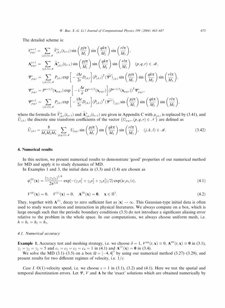
The detailed scheme is:
V nþ1p;q;r ¼
Xðj;k;lÞ2M
eV nj;k;lðtnþ1Þ sin
pjpM1
� �sin
qkpM2
� �sin
rlpM3
� �;
Anþ1p;q;r ¼
Xðj;k;lÞ2M
eAnj;k;lðtnþ1Þ sin
pjpM1
� �sin
qkpM2
� �sin
rlpM3
� �ðp; q; rÞ 2 M;
Wp;q;r ¼
Xðj;k;lÞ2M
Pj;k;l exp� iDt
2eDj;k;l
�ð�Pj;k;lÞT gðWnÞj;k;l sin
pjpM1
� �sin
qkpM2
� �sin
rlpM3
� �;
Wp;q;r ¼ Pnþ1=2ðxp;q;rÞ exp
� i
DtdDnþ1=2ðxp;q;rÞ
�ð�Pnþ1=2ðxp;q;rÞÞTW
p;q;r;
Wnþ1p;q;r ¼
Xðj;k;lÞ2M
Pj;k;l exp� iDt
2eDj;k;l
�ð�Pj;k;lÞT gðWÞj;k;l sin
pjpM1
� �sin
qkpM2
� �sin
rlpM3
� �;
where the formula for eV nj;k;lðtnþ1Þ and eAn
j;k;lðtnþ1Þ are given in Appendix C with lj;k;l is replaced by (3.41), andeUj;k;l the discrete sine transform coefficients of the vector fUp;q;r; ðp; q; rÞ 2 Ng are defined as
eUj;k;l ¼8
M1M2M3
Xðp;q;rÞ2M
Up;q;r sinpjpM1
� �sin
qkpM2
� �sin
rlpM3
� �; ðj; k; lÞ 2 M: ð3:42Þ
4. Numerical results
In this section, we present numerical results to demonstrate ‘good’ properties of our numerical method
for MD and apply it to study dynamics of MD.
In Examples 1 and 3, the initial data in (3.3) and (3.4) are chosen as
wð0Þj ðxÞ ¼ ðc1c2c3Þ
1=4
2p3=4exp½�ðc1x21 þ c2x
22 þ c3x
23Þ=2Þ expðicjx1=eÞ; ð4:1Þ
V ð0ÞðxÞ ¼ 0; V ð1ÞðxÞ ¼ 0; Að0ÞðxÞ ¼ 0; x 2 R3: ð4:2Þ
They, together with Að1Þ, decay to zero sufficient fast as jxj ! 1. This Gaussian-type initial data is often
used to study wave motion and interaction in physical literatures. We always compute on a box, which is
large enough such that the periodic boundary conditions (3.5) do not introduce a significant aliasing error
relative to the problem in the whole space. In our computations, we always choose uniform mesh, i.e.
h ¼ h1 ¼ h2 ¼ h3.
4.1. Numerical accuracy
Example 1. Accuracy test and meshing strategy, i.e. we choose d ¼ 1, V extðt; xÞ � 0, Aextðt; xÞ � 0 in (3.1),c1 ¼ c2 ¼ c3 ¼ 5 and c1 ¼ c2 ¼ c3 ¼ c4 ¼ 1 in (4.1) and Að1ÞðxÞ ¼ 0 in (3.4).
We solve the MD (3.1)–(3.5) on a box X ¼ ½�4; 4�3 by using our numerical method (3.27)–(3.29), and
present results for two different regimes of velocity, i.e. 1=e:
Case I. Oð1Þ-velocity speed, i.e. we choose e ¼ 1 in (3.1), (3.2) and (4.1). Here we test the spatial and
temporal discretization errors. Let W, V and A be the ‘exact’ solutions which are obtained numerically by
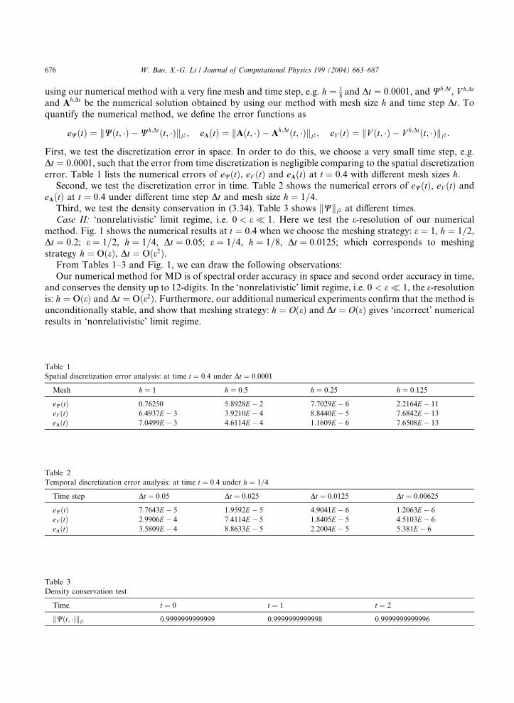
676 W. Bao, X.-G. Li / Journal of Computational Physics 199 (2004) 663–687
using our numerical method with a very fine mesh and time step, e.g. h ¼ 18and Dt ¼ 0:0001, and Wh;Dt, V h;Dt
and Ah;Dt be the numerical solution obtained by using our method with mesh size h and time step Dt. Toquantify the numerical method, we define the error functions as
eWðtÞ ¼ kWðt; �Þ �Wh;Dtðt; �Þkl2 ; eAðtÞ ¼ kAðt; �Þ � Ah;Dtðt; �Þkl2 ; eV ðtÞ ¼ kV ðt; �Þ � V h;Dtðt; �Þkl2 :
First, we test the discretization error in space. In order to do this, we choose a very small time step, e.g.
Dt ¼ 0:0001, such that the error from time discretization is negligible comparing to the spatial discretization
error. Table 1 lists the numerical errors of eWðtÞ, eV ðtÞ and eAðtÞ at t ¼ 0:4 with different mesh sizes h.Second, we test the discretization error in time. Table 2 shows the numerical errors of eWðtÞ, eV ðtÞ and
eAðtÞ at t ¼ 0:4 under different time step Dt and mesh size h ¼ 1=4.Third, we test the density conservation in (3.34). Table 3 shows kWkl2 at different times.
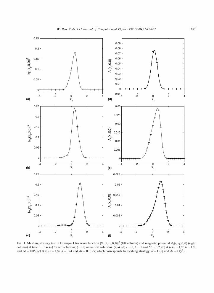
Case II: ‘nonrelativistic’ limit regime, i.e. 0 < e � 1. Here we test the e-resolution of our numerical
method. Fig. 1 shows the numerical results at t ¼ 0:4 when we choose the meshing strategy: e ¼ 1, h ¼ 1=2,Dt ¼ 0:2; e ¼ 1=2, h ¼ 1=4, Dt ¼ 0:05; e ¼ 1=4, h ¼ 1=8, Dt ¼ 0:0125; which corresponds to meshing
strategy h ¼ OðeÞ, Dt ¼ Oðe2Þ.From Tables 1–3 and Fig. 1, we can draw the following observations:
Our numerical method for MD is of spectral order accuracy in space and second order accuracy in time,and conserves the density up to 12-digits. In the ‘nonrelativistic’ limit regime, i.e. 0 < e � 1, the e-resolutionis: h ¼ OðeÞ and Dt ¼ Oðe2Þ. Furthermore, our additional numerical experiments confirm that the method is
unconditionally stable, and show that meshing strategy: h ¼ OðeÞ and Dt ¼ OðeÞ gives ‘incorrect’ numerical
results in ‘nonrelativistic’ limit regime.
Table 1
Spatial discretization error analysis: at time t ¼ 0:4 under Dt ¼ 0:0001
Mesh h ¼ 1 h ¼ 0:5 h ¼ 0:25 h ¼ 0:125
eWðtÞ 0:76250 5:8928E � 2 7:7029E � 6 2:2164E � 11
eV ðtÞ 6:4937E � 3 3:9210E � 4 8:8440E � 5 7:6842E � 13
eAðtÞ 7:0499E � 3 4:6114E � 4 1:1609E � 6 7:6508E � 13
Table 2
Temporal discretization error analysis: at time t ¼ 0:4 under h ¼ 1=4
Time step Dt ¼ 0:05 Dt ¼ 0:025 Dt ¼ 0:0125 Dt ¼ 0:00625
eWðtÞ 7:7643E � 5 1:9592E � 5 4:9041E � 6 1:2063E � 6
eV ðtÞ 2:9906E � 4 7:4114E � 5 1:8405E � 5 4:5103E � 6
eAðtÞ 3:5809E � 4 8:8633E � 5 2:2004E � 5 5:381E � 6
Table 3
Density conservation test
Time t ¼ 0 t ¼ 1 t ¼ 2
kWðt; �Þkl2 0.9999999999999 0.9999999999998 0.9999999999996
(a)–4 –2 0 2 4
0
0.05
0.1
0.15
0.2
0.25
x1
|ψ1(x
1,0,0
)|2
(d)–4 –2 0 2 4
–0.01
0
0.01
0.02
0.03
0.04
0.05
0.06
0.07
0.08
0.09
x1
A 1(x1,0
,0)
(b)–4 –2 0 2 4
0
0.05
0.1
0.15
0.2
0.25
x1
|ψ1(x
1,0,0
)|2
(e)–4 –2 0 2 4
0
0.005
0.01
0.015
0.02
0.025
0.03
x1
A 1(x1,0
,0)
(c)–4 –2 0 2 4
0
0.05
0.1
0.15
0.2
0.25
x1
|ψ1(x
1,0,0
)|2
(f)–4 –2 0 2 4
0
0.005
0.01
0.015
0.02
0.025
x1
A 1(x1,0
,0)
Fig. 1. Meshing strategy test in Example 1 for wave function jW1ðt; x1; 0; 0Þj2 (left column) and magnetic potential A1ðt; x1; 0; 0Þ (rightcolumn) at time t ¼ 0:4. (–) ‘exact’ solutions; (+++) numerical solutions. (a) & (d) e ¼ 1, h ¼ 1 and Dt ¼ 0:2; (b) & (e) e ¼ 1=2, h ¼ 1=2
and Dt ¼ 0:05; (c) & (f) e ¼ 1=4, h ¼ 1=4 and Dt ¼ 0:0125; which corresponds to meshing strategy: h ¼ OðeÞ and Dt ¼ Oðe2Þ.
W. Bao, X.-G. Li / Journal of Computational Physics 199 (2004) 663–687 677
678 W. Bao, X.-G. Li / Journal of Computational Physics 199 (2004) 663–687
4.2. Applications
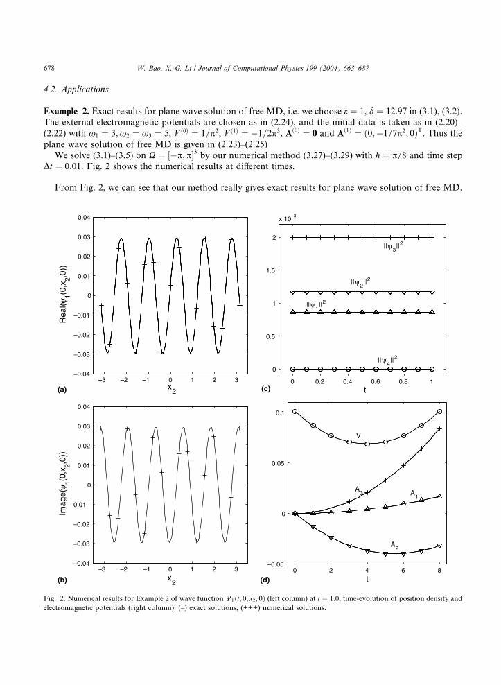
Example 2. Exact results for plane wave solution of free MD, i.e. we choose e ¼ 1, d ¼ 12:97 in (3.1), (3.2).The external electromagnetic potentials are chosen as in (2.24), and the initial data is taken as in (2.20)–
(2.22) with x1 ¼ 3;x2 ¼ x3 ¼ 5, V ð0Þ ¼ 1=p2, V ð1Þ ¼ �1=2p3, Að0Þ ¼ 0 and Að1Þ ¼ ð0;�1=7p2; 0ÞT. Thus theplane wave solution of free MD is given in (2.23)–(2.25)
We solve (3.1)–(3.5) on X ¼ ½�p; p�3 by our numerical method (3.27)–(3.29) with h ¼ p=8 and time step
Dt ¼ 0:01. Fig. 2 shows the numerical results at different times.
From Fig. 2, we can see that our method really gives exact results for plane wave solution of free MD.
(a)–3 –2 –1 0 1 2 3
–0.04
–0.03
–0.02
–0.01
0
0.01
0.02
0.03
0.04
x2
Rea
l(ψ1(0
,x2,0
))
(c)0 0.2 0.4 0.6 0.8 1
0
0.5
1
1.5
2
x 10–3
t
||ψ1||2
||ψ2||2
||ψ3||2
||ψ4||2
(b)–3 –2 –1 0 1 2 3
–0.04
–0.03
–0.02
0.01
0
0.01
0.02
0.03
0.04
x2
Imag
e(ψ
1(0,x
2,0))
(d)0 2 4 6 8
–0.05
0
0.05
0.1
t
A1
A2
A3
V
Fig. 2. Numerical results for Example 2 of wave function W1ðt; 0; x2; 0Þ (left column) at t ¼ 1:0, time-evolution of position density and
electromagnetic potentials (right column). (–) exact solutions; (+++) numerical solutions.
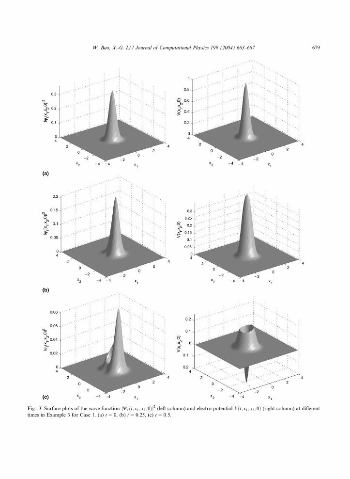
Fig. 3. Surface plots of the wave function jW1ðt; x1; x2; 0Þj2 (left column) and electro potential V ðt; x1; x2; 0Þ (right column) at different
times in Example 3 for Case 1. (a) t ¼ 0, (b) t ¼ 0:25, (c) t ¼ 0:5.
W. Bao, X.-G. Li / Journal of Computational Physics 199 (2004) 663–687 679
(a)0 0.5 1 1.5 2
0.242
0.244
0.246
0.248
0.25
0.252
0.254
0.256
0.258
0.26
||ψ1||2
||ψ2||2
||ψ3||2
||ψ4||2
(b)0 0.5 1 1.5 2
0.05
0.1
0.15
0.2
0.25
0.3
0.35
0.4
0.45
t
||ψ1||2
||ψ2||2
||ψ3||2
||ψ4||2
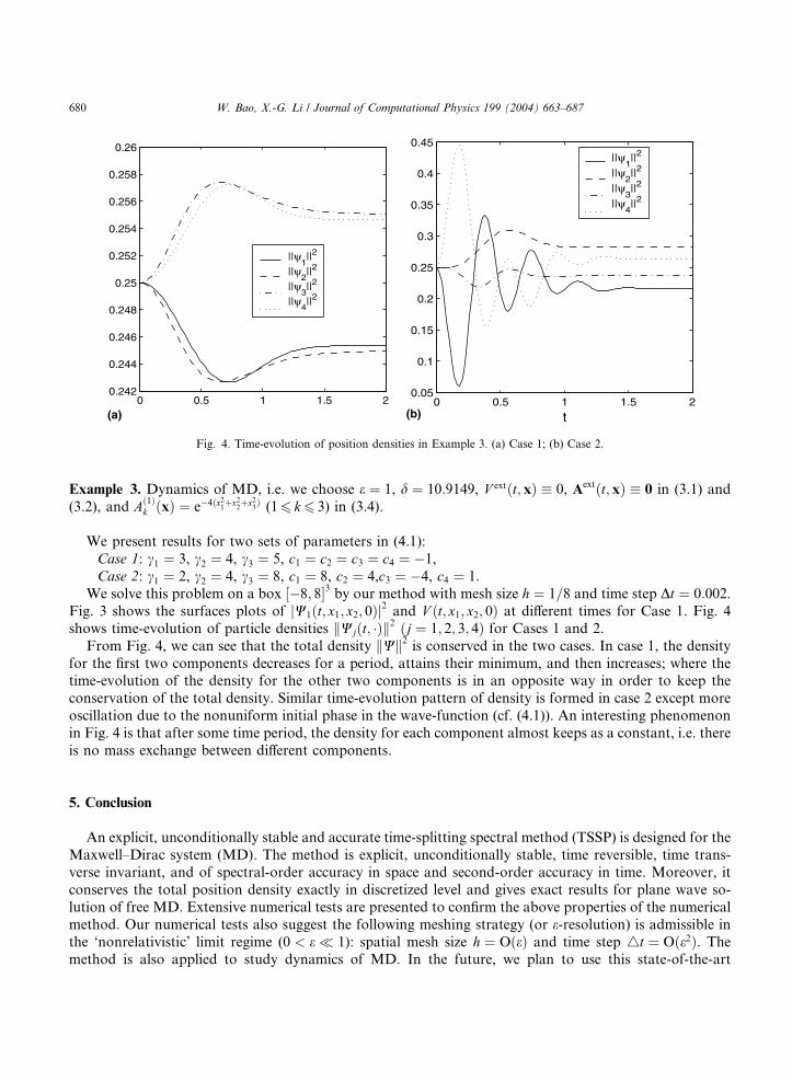
Fig. 4. Time-evolution of position densities in Example 3. (a) Case 1; (b) Case 2.
680 W. Bao, X.-G. Li / Journal of Computational Physics 199 (2004) 663–687
Example 3. Dynamics of MD, i.e. we choose e ¼ 1, d ¼ 10:9149, V extðt; xÞ � 0, Aextðt; xÞ � 0 in (3.1) and
(3.2), and Að1Þk ðxÞ ¼ e�4ðx2
1þx2
2þx2
3Þ (16 k6 3) in (3.4).
We present results for two sets of parameters in (4.1):
Case 1: c1 ¼ 3, c2 ¼ 4, c3 ¼ 5, c1 ¼ c2 ¼ c3 ¼ c4 ¼ �1,
Case 2: c1 ¼ 2, c2 ¼ 4, c3 ¼ 8, c1 ¼ 8, c2 ¼ 4,c3 ¼ �4, c4 ¼ 1.
We solve this problem on a box ½�8; 8�3 by our method with mesh size h ¼ 1=8 and time step Dt ¼ 0:002.Fig. 3 shows the surfaces plots of jW1ðt; x1; x2; 0Þj2 and V ðt; x1; x2; 0Þ at different times for Case 1. Fig. 4
shows time-evolution of particle densities kWjðt; �Þk2 ðj ¼ 1; 2; 3; 4Þ for Cases 1 and 2.
From Fig. 4, we can see that the total density kWk2 is conserved in the two cases. In case 1, the density
for the first two components decreases for a period, attains their minimum, and then increases; where thetime-evolution of the density for the other two components is in an opposite way in order to keep the
conservation of the total density. Similar time-evolution pattern of density is formed in case 2 except more
oscillation due to the nonuniform initial phase in the wave-function (cf. (4.1)). An interesting phenomenon
in Fig. 4 is that after some time period, the density for each component almost keeps as a constant, i.e. there
is no mass exchange between different components.
5. Conclusion
An explicit, unconditionally stable and accurate time-splitting spectral method (TSSP) is designed for the
Maxwell–Dirac system (MD). The method is explicit, unconditionally stable, time reversible, time trans-
verse invariant, and of spectral-order accuracy in space and second-order accuracy in time. Moreover, it
conserves the total position density exactly in discretized level and gives exact results for plane wave so-
lution of free MD. Extensive numerical tests are presented to confirm the above properties of the numerical
method. Our numerical tests also suggest the following meshing strategy (or e-resolution) is admissible in
the ‘nonrelativistic’ limit regime (0 < e � 1): spatial mesh size h ¼ OðeÞ and time step 4t ¼ Oðe2Þ. Themethod is also applied to study dynamics of MD. In the future, we plan to use this state-of-the-art
W. Bao, X.-G. Li / Journal of Computational Physics 199 (2004) 663–687 681
numerical method to study more complicated time-evolution of fast (relativistic) electrons and positrons
within external and self-generated electromagnetic fields.
Acknowledgements
The authors acknowledge support by the National University of Singapore Grant No. R-151-000-027-
112 and thank very helpful discussions with Peter Markowich and Christof Sparber.
Appendix A. Diagnolize the matrix Gnþ1=2(x) in (3.19) and computation
From (3.19), notice (3.18), we have
Gnþ1=2ðxÞ ¼ 1
6Gðtn; xÞ�
þ 4Gðtnþ1=2; xÞ þ Gðtnþ1; xÞ�
¼
V nþ1=2ðxÞ 0 �Anþ1=23 ðxÞ �Anþ1=2
� ðxÞ0 V nþ1=2ðxÞ �Anþ1=2
þ ðxÞ Anþ1=23 ðxÞ
�Anþ1=23 ðxÞ �Anþ1=2
� ðxÞ V nþ1=2ðxÞ 0
�Anþ1=2þ ðxÞ Anþ1=2
3 ðxÞ 0 V nþ1=2ðxÞ
0BBB@1CCCA ðA:1Þ
with
Anþ1=2 ðxÞ ¼ Anþ1=2
1 ðxÞ iAnþ1=22 ðxÞ;
V nþ1=2ðxÞ ¼ 1
6V ðtn; xÞ�
þ V extðtn; xÞ þ 4ðV ðtnþ1=2; xÞ þ V extðtnþ1=2; xÞÞ þ V ðtnþ1; xÞ þ V extðtnþ1; xÞ�;
Anþ1=2ðxÞ ¼ Anþ1=21 ðxÞ;Anþ1=2
2 ðxÞ;Anþ1=23 ðxÞ
� T
; x 2 X;
Anþ1=2k ðxÞ ¼ 1
6Akðtn; xÞ�
þ Aextk ðtn; xÞ þ 4ðAkðtnþ1=2; xÞ
þ Aextk ðtnþ1=2; xÞÞ þ Akðtnþ1; xÞ þ Aext
k ðtnþ1; xÞ�; k ¼ 1; 2; 3:
Since Gnþ1=2ðxÞ is a U -matrix, it is diagonalizable. The characteristic polynomial of Gnþ1=2ðxÞ is
det kI4�
� Gnþ1=2ðxÞ�¼
k� V nþ1=2ðxÞ 0 Anþ1=23 ðxÞ Anþ1=2
� ðxÞ0 k� V nþ1=2ðxÞ Anþ1=2
þ ðxÞ �Anþ1=23 ðxÞ
Anþ1=23 ðxÞ Anþ1=2
� ðxÞ k� V nþ1=2ðxÞ 0
Anþ1=2þ ðxÞ �Anþ1=2
3 ðxÞ 0 k� V nþ1=2ðxÞ
���������
���������¼ k
�h� V nþ1=2ðxÞ
�2 � jAnþ1=2ðxÞj2i2
¼ 0: ðA:2Þ
Thus the eigenvalues of Gnþ1=2ðxÞ are
knþ1=2þ ðxÞ; knþ1=2
þ ðxÞ; knþ1=2� ðxÞ; knþ1=2
� ðxÞ
with

682 W. Bao, X.-G. Li / Journal of Computational Physics 199 (2004) 663–687
knþ1=2 ðxÞ ¼ V nþ1=2ðxÞ jAnþ1=2ðxÞj ¼ V nþ1=2ðxÞ
ffiffiffiffiffiffiffiffiffiffiffiffiffiffiffiffiffiffiffiffiffiffiffiffiffiffiffiffiffiffiffiX3
j¼1
jAnþ1=2j ðxÞj2
vuutand the corresponding eigenvectors are
vnþ1=21 ðxÞ ¼
Anþ1=2� ðxÞ
�Anþ1=23 ðxÞ0
jAnþ1=2ðxÞj
0BBBB@1CCCCA; v
nþ1=22 ðxÞ ¼
Anþ1=23 ðxÞ
Anþ1=2þ ðxÞ
jAnþ1=2ðxÞj0
0BBBB@1CCCCA;
vnþ1=23 ðxÞ ¼
0
�jAnþ1=2ðxÞjAnþ1=2� ðxÞ
�Anþ1=23 ðxÞ
0BBB@1CCCA; v
nþ1=24 ðxÞ ¼
�jAnþ1=2ðxÞj0
Anþ1=23 ðxÞ
Anþ1=2þ ðxÞ
0BBBB@1CCCCA;
Let
Dnþ1=2ðxÞ ¼ diag knþ1=2þ ðxÞ; knþ1=2
þ ðxÞ; knþ1=2� ðxÞ; knþ1=2
� ðxÞ�
;
Pnþ1=2ðxÞ ¼ 1ffiffiffi2
pjAnþ1=2ðxÞj
vnþ1=21 ðxÞ v
nþ1=22 ðxÞ v
nþ1=23 ðxÞ v
nþ1=24 ðxÞ
� :
Thus Dnþ1=2ðxÞ is a diagonal matrix, Pnþ1=2ðxÞ is a complex orthogonormal matrix, and they diagonalize the
matrix Gnþ1=2ðxÞ, i.e.
Gnþ1=2ðxÞ ¼ Pnþ1=2ðxÞDnþ1=2ðxÞð�Pnþ1=2ðxÞÞT; x 2 X: ðA:3Þ
In order to compute Gnþ1=2ðxp;q;rÞ (ðp; q; rÞ 2 M) used in (A.1), we need V ðtn; xp;q;rÞ ¼ V np;q;r, V ðtnþ1; xp;q;rÞ ¼
V nþ1p;q;r , Aðtn; xp;q;rÞ ¼ An
p;q;r, Aðtnþ1; xp;q;rÞ ¼ Anþ1p;q;r, V ðtnþ1=2; xp;q;rÞ and Aðtnþ1=2; xp;q;rÞ. The first four terms are
given in (3.27) and (3.28). The last two terms can be computed as following:
V ðtnþ1=2; xp;q;rÞ ¼X
ðj;k;lÞ2M
eV nj;k;lðtnþ1=2Þ eilj;k;l�ðxp;q;r�aÞ;
Aðtnþ1=2; xp;q;rÞ ¼X
ðj;k;lÞ2M
eAnj;k;lðtnþ1=2Þ eilj;k;l�ðxp;q;r�aÞ;
where for n ¼ 0:
eV 0j;k;lðt1=2Þ ¼
gðV ð0ÞÞj;k;l þ Dt2
gðV ð1ÞÞj;k;l þgðjWð0Þj2Þj;k;lðDtÞ
2=8e2; j ¼ k ¼ l ¼ 0;gðV ð0ÞÞj;k;l �
gðjWð0Þj2Þj;k;l=jlj;k;lj2
�cosðDtjlj;k;lj=2eÞ
þ gðV ð1ÞÞj;k;l sinðDtjlj;k;lj=2eÞ ejlj;k;lj
þ gðjWð0Þj2Þj;k;l=jlj;k;lj2
otherwise:
8>>>>>>><>>>>>>>:
W. Bao, X.-G. Li / Journal of Computational Physics 199 (2004) 663–687 683
eA 0j;k;lðt1=2Þ ¼
gðAð0ÞÞj;k;l þ Dt2
gðAð1ÞÞj;k;l þgðJð0ÞÞj;k;lðDtÞ
2=8e2; j ¼ k ¼ l ¼ 0;
gðAð0ÞÞj;k;l �gðJð0ÞÞj;k;l=jlj;k;lj
2h i
cosðDtjlj;k;lj=2eÞ
þ gðAð1ÞÞj;k;l sinðDjlj;k;lj=2eÞ ejlj;k;lj
þ gðJð0ÞÞj;k;l=jlj;k;lj2
otherwise:
8>>>>>>>><>>>>>>>>:and for n > 0:
eV nj;k;lðtnþ1=2Þ ¼
32eV nj;k;lðtnÞ � 1
2eV n�1j;k;l ðtn�1Þ þ 3
gðjWnj2Þj;k;lðDtÞ2=8e2; j ¼ k ¼ l ¼ 0;
eV nj;k;l �
gðjWnj2Þj;k;l=jlj;k;lj2
�cosðDtjlj;k;lj=2eÞ
þ ð1� cosðjlj;k;ljDt=eÞÞgðjWnj2Þj;k;l=jlj;k;lj
2
� eV n�1
j;k;l ðtn�1Þ þ eV nj;k;lðtnÞ cosðjlj;k;ljDt=eÞ
i� 1
2 cosðjlj;k;ljDt=2eÞþ gðjWnj2Þj;k;l=jlj;k;lj
2otherwise:
8>>>>>>>>>>>>><>>>>>>>>>>>>>:
eA nj;k;lðtnþ1=2Þ ¼
32eAn
j;k;lðtnÞ � 12eAn�1
j;k;lðtn�1Þ þ 3gðJðnÞÞj;k;lðDtÞ
2=8e2; j ¼ k ¼ l ¼ 0;
eAnj;k;l �
gðJðnÞÞj;k;l=jlj;k;lj2
h icosðDtjlj;k;lj=2eÞ
þ ð1� cosðjlj;k;ljDt=eÞÞgðJðnÞÞj;k;l=jlj;k;lj
2h
� eAn�1j;k;lðtn�1Þ þ eAn
j;k;lðtnÞ cosðjlj;k;ljDt=eÞi
� 12 cosðjlj;k;ljDt=2eÞ
þ gðJðnÞÞj;k;l=jlj;k;lj2
otherwise:
8>>>>>>>>>>>><>>>>>>>>>>>>:The discretized current density JðnÞ is computed as
JðnÞp;q;r ¼ ðjðnÞ1 Þp;q;r; ðjðnÞ2 Þp;q;r; ðjðnÞ3 Þp;q;r
� T
;
ðjðnÞk Þp;q;r ¼ hWnp;q;r; a
kWnp;q;ri; k ¼ 1; 2; 3; nP 0 ðp; q; rÞ 2 N:
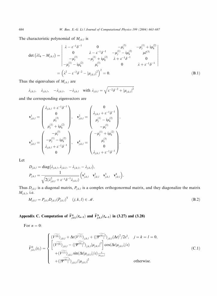
Appendix B. Diagnolize the matrix Mj;k;l in (3.24)
From (3.24), notice (1.7), we have
Mj;k;l ¼ lð1Þj a1 þ lð2Þ
k a2 þ lð3Þl a3 þ e�1d�1 ¼
e�1d�1 0 lð3Þl lð1Þ
j � ilð2Þk
0 e�1d�1 lð1Þj þ ilð2Þ
k �lð3Þl
lð3Þl lð1Þ
j � ilð2Þk �e�1d�1 0
lð1Þj þ ilð2Þ �lð3Þ
0 �e�1d�1
0BBBB@1CCCCA:
k l
684 W. Bao, X.-G. Li / Journal of Computational Physics 199 (2004) 663–687
The characteristic polynomial of Mj;k;l is
det kI4�
�Mj;k;l
�¼
k� e�1d�1 0 �lð3Þl �lð1Þ
j þ ilð2Þk
0 k� e�1d�1 �lð1Þj � ilð2Þ
k llð3Þ
�lð3Þl �lð1Þ
j þ ilð2Þk kþ e�1d�1 0
�lð1Þj � ilð2Þ
k lð3Þl 0 kþ e�1d�1
���������
���������¼ k2
�� e�2d�2 � jlj;k;lj
2 2
¼ 0: ðB:1Þ
Thus the eigenvalues of Mj;k;l are
kj;k;l; kj;k;l; �kj;k;l; �kj;k;l with kj;k;l ¼ffiffiffiffiffiffiffiffiffiffiffiffiffiffiffiffiffiffiffiffiffiffiffiffiffiffiffiffiffiffiffiffie�2d�2 þ jlj;k;lj
2q
and the corresponding eigenvectors are
v1j;k;l ¼
kj;k;l þ e�1d�1
0
lð3Þl
lð1Þj þ ilð2Þ
k
0BBBB@1CCCCA; v2j;k;l ¼
0
kj;k;l þ e�1d�1
lð1Þj � ilð2Þ
k
�lð3Þl
0BBBB@1CCCCA;
v3j;k;l ¼
�lð3Þl
�lð1Þj � ilð2Þ
k
kj;k;l þ e�1d�1
0
0BBBB@1CCCCA; v4j;k;l ¼
�lð1Þj þ ilð2Þ
k
lð3Þl
0
kj;k;l þ e�1d�1
0BBBB@1CCCCA:
Let
Dj;k;l ¼ diag kj;k;l; kj;k;l;�
� kj;k;l;� kj;k;l�;
Pj;k;l ¼1ffiffiffiffiffiffiffiffiffiffiffiffiffiffiffiffiffiffiffiffiffiffiffiffiffiffiffiffiffiffiffiffiffiffiffiffiffiffiffiffiffi
2ðk2j;k;l þ e�1d�1kj;k;lÞq v1j;k;l v2j;k;l v3j;k;l v4j;k;l
� :
Thus Dj;k;l is a diagonal matrix, Pj;k;l is a complex orthogonormal matrix, and they diagonalize the matrix
Mj;k;l, i.e.
Mj;k;l ¼ Pj;k;lDj;k;lð�Pj;k;lÞT ðj; k; lÞ 2 M: ðB:2Þ
Appendix C. Computation of eVnj;k;lðtnþ1Þ and eVn
j;k;lðtnþ1Þ in (3.27) and (3.28)
For n ¼ 0:
eV 0j;k;lðt1Þ ¼
gðV ð0ÞÞj;k;l þ Dt gðV ð1ÞÞj;k;l þgðjWð0Þj2Þj;k;lðDtÞ
2=2e2; j ¼ k ¼ l ¼ 0;gðV ð0ÞÞj;k;l �
gðjWð0Þj2Þj;k;ljlj;k;lj2
�cosðDtjlj;k;lj=eÞ
þ gðV ð1ÞÞj;k;l sinðDtjlj;k;lj=eÞ ejlj;k;lj
þ gðjWð0Þj2Þ =jlj;k;lj2
otherwise:
8>>>>>>><>>>>>>>:ðC:1Þ
j;k;l

W. Bao, X.-G. Li / Journal of Computational Physics 199 (2004) 663–687 685
eA0j;k;lðt1Þ ¼
gðAð0ÞÞj;k;l þ Dt gðAð1ÞÞj;k;l þgðJð0ÞÞj;k;lðDtÞ
2=2e2; j ¼ k ¼ l ¼ 0;gðAð0ÞÞj;k;l �
gðJð0ÞÞj;k;l=jlj;k;lj2
h icosðDtjlj;k;lj=eÞ
þ gðAð1ÞÞj;k;l sinðDtjlj;k;lj=eÞ ejlj;k;lj
þ gðJð0ÞÞj;k;l=jlj;k;lj2
otherwise:
8>>>>>>><>>>>>>>:ðC:2Þ
and for n > 0:
eV nj;k;lðtnþ1Þ ¼
2eV nj;k;lðtnÞ � eV n�1
j;k;l ðtn�1Þ þ gðjWnj2Þj;k;lðDtÞ2=e2; j ¼ k ¼ l ¼ 0;
2 eV nj;k;l �
gðjWnj2Þj;k;l=jlj;k;lj2
�cosðDtjlj;k;lj=eÞ
�eV n�1j;k;l ðtn�1Þ þ 2
gðjWnj2Þj;k;l=jlj;k;lj2
otherwise:
8>>>><>>>>: ðC:3Þ
eAnj;k;lðtnþ1Þ ¼
2eAnj;k;lðtnÞ � eAn�1
j;k;lðtn�1Þ þ gðJðnÞÞj;k;lðDtÞ2=e2; j ¼ k ¼ l ¼ 0;
2 eAnj;k;l �
gðJðnÞÞj;k;l=jlj;k;lj2
h icosðDtjlj;k;lj=eÞ
�eAn�1j;k;lðtn�1Þ þ 2
gðJðnÞÞj;k;l=jlj;k;lj2
otherwise:
8>>><>>>: ðC:4Þ
Appendix D. Proof of Theorem 3.1
Proof. From (3.29), notice (3.30), (3.20) and (3.25), Parseval’s equality, we have
1
h1h2h3kWnþ1k2l2 ¼
Xðp;q;rÞ2Q
Wnþ1p;q;r
��� ���2¼
Xðp;q;rÞ2Q
Xðj;k;lÞ2M
Pj;k;l exp����� � iDt
2eDj;k;l
�ð�Pj;k;lÞT gðWÞj;k;leilj;k;l�ðxp;q;r�aÞ
�����2
¼ M1M2M3
Xðj;k;lÞ2M
Pj;k;l exp���� � iDt
2eDj;k;l
�ð�Pj;k;lÞT gðWÞj;k;l
����2¼ M1M2M3
Xðj;k;lÞ2M
gðWÞj;k;l��� ���2
¼ 1
M1M2M3
Xðj;k;lÞ2M
Xðp;q;rÞ2Q
Wp;q;re
ilj;k;l�ðxp;q;r�aÞ
����������2
¼X
ðp;q;rÞ2QWj j2
¼X
ðp;q;rÞ2QPnþ1=2ðxp;q;rÞ exp
���� � iDtdDnþ1=2ðxp;q;rÞ
�ð�Pnþ1=2ðxp;q;rÞÞTW
p;q;r
����2¼
Xðp;q;rÞ2Q
Wp;q;r
��� ���2 ¼ Xðp;q;rÞ2Q
Wnp;q;r
��� ���2 ¼ 1
h1h2h3kWnk2l2 ; nP 0: ðD:1Þ
Thus the equality (3.34) is obtained by induction.
686 W. Bao, X.-G. Li / Journal of Computational Physics 199 (2004) 663–687
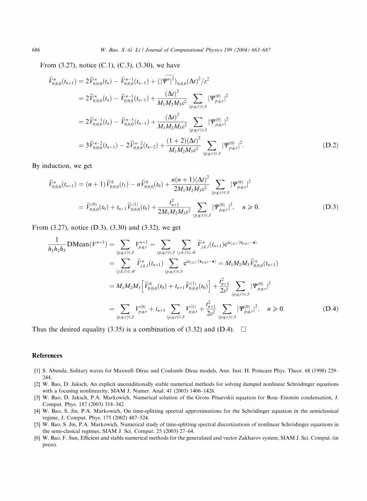
From (3.27), notice (C.1), (C.3), (3.30), we have
eV n0;0;0ðtnþ1Þ ¼ 2eV n
0;0;0ðtnÞ � eV n�10;0;0ðtn�1Þ þ gðjWnj2Þ0;0;0ðDtÞ
2=e2
¼ 2eV n0;0;0ðtnÞ � eV n�1
0;0;0ðtn�1Þ þðDtÞ2
M1M2M3e2X
ðp;q;rÞ2QjWð0Þ
p;q;rj2
¼ 2eV n�10;0;0ðtnÞ � eV n�1
0;0;0ðtn�1Þ þðDtÞ2
M1M2M3e2X
ðp;q;rÞ2QjWð0Þ
p;q;rj2
¼ 3eV n�20;0;0ðtn�1Þ � 2eV n�2
0;0;0ðtn�2Þ þð1þ 2ÞðDtÞ2
M1M2M3e2X
ðp;q;rÞ2QjWð0Þ
p;q;rj2: ðD:2Þ
By induction, we get
eV n0;0;0ðtnþ1Þ ¼ ðnþ 1ÞeV 0
0;0;0ðt1Þ � neV 00;0;0ðt0Þ þ
nðnþ 1ÞðDtÞ2
2M1M2M3e2X
ðp;q;rÞ2QjWð0Þ
p;q;rj2
¼ eV ð0Þ0;0;0ðt0Þ þ tnþ1
eV ð1Þ0;0;0ðt0Þ þ
t2nþ1
2M1M2M3e2X
ðp;q;rÞ2QjWð0Þ
p;q;rj2; nP 0: ðD:3Þ
From (3.27), notice (D.3), (3.30) and (3.32), we get
1
h1h2h3DMeanðV nþ1Þ ¼
Xðp;q;rÞ2Q
V nþ1p;q;r ¼
Xðp;q;rÞ2Q
Xðj;k;lÞ2M
eV nj;k;lðtnþ1Þeilj;k;l�ðxp;q;r�aÞ
¼X
ðj;k;lÞ2M
eV nj;k;lðtnþ1Þ
Xðp;q;rÞ2Q
eilj;k;l�ðxp;q;r�aÞ ¼ M1M2M3eV n0;0;0ðtnþ1Þ
¼ M1M2M3eV 00;0;0ðt0Þ
hþ tnþ1
eV ð1Þ0;0;0ðt0Þ
iþt2nþ1
2e2X
ðp;q;rÞ2QjWð0Þ
p;q;rj2
¼X
ðp;q;rÞ2QV ð0Þp;q;r þ tnþ1
Xðp;q;rÞ2Q
V ð1Þp;q;r þ
t2nþ1
2e2X
ðp;q;rÞ2QjWð0Þ
p;q;rj2; nP 0: ðD:4Þ
Thus the desired equality (3.35) is a combination of (3.32) and (D.4). �
References
[1] S. Abenda, Solitary waves for Maxwell–Dirac and Coulomb–Dirac models, Ann. Inst. H. Poincare Phys. Theor. 68 (1998) 229–
244.
[2] W. Bao, D. Jaksch, An explicit unconditionally stable numerical methods for solving damped nonlinear Schr€odinger equations
with a focusing nonlinearity, SIAM J. Numer. Anal. 41 (2003) 1406–1426.
[3] W. Bao, D. Jaksch, P.A. Markowich, Numerical solution of the Gross–Pitaevskii equation for Bose–Einstein condensation, J.
Comput. Phys. 187 (2003) 318–342.
[4] W. Bao, S. Jin, P.A. Markowich, On time-splitting spectral approximations for the Schr€odinger equation in the semiclassical
regime, J. Comput. Phys. 175 (2002) 487–524.
[5] W. Bao, S. Jin, P.A. Markowich, Numerical study of time-splitting spectral discretizations of nonlinear Schr€odinger equations in
the semi-clasical regimes, SIAM J. Sci. Comput. 25 (2003) 27–64.
[6] W. Bao, F. Sun, Efficient and stable numerical methods for the generalized and vector Zakharov system, SIAM J. Sci. Comput. (in
press).
W. Bao, X.-G. Li / Journal of Computational Physics 199 (2004) 663–687 687
[7] W. Bao, F. Sun, G.W. Wei, Numerical methods for the generalized Zakharov system, J. Comput. Phys. 190 (2003) 201–228.
[8] P. Bechouche, N.J. Mauser, F. Poupaud, (Semi)-nonrelativistic limits of the Dirac equation with external time-dependent
electromagnetic field, Commun. Math. Phys. 197 (1998) 405–425.
[9] J. Bolte, S. Keppeler, A semiclassical approach to the Dirac equation, Ann. Phys. 274 (1999) 125–162.
[10] H.S. Booth, G. Legg, P.D. Jarvis, Algebraic solution for the vector potential in the Dirac equation, J. Phys. A 34 (2001) 5667–
5677.
[11] N. Bournaveas, Local existence for the Maxwell–Dirac equations in three space dimensions, Commun. Partial Differential
Equations 21 (1996) 693–720.
[12] J.M. Chadam, Global solutions of the Cauchy problem for the (classical) coupled Maxwell–Dirac equations in one space
dimension, J. Funct. Anal. 13 (1973) 173–184.
[13] A. Das, General solutions of Maxwell–Dirac equations in 1+1-dimensional space–time and a spatially confined solution, J. Math.
Phys 34 (1993) 3985–3986.
[14] A. Das, An ongoing big bang model in the special relativistic Maxwell–Dirac equations, J. Math. Phys. 37 (1996) 2253–2259.
[15] A. Das, D. Kay, A class of exact plane wave solutions of the Maxwell–Dirac equations, J. Math. Phys. 30 (1989) 2280–2284.
[16] P.A.M. Dirac, Principles of Quantum Mechanics, Oxford University Press, London, 1958.
[17] M. Esteban, E. Sere, An overview on linear and nonlinear Dirac equations, Discrete Contin. Dyn. Syst. 8 (2002) 381–397.
[18] C. Fermanian-Kammerer, Semi-classical analysis of a Dirac equation without adiabatic decoupling, Monatsh. Math. (to appear).
[19] M. Flato, J.C.H. Simon, E. Taflin, Asymptotic completeness, global existence and the infrared problem for the Maxwell–Dirac
equations, Mem. Am. Math. Soc. 127 (1997) 311.
[20] V. Georgiev, Small amplitude solutions of the Maxwell–Dirac equations, Indiana Univ. Math. J. 40 (1991) 845–883.
[21] L. Gross, The Cauchy problem for coupled Maxwell and Dirac equations, Commun. Pure Appl. Math. 19 (1966) 1–15.
[22] W. Hunziker, On the nonrelativistic limit of the Dirac theory, Commun. Math. Phys. 40 (1975) 215–222.
[23] A.G. Lisi, A solitary wave solution of the Maxwell–Dirac equations, J. Phys. A 28 (1995) 5385–5392.
[24] N. Masmoudi, N.J. Mauser, The selfconsistent Pauli equation, Monatsh. Math. 132 (2001) 19–24.
[25] B. Najman, The nonrelativstic limit of the nonlinear Dirac equation, Ann. Inst. Henri Poincare Non Lineaire 9 (1992) 3–12.
[26] C. Sparber, P. Markowich, Semiclassical asymptotics for the Maxwell–Dirac system, J. Math. Phys. 44 (2003) 4555–4572.
[27] H. Spohn, Semiclassical limit of the Dirac equation and spin precession, Ann. Phys. 282 (2000) 420–431.
[28] B. Thaller, The Dirac Equation, Springer, New York, 1992.