An Efficient Convolutional Neural Network for Coronary Heart Disease Prediction

Aniruddha Dutta1, 2, Tamal Batabyal3,6, Meheli Basu4, Scott T. Acton3, 5

1Department of Pathology & Molecular Medicine, Queen’s University, Kingston, ON K7L 3N6, Canada

2Haas School of Business, University of California, Berkeley, CA 94720, USA 3Department of Electrical & Computer Engineering, University of Virginia, VA 22904, USA

4Katz Graduate School of Business, University of Pittsburgh, PA 15260, USA 5Department of Biomedical Engineering, University of Virginia, VA 22904, USA

6Department of Neurology, School of Medicine, University of Virginia, VA 22904, USA

Abstract:

This study proposes an efficient neural network with convolutional layers to classify

significantly class-imbalanced clinical data. The data is curated from the National Health and

Nutritional Examination Survey (NHANES) with the goal of predicting the occurrence of

Coronary Heart Disease (CHD). While the majority of the existing machine learning models that

have been used on this class of data are vulnerable to class imbalance even after the adjustment of

class-specific weights, our simple two-layer CNN exhibits resilience to the imbalance with fair

harmony in class-specific performance. Given a highly imbalanced dataset, it is often challenging

to simultaneously achieve a high class 1 (true CHD prediction rate) accuracy along with a high

class 0 accuracy, as the test data size increases. We adopt a two-step approach: first, we employ

least absolute shrinkage and selection operator (LASSO) based feature weight assessment

followed by majority-voting based identification of important features. Next, the important

features are homogenized by using a fully connected layer, a crucial step before passing the output

of the layer to successive convolutional stages. We also propose a training routine per epoch, akin

to a simulated annealing process, to boost the classification accuracy.

Despite a high class imbalance in the NHANES dataset, the investigation confirms that our

proposed CNN architecture has the classification power of 77% to correctly classify the presence

of CHD and 81.8% to accurately classify the absence of CHD cases on a testing data, which is

85.70% of the total dataset. This result signifies that the proposed architecture can be generalized

to other studies in healthcare with a similar order of features and imbalances. While the recall

values obtained from other machine learning methods, such as SVM and random forest, are

comparable to that of our proposed CNN model, our model predicts the negative (Non-CHD) cases

with higher accuracy. Our model architecture exhibits a way forward to develop better

investigative tools, improved medical treatment and lower diagnostic costs by incorporating a

smart diagnostic system in the healthcare system. The balanced accuracy of our model (79.5%) is

also better than individual accuracies of SVM or random forest classifiers. The CNN classifier

results in high specificity and test accuracy along with high values of recall and area under the

curve (AUC).

Keywords: Coronary heart disease, Machine learning, LASSO regression, Convolutional neural

network, Artificial Intelligence, NHANES

1. Introduction

Heart disease is a leading cause of death today, with coronary heart disease (CHD) being

the most common form of cardiovascular disease that accounts for approximately 13% of deaths

in the US (Benjamin, 2019). Timely diagnosis of heart disease is crucial in reducing health risk

and preventing cardiac arrests. An American Heart Association study projects an almost 100%

increase in CHD cases by 2030 (Benjamin, 2019). Major risk factors such as smoking,

hypertension, hyper cholesterol and diabetes have been studied in connection to CHD (Kannel, et

al., 1971; Stamler, et al., 1993; Vasan, et al., 2001; Kannel, 1996; Burke et al., 1997; Celermajer

et al., 1993; Chobanian et al., 2003; Haskell et al., 1994; Zeiher et al., 1993; Ahmed et al., 2017).

Ahmed. et al. (2017) show that Body Mass Index (BMI) and systolic blood pressure are the two

most critical factors affecting hypertension. Fava. et al. (2013) conclude significant association

between age, sex, BMI and heart rate with hypertension. Studies in general population indicate

that high level of creatinine in blood can increase the risk of CHD (Irie et al., 2006; Wannamethee,

Shaper & Perry 1997). Additionally, blood cholesterol and glycohaemoglobin levels are found to

be persistently and significantly high in patients with CHD (Burchfiel, 1997; Meigs et al., 1997).

Several researchers have used statistical and machine learning models on echocardiography

images (Nakanishi et. al., 2018; Madani et. al., 2018) and electrocardiography signals (Jin, 2009;

Shen et. al., 2016) to predict clinically significant parameters related to CHD in patients, such as

heart rate and axis deviation. Boosted algorithms such as gradient boost and logit boost have been

used in literature to predict FFR and cardiovascular events (Weng et. al, 2017; Goldstein, 2017).

Frizzell et al. and Mortazavi et al. built prediction models to determine the presence of

cardiovascular disease using the 30-day readmission electronic data for patients with heart failure.

The reported C-statistic of the models varied from 0.533 to 0.628, showing an improvement in

prediction with the machine learning approach over traditional statistical methods.

Numerous risk factor variables often make the prediction of CHD difficult, which in turn, increases

the cost of diagnosis and treatment. In order to resolve the complexities and cost of diagnosis,

advanced machine learning models are being widely used by researchers to predict CHD from

clinical data of patients. Kurt et al. (2008) compared prediction performances of a number of

machine learning models including the multilayer perceptron (MLP) and radial basis function

(RBF) to predict the presence of CHD in 1245 subjects (Kurt et al., 2008). The MLP was found to

be the most efficient method, yielding an area under the receiver operating characteristic (ROC)

curve of 0.78. Shilaskar and Ghatol (2013) proposed a hybrid forward selection technique wherein

they were able to select smaller subsets and increase the accuracy of the presence of cardiovascular

disease with reduced number of attributes. Several other groups have reported techniques, such as

artificial neural network (ANN), fuzzy logic (FL) and deep learning (DL) methods to improve

heart disease diagnosis (Uyar, 2017; Venkatesh, 2017). Nonetheless, in most of the previous

studies, the patient cohort was limited to a few thousand with limited risk factors.

We propose an efficient neural network with convolutional layers using the NHANES dataset to

predict the occurrence of CHD. A complete set of clinical, laboratory and examination data are

used in the analysis along with a feature selection technique by LASSO regression. Data

preprocessing is performed using LASSO followed by a feature voting and elimination technique.

The performance of the network is compared to several existing traditional ML models in

conjunction with the identification of a set of important features for CHD. Our architecture is

simple in design, elegant in concept, sophisticated in training schedule, effective in outcome with

far-reaching applicability in problems with unbalanced datasets. Our research contributes to the

existing studies in three primary ways: 1) our model uses a variable elimination technique using

LASSO and feature voting as preprocessing steps; 2) we leverage a shallow neural network with

convolutional layers, which improves CHD prediction rates compared to existing models with

comparable subjects (the ‘shallowness’ is dictated by the scarcity of class-specific data to prevent

overfitting of the network during training); 3) in conjunction with the architecture, we propose a

simulated annealing-like training schedule that is shown to minimize the generalization error

between train and test losses.

It is important to note that our work is not intended to provide a sophisticated architecture using a

neural network. We also do not focus on providing theoretical explanation on how our network

offers resistance to data imbalance. Instead, our goal is to establish that under certain constraints

one can apply convolutional stages despite the scarcity of data and the absence of well-defined

data augmentation techniques and to show that the shallow layers of convolution indeed offer

resilience to the data imbalance problem by dint of a training schedule. The proposed pipeline

contributes to improving CHD prediction rates in imbalanced clinical data, based on a robust

feature selection technique using LASSO and shallow convolutional layers. This serves to improve

prediction algorithms included in smart healthcare devices where sophisticated neural algorithms

can learn from past user data to predict the probability of heart failure and strokes. Prediction rates

could be integrated in healthcare analytics to provide real time monitoring which not only benefits

the patients but also medical practitioners for efficient operations. The present research also

focuses on a systematic training schedule which can be incorporated in smart devices to improve

tracking of different predictor variable levels for heart failure. The rest of the paper is organized

as follows: Section 2 explains data preparation and the preprocessing techniques. In section 3, we

illustrate the convolutional neural network architecture with details on the training and testing

methodology. In section 4 we demonstrate the results obtained from our model with performance

evaluation metrics and compare it with existing models. Section 5 is the conclusion and discussion

section. Here, several extensions to the research are proposed.

2. Data Preprocessing

Our study uses the NHANES data from 1999-2000 to 2015-2016. The dataset is compiled

by combining the demographic, examination, laboratory and questionnaire data of 37,079 (CHD

– 1300, Non-CHD – 35,779) individuals as shown in Figure 1. Demographic variables include age

and gender of the survey participants at the time of screening. Participant weight, height, blood

pressure and body mass index (BMI) from the examination data are also considered as a set of risk

factor variables to study their effect on cardiovascular diseases. NHANES collects laboratory and

survey data from

Figure 1. Data compilation from National Health and Nutritional Survey (NHANES). The data is acquired from 1999

to 2016 in three categories – Demography, Examination and Laboratory. Based on the nature of the factors that are

considered, the dataset contains both the quantitative and the qualitative variables.

Table I: Description of the risk factor independent variables and the dependent variable.

Variable Name Description Code Meaning

Gender Gender of the participant 1

2

Male

Female

Vigorous Activity

12 years and

above

Vigorous activity in last

one week or 30 days

1

2

3

Yes

No

Unable to do activity

Moderate Activity

12 years and

above

Moderate activity in last

one week or 30 days

1

2

3

Yes

No

Unable to do activity

Diabetes

1 yr and above

Doctor told that the

participant has diabetes

1

2

3

Yes

No

Borderline

Blood Relative

Diabetes

20 yrs and above

Biological blood

relatives ever told that

they have diabetes

1

2

Yes

No

Blood Relative

Stroke

20 yrs and above

Biological blood

relatives ever told that

they have hypertension

or stroke before the age

of 50

1

2

Yes

No

Coronary Heart

Disease

20 yrs and above

Ever told that the

participant had coronary

heart disease

1

2

Yes

No

participants once in every two years depending on their age and gender. In addition, based on the

already existing validated experimental research, a comprehensive list of risk factor variables is

selected from the laboratory tests conducted. Questionnaire data comprises of questions asked at

home by interviewers using a Computer-Assisted Personal Interview (CAPI) system as mentioned

in the NHANES website (NHANES, 2015). A total of 5 dichotomous predictor categorical

variables are selected from the questionnaire data which have been shown to affect CHD

(references, required). In all, 30 continuous and 6 categorical independent variables are used to

predict the likelihood of coronary heart disease. For this study, coronary heart disease (CHD) is

used as the dichotomous dependent variable. Awareness of CHD is defined as “yes” response to

the question “Have you been ever told you had coronary heart disease?” Table I shows the

categorical independent and dependent variables in the dataset considered for model development.

The exhaustive list of variables is: gender, age, annual-family-income, ratio-family-income-

poverty, 60sec pulse rate, systolic, diastolic, weight, height, body mass index, white blood cells,

lymphocyte, monocyte, eosinophils, basophils, red blood cells, hemoglobin, mean cell volume,

mean concentration of hemoglobin, platelet count, mean volume of platelets, neutrophils,

hematocrit, red blood cell width, albumin, alkaline phosphatase (ALP), aspartate aminotransferase

(AST), alanine aminotransferase (ALT), cholesterol, creatinine, glucose, gamma-glutamyl

transferase (GGT), cholesterol, creatinine, glucose, iron, iron, lactate dehydrogenase (LDH),

phosphorus, bilirubin, protein, uric acid, triglycerides, total cholesterol, high-density lipoprotein

(HDL), glycohemoglobin, vigorous-work, moderate-work, health-Insurance, diabetes, blood

related diabetes, and blood related stroke. However, in this list of variables, there are a couple of

linearly dependent variables in terms of their nature of acquisition or quantification and some

uncorrelated variables (annual family income, height, ratio of family income-poverty, 60 sec pulse

rate, health insurance, lymphocyte, monocyte, eosinophils, total cholesterol, mean cell volume,

mean concentration of hemoglobin, hematocrit, segmented neutrophils). We do not consider these

variables for subsequent processing and analysis.

3. Proposed Architecture

3.1 LASSO Shrinkage and Majority Voting

LASSO or least absolute shrinkage and selection operator is a regression technique for

variable selection and regularization to enhance the prediction accuracy and interpretability of the

statistical model it produces. In LASSO, data values are shrunk toward a central point, and this

algorithm helps in variable selection and parameter elimination. This type of regression is well-

suited for models with high multicollinearity. LASSO regression adds a penalty equal to the

absolute value of the magnitude of coefficients, and some coefficients can become zero and are

eventually eliminated from the model. This results in variable elimination and hence models with

fewer coefficients. LASSO solutions are quadratic problems and the goal of the algorithm is to

minimize:

∑ (𝑦𝑖 − ∑ 𝑥𝑖𝑗𝛾𝑗

𝑗

)

2

+ 𝜆 ∑ |𝛾𝑗|

𝑝

𝑗=1

(1)

𝑛

𝑖=1

which is the same as minimizing the sum of squares with constraint ∑ |𝛾𝑗| ≤ 𝑠. Some of the 𝛾

values are shrunk to exactly zero, resulting in a regression model that’s easier to interpret. A tuning

parameter, λ which is the amount of shrinkage, controls the strength of the regularization penalty.

When λ = 0, no parameters are eliminated. The estimate is equal to the one found with linear

regression. As λ increases, more coefficients are set to zero and eliminated. As λ increases, bias

increases and as λ decreases, variance increases. The model intercept is usually left unchanged.

The 𝛾 value for a variable (factor) can be interpreted as the importance of the variable in terms of

how the it contributes to the underlying variation in the data. The variable with a zero 𝛾 is

considered unimportant. It is to note that LASSO shows misleading results in case of data

imbalance, which may prompt incorrect selection of important variables if we perform LASSO on

the entire dataset.

Note that the variables in our dataset are mixed data type – a subset of them are categorical. In this

work, as a standard practice, we use group LASSO and we refer it as LASSO for simplicity. In

order to mitigate the effect of imbalance, we adopt a strategy to randomly subsample the dataset

and iterate LASSO multiple times. Majority voting is performed on the set of 𝛾 values to identify

the variable that are nonzero in major number of iterations. Let us assume, that LASSO is

performed N times on N randomly subsampled dataset, where each instance has equal number of

examples in case of CHD and no-CHD. With 45 variables at hand, we obtain 𝛾𝑖 =

[𝛾𝑖,1 𝛾𝑖,2 … … 𝛾𝑖,45 ] at 𝑖𝑡ℎ instance of LASSO. For any variable c, we count the number of

instances in which the variable is non-zero, and with a manually set threshold, we decide the

selection of that variable for further analysis. Mathematically,

𝜒(𝛾) = {1 𝑖𝑓 𝛾 ≠ 00 𝑜𝑡ℎ𝑒𝑟𝑤𝑖𝑠𝑒

[𝜒(𝛾1,𝑐) 𝜒(𝛾2,𝑐) … … 𝜒(𝛾𝑁,𝑐)]𝟏 ≥ 𝑵

𝜶 ⟹ 𝐜 is selected (2)

3.2. Convolutional Neural Network (CNN)

The challenge of predicting the existence of CHD in patients refers to the task of binary

classification. Under certain constraints, neural network (LeCun, 2015; Goodfellow, 2016) has

been proven to be an effective parametric classifier under supervised settings. Recently, with the

explosion of structured data, deep neural networks incorporating a large number of application-

specific hidden layers, have demonstrated significant improvement in several areas including

speech processing, applications involving image processing, and time series prediction (LeCun,

1995). There is a vast body of deep learning architectures that are fine-tuned and rigorously trained

using big datasets. An artificial neural network (Iandola, 2016; Krizhevsky, 2012; Szegedy, 2017;

He, 2016) successively transforms the input data over sequential hidden layers and estimates the

error at the output layer. The error is back propagated to iteratively update the layer weights using

gradient descent algorithm. Rigorous experimentations and analyses have proposed several

improvements in the gradient descent algorithm, the nonlinearity of layers, overfitting reduction,

training schedule, hidden layer visualization and other modifications. Despite resounding success

in applications, the working principle of deep neural networks is still poorly understood. It is also

found in practice that a deep neural network is extremely susceptible to be attacked by adversarial

examples. In addition, owing to millions of parameters in a typical deep architecture, the trained

network may be overfitted, especially in cases where there is scarcity of examples.

Among various algorithms that attempted to overcome this problem, data augmentation

(Krizhevsky, 2012; Radford, 2015) is a widely used technique that artificially generates examples

to populate small datasets. However, such a procedure is biologically implausible in most clinical

datasets. For example, augmented measurements of a CHD phenotype, such as platelet count,

might not correspond to possible readings of a subject. It is because the underlying principles of

the statistical generation and the biological sources of platelet count readings may be

fundamentally different. Poor training due to small or imbalanced datasets and susceptibility to

adversarial examples lead to poor and unreasonable classification. Unlike many computer vision

tasks, such as semantic labeling, chat-bot configuration, and hallucinogenic image synthesis

(Mordvintsev, 2015), erroneous prediction in medical research is accompanied by a significant

penalty.

For example, faulty prediction of a subject having chronic CHD may leave the subject untreated

or misdirect the possible therapeutic medication. Therefore, one of the prime objectives of this

paper is to improve classification accuracy, i.e. the prediction accuracy of the subjects with and

without the presence of CHD. There are several other relevant concerns related to misclassification

in medical research (Marcus, 2018). To overcome these limitations and driven by the success of

deep networks, we propose a shallow convolutional neural network, where the convolution layers

are ‘sandwiched’ between two fully connected layers as shown in Fig. 2.

3.2. CNN Architecture

The architecture is a sequential one-input-one-output feedforward network. For simplicity,

we assume the class of subjects with presence of CHD as class ‘1’ and the subjects with absence

of CHD as class ‘0’. As mentioned in the previous section, the number of active phenotypes of

CHD obtained from majority voting is 50. Let the number of training examples be N, which

Fig 2. Proposed convolutional neural network architecture. The ‘Input’ is a 1D numerical array

corresponding to all the factors/variables from LASSO-Majority Voting preprocessing stage. The ‘Dense’

layer, immediately after the ‘Input’, combines all the factors and each neuron (computing node) at the

output of ‘Dense’ layer is a weighted combination of all the variables, indicating a homogeneous mix of

different variable types. The next two convolution layers seek representation of the input variables via the

‘Dense’ layer. The next two ‘Dense’ layers are followed by the ‘Softmax’ layer. The last two ‘Dense’ layers

(before the ‘Softmax’ layer) can be retrained for transfer learning in case new data is obtained. The

associated training parameters, such as dropout probability, number of neurons, activation function (we

used ReLU), pooling types, and convolution filter parameters are shown in the above figure. Owing to the

large number of parameters that can lead to overfitting of training data points, we propose a training

schedule in section 3.2.1.

indicates that the input layer in Fig. 2 has dimension of ℛ𝑁 𝑋 50. The dense or fully connected

layers, consisting of 64 neurons collectively act as a linear combiner of the 50 variables and bias,

which effectively homogenizes different variable types before nonlinear transformation. The

nonlinear transformation is carried out by rectified linear unit (ReLU). Dropout with 20%

probability is performed to reduce overfitting. Following the fully connected layer, there is a

cascade of convolution layers. In the first convolution layer, there are two filters of kernel width 3

and stride 1. The layer is not provided with external zero-padding. In the pooling layer, we

rigorously experiment with different pooling strategies and find average pooling working

marginally better than max pooling under all constraints. The first convolution layer converts the

output of fully connected block ∈ ℛ𝑁 𝑋 64to a tensor of dimension ℛ𝑁 𝑋 64 𝑋 1. The tensor is then

subjected to batch normalization, nonlinear transformation and average pooling with an output

tensor of dimension ℛ𝑁 𝑋 31 𝑋 2.

The filters in the last no-zero-padded convolution layers are taken with kernel 5 and stride 1,

delivering an output tensor of ℛ𝑁𝑋13𝑋4 to the next dense layer after the average pooling layers.

The categorical output is observed at the end of the softmax layer, where we set the loss function

as the categorical cross-entropy loss. The bias in each layer is initialized with random numbers

drawn from a truncated normal distribution with variance 1

√𝑛, where 𝑛 is the number of ‘fan-in’

connections to the layer. We use Adam optimizer with learning rate 0.005, 𝛽1 = 0.9, 𝛽2 = 0.999

and zero decay. Our proposed architecture consists of 32,642 trainable and 1,164 non-trainable

parameters. We experiment with several hyperparameters that are associated with our model to

obtain consistent class-wise accuracy. We provide results by varying subsampling of input data,

epochs, class-weights, the number of neurons in each dense layer except the last one, and the

number of filters in each convolution layer during training.

3.2.1. Training schedule

During training, the class weight ratio, which is adjusted as a penalty factor due to class

imbalance, is defined as the ratio of CHD and Non-CHD dataset. For example, a class weight ratio

of 10:1 indicates that any misclassification of a CHD training sample will be penalized 10 times

more than a misclassified Non-CHD sample during the error calculation at the output prior to

backpropagation after each epoch. Although, we use dropout layers in our CNN model, we also

use this training schedule in order to further reduce possible overfitting. The intuition is to initially

train the model with 1:Ν weight ratio for sufficiently large number of epochs and then, gradually

increase the weight ratio with a steady decline in the number of epochs. Let the actual class weight

ratio is 𝜌0: 1, which we take as a factor 𝜌0.

Fitting our CNN model, M, by varying the number of epochs (𝜔) and weight ratio (𝜌)

1. Initialize 𝜌 = Ν, 𝜔 (large number, we set as Ν), M, end_iter (5-10 depending on the instance), i=1

2. While 𝜌 ≤ 𝜌0

M.fit (Data, 𝜔, 𝜌)

𝜌 ← 𝑓𝑙𝑜𝑜𝑟(𝜌

2)

𝜔 ← 𝑓𝑙𝑜𝑜𝑟 (𝜔

2)

3. While (𝑖 ≤ 𝑒𝑛𝑑_𝑖𝑡𝑒𝑟) and 𝑇𝑟𝑎𝑖𝑛𝑙𝑜𝑠𝑠(𝑖) ≤ 𝑇𝑟𝑎𝑖𝑛𝑙𝑜𝑠𝑠(𝑖 − 1)

M.fit (Data, 𝑖, 𝜌0)

3.3 Competitive Approaches

Machine learning classification methods have shown to potentially improve prediction

outcomes in coronary heart disease. Such classification methods include logistic regression,

support vector machines, random forests, boosting methods and multilayer perceptron (Goldstein,

2017). Logistic regression models the prediction of a binomial outcome with one or more

explanatory variables, using a standard logistic function which measures the relationship between

the categorical dependent variable and one or more independent variables by estimating the

probabilities. The logistic function is given by, 𝑓(𝑥) =1

1+𝑒−𝑥 which in common practice is known

as the sigmoid curve. Support vector machine (SVM) is a binary classification algorithm which

generates a (N-1) dimensional hyperplane to separate points into two distinct classes in an N

dimensional plane. The classification hyperplane is constructed in a high dimensional space that

represents the largest separation, or margin, between the two classes.

Random forests are an ensemble learning algorithm where decision trees that grow deep are

averaged and trained on different parts of the training set to reduce variance and avoid overfitting.

Random forests algorithm employs bagging or bootstrap aggregating and at each split a random

subset of features are selected. Bagging is a parallel ensemble because each model is built

independently. Boosting on the other hand is a sequential ensemble where each model is built

based on correcting the misclassifications of the previous model. In boosting methods, the weights

are initialized on training samples and for n iterations, a classifier is trained using a single feature

and training error evaluated. Then the classifier with the lowest error is chosen and the weights are

updated accordingly; the final classifier is formed as a linear combination of n classifiers. A boost

classifier is in the form, 𝐹𝑇(𝑥) = ∑ 𝑓𝑡(𝑥)𝑇𝑡=1 where each 𝑓𝑡 is a weak learner with 𝑥 as input. Each

weak learner produces an output hypothesis, h(xi), for each sample in the training set. At each

iteration t, a weak learner is selected and assigned a coefficient 𝛼𝑡 such that the sum training error

Et of the resulting t-stage boost classifier is minimized. A multilayer perceptron (MLP) is a

feedforward artificial neural network (ANN) which consists of an input layer, an output layer and

one or more hidden layers and utilizes backpropagation for training the data. The MLP commonly

uses a nonlinear activation function which maps the weighted inputs to the output of each neurons

in the hidden layers. In an MLP, the connection weights are changed based on the error between

the generated output and expected result. Two of the most common activation functions are the

rectified linear unit (ReLU), 𝑓(𝑥) = 𝑥+ and the hyperbolic tangent, 𝑦(𝑥𝑖) = tanh (𝑥𝑖).

Data augmentation demands attention in the context of data imbalance. Algorithms, such as

random oversampling (ROS), synthetic minority over-sampling technique (SMOTE) (Chawla,

2002), and adaptive synthetic sampling (ADASYN) (He, 2008) augment the minority class data

by either replicating or synthesizing new data. One pertinent issue with regard to synthesized data

is that, unlike images, the data in the context of biological factors (variables) may be implausible

as it is difficult to verify the authenticity of newly augmented data, especially when both classes

of data are closely spaced. In this paper, we provide comparative results by using the above

algorithms. In addition, we provide the corresponding visualization of the augmented data via t-

SNE. Please keep in mind that t-SNE is a non-convex algorithm, generating embedding that

depends on the initialization low-dimensional embedding. We employ random undersampling

strategy to select a subset of data for training the CNN. Similar to data augmentation, there are

several data undersampling strategies. We compare our results with edited nearest neighbor (EDN)

(Wilson, 1972), instance hardness threshold (IHT) (Smith et al., 2014) and three versions of near-

miss (NM-v1, v2 and v3) (Mani, 2003) algorithms.

4 Results

4.1 Summary Statistics

For the purpose of variable selection in our classification model, we start out by

investigating correlations among 30 continuous predictor variables. Correlation is found to be high

(0.77) between serum alanine aminotransferase (ALT) and aspartate aminotransferase (AST) as

given from Fig 3. However, AST is a major risk factor in the prediction of CHD, as has been

reported in the literature (Shen et. al, 2015). Jianying (2015) finds AST levels to be significantly

higher in CHD patients than in the control group and hence can be used as biochemical markers to

predict the severity of CHD. A high correlation of 0.89 was determined between body-mass-index

and weight which seemed normal whereas correlation between hemoglobin and red blood cells

was 0.74. While the association of hemoglobin with clinically recognized CHD is limited in

research (Chonchol, 2008), the role of red blood cells in CHD is well researched in the literature

(Madjid, 2013). It has been investigated that high blood glucose levels for non-diabetic patients

can significantly increase the risk for development of CHD (Neilson, 2006) which is depicted in

Fig. 3 by a high correlation value of 0.79 between glycohemoglobin and glucose. Further, we find

a correlation of 0.46 between protein and albumin. Lower levels of serum albumin have been

reported to be linked with increased levels of cardiovascular mortality as well as CHD (Shaper,

2004) while higher level of protein is reported to increase risks of CHD (Clifton, 2011). Serum

Lactate dehydrogenase (LDH) is found to be correlated with AST (correlation coefficient of 0.41),

consistent with previous studies which suggest that increased value of LDH in active population

is associated with low risk of CHD (Kopel et. al., 2012). Due to the importance of the risk factors

(as reported in existing literature) of some of the correlated variables and their association with

Fig. 3. Correlation table for the independent predictor variables. In this table, moderately strong correlations

among few pairs are observed (Glucose and Glycohemoglobin, Red blood cells and Hemoglobin, ALT and

AST, Weight and Body-Mass-Index). Rest of the pairs show fairly low correlation values, implying the

variables after the LASSO-Majority voting stage are sufficiently decorrelated.

CHD, LASSO regression was performed to correctly determine the predictor variables for further

analysis.

4.2 Model results

To identify variables that contribute to the variation in data, we apply LASSO to 100

instances of randomly sampled datasets, with each containing 1300 examples of class CHD

(negative class) and 1300 of class no-CHD (positive class). We set 𝛼 in eq. (2) as 6 and find that

ALT, glucose, hemoglobin, body mass index fails to contribute significantly in the data

irrespective of strong experimental evidence in state-of-the-arts that favor those factors. From

majority voting, some of the strong correlates are age, white blood cells, platelet count, red cell

distribution width, cholesterol, LDH, uric acid, triglycerides, HDL, glycohemoglobin, gender,

presence of diabetes, blood related stroke, moderate and vigorous work.

Fig. 4. Model accuracy as a function of majority voting threshold. The threshold value of majority voting

affects the classification accuracy of CHD as the selection of this value controls the number of variables

that are to be channeled to our CNN model. The smaller is the threshold value, the larger is the set of

variables. Based on the training loss, training accuracy and test accuracy, the threshold value between 16.67

(100/6) – 20 (100/5) combining 100 instances of LASSO appears suitable for obtaining balanced per class

(CHD and Non-CHD) classification accuracy.

To achieve the optimal number of features for training our CNN architecture, the threshold of the

feature voting was kept in the range of 2 to 8. The highest accuracy obtained from training the

network is 83.17% with a training loss of 0.489 with a threshold feature of 6 as shown in Fig. 4.

The corresponding highest test accuracy obtained is 82.32%. LASSO regularization reduces the

coefficients of three of the continuous predictor variables (Body-mass-index, glucose and ALT)

and one categorical variable to zero which is determined to be highly correlated as seen in section

4.1. With a threshold value of 6, the CNN architecture is trained separately on different sets of

subsampled data sets. Subsampling is performed in varying ratios starting with the range

1300:13000 (CHD: Non-CHD) and increased to 1300:4000 as shown in Table II. The corresponding

test accuracy is reported as 82.32%.

Table II: Training schedule for increasing class weight ratio and sampling for optimal threshold. A

maximum training accuracy if 83.51% and minimum training loss of 0.489 is achieved with a

misclassification penalty of 3:1 (CHD: Non-CHD) and a sampling ratio of 1300:4000 (CHD: Non-CHD).

In each subsampled set, all CHD subjects are taken into consideration and the Non-CHD subjects

are randomly chosen without replacement. For training purposes, the neural network is trained by

varying the misclassification penalty from 10:1 (CHD: Non-CHD) to 3:1 as shown in Table II.

The maximum accuracy of 83.51% and minimum training loss of 0.489 is obtained while training

with a sampling ratio of 1300:4000 (CHD: Non-CHD) and misclassification penalty of 3:1(CHD:

Non-CHD). The trained network is tested on a cohort of 31,779 (85.70% of the whole dataset)

remaining samples and a test accuracy of 82.32% is obtained subsequently as reported in table II.

The optimal sampling ratio (1300:4000) of class 1 to class 0 is maintained for the final training of

the network as illustrated in Table III.

Table III reports the final training of the CNN architecture with varying class (CHD: Non-CHD)

weights to check for consistency of our results. With decrease in class weights, the training

accuracy increases from 59.43% to 83.17% when the difference between the training and test

accuracies becomes a minimum, indicating a reasonable generalization error as shown in Fig. 5.

During training the number of epochs, the number of neurons in each dense layer except the last

one, and the number of filters in each convolution layer are varied to obtain the best fit of the

model. We have fine-tuned several hyperparameters that are associated with our model to obtain

consistent class-wise accuracy. The optimization is performed using Adam as the activation

function with a learning rate 0.006 and 60 epochs, and no scheduling of learning rate is used during

the training. The best test accuracy obtained is 82.32% where the penalty of misclassification of

class 1 is set three times higher than that of class 0.

Class Weight Sampling TPR TNR Train Accuracy (%) Test Accuracy (%) Training Loss

10:1

8:1

6:1

5:1

3:1

1300:13000

1300:10000

1300:8000

1300:6000

1300:4000

0.690

0.706

0.741

0.735

0.778

0.812

0.827

0.799

0.80

0.823

78.00

77.28

80.00

80.48

83.51

81.09

82.67

79.90

79.96

82.32

0.684

0.676

0.595

0.548

0.489

Table III: Training schedule for increasing class weight ratio and optimal sampling ratio attained from table

I. The difference between the training (83.17%) and test (82.32%) accuracies attain the minimum when the

misclassification penalty of class 1 is set three times higher than class 0.

Fig. 5. Training and test accuracies with varying misclassification penalties for class 1 and 0. The minimum

difference between training and test accuracies is obtained with a class weight of 3:1 (CHD: Non-CHD)

and a training loss = 0.489. The model is trained with a constant optimized learning rate of 0.006 and 60

epochs.

The performance of the proposed CNN classifier can be evaluated from the confusion matrix in

Table IV. We specify the classification parameters as follows:

TP: true positive classification cases (true predictions for class 1, i.e., true CHD predictions),

TN: true negative classification cases (true predictions for class 0, i.e., true non- CHD predictions),

Class Weight TPR TNR Train Accuracy (%) Test Accuracy (%) Training Loss

50:1

25:1

12:1

8:1

6:1

4:1

3:1

0.980

0.923

0.860

0.836

0.817

0.788

0.773

0.383

0.568

0.664

0.686

0.740

0.770

0.818

59.43

67.06

71.98

75.08

80.13

81.00

83.17

44.48

58.04

66.60

69.76

74.12

77.10

82.32

1.591

1.236

0.965

0.765

0.620

0.550

0.489

FN: false negative classification cases (false predictions for class 1, i.e., false CHD predictions),

FP: false positive classification cases (false predictions for class 0, i.e., false non- CHD

predictions).

Some commonly applied performance rates calculated are the true positive rate (TPR), the

accuracy of predicting CHD (class 1) and the true negative rate (TNR), the accuracy of predicting

non-CHD (class 0). The detailed values of TPR, TNR, train accuracy, test accuracy and training

loss for all class weights are given in Table III.

Table IV: Confusion matrix for the CNN classifier for coronary heart disease. Out of 208 coronary heart

disease cases in the sample cohort, 161 cases were predicted correctly by the classifier. The proposed

classifier also correctly predicts 25,828 cases where patient did not report coronary heart disease.

In the present study, it is our objective for our classifier to predict the presence of CHD with higher

(improved) accuracy than in previous studies. The recall rate (sensitivity) for correctly predicting

the true positive rate for class 1 (presence of CHD) is 77% while the class 0 (absence of CHD) is

81%. The CNN classifier has been tested on 31,779 subjects while maintaining almost the same

TPR and TNR, contrary to previous reported studies which have considered significantly smaller

samples.

Partitioning a highly imbalanced dataset poses a lot of challenges and incurs unavoidable biases

on a classifier’s performance. While, it is advised to keep same ratio of class-specific data in

training and testing in state of the arts, however, in a highly imbalanced dataset it is often very

challenging to get a high class 1 (true CHD prediction rate) accuracy as the testing data size

increases. The present method confirms that our proposed CNN architecture has the classification

power of 77% to correctly classify the presence of CHD cases on a testing data, which is 85.70%

of the total dataset. This result signifies that the proposed architecture can be generalized to other

studies in healthcare with a similar order of features and imbalances.

The performance of our binary classifier is calculated by computing the ROC curve (Yang et. al;

2017). The area under the curve (AUC) value in the ROC curve is the probability that our proposed

CNN classifier ranks a randomly chosen positive case (CHD) higher than a randomly chosen

negative case (Non-CHD) (Tom 2005). Thus, the ROC curve behaves as a tool to select the

possible optimal models and to reject the suboptimal ones, independently from the class

distribution. It does so by plotting parametrically the true positive rate (TPR) vs the false positive

rate (FPR) at various threshold settings as shown in Fig. 4. (Right). The calculated AUC is 0.767

or 76.7% which is comparable to previous studies related to CHD (Martinez, Schwarcz, Valdez &

Diaz, 2018). In highly imbalanced data sets balanced accuracy is often considered to be a more

accurate metric than normal accuracy itself. The balanced accuracy of the model is determined to

be (TPR + TNR)/2 = 0.795 or 79.5%. The fall out rate or the Type-I error of the model is

5743/31571 = 18.2% and the miss rate or the Type-II error of the model is 47/210 = 22.6%. The

positive likelihood ratio of the predicted model is 4.27 indicating that there is almost a 30%

increase in probability post diagnosis in prediction of the presence of CHD in patients. A negative

likelihood ratio of 0.27 was calculated which signifies that there is approximately 30% decrease

in probability post diagnosis in prediction of absence of CHD in patients.

4.3. Comparison of ML models

4.3.1. Comparison with state-of-the-art ML models

Machine learning models discussed in section 3.3 are implemented and tested on our test cohort.

The prediction results from these methods are then compared with the results of our proposed CNN

architecture. All models are implemented with optimized parameters and then compared based on

the true positive rate (recall) and true negative rate (sensitivity). Corresponding test accuracies and

AUC values are also determined. Logistic regression and adaboost classification result in highest

test accuracies but these classifiers suffer from low recall values which is the true positive rate for

coronary heart disease detection. While the recall values obtained from SVM and random forest

are comparable to that of our proposed CNN model, our model predicts the negative (Non-CHD)

cases with higher accuracy as shown in Table V. The balanced accuracy of our model (79.5%) is

also higher than individual accuracies from that of SVM or random forest classifiers. An optimized

two-layer multilayer perceptron resulted in a low recall value of 66.34% when tested on our test

cohort. Results in Table V show that SVM and random forest classifiers perform better than

logistic, adaboost and MLP classifiers, but the specificity and test accuracy are significantly lower

as compared to our designed CNN classifier. The CNN classifier results in high specificity and

test accuracy along with high values of recall and AUC.

Table V: Comparison of machine learning models for coronary heart disease prediction. As compared to

traditional machine learning models, our proposed model attains a recall value of 0.77 which is comparable

to the SVM classifier. However, specificity (0.81) and test accuracy (0.82) of our model are significantly

higher than the SVM classifier.

Recall (%) Specificity (%) Test Accuracy (%) AUC

Logistic Regression 51.44 91.15 90.89 71.29

SVM 77.40 77.87 77.87 77.64

Random Forest 76.44 76.06 76.06 76.25

AdaBoost 52.88 90.36 90.12 71.63

MLP 66.34 78.88 78.80 72.61

Our model 77.3 81.8 81.78 76.78

These results confirm that the CNN classifier outperforms all existing commonly used machine

learning models for coronary heart disease prediction in terms of accuracy in prediction for both

CHD and Non-CHD classes.

4.3.2. Our LASSO-CNN vs vanilla CNN

Our experimental set up is generalized in the sense that setting 𝑁

𝛼 as 0 (or, equivalently 𝛼 = ∞)

will select all the variables into consideration. Thus, applying vanilla CNN is equivalent to

applying the model LASSO (∞) - CNN. Using the same subsampled dataset with 3:1 ratio of class

samples, vanilla CNN yields 79.42% test accuracy, which is approximately 2% less than the

average test accuracy that we obtain on an average by applying LASSO (6)-CNN. Although, it

seems a marginal improvement, the number of samples in excess that are accurately labeled by our

model is 635 (≈31779*0.02).

4.3.3. Data oversampling strategies

Fig. 6. Results using three oversampling techniques for the data augmentation of the minority class. For

each technique, the results provide training accuracy, test accuracy, training loss, CHD accuracy (class-

specific) and no-CHD accuracy (class-specific) over a number of epochs, added with t-SNE low-

(a)

(d)

(e) (f)

(b)

(c)

dimensional embedding for data visualization in 3D. (a) t-SNE visualization of 90% of the original data

used for training. 10% of the data is reserved for testing. (b) The results using random oversampling (ROS).

Note that we did not provide the t-SNE visualization for ROS as, in ROS, data samples from the minority

class are randomly picked and added to the data, thereby maintaining the same data with redundant samples.

So, the visualization is same as the original data in (a). (c)-(d) Results using SMOTE with visualization.

(e)-(f) Results using ADASYN with visualization.

We compare our LASSO-CNN with the state-of-the-art oversampling algorithms. Note that the

size of the testing dataset is remarkably small in oversampling cases, where the minority class is

oversampled to become cardinally same with the majority class. In case of ROS and SMOTE, each

class of the training data contains 32013 samples and the test data has 3709 samples (CHD: 3558

samples, no-CHD: 151 samples). In case of ADASYN, the training data size is 64134 (CHD:

32121 samples, no-CHD: 32013 samples) and the test data size is identical to ROS.

In all the cases, the ratio of class-specific samples (no-CHD:CHD) in the test data is approximately

24:1. From Fig. 6, it can be seen that, in all the three algorithms, the test accuracy of the no-CHD

class strongly follows the overall test accuracy, indicating the predominant effect of data

imbalance in the test data. Except in ADASYN, it is observed that the test accuracy increases with

our model being trained using more epochs. The increase in the test accuracy is favored by the

increase in the no-CHD accuracy at the expense of compromising CHD accuracy.

Overall, the behavior of LASSO+CNN using SMOTE is erratic, whereas trends in train accuracy,

test accuracy, train loss can be clearly observed in cases of ROS and ADASYN. Although, the test

accuracy is higher in case of SMOTE when compared with ROS and ADASYN, the class-specific

accuracies are balanced in case of ADASYN, yielding 79%, 79.14% and 75.5% for test accuracy,

no-CHD accuracy and CHD accuracy respectively, with the class score variance of 3.06. In terms

of class score variance, ROS trails behind ADASYN, scoring 78.67%, 80% and 74% with 9 as the

class score variance. Class score variance measures how close the CHD and no-CHD accuracies

are.

4.3.4. Data undersampling strategies

We train and test our LASSO+CNN model on several datasets that are undersampled by NM (v1,

v2 and v3), IHT and EDN, as discussed in section 3.3. In case of undersampled datasets, the size

of the test dataset is large as the size of the majority class (no-CHD) is reduced against the minority

class (CHD). After applying an undersampling technique, the samples that are not considered in

(e) (f)

(a) (b)

(c) (d)

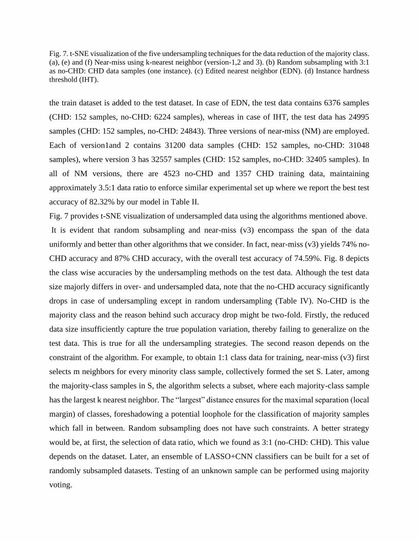
Fig. 7. t-SNE visualization of the five undersampling techniques for the data reduction of the majority class.

(a), (e) and (f) Near-miss using k-nearest neighbor (version-1,2 and 3). (b) Random subsampling with 3:1

as no-CHD: CHD data samples (one instance). (c) Edited nearest neighbor (EDN). (d) Instance hardness

threshold (IHT).

the train dataset is added to the test dataset. In case of EDN, the test data contains 6376 samples

(CHD: 152 samples, no-CHD: 6224 samples), whereas in case of IHT, the test data has 24995

samples (CHD: 152 samples, no-CHD: 24843). Three versions of near-miss (NM) are employed.

Each of version1and 2 contains 31200 data samples (CHD: 152 samples, no-CHD: 31048

samples), where version 3 has 32557 samples (CHD: 152 samples, no-CHD: 32405 samples). In

all of NM versions, there are 4523 no-CHD and 1357 CHD training data, maintaining

approximately 3.5:1 data ratio to enforce similar experimental set up where we report the best test

accuracy of 82.32% by our model in Table II.

Fig. 7 provides t-SNE visualization of undersampled data using the algorithms mentioned above.

It is evident that random subsampling and near-miss (v3) encompass the span of the data

uniformly and better than other algorithms that we consider. In fact, near-miss (v3) yields 74% no-

CHD accuracy and 87% CHD accuracy, with the overall test accuracy of 74.59%. Fig. 8 depicts

the class wise accuracies by the undersampling methods on the test data. Although the test data

size majorly differs in over- and undersampled data, note that the no-CHD accuracy significantly

drops in case of undersampling except in random undersampling (Table IV). No-CHD is the

majority class and the reason behind such accuracy drop might be two-fold. Firstly, the reduced

data size insufficiently capture the true population variation, thereby failing to generalize on the

test data. This is true for all the undersampling strategies. The second reason depends on the

constraint of the algorithm. For example, to obtain 1:1 class data for training, near-miss (v3) first

selects m neighbors for every minority class sample, collectively formed the set S. Later, among

the majority-class samples in S, the algorithm selects a subset, where each majority-class sample

has the largest k nearest neighbor. The “largest” distance ensures for the maximal separation (local

margin) of classes, foreshadowing a potential loophole for the classification of majority samples

which fall in between. Random subsampling does not have such constraints. A better strategy

would be, at first, the selection of data ratio, which we found as 3:1 (no-CHD: CHD). This value

depends on the dataset. Later, an ensemble of LASSO+CNN classifiers can be built for a set of

randomly subsampled datasets. Testing of an unknown sample can be performed using majority

voting.

Fig. 8. Results using the undersampling algorithms from fig. 6 (a)-(e). (a) CHD detection accuracies over

epochs using the algorithms. (b) Detection accuracies of no-CHD test data. Among all the competitive

undersampling strategies that we compare our results with, near-miss (version 3) works better in improving

both class-specific accuracies.

(b)

(a)

(b)

4.4. Validation on stroke data

It might appear that sequentially arranged, multiple convolutional layers in our proposed model

offer resistance to data imbalance only for the CHD data provided by NHANES. To check whether

our model is resilient to other imbalanced datasets containing 1D measurement variables, we apply

our network on a similar dataset on Stroke, which is also compiled by NHANES. The Stroke

dataset contains 37177 subjects and 36 mixed-type measurement variables. Out of 37177 subjects,

there are 1269 subjects who reported that they had strokes. After applying LASSO, we found 34

variables which are important for further processing.

Table VI: Comparison of machine learning models for stroke prediction.

CHD acc (%) No-CHD acc (%) Test Accuracy (%)

Logistic Regression 74 76.8 76.79

SVM 75 74.75 74.74

Random Forest 74 74.45 74.44

AdaBoost 40 90.1 90

Vanilla-CNN 71 77.04 77.01

Our model 74 79.86 79.85

All the models are trained with data from 1169 patients having CHD and 4300 without CHD. Except our

model, we do not apply LASSO prior to training the models. While random forest and SVM yield smaller

differences in accuracies between CHD and No-CHD, they fall short in overall test accuracy (74.44% and

74.74% respectively). Our model correctly labels almost 80% of the test cases.

4.5. Notes on the resilience to data imbalance

As stated in the introduction, we are primarily interested in problems that follow certain

constraints: (1) The data is severely imbalanced due to the nature of its origin or the restriction on

its acquisition; (2) Data augmentation techniques, especially that involve under- and over-

sampling algorithms and statistical distributions are infeasible; (3) There are significant risks of

misclassification. For simplicity, we consider binary classification of data containing mixed-type

measurements as variables and investigate the surprising resilience to data imbalance, which is

offered by convolution layers. For the assessment of 2D and multidimensional data, we need more

refined approaches to address the resilience to data imbalance. It is because in 2D cases, for

example image data, there exists spatial correlation among pixels that need to be taken into

account, whereas we are considering mixed-type 1D variables that may or may not be correlated

at all.

The small number of samples in the minority class and the infeasibility of data augmentation

prohibit us from designing deep networks. Therefore, we pay our attention to shallow networks in

this context. The results of various sequential convolutional networks are enumerated in Table VII.

Table VII: Experiments with different shallow layers on CHD dataset. I = input, O = output. C2 =

a convolution layer with 2 filters, C4 = a convolution layer with four filters, C8 = a convolution

layer with 8 filters. 64, 128, 512 = dense layers.

No-CHD

acc (%)

CHD

acc (%)

Overall

acc (%)

Acc difference

(%)

No of

parameters

MLP - I

(I-512-128-O)

84.74 57.6 84.63 27.14 88706

MLP - II

(I-64-128-256-O)

81.63 75.9 81.60 5.73 45442

Conv-1

(I-128-C4-C8-O)

78 75.96 77.97 2.04 6306

Conv-II

(I-128-C2-C4-C8-O)

79.4 77 79.38 2.4 3104

Conv-III

(I-128-C4-O)

77.42 75.35 77.4 .07 6426

Conv-IV

(I-64-C2-128-C4-O)

81.53 76.9 81.43 4.63 11,678

Our model

(I-64-C2-C4-512-O)

83.17 77.88 82.3 5.29 32066

Table VII suggests that, if properly trained, MLP indeed shows improvement in accuracy of the

majority class, which unfortunately affects the accuracy of the minority class. The difference

between classwise accuracies is 27.14% for MLP-I. MLP-II with an extra deep layer compared to

MLP-I seems to have a decline in the accuracy difference (5.73%). However, this is achieved after

a careful training and there is a significant chance of overfitting as the number of trainable

parameters of MLP-II is 45,442 and this is approximately 9 times of the amount of input data.

It can be noticed that the convolutional layers provide surprising resilience to class imbalance in

terms of the difference between classwise accuracies. Conv-I, II and III yield 2.04%, 2.4%, and

0.07% accuracy differences. However, this comes at a cost of achieving lower overall accuracy

scores. By restricting ourselves to sequential design for simplicity, we start investigating two

possible architectures Conv-IV and the last one in Table VII. After rigorous training, it is observed

that sequential placements of C2-C4 outputs better accuracy.

Note that the total number of parameters of our architecture is 32066, which is significantly higher

than Conv-I, II and III, but moderately lower than MLP-I and II. Such large number of parameters

is due to the presence of the dense layers (64 and 512). While C2-C4 attempts to minimize the

difference between classwise accuracies, dense layers try to improve the overall test accuracy.

Another point worth to mention is the stability of accuracy achieved by individual model. While

training MLP-I and II, it is observed that the training and test accuracies have the tendency to

monotonically increase over epochs when we gradually decrease the weight ratio to 13:40 (see

Table III for weight ratio) according to the previously-mentioned training schedule. This is

degenerative because after each epoch, the accuracies (train and test) tend to be higher than the

ones at previous epoch (destabilization) while the accuracy of the minority class starts plummeting.

This degeneration is strikingly diminished after the inclusion of multiple convolution layers. In

short, the accuracies that our proposed model yields so far are stable for a fairly large number of

epochs.

5. Conclusion, Limitations and Future Research

In this paper, we propose a multi-stage model to predict CHD using a highly imbalanced

clinical data containing both qualitative and quantitative attributes. For such clinical data,

imbalance is an imminent challenge that exists due to the limited availability of data. Such data

imbalance adversely affects the performance of any state-of-the-art clinical classification model.

As a remedy to the imbalance problem, one cannot efficiently apply conventional techniques, such

as data augmentation strategy due to biological implausibility of replication of several attributes

in the clinical data. By way of extensive experimentation and validation, we establish that a

special-purpose, shallow convolutional neural network exhibits a considerable degree of resilience

towards data imbalance, thereby producing classification accuracy superior to the existing machine

learning models (Table V). Our model is simple in concept, modular in design, and offers moderate

resilience to data imbalance.

The proposed model initiates with the application of LASSO regression in order to identify the

contribution of significant variables or attributes in the data variation. Using multiple instances of

randomly subsampled datasets, LASSO is performed repeatedly to check the consistency of the

variable contribution, which is a crucial step in our algorithm to control the true-negatives of

variable selection. Finally, a majority voting algorithm is applied to extract the significant variables

of interest, a step that achieves dimensionality reduction by excising unimportant variables. We

do not follow the conventional dimension reduction techniques, such as Local Linear Embedding

(LLE) and Principal Component Analysis (PCA) because these methods generally provide

dimensions that are linear or nonlinear combination of the data variables, leading to a lack of

interpretability of the derived dimensions. For example, a linear combination of BMI and alkaline

phosphatase (ALP) is difficult to interpret. Rather, we explicitly use t-SNE for the visualization of

under and over-sampled data generated by applying state-of-the art algorithms. As we utilize

LASSO, a potential research avenue would be to test if LASSO reflects the true importance of a

variable through its shrinkage, and if not, this would call for the construction of an appropriate

optimization function.

Once we obtain the significant predictor variables with LASSO and feature voting, we feed them

to our 1-D feedforward convolutional neural network. We substantiate that shallow convolutional

layers provide adaptability in data imbalance in terms of our results in Table V, where, in contrast

to Logistic Regression and Adaboost, our model provides a balanced class wise classification

accuracy. In a cohort of 37,079 individuals with high imbalance between presence of CHD and

Non-CHD, we show that it is possible to predict the CHD cases with 77.3% and Non-CHD cases

with 81.8% accuracy, indicating that the prediction of the CHD class, which is deficit in the

number of reported patient samples, does not suffer significantly from the data imbalance. The

preprocessing stage, consisting of repeated LASSO and majority voting, is pivotal in filtering out

highly correlated variables, setting flags only for the uncorrelated ones to be fed to our CNN model.

This is clearly observed from Figure 3. Each LASSO stage maintains 1:1 ratio of CHD: Non-CHD

data to avoid the adverse effect of data imbalance on the final shrinkage parameters 𝛾. However,

the 1:1 ratio does not encapsulate enough variation in Non-CHD classification as this class

contains large number of reported cases in our dataset. We repeat LASSO with randomly sampled

subsets and eventually apply majority voting to assess the importance of a variable. Once the

dominant predictor variables are identified, we discard their LASSO values in this paper. In future

work, instead of disregarding the LASSO-majority voting generated weight values, one can

integrate them to the subsequent CNN model as priors, and test if that leads to enhancement in the

performance of the model.

A potential problem might arise while using LASSO due to the linear nature of the estimator.

LASSO is a penalized regression technique, where sparsity of variables is enforced by a non-

convex penalty. Competitive methods, such as cross-correlation based variable selection, also

supports the linear map, however, with a little difference. LASSO exploits partial correlation

between the factors, which caters to the relevant prediction of output responses, whereas cross-

correlation computes, in a sense, the marginal correlation between each pair of factors, which

might not be monotonic and linear all the time. Nonetheless, the assumption of linear relationship

between the input factors and output labels may have some consequential limitations and the

number of factors might be significantly greater than what is present in the current data. A further

refined approach, in this case, would be a two-step, non-linear reduction of dimension, where, we

can use techniques, such as sure independence screening (SIS), conditional SIS or graphical

LASSO to approximate the partial correlation/covariance among the factors. A suitable threshold

would give a reduced dimension to apply LASSO afterwards for further reduction in the

dimension.

A possible future direction of this work is to consider nutrition and dietary data recorded by

NHANES as additional predictor variables for CHD prediction. Dietary factors play an important

role in CHD occurrence (Masironi, 1970, Bhupathiraju 2011) and the prediction accuracy of CHD

by including additional dietary variables could be explored. For example, until very recently,

several prospective studies concluded that total dietary fat was not significantly associated with

CHD mortality (Skeaff 2009, Howard 2006). However, according to American Heart Association

(AHA), it is the quality of fat which determines CHD risk (Lichtenstein 2006, USDA 2010).

Individual experiments performed with NHANES dietary data have discussed the association of

cholesterol, LDL, HDL, amino acids and dietary supplements with CHD (references). However,

individual consumption of nutrients takes place collectively in the form of meals consisting of

combination of nutrients (Hu 2002, Sacks 1995). This may lead to multi-collinearity among factors

and thus a more complex dietary pattern analysis, controlling for multicollinearity of CHD

associated significant nutrients could lead to a more comprehensive approach to CHD prevention.

Additionally, some of the clinical predictor variables included in the classification model of CHD

prediction may themselves be impacted by certain dietary habits of patients. Thus, inclusion of

dietary data of patients along with clinical predictor variables, in prediction of CHD, can also lead

to potential endogeneity issues. However, with appropriate treatment of endogeneity, dietary data

inclusion is expected to provide further insights and improved accuracy of CHD diagnosis.

Finally, the preferred selection between data augmentation and data subsampling is much debated

and demands attention in this section. Our argument in favor of subsampling is as follows: as

observed from the t-SNE figures in the result section, the CHD and no-CHD classes are densely

interspersed. Moreover, the class-specific clusters are highly non-convex and extremely hard to

separate using naïve nonlinear classifiers. Synthetic data samples using strategies, such as a

random sampling on the line connecting an arbitrary pair of data samples (used in SMOTE,

ADASYN) might receive the wrong label. It is because of the fact that the newly sampled data

sample has the likelihood to be labeled as “0” (for training) if the pair of data samples belongs to

class “0”. However, the data sample may be biologically implausible or, in case of potential

plausibility, may actually be a sample from class “1” as both the classes are densely mixed.

Especially, when the data is significantly imbalanced, such as in the case of our data, the number

of synthesized data samples of the minority class is large. A countable fraction of such newly

synthesized, incorrectly labeled data imposes a large bias on the trained network and increases the

probability of misclassification. Therefore, we prefer to adopt the sub-sampling strategy, where

the authenticity of data is preserved, barring the measurement and acquisition noise. It is an

interesting avenue to explore if the extension of shallow CNN models, in terms of architecture and

data sub-sampling, to implementation of neural net-based learning on similar clinical datasets,

improves the prediction accuracy of the classification process. As explained earlier, our model can

also be used as a transfer learning model and the last two dense layers can be retrained for new

data. Thus, a significant future research direction would be to implement CNN for predictions from

similar clinical datasets where such imbalanced number of positive and negative classifications

exist.

Acknowledgements

The authors acknowledge the high-performance computational support from The Center

for Advanced Computing (CAC) at Queen’s University, Canada and the Center for Research

Computing at University of Pittsburgh, USA. This research is not funded by any external research

grant.

References

Ahmed, M. A., Yasmeen, A. A., Awadalla, H., Elmadhoun, W. M., Noor, S. K., & Almobarak,

A. O. (2017). Prevalence and trends of obesity among adult Sudanese individuals: Population

based study. Diabetes & Metabolic Syndrome: Clinical Research & Reviews, 11(2), 963- 967.

https://doi.org/10.1016/j.dsx.2017.07.023

Benjamin, E. J. et al. (2019). Heart Disease and Stroke Statistics—2019 Update: A Report from

the American Heart Association. American Heart Association, 139, 56–528.

https://doi.org/10.1161/CIR.0000000000000659.

Bhupathiraju, S. N., Tucker, K. L. (2011). Coronary heart disease prevention: Nutrients, foods,

and dietary patterns. Clinica Chimica Acta, 412(17-18), 1493-1514.

https://doi.org/10.1016/j.cca.2011.04.038

Burchfiel, C. M., Tracy, R. E., Chyou, P. & Strong, J. P. (1997). Cardiovascular Risk Factors and

Hyalinization of Renal Arterioles at Autopsy. Arteriosclerosis, Thrombosis, and Vascular

Biology, 17(4), 760–768.

https://doi.org/10.1161/01.ATV.17.4.760

Burke, A. P., Farb, A., Malcom, G. T., Liang, Y. H., Smialek, J. & Virmani, R. (1997). Coronary

risk factors and plaque morphology in men with coronary disease who died suddenly. N Engl J

Med., 336(18),1276-82.

https://doi.org/10.1056/NEJM199705013361802.

Celermajer, D. S., Sorensen, K. E., Georgakopoulos, D., Bull, C., Thomas. O., Robinson. J. &

Deanfield, J. E. (1993). Cigarette smoking is associated with dose-related and potentially

reversible impairment of endothelium-dependent dilation in healthy young adults. Circulation,

88(5), 2149-55.

https://doi.org/10.1161/01.CIR.88.5.2149.

Center for Nutrition Policy and Promotion; US Department of Agriculture, editor. Dietary

Guidelines for Americans. 2010

Chawla, N. V., Bowyer, K. W., Hall, L. O., & Kegelmeyer, W. P. (2002). SMOTE: synthetic

minority over-sampling technique. Journal of artificial intelligence research, 16, 321-357.

https://doi.org/10.1613/jair.953

Chobanian, A. V., Bakris, G. L., Black, H. R., Cushman, W. C., Green, L. A., IzzoJr, J. L., Jones,

D. W., Materson, B. J., Oparil, S., WrightJr, J. T., Roccella, E. J. & National High Blood Pressure

Education Program Coordinating Committee. (2003). Seventh Report of the Joint National

Committee on Prevention, Detection, Evaluation, and Treatment of High Blood Pressure.

Hypertension. 42(6), 1206–1252.

https://doi.org/10.1161/01.HYP.0000107251.49515.c2.

Chonchol, M. & Nielson, C. (2008) Hemoglobin levels and coronary artery disease. American

Heart Journal, 155(3), 494-498.

https://doi.org/10.1016/j.ahj.2007.10.031

Clifton, P. M. (2011) Protein and Coronary Heart Disease: The Role of Different Protein Sources.

Current Atherosclerosis Reports, 13(6), 493–498.

https://doi.org/10.1007/s11883-011-0208-x

Das, R., Turkoglu, I., & Sengur, A. (2009). Effective diagnosis of heart disease through neural

networks ensembles. Expert Systems with Applications, 36(4), 7675–7680.

https://doi.org/10.1016/j.eswa.2008.09.013

Fava, A., Plastino, M., Cristiano, D., Spanò, A., Cristofaro, S., Opipari, C., Chillà, A.,

Casalinuovo, F., Colica, C., Bartolo, M. D., Pirritano, D. & Bosco, D. (2013). Insulin resistance

possible risk factor for cognitive impairment in fibromialgic patients. Metabolic Brain Disease,

28(4), 619–627.

https://doi.org/10.1007/s11011-013-9421-3

Fawcett, T. (2006) An introduction to ROC analysis. Pattern Recognition Letters, 27(8), 861-874.

https://doi.org/10.1016/j.patrec.2005.10.010

Goldstein, B. A., Navar, A. M., Carter, R. E. (2017) Moving beyond regression techniques in

cardiovascular risk prediction: applying machine learning to address analytic challenges.

European Heart Journal, 38(23), 1805–1814.

https://doi.org/10.1093/eurheartj/ehw302

Goodfellow, I., Bengio, Y., Courville, A., Bengio, Y. (2016) Deep learning, Vol. 1, MIT press

Cambridge.

Haskell, W. L., Alderman, E. L., Fair, J. M., Maron, D. J., Mackey, S. F., Superko, H. R., Williams,

P. T., Johnstone, I. M., Champagne, M. A. & Krauss, R. M (1994). Effects of intensive multiple

risk factor reduction on coronary atherosclerosis and clinical cardiac events in men and women

with coronary artery disease. The Stanford Coronary Risk Intervention Project (SCRIP).

Circulation, 89(3), 975-90.

https://doi.org/10.1161/01.CIR.89.3.975.

Haq, A. U., Li, J. P., Memon, M. H., Nazir, S. & Sun, R. (2018). A Hybrid Intelligent System

Framework for the Prediction of Heart Disease Using Machine Learning Algorithms. Mobile

Information Systems, 21 pages.

https://doi.org/10.1155/2018/3860146

He, H., Bai, Y., Garcia, E. A., & Li, S. (2008, June). ADASYN: Adaptive synthetic sampling

approach for imbalanced learning. In 2008 IEEE International Joint Conference on Neural

Networks (IEEE World Congress on Computational Intelligence) (pp. 1322-1328). IEEE.

https://doi.org/10.1109/IJCNN.2008.4633969

He, K., Zhang, X., Ren, S., Sun, J. (2016) Deep residual learning for image recognition.

Proceedings of the IEEE conference on computer vision and pattern recognition, 770–778.

Howard BV, Van Horn L, Hsia J, et al. (2006) Low-fat dietary pattern and risk of cardiovascular

disease: the Women’s Health Initiative Randomized Controlled Dietary Modification

Trial. JAMA. 295:655–66

https://doi.org/10.1001/jama.295.6.655

Hu FB. (2002) Dietary pattern analysis: a new direction in nutritional epidemiology. Current

Opinion on Lipidology, 13:3–9

https://doi.org/10.1097/00041433-200202000-00002

Irie, F., Iso, H., Sairenchi, T., Fukasawa, N., Yamagishi, K., Ikehara, S., Kanashiki, M. (2006).

The relationships of proteinuria, serum creatinine, glomerular filtration rate with cardiovascular

disease mortality in Japanese general population. Kidney Int., 69(7), 1264-71.

https://doi.org/10.1038/sj.ki.5000284

Iandola, F. N., Han, S., Moskewicz, M. W., Ashraf, K., Dally, W. J., Keutzer, K. (2016)

Squeezenet: Alexnet-level accuracy with 50x fewer parameters and¡ 0.5 mb model size. arXiv

preprint arXiv:1602.07360.

Jin, Z., Sun, Y., Cheng, A. C. (2009) Predicting cardiovascular disease from real-time

electrocardiographic monitoring: An adaptive machine learning approach on a cell phone. Conf

Proc IEEE Eng Med Biol Soc., 6889-92.

https://doi.org/10.1109/IEMBS.2009.5333610

Kahramanli, H. & Allahverdi, N. (2008). Design of a hybrid system for the diabetes and heart

diseases. Expert Systems with Applications, 35(1-2), 82–89.

https://doi.org/10.1016/j.eswa.2007.06.004

Kannel, W. B., Castelli, W. P., Gordon, T. & McNamara, P. M. (1971). Serum cholesterol,

lipoproteins, and the risk of coronary heart disease. The Framingham study. Ann Intern Med,

74(1), 1-12.

https://doi.org/10.7326/0003-4819-74-1-1.

Kannel, W. B. (1996). Blood pressure as a cardiovascular risk factor: prevention and treatment.

Journal of the American Medical Association, 275(20), 1571-6.

https://doi.org/10.1001/jama.1996.03530440051036.

Kopel, E., Kivity, S., Morag-Koren, N., Segev, S., Sidi, Y. (2012) Relation of serum lactate

dehydrogenase to coronary artery disease. The American Journal of Cardiology, 110 (12), 1717–

1722.

https://doi.org/10.1016/j.amjcard.2012.08.005

Kurt, I., Ture, M., Kurum, A. T. (2008) Comparing performances of logistic regression,

classification and regression tree, and neural networks for predicting coronary artery disease.

Expert Systems with Applications, 34 (1), 366-374.

https://doi.org/10.1016/j.eswa.2006.09.004

Krizhevsky, A., Sutskever, I., Hinton, G. E. (2012) Imagenet classification with deep

convolutional neural networks. Proceedings of the 25th International Conference on Neural

Information Processing Systems, 11097-1105.

LeCun, Y., Bengio, Y. (1995) Convolutional networks for images, speech, and time series. The

handbook of brain theory and neural networks. Michael A. Arbib (Ed.). MIT Press, Cambridge,

MA, USA 255-258.

LeCun, Y., Bengio, Y., Hinton, G. (2015) Deep learning. Nature, 521, 436–444.

https://doi.org/10.1038/nature14539

Lichtenstein AH, Appel LJ, Brands M, et al. (2006) Diet and lifestyle recommendations revision

2006: a scientific statement from the American Heart Association Nutrition

Committee. Circulation, 114:82–96.

https://doi.org/10.1161/CIRCULATIONAHA.106.176158

Madani, A., Arnaout, R., Mofrad, M., Arnaout, R. (2018) Fast and accurate view classification of

echocardiograms using deep learning. npj Digital Medicine, 1, 6.

https://doi.org/10.1038/s41746-017-0013-1

Madjid, M., Fatemi, O. (2013) Components of the Complete Blood Count as Risk Predictors for

Coronary Heart Disease. Texas Heart Institute Journal, 40(1), 17-29.

Mani, I., & Zhang, I. (2003, August). kNN approach to unbalanced data distributions: a case

study involving information extraction. In Proceedings of workshop on learning from

imbalanced datasets (Vol. 126).

Marcus, G. (2018) Deep learning: A critical appraisal. arXiv preprint arXiv:1801.00631.

Martinez, F. L., Schwarcz, A., Valdez, E. R., Diaz, V. G. (2018) Machine learning classification

analysis for a hypertensive population as a function of several risk factors. Expert Systems with

Applications, 110, 2016-215.

https://doi.org/10.1016/j.eswa.2018.06.006

Masironi, R. (1970). Dietary factors and coronary heart disease. Bull World Health Organ 42(1),

103-114

Meigs, J. M., D'Agostino Sr, R. B., Wilson, P. WF., Cupples, L. A., Nathan, D. A. & Singer, D.

E. (1997). Risk Variable Clustering in the Insulin Resistance Syndrome: The Framingham

Offspring Study. Diabetes, 46 (10),1594-1600.

https://doi.org/10.2337/diacare.46.10.1594

Mordvintsev, A., Olah, C., Tyka, M. (2015) Inceptionism: Going deeper into neural networks,

Google AI Blog.

Nakanishi, R., Dey, D., Commandeur, F., Slomka, P., Betancur, J., Gransar, H., Dailing, C.,

Osawa, K., Berman, D. & Budoff, M. (2018) Machine learning in predicting coronary heart

disease and cardiovascular disease events: Results from the multi-ethnic study of atherosclerosis

(MESA). Journal of the American College of Cardiology, 71(11), Supplement.

https://doi.org/10.1016/S0735-1097(18)32024-2

National Center for Health Statistics. (2015)

https://wwwn.cdc.gov/nchs/nhanes/ContinuousNhanes/Questionnaires.aspx?BeginYear=2015

Neilson, C., Lange, T., Hadjokas, N. (2006) Blood Glucose and Coronary Artery Disease in

Nondiabetic Patients. Diabetes Care, 29(5), 998-1001.

https://doi.org/10.2337/dc05-1902

Olaniyi, E. O., Oyedotun, O. K. & Khashman, A. (2015). Heart diseases diagnosis using neural

networks arbitration. International Journal of Intelligent Systems and Applications, 7(12), 75–82.

https://doi.org/10.5815/ijisa.2015.12.08

Radford, A., Metz, L., Chintala, S. (2015) Unsupervised representation learning with deep

convolutional generative adversarial networks. arXiv preprint arXiv:1511.06434.

Roger, V. L. (2010). The heart failure epidemic. Int J Environ Res Public Health., 7(4):1807–1830.

https://doi.org/10.3390/ijerph7041807

Sacks FM, Obarzanek E, Windhauser MM, et al. (1995) Rationale and design of the Dietary

Approaches to Stop Hypertension trial (DASH). A multicenter controlled-feeding study of

dietary patterns to lower blood pressure. Annals of Epidemiology, 5:108–18

https://doi.org/10.1016/1047-2797(94)00055-x

Shaper, A. G., Wannamethee, S. G., Whincup, P. H. (2004) Serum albumin and risk of stroke,

coronary heart disease, and mortality: the role of cigarette smoking. Journal of Clinical

Epidemiology, 57(2), 195–202.

https://doi.org/10.1016/j.jclinepi.2003.07.001

Shen, Y., Yang, Y., Parish, S., Chen, Z., Clarke, R., Clifton, D. A. (2016) Risk prediction for

cardiovascular disease using ECG data in the China kadoorie biobank. 38th Annual International

Conference of the IEEE Engineering in Medicine and Biology Society (EMBC).

https://doi.org/10.1109/EMBC.2016.7591218

Shen, J., Zhang, J., Wen, J., Ming, Q., Zhang, J. & Xu, Y. (2015) Correlation of serum alanine

aminotransferase and aspartate aminotransferase with coronary heart disease. Int. J. Clin. Exp.

Med., 8(3), 4399–4404.

Shilaskara, S., Ghatol, A. (2013) Feature selection for medical diagnosis: Evaluation for

cardiovascular diseases. Expert Systems with Applications, 40(10), 4146-4153.

https://doi.org/10.1016/j.eswa.2013.01.032

Skeaff CM, Miller J. (2009) Dietary fat and coronary heart disease: summary of evidence from

prospective cohort and randomised controlled trials. Annals of Nutrition and Metabolism,

55:173–201.

https://doi.org/10.1159/000229002

Smith, M. R., Martinez, T., & Giraud-Carrier, C. (2014). An instance level analysis of data

complexity. Machine learning, 95(2), 225-256.

https://doi.org/10.1007/s10994-013-5422-z

Stamler, J., Vaccaro, O., Neaton, J. D. & Wentworth, D. (1993). Diabetes, other risk factors, and

12-yr cardiovascular mortality for men screened in the Multiple Risk Factor Intervention Trial.

Diabetes Care, 16(2), 434–444.

https://doi.org/10.2337/diacare.16.2.434.

Szegedy, C., Ioffe, S., Vanhoucke, V., Alemi, A. (2017) Inception-v4, inception-resnet and the

impact of residual connections on learning, AAAI'17 Proceedings of the Thirty-First AAAI

Conference on Artificial Intelligence, 4278-4284.

Uyar, K., Ilhan, A. (2017) Diagnosis of heart disease using genetic algorithm based trained

recurrent fuzzy neural networks. Procedia Computer Science, 120, 588-593.

https://doi.org/10.1016/j.procs.2017.11.283

Vasan, R. S., Larson, M. G., Leip, E. P., Evans, J. C., O'Donnell, C. J., Kannel, W. B. & Levy, D.

(2001). Impact of high-normal blood pressure on the risk of cardiovascular disease. N Engl J Med.

2001 Nov, 345(18), 1291-7.

https://doi.org/10.1056/NEJMoa003417.

Venkatesh, B.A., et.al. (2017) Cardiovascular Event Prediction by Machine Learning. The Multi-

Ethnic Study of Atherosclerosis. Circulation Research, 121(9), 1092–1101.

https://doi.org/10.1161/CIRCRESAHA.117.311312

Wannamethee, S. G., Shaper, A. G. & Perry, I. J. (1997). Serum creatinine concentration and risk

of cardiovascular disease: a possible marker for increased risk of stroke. Stroke, 28(3), 557-63.

https://doi.org/10.1161/01.STR.28.3.557

Weng, S. F., Reps, J., Kai, J., Garibaldi, J. M., Qureshi, N. (2017) Can machine-learning improve

cardiovascular risk prediction using routine clinical data? PLoS One, 12(4): e0174944.

https://doi.org/ 10.1371/journal.pone.0174944

Wilson, D. L. (1972). Asymptotic properties of nearest neighbor rules using edited data. IEEE

Transactions on Systems, Man, and Cybernetics, (3), 408-421.

https://doi.org/10.1109/TSMC.1972.4309137

Yang, Z., Zhang, T., Lu, J., Zhang, D., Kalui, D. (2017) Optimizing area under the ROC curve via

extreme learning machines. Knowledge-Based Systems, 130, 74-89.

https://doi.org/10.1016/j.knosys.2017.05.013

Zeiher, A. M., Drexler, H., Saurbier, B. & Just H. (1993). Endothelium-mediated coronary blood

flow modulation in humans. Effects of age, atherosclerosis, hypercholesterolemia, and

hypertension. J Clin Invest., 92(2), 652–662.

https://doi.org/10.1172/JCI116634