an elementary electron model for electron-electron scattering
TRANSCRIPT

An Elementary Electron Modelfor Electron-Electron ScatteringBased On Static Magnetic Field
Energy
ARL-TR-2332 February 2001
Harry J. Auvermann
Approved for public release; distribution unlimited.

The findings in this report are not to be construed as anofficial Department of the Army position unless sodesignated by other authorized documents.
Citation of manufacturer’s or trade names does notconstitute an official endorsement or approval of the usethereof.
Destroy this report when it is no longer needed. Do notreturn it to the originator.

ARL-TR-2332 February 2001
Army Research LaboratoryAdelphi, MD 20783-1197
An Elementary Electron Modelfor Electron-Electron ScatteringBased On Static Magnetic FieldEnergyHarry J. Auvermann Computational and Information Sciences Directorate
Approved for public release; distribution unlimited.

Abstract
Electron motion paths that exhibit zero radiation in a Maxwells equationsolution have been reported. Such paths, require a radiationless model ofthe electron itself, such as the charged hollow sphere. When the electric-field energy of this model is set equal to the rest mass energy of the elec-tron, the radius of the resulting sphere is called the ”classical electron ra-dius.” Analysis reveals that the static magnetic-field energy of the classicalmodel is many times the electron rest mass energy when the sphere is givenan angular velocity large enough to exhibit the electron magnetic moment.The necessary angular velocity produces a peripheral velocity many timesthe speed of light. A classical model with a peripheral velocity near thespeed of light is a loop whose radius is the Compton wavelength dividedby 2π; such a loop has a very small dimension perpendicular to the loopplane. Experiments reveal point-like electron scattering properties down toat least 1/100 of the classical radius. The small transverse dimensions ofthe loop model indicate similar scattering results. Recently, a proposal wassubmitted to investigate the scattering properties of interacting loops. Be-cause of limited proposal length, derivation of loop model equations couldnot be included. This report contains the details of the analysis.
ii
Contents
1 Introduction 1
2 Equations for Physical Constants 3
3 Magnetic-Field Energy of a Spherical Shell Electron Model 5
4 Properties and Configuration of Loop Electron Model 7
5 Loop Electron Model Related to Experimental Findings 9
6 Potential Energy Results for Two Interacting Charged Loops 10
7 Summary and Discussion of Results 13
References 15
Appendixes 17
A FY01 Director’s Research Initiative Proposal 17
References 21
B Magnetic Moment of a Spinning Charged Sphere 23
C Potential Interaction Energy of Two Charged Loops 25
D Properties of a Charged Hollow Torus 29
Distribution 35
Report Documentation Page 39
iii
Figures
1 Relative interaction potential energy for two electron models . . 12
C-1 Interaction diagram for two charged loops . . . . . . . . . . . . 26
D-1 Three-dimensional diagram of torus . . . . . . . . . . . . . . . . 29
D-2 Sectional diagram of torus through z-axis . . . . . . . . . . . . . 29
D-3 Patch dimensions in x-z plane . . . . . . . . . . . . . . . . . . . . 31
D-4 Patch dimensions in x-y plane . . . . . . . . . . . . . . . . . . . . 32
iv
1. Introduction
When the Bohr atom is introduced in a physics curriculum, the derivationof the constants of motion for the electron proceeds by assuming this mov-ing charge does not radiate as it traverses the circular or elliptical orbit,even though an accelerating charge is known to radiate energy accordingto Maxwell’s equations. I have always been intrigued by the problem offinding radiationless charge-current distributions but did no serious inves-tigation until I discovered an article published in 1964 [1]. The followingquote is a transcription of the first two paragraphs of the introduction fromthis article:∗
“It still seems a fairly common belief that there exist no nontrivial charge-current distributions which do not radiate, according to classical electro-magnetic theory retarded potential solutions. However, early in this cen-tury Sommerfeld,1 Herglotz,2 and Hertz3 considered extended electronmodels, and established the existence of radiationless self-oscillations. In1933, Schott4 showed that a uniformly charged spherical shell will not ra-diate while in orbital motion with period T , provided the shell radius is anintegral multiple of cT/2; the orbit need not be circular nor even planar. In1948, Bohm and Weinstein5 found several other rigid spherically symmet-ric distributions that can oscillate linearly without radiating.
In this paper we derive a simple exact criterion for absence of radiation,and apply it to moving rigid extended charge distributions.6 We find thatthere are many such distributions, some of which may “spin,” and otherswhich need not be spherically symmetric. The allowed types of such dis-tributions are severely restricted by the condition of no radiation; further,it must be true that the finite radius of a rigid volume distribution be aninteger multiple of cT , where T is the period of orbital motion. This lastrestriction implies that the perimeter of the orbit is less than the extent ofthe distribution.4”
Encouraged by these published results, I began an effort to find a radiation-less alternative to the “Solar System-like” orbits of the Bohr atom duringthe year (1968–1969) that I held a temporary appointment in the Physics
*The following are the references cited in Goedecke‘s article.1A. Sommerfeld, Nachr. Akad. Wiss. Goettingen, Math.-Physik, Kl. IIa Math.-Physik.
Chem. Abt. 1904, 99 and 363; 1905, 201.2G. Herglotz, Nachr. Akad. Wiss. Goettingen, Math.-Physik, Kl. IIa Math.-Physik. Chem.
Abt. 1903, 357; Math. Ann. 65, 87 (1908).3P. Hertz, Math. Ann. 65, 1 (1908).4G. A. Schott, Phil. Mag. Suppl. 7 15, 752 (1933).5D. Bohm and M. Weinstein, Phys. Rev. 74, 1789 (1948).6In Bull. Am. Phys. Soc. 9, 148 (1964), “which I [Goedecke] received while writing this
paper, there appears an abstract by S. M. Prastein and T. Erber which implies that some ofthe content of this paper has been worked out independently by these authors.”
1

Department of The University of Texas at Arlington. One can quickly con-clude that a necessary part of producing a radiationless model of the hydro-gen atom is a radiationless model of the electron. I therefore began a studyof the properties of the electron with the simple derivation of the classi-cal radius. The semiclassical derivation for this quantity equates the staticelectric-field energy of a hollow sphere, bearing the electron charge to therest mass energy. As a part of my education, I examined the static magnetic-field energy of a spinning sphere whose radius is the classical radius, ex-pecting that the magnetic-field energy would be much less than the clas-sical electric-field energy. Using my own approximation for the magnetic-field energy, I was quite surprised to find that the magnetic-field energywas some 900 times the electric-field energy. Additionally, the peripheralvelocity of the sphere had to be many times the speed of light to achievethe required magnetic moment. Backing off from the classical radius re-quirement, I sought the radius of a charged loop whose peripheral velocitywas the speed of light but still had the correct magnetic moment and fieldenergy. My calculation, although approximate, resulted in the model loopradius being what I call the “Compton radius,” the latter being the radiusof a circle whose circumference is the Compton wavelength.
At this juncture, I made one further calculation. I determined approximatelythat the required “charged wire” radius to give an electric-field energy for aCompton radius-sized loop to be equal to the electron rest mass was a num-ber so small that it defied imagination. Other pressures caused me to aban-don the work on this project, but I have continued to think about it. Onesignificant event in this connection occurred perhaps in the early 90s. Thisevent was the report that a colliding beam experiment, I believe the Eu-ropean Organization for Nuclear Research (CERN), showed that the crosssection for electron-electron scattering was spherical to at least a factor of100 less than the classical size. I have not relocated the reference to this re-port to verify this result, but I have been assured by two colleagues that thisresult is currently universally accepted in the particle physics community.Because of my “charged wire” radius calculation, I wondered when the ex-periment report came out if this might somehow indicate that I was on theright track with my Compton radius loop model.
I have described the events up to when the notice of the current direc-tor’s research initiative (DRI) was circulated. Since I have been intrigued bythis problem of finding radiationless charge-current distributions, I derivedanew my previous results before submitting my proposal on 14 July 2000to investigate the scattering properties of interacting current loops. A copyof the proposal has been included as appendix A. This report contains thederivation including an improved magnetic-field energy expression. Alsoincluded in this report, but not in the proposal, is a classical calculationof the potential energy necessary to bring two Compton radius loops to aseparation distance equal to a small fraction of the classical radius.
2

2. Equations for Physical Constants
A recent article [2] presents the latest information on the fundamental con-stants. Equations for physical constants in terms of fundamental constantsare presented here. The fine structure constant [2, p 448] is
α =
(µ0c
2
4π
) ((2π)e2
hc
)=
((2π)e2
4πε0hc
), (1)
where e is the electronic charge, h is Planck’s constant, and c is the speed oflight in vacuum. The Bohr radius [2, p 448] is given as
a0 =
(µ0c
2
4π
)−1 (h2
(2π)2mee2
), (2)
where me is electron rest mass. The classical electron radius [2, p 449] is
r0 =
(µ0c
2
4π
) (e2
mec2
). (3)
The Bohr magneton [2, p 448] is
µB =(
eh
4πme
). (4)
The Compton wavelength of the electron [2, p 449] is
λC =(
h
mec
). (5)
For this derivation, a quantity that I call the “Compton radius” is definedas the radius of the circle whose circumference is the Compton wavelength,
rC =(
h
2πmec
). (6)
Note that these three radii are related through the fine structure constant
rC
ao=
r0
rC= α . (7)
The energy represented by the electron rest mass is
we = mec2 . (8)
From the electromagnetic wave equation, the magnetic constant µ0 andelectric constant ε0 are related to c [2, p 448],
c2 =1
µ0ε0. (9)
3

The potential of a point of charge q at a distance r [3, p 312] is
φs =q
4πε0r. (10)
By multiplying equation (10) by the charge and setting the left-hand sideequal to the rest mass energy of the electron and then the charge on theright-hand side equal to the electronic charge, one can define the resultingradius to be the classical radius of the electron.
4

3. Magnetic-Field Energy of a Spherical Shell Electron Model
The next step is to spin the electron modeled as a charged shell and todetermine the magnetic moment of this configuration. An approximationfor the magnetic moment of a spinning charged sphere has been derivedin appendix B in terms of an equivalent current loop. Equation (11) is anadaptation of equation (B-6) in the appendix, where the superscript s in-dicates that the variables are those of the sphere and vs is the peripheralvelocity of the sphere:
µs =2req
svs
3. (11)
The free electron g-factor [2, p 449], or electron magnetic moment µe in Bohrmagnetons, is
gj
2=
µe
µB. (12)
Using this relation and setting the sphere magnetic moment equal to theelectron magnetic moment allow the rotational velocity to be isolated as
vs =3gjµB
4ree. (13)
Substitution for the known quantities from section 2 produces the velocityin terms of fundamental constants as
vs =(
34
) (gj
2
) (c
α
). (14)
It is instructive to estimate the multiplier of c, which here gives the periph-eral velocity of this model. The fine structure constant in the denominatorproduces a factor of about 137 in the numerator, and the free electron g-factor is about 1. Thus, the peripheral velocity is upward of 100 times thespeed of light, a truly astonishing result. The sense of this calculation isthat a current loop with a radius equal to the classical electron radius musthave a velocity inconsistent with relativity theory to exhibit the measuredelectron magnetic moment.
Another comparison may be made with this equivalent current loop model.This comparison calculates the magnetic-field energy of the equivalent cur-rent loop. The general expressions for the inductance of a loop [3, p 326] andfor the energy stored in the inductance of a circuit [3, p 327] are
Lg = b
[µ
(ln
(8ba
)− 2
)+
µ′
4
]; Let µ′ = µ
Lg = Cg(ρg)µb ; Cg(ρg) = ln(dgρg)
ρg =b
a; dg = 8 exp
(− 7
4
)≥ 1.39
wcircuit =LcircuitI
2circuit
2, (15)
5

where Lg is the inductance of a general loop, b is the radius of the loop, ais the radius of the wire, µ is the medium permeability, and µ′ is the per-meability of the wire. Also wcircuit is the circuit energy, Lcircuit is the circuitinductance, and Icircuit is the circuit current. Assuming that the wire perme-ability is the same as that of the medium permits the simplification shownin the second line of equation (15). Replacing the general loop dimensionsof equation (15) with the dimensions of the equivalent loop gives the in-ductance Leq
s of the loop equivalent to the spinning sphere
Leqs = Cg(ρs)µ0r0 ; ρs =
r0
rt. (16)
The quantity Cg(ρs) involves the natural logarithm of the ratio of the clas-sical electron radius to the radius rt, which is an unspecified radius of thetorus tube containing the charge and corresponds to the wire radius a. Thisquantity is thus related to the assumed configuration of the loop and doesnot change with the loop radius if the configuration remains the same. Theminimum value of the parameter ρs is one so that the minimum value ofthis factor is ln(1.39) = 0.329.
The field energy expression of equation (15) may now be used wherein theenergy of the equivalent loop weq
s is substituted for wcircuit, the equivalentinductance from equation (16) is substituted for Lcircuit, and the equivalentcurrent Ieq
s is substituted for Icircuit. With all relevant quantities broughttogether, the magnetic energy of the spinning shell model of the electronwill be
weqs =
Leqs (Ieq
s )2
2; Leq
s = Cg(ρs)µ0r0; Ieqs =
(eνs
2πr0
)
=(Cg(ρs)µ0r0
2
) (3gjec
8(2π)r0α
)2
; νs =3gjc
8α(17)
=
(9Cg(ρs)µ0(gj)2r0
128(2π)2
) (ec
αr0
)2
.
Rearranging and substituting give the result
weqs =
(9Cg(ρs)(gj)2µ0r0
128(2π)2
) (ec
αr0
)2
= Λ(ρs)(
µ0r0
4(2π)2
) (ec
αr0
)2
= Λ(ρs)
(µ0e
2c2
(4π)2α2r0
)= Λ(ρs)
(e2
(4π)2ε0α2r0
)(18)
= Λ(ρs)(
we
4πα2
); Λ(ρs) =
(9CL
s (ρs)8
) (gj
2
)2
.
Here, the magnetic field energy with the use of the spherical model (esti-mated in eq (18)) is very much more than the experimentally determinedrest mass energy of the electron. Aside from the dimensionless quantityΛ(ρs), which is about 3/8 as a minimum, the numerical factor (4πα2)−1 isabout 1494.
6

4. Properties and Configuration of Loop Electron Model
In this section, the formalism presented in section 3 is used to determinethe radius of a current ring whose energy is equal to the rest mass energyof the electron under the condition that the magnetic moment of the ringis equal to the magnetic moment of the electron. The radius of the ring asdetermined will be identified with the symbol rcl
m with the other variablesused in the derivation identified with a similar subscript-superscript pair.The eventual equation to be solved is
Lclm = Ccl
m(ρm)µ0rclm ; ρm =
rclm
rm
wclm =
Lclm(Icl
m)2
2; wcl
m = mec2 (19)
where rm is the torus tube radius for the magnetic loop.
The magnetic moment equation is
µclm = µe =
gjµB
2
µclm = Acl
mIclm ; Acl
m = π(rclm)2 ; Icl
m =
(evcl
m
2πrclm
). (20)
From equations (19) and (20), the current is eliminated as in
mec2 =
Cg(ρm)µ0rclm(Icl
m)2
2=
(Cg(ρm)µ0r
clm
2
) (gjµB
2π(rclm)2
)2
. (21)
The solution for the radius is obtained by rearranging equation (21) as
rclm =
(Cg(ρm)µ0(gjµB)2
2(2π)2mec2
)1/3
=
(Cg(ρm)µ0(gj)2(eh)2
2(2π)2mec2(4πme)2
)1/3
. (22)
One way to analyze the expression on the right in equation (22) is to extracta factor equivalent to the Compton radius as
rclm =
(Cg(ρm)µ0(gj)2(eh)2
2(2π)2mec2(4πme)2
)1/3
=(
h
2πmec
) (Cg(ρm)(gj/2)2α
2π
)1/3
. (23)
The magnetic radius is thus seen to be the Compton radius times a factorthat is not a function of the loop radius but rather is a function of the quan-tity ρm, which is the ratio of the loop radius to the torus radius. The latter isan indicator of the extent of the loop dimension parallel to the loop axis. To
7

gain insight to the magnitude of this torus radius, determine the velocity ofthe loop charge for the case of rcl
m = rC . This is obtained from the relation
µe =rclmevcl
m
2; vcl
m =2µe
rclme
vclm =
gjµB
rclme
=(
gj
rclme
) (eh
4πme
). (24)
With the substitution for the Compton radius, the result is
vclm =
(hgj
4πme
) (1rC
)=
(hgj
4πme
) (2πmec
h
)= (gj/2)c . (25)
This shows that the resulting velocity of the loop charge is near the velocityof light if the loop radius is the Compton radius. Assuming this calculationis accurate enough, one may determine the loop configuration parameterρm from
(Cg(ρm)α
2π
)1/3
= 1
Cclm(ρm) =
2πα
= ln(dgρm) (26)
ρm = exp(
2πα
+74− ln(8)
)∼= exp(2π137) ∼= e861 .
What is astonishing about this estimate is that the indicated torus tube ra-dius is so incredibly minute.
8

5. Loop Electron Model Related to Experimental Findings
In section 4, I have shown that a current loop structure whose radius is theCompton radius satisfies the magnetic moment and the rest mass energyrequirements necessary to model an electron. Furthermore, such a struc-ture has the potential to reproduce the electron-electron scattering cross-section results reported in the literature. I make this statement because theindicated dimension of the current loop model in the direction perpendic-ular to the loop plane is quite small. The scattering geometry for two col-liding loops is so complex that just what happens as they approach eachother is not readily apparent for the general case with arbitrary orientationof the two magnetic moments and arbitrary displacement of the loop cen-ter paths. However, for coaxial center paths with orientation such that thepaths are perpendicular to the planes of the two loops and for only clas-sical electric-field interaction, a distance of closest approach equal to thatreported in the experiment can be achieved for the two loops. Thus, in thebackscatter direction, the scattering is appropriate within the frameworkimposed by the provisos in the previous sentence.
From my previous approximate calculation of the “charged wire” radiusalluded to in the introduction of section 1, the torus radius is so small thatthe electric-field energy necessary to compress the charge into a torus ofthis size may rival the computed magnetic energy. This then indicates thatthe distribution of the electron rest mass energy between the electric andmagnetic fields may be useful in suggesting further modifications of theconfiguration of a classical model of the electron. Accounting for relativis-tic effects more completely will be necessary in further modifications of theloop model also. It may be necessary to introduce periodic motions of theloop to realize the radiationless restriction. One possible motion is the rota-tion of the loop about an axis inclined with respect to the magnetic moment.Additionally, accounting for the spin angular momentum may require fur-ther modifications.
These thoughts are presented to emphasize that a current loop model ofthe electron is just that, a model. Elaborations are expected to be necessary.In this same spirit, it is not prudent to attempt these elaborations beforethe more elementary configurations are investigated as to their scatteringproperties. Thus, the objective of the DRI proposal was to investigate thescattering properties of progressively more complex models in the geome-try of the recorded experiment. The a priori expectation is that some of thegeneral features of the experimental findings will be present with the use ofthe simplest model. On the other hand, a full relativistic treatment, includ-ing both electric and magnetic interactions, may be needed. As far as whatis known at present, no exposition of the theory for loop-loop scatteringexists.
9

6. Potential Energy Results for Two Interacting Charged Loops
This section compares the potential energy of the current loop electronmodel in the interaction geometry described in appendix C with the po-tential energy of the spherical shell electron model. The potential energy ofthe spherical shell model W e
AB(p) is given as
W eAB(p) = −
∫ p
∞dr
(q2a
4πε0r2
)=
(q2a
4πε0p
). (27)
In the equation, the radius of the shell rs is not specified. If rs < p < r0,which is the condition imposed upon the shell model by the experimentalresults, the field energy must be larger than the measured rest mass energyof the electron. With this in mind, one can base the comparison upon theshell model energy for a separation of the Bohr radius rB given by [2]
rB =
(4πε0h
2
(2π)2meq2a
); α =
((2π)q2
a
4πε0hc
). (28)
Also shown in equation (28) is the expression for the fine structure constantα [2]. The constants used in this derivation are shown in relation to the Bohrradius as
Compton radius = rC = rclm = a = αrB
Classical radius = r0 = α2rB
Nearest approach distance = pn = α3rB
Nearest approach parameter = qn = α2/2 . (29)
The reference energy WR is defined in equation (30) by the insertion ofequation (28) into equation (27):
WR = me
((2π)q2
a
4πε0h
)2
= mec2α2 . (30)
In equation (31), both equation (C-13) from appendix C for the interactionpotential energy for the loop model Wm
AB(p) and equation (27) are rewrittenin terms of equation (30):
WmAB(p) =
(2k1/2q2
aK(k)(2π)4πε0a
)= WR
(2k1/2K(k)
(2π)α
)
W eAB(p) =
∫ p
∞dr
(q2a
4πε0r2
)= WR
(p
rB
)−1
. (31)
10
I have defined several symbols in equation (32) to simplify notation forpresentation of the data:
Ξm(p) =Wm
AB(p)WR
=
(2κ(p)1/2K(κ(p))
(2π)α
); κ(p) =
(1
1 + (2α)−2p2
)
Ξe(p) =W e
AB(p)WR
= p−1 ; p =(
p
rB
). (32)
One more step is taken to place the data in a proper perspective, such as
Wm(ξ) = Ξm(p) =
(2κ1/2K(κ)
(2π)α
); κ =
(1
1 + (2α)−2ξ−2 log(α)
)
We(ξ) = Ξe(p) = ξ− log(α) ; ξ = p−1/ log(α) ; α = 10log(α) . (33)
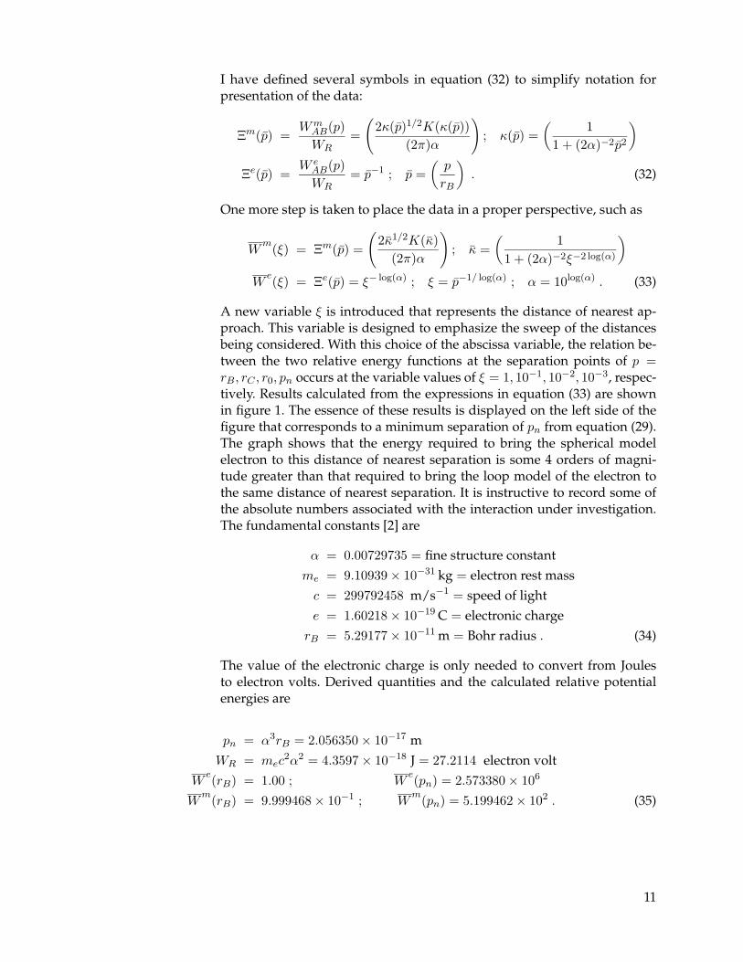
A new variable ξ is introduced that represents the distance of nearest ap-proach. This variable is designed to emphasize the sweep of the distancesbeing considered. With this choice of the abscissa variable, the relation be-tween the two relative energy functions at the separation points of p =rB, rC , r0, pn occurs at the variable values of ξ = 1, 10−1, 10−2, 10−3, respec-tively. Results calculated from the expressions in equation (33) are shownin figure 1. The essence of these results is displayed on the left side of thefigure that corresponds to a minimum separation of pn from equation (29).The graph shows that the energy required to bring the spherical modelelectron to this distance of nearest separation is some 4 orders of magni-tude greater than that required to bring the loop model of the electron tothe same distance of nearest separation. It is instructive to record some ofthe absolute numbers associated with the interaction under investigation.The fundamental constants [2] are
α = 0.00729735 = fine structure constant
me = 9.10939 × 10⁻³¹ kg = electron rest mass
c = 299792458 m/s−1 = speed of light
e = 1.60218 × 10⁻¹⁹ C = electronic charge
rB = 5.29177 × 10⁻¹¹ m = Bohr radius . (34)
The value of the electronic charge is only needed to convert from Joulesto electron volts. Derived quantities and the calculated relative potentialenergies are
pn = α3rB = 2.056350 × 10⁻¹⁷ m
WR = mec2α2 = 4.3597 × 10⁻¹⁸ J = 27.2114 electron volt
We(rB) = 1.00 ; W
e(pn) = 2.573380 × 10⁶
Wm(rB) = 9.999468 × 10⁻¹ ; W
m(pn) = 5.199462 × 10² . (35)
11

Figure 1. Relativeinteraction potentialenergy for two electronmodels.
10–3 10–2 10–1 10010–2
100
102
104
106
108
Position parameter (ξ)
Rel
ativ
e po
tent
ial e
nerg
y
Spherical modelLoop model
Absolute potential energies are
W eAB(rB) = 4.3597 × 10⁻¹⁸ J = 27.2114 electron volt
WmAB(rB) = 4.3594 × 10⁻¹⁸ J = 27.2100 electron volt
W eAB(pn) = 1.1219 × 10⁻¹¹ J = 70.0253 × 10⁶ electron volt
WmAB(pn) = 2.2668 × 10⁻¹⁵ J = 1.4148 × 10⁴ electron volt . (36)
Of particular interest in the results shown in equation (36) is the orderof magnitude of the energy that must be supplied to bring two electronsto within the separation distance of a fraction of the classical radius ofr0 = 2.8179 × 10⁻¹⁵ according to the two models. Whereas, the spheri-cal model indicates 70,000,000 electron volts, the loop model shows some14,000 electron volts.
12

7. Summary and Discussion of Results
The classical physics calculations of this report started with the sphericalshell model of the electron for which the classical radius is calculated byequating the electric-field energy to the measured electron rest mass en-ergy. Assuming this sphere was spinning fast enough to generate a mag-netic moment equal to its measured value, I showed that the peripheral ve-locity required would be many times the speed of light. Furthermore, I alsoshowed that the magnetic-field energy of such a magnetic moment wouldbe some 1000 times the rest mass energy. The quantity then sought was theradius of some object (probably a loop) whose peripheral velocity was nearthe speed of light (equal to it in the derivation) and, at the same time, giv-ing the correct magnetic moment and the correct magnetic-field energy. Theresulting object was a torus whose radius was proportional to the Comp-ton wavelength divided by 2π—the latter quantity is being referred to asthe magnetic radius rcl
m. The proportionality factor was the cube root of thenatural logarithm of the torus radius divided by the toroidal tube radiusrm. Selecting a value for this proportionality factor implied a rudimentarystructure. If the value selected is unity, then the tube radius is uncommonlysmall. If, on the other hand, a value is selected less than unity, while thetube radius is increased, the loop radius is decreased from the magnetic ra-dius, which in turn requires a peripheral velocity greater than the speed oflight. I calculated further results using the proportionality factor of unity.
At this point, I include modern experimental results in the calculations. Itis widely understood that high-energy electron-electron scattering experi-ments show that the scattering pattern is that of a point like entity downto several orders of magnitude less than the classical radius. Since the indi-cated tube radius rm is so small, the speculation arises as to the scatteringpattern of such a loop. The first step in such an investigation was performedin this report. The potential interaction energy was calculated under theassumption of only electric-field forces. The arrangement of the coaxial in-teracting loops was that their planes were parallel and that the directionof approach was perpendicular to these planes. Calculations showed thatthe potential energy of the spherical model was about 4 orders of magni-tude greater than that of the loop model at the nearest approach distancechosen. Thus, to the limited extent suggested by the primitive interactionscenario used in this report, the loop model results are in accordance withthe experimental results.
While no definitive theory has yet been applied to calculate interaction pa-rameters for alternate (and more realistic) scenarios, one can reach certainconclusions by starting from the nature of the force fields involved. Some ofthese conclusions concerning alternate scenarios pertinent to further workfollow:
13
• Scenario 1: Loops approach in planes perpendicular to approach line(electric and magnetic forces). Magnetic forces will have dramatic in-fluences, especially since the interaction force is attractive if the mag-netic moments are in the same direction. The relation between electricand magnetic forces as a function of separation is the priority calcula-tion needed because the results will show if magnetic forces must beused in the following scenarios. An aspect of this relation was indi-cated by an approximate calculation done some time ago. This calcu-lation was used to judge the radius of a charged torus tube necessaryfor the electric-field energy to be the rest mass energy. The rough re-sults showed this radius to be very small also. An improved calcula-tion of this effect has been included in appendix D, where it is indeedshown that the electric-field energy of a hollow torus is the electronrest mass energy. This information could not be used in this reportbecause an appropriate partition of the energy between the electricand magnetic fields has not been determined.
• Scenario 2: Loops approach “edge one” (electric field). The nearestapproach distance will be nearly twice the loop radius. Since the in-teraction force is higher for the nearest arc segments of the loops thanit is for the farther separated arc segments, the scenario is unstablebecause of the torque involved. Any alignment error will tend to in-crease the error until the loops are parallel. This unstable approachalignment will have a very low probability and therefore contributelittle to an averaged scattering cross section.
• Scenario 3: Loop centers on approach line—planes are not perpendu-lar to approach line (electric forces). Here also torque will be exertedon each loop by the field of the other because of the different distancesbetween loop segments. The torque will tend to rotate the loops intoparallel plane alignment at the point of nearest approach after whichthe torque will reverse the rotation. There is a dynamic effect here,since the torque depends upon the relative orientation angle, whichis the angle being changed by the integral of the torque times the mo-ment of inertia.
• Scenario 4: Loop center not on same approach line—planes have gen-eral orientation (electric field). This is the most general case for electric-field interactions. The dynamic effect here is enhanced because theloop offset greatly increases the torques. It is possible that in the lat-ter stages of the approach, each loop will be spinning. If this doesoccur, then the net force will be a function of time different from thatgiven by the static field variation as a function of separation only.
14

References
1. Goedecke, G. H., “Classically radiationless motions and possible impli-cations for quantum theory,” Phys. Rev. 135: (1B), 13 July 1964, pp B281–288.
2. Mohr, P. J., and B. N. Taylor, “CODATA recommended values of thefundamental physical constants: 1998,” Rev. Mod. Phys. 72 (2), April2000, pp 351–495.
3. Menzel, D. H., ed., Fundamental Formulas of Physics, Dover Publications,Inc., New York, 1960.
15


Appendix A. FY01 Director’s Research Initiative Proposal
File Number: FY01-CISD
Directorate: Computational and Information Sciences Directorate
Title: Radiationless Moving Charge and Current Distributions Using CluesFrom Semiclassical Static Electro-Magnitism
Principal Investigator: Dr. Harry J. Auvermann ([email protected]),U.S. Army Research Laboratory, Computational and Information SciencesDirectorate, Battlefield Environment Division, Atmospheric Acoustics andElectro-Optics Propagation Branch, AMSRL-CI-EP, Adelphi LaboratoryCenter, bldg 202, rm 4G102, ph 301-394-2088, fax 301-394-4797.
Objective: Determine if a magnetic model of the electron has scatteringproperties matching those measured in electron-electron colliding beamexperiments.
Technical Challenge/Background: When the Bohr atom is introduced in aphysics curriculum, derivation of the electron motion proceeds under theassumption that this moving charge does not radiate as it traverses the cir-cular or elliptical orbit, even though an accelerating charge is known toradiate energy according to Maxwell’s equations. I became aware of an ar-ticle published in 1964 [1] on radiationless charge-current distributions. Theauthor found that many such distributions exist. A necessary part of pro-ducing a radiationless model of the hydrogen atom is a radiationless modelof the electron.
I began a study of the properties of the electron starting with the deriva-tion of the classical radius. The semiclassical derivation for this quantityequates the static electric-field energy of a hollow sphere bearing the elec-tron charge to the rest mass energy. For my own benefit, I decided to inves-tigate the static magnetic-field energy of a spinning sphere whose radiusis the classical radius, thinking that the magnetic-field energy would bemuch less than the classical electric-field energy. Using my own approxi-mation for the magnetic-field energy, I was nevertheless very surprised tofind that the magnetic-field energy was some 900 times the electric-fieldenergy. Additionally, the peripheral velocity of the sphere had to be manytimes the speed of light to achieve the required magnetic moment.
Backing off from the classical radius requirement, I sought the radius ofa charged loop whose peripheral velocity was the speed of light but stillhad the correct magnetic moment and field energy. Using my calculation,although approximate, I determined the answer for the model loop ra-dius being what I call the Compton radius, or radius of a circle whose
17

circumference is the Compton wavelength. I determined also that the re-quired ”charged wire” radius (to give an electric-field energy for a Comp-ton radius-sized loop to be equal to the electron rest mass) was a numberso small that it defied imagination.
In the intervening years, an article appeared on a colliding-beam experi-ment (I believe at the European Organization for Nuclear Research) thatshowed the cross section for electron-electron scattering was at least a fac-tor of 100 less than the classical size. I have not verified or found the ref-erence to this article, but two colleagues have assured me that this resultis currently universally accepted in the particle physics community. Whenthe experiment report was published, in light of my ”charged wire” radiuscalculation, I theorized that I may be on the right track with my Comptonradius loop model.
Recently, I checked my past calculation. The effort proved surprisingly easywith the benefits of hindsight. The derivation used the commonly availableexpressions for the various physical constants [2–4]: the fine structure con-stant, the Bohr radius, the classical radius, the Bohr magneton, the Comp-ton wavelength, the rest mass energy, speed of light in terms of the per-meability and permittivity of free space, the magnetic moment of a currentloop, the free electron g-factor, the field energy of an inductor, and the in-ductance of a current loop. The radius was shown to be the Compton radiusmultiplied by the cube root of a factor consisting of the natural logarithmassociated with the inductance times the g-factor squared times the finestructure constant divided by 2π. Because this factor contained the loga-rithm of the ratio of the current loop radius to the ”wire radius” and wasto the one-third power, I set it equal to unity and solved for the ratio. Theapproximate value obtained was the natural base raised to the power 861.As I recall, the ratio I obtained previously for the charge loop was the natu-ral base raised to the power 234. These incredible exponent numbers comeabout through the reciprocal of the fine structure constant.
Relationship to ARL Mission: The relationship of this effort to the ARLmission is long-term but clearly established. When the U.S. Army firesnuclear weapons, radioactive cleanup is a vital activity on the battlefield.Therefore, the Army needs scientific backup in training and in equipmentprocurement to responsibly develop operational capability in this area. To aphysicist, development of this capability is a natural result of investigationssuch as is contained in this proposal. The three-element trail is a new un-derstanding of the (1) electron, (2) the atom, and (3) the nucleus. The newunderstanding arises from incorporating the idea of nonradiating chargeor current distributions into fundamental theory. Exploitation of the newidea of the magnetic energy of the electron begins a process whereby theArmy, besides attending to its own needs, gives back to the civilian andscientific community something potentially quite significant. To state thislong-term mission in a single paragraph is in no way intended to minimizethe difficulty expected when performing the work.
18

Approach: The first requirement is to study the appropriate literature rele-vant to the high-energy collider experiment result, which will provide theparameters for the theoretical analysis. The next step will be to establish thedifferences to be expected when a loop is substituted for one of the inter-acting spherical particles accounting only for electric-field effects. Step bystep, the theory will be expanded to the advanced relativistic scattering the-ory. Indications exist in the literature scanned so far that later experimentstook place with polarized particles [5].
It is almost certain that all the steps described here cannot be accomplishedin the one year allotted to projects funded under this program. These detailsare given to establish the overall progression of the intent and mind-set forthe work.
Tasks Milestones:
• Oct 00: Complete financial matters. Develop a detailed work plan.
• Jan 01: Complete scenario design. Complete electric-field study.
• Jun 01: Complete magnetic-field study. Begin high-energy study.
• Oct 01: Write final report with recommendations for follow-on work.
Benefits of Successful Completion: Successful completion implies that thetheoretical scattering studies are corroborated in some manner by the ex-perimental results. To the extent of this corroboration, a revised model ofan electron will be indicated. This revised model can then be used in amore elaborate theoretical scattering investigation than was possible dur-ing the limited time period originally allotted to a DRI project. Success inthis more elaborate venture will bring the postulation of a radiationlesselectron model nearer. Success can thus have a ripple effect on models foratoms, leptons other than the electron, baryons, and ultimately the nucleus.I would like to emphasize that these latter effects are complete specula-tion at present. Ultimate success would be knowledge of the nucleus elab-orate enough to suggest methods of radioactivity decay-rate modification[6], which would contribute to more efficient radioactive waste disposal.
Collaborations: Dr. George H. Goedecke, Department of Physics, New Mex-ico State University, Las Cruces, New Mexico, has agreed to collaborate onthis project. Dr. Goedecke is the author of the first article cited in the refer-ences to this proposal and has published later findings on the subject. Heis a recognized authority on scattering theory, both electromagnetic andquantum mechanical. He is also an author of many papers on other aspectsof modern physics. Dr. David A. Ligon of ARL, whose dissertation was inthe field of Quantum Electro Dynamics, has agreed to review progress ofthe work and provide insight within the limits of his other commitments.
19

Budget:
Salary: $60,000 Dr. H. J. Auvermann, six man months
Equipment: $0
Travel: $0
OGA: $0
Contract: $15,000 Dr. G. H. Goedecke, short-term analyticalservices
Other external: $0
Total cost: $75,000
Qualifications of Principal Investigator: Auvermann was awarded thePh.D. degree in Physics/Math in 1957 by the University of Texas at Austin.During most of his career, he has been working in the field of optics. Since1990, he has been Project Leader for the 6.1 Work Unit Battlefield AcousticPropagation Research. He initiated the creation of the Turbule EnsembleModel (TEM) of turbulence [7,8], supervised the insertion of TEM into theexisting two-dimensional Fast Field Program acoustic propagation model,and supervised the development of the Two-Way Wave Equation Model(TWWEM), a three-dimensional acoustic propagation model.
Literature Search: A search with the use of the elements electron-electronand scattering found some 1500 articles, 90 percent of which deal withsemiconductor physics. A search through Physical Review failed to locatethe article mentioned in the Technical Challenge/Background section. Areview article was found [9] as well as several articles on polarization ef-fects other than the one in the reference section [5].
20

References
1. Goedecke, G. H., “Classically radiationless motions and possible im-plications for quantum theory,” Phys. Rev. 135(1B) (1964), p B281.
2. Abramowitz, M., and I. A. Stegun, Handbook of Mathematical Functions,U.S. Government Printing Office, Washington, DC 20402 (1970).
3. Wolfe, William L., and George J. Zissis, The Infrared Handbook, U.S. Gov-ernment Printing Office, Washington, DC 20402 (1978).
4. Menzel, D. H., ed., Fundamental Formulas of Physics, Dover Publications,Inc., New York (1960).
5. Shieh, S. Y., “Electron-electron scattering cross section including polar-ization corrections,” Phys. Lett. B B26(4) (1968).
6. Anderson, J. L., J. Phy. Chem. 76 (1972), p 3603.
7. Goedecke, G. H., and H. J. Auvermann, “Acoustic scattering by atmo-spheric turbules,” J. Acoust. Soc. Am. 102(2), Pt. 1 (August 1997).
8. Goedecke, G. H., R. C. Wood, H. J. Auvermann, V. E. Ostashev, D. I.Havelock, and Chueh Ting, “Spectral broadening of sound scatteredby advecting atmospheric turbulence,” J. Acoust. Soc. Am. (May 2001).
9. Panofsky, W.K.H., “Some remarks on the early history of high-energyelectron-electron scattering,” Int. J. Mod. Phys. A 13(14) (1998), p 2429.
21


Appendix B. Magnetic Moment of a Spinning Charged Sphere
This appendix will be concerned with deriving an approximation to themagnetic moment of a spinning charged sphere. The method will be toconsider the sphere as being made up of a series of loops positioned onthe surface of the sphere and add up the contributions to the magnetizingforce-field contributions at the center of the sphere. The equivalent currentin a loop whose radius is the classical electron radius will be defined asthe current that gives the same magnetizing force at its center. The field HL
along the axis of a current loop is given by [1]
HL =ILr
2
2 [z2 + r2]3/2, (B-1)
where IL is the current in the loop and r is the radius of the loop.
The distance from the plane of the loop is the variable z. If the radius of thesphere is r0 and qa is the total charge, the surface charge density σ is
σ =qa
4πr20
. (B-2)
If the sphere center is at z = 0 and the angle φ is measured from the positivez-axis, quantities of interest are
r = r0 sin(φ); z = r0 cos(φ); I(φ)dφ =σ(2πr)(r0dφ)(Ωr)
(2πr)
HS =∫ π
0dφHL(φ) =
∫ π
0dφ
(I(φ)r2
2 [z2 + r2]3/2
). (B-3)
The variable HS is the field at the center of the sphere, and Ω is the angularvelocity. The constituents are brought together as
HS =∫ π
0dφHL(φ) =
(qaΩr0
4πr20
) ∫ π
0dφ
(r30 sin(φ)3
2r30 [cos(φ)2 + sin(φ)2]3/2
)
=(qaΩ6πr0
)(B-4)
and the integration performed. With equation (B-1) for z = 0 and the equiv-alent loop current Icl, the two are equated and solved for Icl as(
Iclr20
2r30
)=
(qaΩ6πr0
)
Icl =(qaΩ3π
). (B-5)
[1] Menzel, D. H., ed., Fundamental Formulas of Physics, Dover Publications, Inc., NewYork (1960), p 321.
23

Equation (B-5) gives the equivalent loop current for a sphere that carries acharge qa that rotates at an angular velocity of Ω. “Equivalent” means thatthe magnetic field at the center of the loop is the same as at the center of thesphere. The magnetic moment [2] is shown to be the current times the looparea. Thus the magnetic moment of a spinning charged sphere is
µs = 2πr20Icl =
(2r2
0qaΩ3
)=
(2r0qav
cl
3
), (B-6)
where vcl is the peripheral velocity of the equivalent current loop to thespherical shell.
[2] Menzel, D. H., ed., Fundamental Formulas of Physics, Dover Publications, Inc., NewYork (1960), p 323.
24
Appendix C. Potential Interaction Energy of Two Charged Loops
The interaction studied in this appendix is that of two charged coaxial cir-cular loops positioned with their planes parallel. The only force consideredis the static electric-field repulsion. The background suggesting the studyof the interaction of circular loops has been given in the main text. There thediscussion acknowledges the complicated nature of the total interaction ofcharged and current loops. The restricted interaction equations developedhere are intended as a precursor to an extended development to be accom-plished at a later date.
Consider the interaction diagram shown in figure C-1. In the figure, theA loop is in the x-y plane and the B loop is in a plane parallel to the x-yplane, with its center a distance zb = d above the origin O. The variousvectors marked by bold symbols are defined as
*ra = element position vector for A loop = xa cos(α) + ya sin(α)*rb = element position vector for B loop = xb cos(β) + yb sin(β) + zd (C-1)
*rab = *rb − *ra ,
where a is the radius of A loop and b is the radius of B loop. The differentialforce vector on the charge element at point *rb caused by the charge elementat point *ra is
d*Fab =
(1
4πε0r2ab
) (qaa dα
2πa
) (qbb dβ
2πb
)rab =
(qaqb dα dβ
(2π)24πε0r2ab
) (*rab
rab
)
rab = |*rb − *ra| =[a2 + b2 + d2 − 2ab cos(β − α)
]1/2. (C-2)
The total charges on the loops are qa and qb. After integration over the twoangles, the total force on B loop will be in the z direction. This is obtainedby forming the dot product of equation (C-2) and z with the result shownas
FAB =(
qaqbd
(2π)24πε0
) ∫ 2π
0dα
∫ 2π
0dβr−3
ab . (C-3)
After the α integration is done, the result will be the same for each β sothat the β integration will be trivial and β can be set to any value in the αintegration. The value is set to zero with the result shown as
25
Figure C-1. Interactiondiagram for twocharged loops (A andB). O = origin.
yx
ra
rab
α
B
A
z
βrb
O
→
→
→
FAB =(
qaqbd
(2π)4πε0
) ∫ 2π
0dα r−3
ab ; Let b =b
a; d =
d
a
=(
qaqbd
(2π)4πε0
) ∫ 2π
0dα
[a2 + b2 + d2 − 2ab cos(α)
]−3/2(C-4)
=
(2qaqbd
(2π)4πε0a2
) ∫ π
0dα
[1 + b2 + d2 − 2b cos(α)
]−3/2,
along with additional manipulation. The above integral is beginning tolook like a standard Elliptic Integral [1], so the variable of integration ischanged after use of a trigonometric identity with the result shown as
FAB =
(2qaqbd
(2π)4πε0a2
) ∫ π/2
0dθ
[(1 − b)2 + d2 + 4b sin2(θ)
]−3/2. (C-5)
At this point, the identity of the two loops is recognized with the resultingform
FAB =
(4q2
a
(2π)4πε0d2
) ∫ π/2
0dθ
[1 + D2 sin2(θ)
]−3/2; D = 2d−1 . (C-6)
If this force is integrated from infinity to a particular distance p, then theresult will be minus the potential energy Wm
AB(p) of B loop in the field ofA loop and is shown as
WmAB(p) =
∫ p
∞dd′FAB = −
(4q2
a
(2π)4πε0
) ∫ p
∞
(dd′
d′2
) ∫ π/2
0dθ
[1 + D2 sin2(θ)
]−3/2. (C-7)
It appears that the distance 2a has a special role to play, so the variable ofthe integration will be changed to a unitless quantity with the use of 2a asa parameter as
26

WmAB(p) =
(−4q2
a
(2π)4πε0
) ∫ p
∞
(dd′
d′2
) ∫ π/2
0dθ
[1 + D2 sin2(θ)
]−3/2; η =
d′
2a
WmAB(q) =
(−2q2
a
(2π)4πε0a
) ∫ q
∞
(dη
η2
) ∫ π/2
0dθ
[1 + η−2 sin2(θ)
]−3/2; q =
p
2a(C-8)
= −CAB
∫ q
∞
(dη
η2
) ∫ π/2
0dθ
[1 + η−2 sin2(θ)
]−3/2; CAB =
(2q2
a
(2π)4πε0a
).
With the anticipation of later investigations, the above integral deservesspecial attention because the value of the parameter q is to be chosen sothat the point of closest approach is to be in the range to match the experi-mental results. With α now representing the fine-structure constant and therecognition of the loop radius to be the magnetic radius rcl
m or the Comptonradius, the classical radius is α rcl
m. The closest approach should be some100 times smaller than the classical radius. Therefore, for theoretical pur-poses, q will be thought of as equal to α2. It is necessary to break up theintegration into two intervals as
WmAB(q) =
WmAB(q)CAB
= −(L1 + L2)
L1 =∫ 1
∞
(dη
η2
) ∫ π/2
0dθ
[1 + η−2 sin2(θ)
]−3/2(C-9)
L2 =∫ q
∞
(dη
η2
) ∫ π/2
0dθ
[1 + η−2 sin2(θ)
]−3/2,
where the relative potential energy WmAB(q) has been defined also. Solution
of the integral L1 proceeds by an inversion of the order of integration as
L1 =∫ 1
∞
(dη
η2
) ∫ π/2
0dθ
[1 + η−2 sin2(θ)
]−3/2=
∫ π/2
0dθ
∫ 1
∞
dηη[
η2 + sin2(θ)]3/2
= −∫ π/2
0dθ
[1 + sin2(θ)
]−1/2= −K(−1) = −2−1/2K
(12
), (C-10)
where K(m) is the Complete Elliptic Integral of the First Kind [1]. Solutionof integral L2 proceeds as
L2 =∫ q
1
(dη
η2
) ∫ π/2
0dθ
[1 + η−2 sin2(θ)
]−3/2=
∫ π/2
0dθ
∫ q
1
dηη[
η2 + sin2(θ)]3/2
= −∫ π/2
0dθ
[q2 + sin2(θ)
]−1/2−
[1 + sin2(θ)
]−1/2
(C-11)
= −(
1(1 + q2)1/2
) ∫ π/2
0dθ
[(q2
(1 + q2)
)+
(sin2(θ)(1 + q2)
)]−1/2
− L1 ,
[1] Wolfram Research, Mathematica 3.0 Standard Add-On Packages, Wolfram Media,Champaign, IL 61820 (1996).
27
with additional manipulations such as
L2 = −(
1(1 + q2)1/2
) ∫ π/2
0dθ
[1 −
(1
(1 + q2)
)cos2(θ)
]−1/2
− L1
= −(
1(1 + q2)1/2
) ∫ π/2
0dθ
[1 −
(1
(1 + q2)
)sin2(θ)
]−1/2
− L1 (C-12)
= −(
1(1 + q2)1/2
)K(k) − L1 ; k = (1 + q2)−1 .
Equation (C-13) presents the major result of this derivation
WmAB(p) =
(2k1/2q2
aK(k)(2π)4πε0a
); k = (1 + q2)−1 ; q =
p
2a, (C-13)
which is the expression for the potential energy of two loop model electronspositioned as in figure C-1.
28
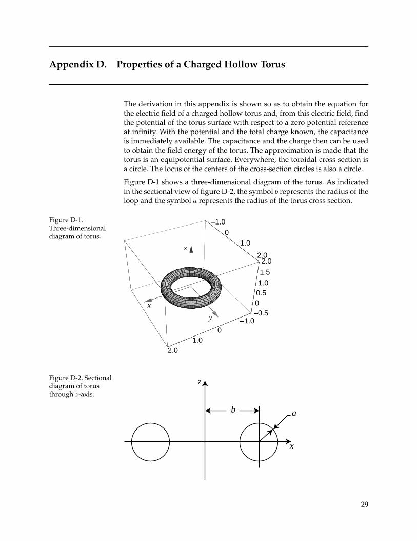
Appendix D. Properties of a Charged Hollow Torus
The derivation in this appendix is shown so as to obtain the equation forthe electric field of a charged hollow torus and, from this electric field, findthe potential of the torus surface with respect to a zero potential referenceat infinity. With the potential and the total charge known, the capacitanceis immediately available. The capacitance and the charge then can be usedto obtain the field energy of the torus. The approximation is made that thetorus is an equipotential surface. Everywhere, the toroidal cross section isa circle. The locus of the centers of the cross-section circles is also a circle.
Figure D-1 shows a three-dimensional diagram of the torus. As indicatedin the sectional view of figure D-2, the symbol b represents the radius of theloop and the symbol a represents the radius of the torus cross section.
Figure D-1.Three-dimensionaldiagram of torus.
–1.00
1.0
2.02.0
1.51.0
0.50–0.5
–1.00
1.02.0
x
z
y
Figure D-2. Sectionaldiagram of torusthrough z-axis.
b a
x
z
29

The formula for the surface area of a torus is given in equation (D-1) [1]. Inthe formula
At = π2(b′2 − a′2
)(D-1)
from the reference, the symbol a′ is the inner radius of the torus and thesymbol b′ is the outer radius of the torus. With the translation of the equa-tion (D-1) formula to the parameters of figure D-2, the equation (D-2) for-mula is obtained:
At = (2π)2ab . (D-2)
Letting the symbol qt represent the total charge on the torus, the surfacecharge density σt is
σt =(qt
At
)=
(qt
(2π)2ab
). (D-3)
For the electric field to be found, the electric-flux density D is related to thesurface charge density and the direction is assumed normal to the surface.Since the surface is assumed equipotential and since the field is a conserva-tive one, the potential can be obtained by integration of the field along anypath from infinity to the surface. The path along the positive x-axis is cho-sen for its comparative simplicity. By symmetry, this path represents anystraight line path in the x-y plane. If the symbol r represents the positionalong the x-axis, then the integration is from r = ∞ to r = a + b.
To find the flux density at a point r on the x-axis, assume that a rectangulardetector D centered on the x-axis (and perpendicular to it) has a dimensionw in the y direction and a dimension h in the z direction. The object is tofind the dimensions of the patch on the near surface from which issues theflux intercepted by D. This flux will be augmented by the flux that issuesfrom the patch on the far surface. The far surface is the inner part of thetorus, which is on the other side of the z-axis from the near surface. Sym-bols with the subscript n will apply to the near patch, and symbols withthe subscript f will apply to the far patch. Only these two patches needbe considered. Justification for this conclusion is discussed later in this ap-pendix. Determination of patch dimensions is facilitated by two diagrams.The first is shown in figure D-3, which depicts the situation in the x-z plane.The rays from the near patch appear to come from the center, marked Cn,of the right-hand trace of the surface in this plane. The detector subtendsan angle αn from this point. The rays from the far patch appear to comefrom the center, marked Cf , of the left-hand trace of the toroidal surface.The detector subtends an angle αf from this point.
Equation (D-4) shows the calculation of these two-patch dimensions:
αn =(
h
r − b
); hn =
(ha
r − b
)
αf =(
h
r + b
); hf =
(ha
r + b
). (D-4)
[1] Spiegel, M. R., Mathematical Handbook of Formulas and Tables, Schaum’s Outline Series,McGraw-Hill, Inc., New York (1968), 34th Printing (1995), p 10.
30

Figure D-3. Patchdimensions in x-z plane.
Cf
hf
αf
z
hn
αn
D
h x
x = rCn
The second patch dimension diagram is shown in figure D-4, which depictsthe situation in the x-y plane. The rays from both patches appear to comefrom the loop center, which is the coordinate system origin. This is seeneasily for the near patch. It is also true for the far patch, because the normalrays tend to focus the flux at the origin in this plane. The detector subtendsan angle βn from this point for the near patch. The detector subtends anangle βf for the far patch. Although for βn = βf , the patch dimensions aredifferent.
The calculation of these two-patch dimensions is
βn =(w
r
); wn =
(w(b + a)
r
); wf =
(w(b− a)
r
). (D-5)
The flux from the entire charge in a patch proceeds outward, as justifiedat the end of this appendix. The partial flux at the detector from the twopatches designated by ∆FD is
∆FD = σt(hnwn + hfwf ) =
=(
qt
(2π)2ab
) ((hb
r − a
) (w(a + b)
r
)+
(hb
r + a
) (w(a− b)
r
)). (D-6)
The electric-flux density is then obtained by dividing the flux by the detec-tor area as
D(r) =(
qt
(2π)2ar
) ((a + b
r − a
)+
(a− b
r + a
)). (D-7)
Dividing by the electric constant ε0 gives the electric field as
E(r) =(
2qt
(2π)2ε0r
) (r + b
r2 − a2
)=
(2[1 + (b/r)]
π
) (qt
4πε0(r2 − a2)
). (D-8)
At great distances where r is much greater than a or b, the electric field isseen to be the same as that from a point charge except for the 2/π factor inthe first bracket. To obtain the potential φt, assume that the charge is pos-itive and accumulate the energy necessary to move a unit positive chargefrom infinity to r = a + b through the field of equation (D-8) as
φt =(
2π
) (qt
4πε0
) ∫ a+b
∞dr
(r + b
r(r2 − a2)
). (D-9)
31

Figure D-4. Patchdimensions in x-yplane.
Cf
Wf
y
CnWn
βn
D
xw
x = r
To solve the integral, substitute for the variable of integration a tan(θ) as
φt = Qt
∫ θt
π/2dθ
(sec(θ)2[tan(θ) + b/a]tan(θ)[tan(θ)2 − 1]
); θt = arctan(1 + b/a)
=(Qt
a
) ∫ θt
π/2dθ
([a sin(θ) + b cos(θ)]
sin(θ) cos(2θ)
); Qt =
(2π
) (qt
4πε0a
). (D-10)
Further manipulations are carried out by
φt =
(Qt
(a2 + b2
)1/2
a
) ∫ π4+δ
π/2dθ
(sin(θ + γ)
sin(θ) cos(2θ)
); θt =
π
4+ δ
tan(γ) =b
a; tan
(π
4+ δ
)= 1 + b/a ; tan(δ) =
(b/a
2 + b/a
). (D-11)
The integration result is shown as [2]
I =∫ π
4+δ
π/2dθ
(sin(θ + γ)
sin(θ) cos(2θ)
)
=(
12
) cos(γ) ln
[cos(δ)sin(δ)
]+ sin(γ) ln
[(cos(δ) + sin(δ))2
4 cos(δ) sin(δ)
] (D-12)
=(
12(a2 + b2)1/2
) a ln
[a
b
]+ b ln
[(2a + b)(a + b)
2ab
] .
Substituting in equation (D-11), the final expression for the potential is
φt =(
1π
) (qt
4πε0a
) ln
[a
b
]+
(b
a
)ln
[(2a + b)(a + b)
2ab
]
=(
1π
) (qt
4πε0a
) (1 +
b
a
)ln
[a
b
]+
(b
a
)ln
[(1 +
b
2a
) (1 +
b
a
)] . (D-13)
For large a/b (and small b/a), the ln(a/b) term is dominent so that an ap-proximate potential is given by
φt =(
1π
) (qt
4πε0a
)ln
[a
b
]. (D-14)
[2] Wolfram, S., MATHEMATICA, 2nd ed., Addison-Wesley, New York (1991).
32

The equation for the capacitance C is [3]
C =q
∆φ; Ct =
qt
φt(D-15)
in terms of the charge q and the potential difference ∆φ. The capacitanceCt of the torus is also shown in equation (D-15). The energy W stored in acapacitance [3] is given in two forms as
W =C(∆φ)2
2=
q2
2C. (D-16)
With the use of the second form and substituting quantities defined inequation (D-13), the formula for the electric-field energy of the torus Wt
is shown as
Wt =q2t
2Ct
=(
12π
) (q2t
4πε0a
) (1 +
b
a
)ln
[a
b
]+
(b
a
)ln
[(1 +
b
2a
) (1 +
b
a
)] . (D-17)
It is instructive to use the approximate formula for the torus potential,equation (D-14), to obtain an idea of the magnitude of this electric-fieldenergy for the torus configuration calculated in the main text of this report.The approximate value for the electric-field energy of the torus Wt is
Wt =(
12π
) (q2t
4πε0a
)ln
[a
b
]. (D-18)
From equation (23) in the main text, the loop radius is given as the Comptonradius, and from equation (26), the approximate value of the loop parame-ter ρm is given. These values are shown as
rC
rt= ρm = exp
(2πα
). (D-19)
The variable rC is identified with the variable b in equation (D-18), andthe variable rt is identified with the variable a in equation (D-18). With theappropriate substitutions made in equation (D-18), the result is shown as
Wt =(
12π
) (q2t
4πε0rC
)ln
[rC
rt
]=
(12π
) (q2t
4πε0rC
) (2πα
). (D-20)
Consolidating equation (D-20) and noting the relation between the Comp-ton radius and the classical radius r0 from equation (7) in the main text, onecan show the result as
Wt =
(q2t
4πε0r0
)= we . (D-21)
[3] Menzel, D. H., ed., Fundamental Formulas of Physics, Dover Publications, Inc., NewYork (1960), p 318.
33

The final identification is made with we of equation (8) in the main text,which is the rest mass energy of the electron. Thus we find that the approx-imate electric-field energy of the present configuration of the hollow torusis the same as that of the classical electron model. This information has onlybeen mentioned in the main text of this report because an appropriate allo-cation of the rest mass energy between the electric and magnetic fields hasnot been determined.
That only two patches are needed for finding the electric field of a torusmay be concluded by considering the situation wherein charge radiateselectric flux both outward (as with the derivation just shown) and inward.The reduction in flux by a factor of two is made up by the inclusion offour patches instead of two. In reference to figure D-3, the focusing effectin the z-direction causes the flux from the left-hand patches of the tubes tobe redistributed onto the right-hand patches, thus effectively augmentingthe outward-moving flux. In figure D-4, this same effect occurs in the y-direction. The inward-moving flux from the left-hand portion of the torusmoves through the focus point (the coordinate origin) and redistributes it-self on the right-hand portion of the torus. A further point can be madeconcerning the net flux within the torus: With flux being focused in bothdirections inside the torus, the net flux at each point balances to zero infigure D-3, indicating zero field, considering only one circle. The effect ofthe flux from one circle on the other circle has not been included. Thus, theassumption that the surface is equipotential only becomes true as the ratioa/b approaches zero. In figure D-4, in the x-y plane, the focused flux fromboth sides balances to zero everywhere inside the loop, again indicatingzero field in this plane.
34

35
Distribution
AdmnstrDefns Techl Info CtrATTN DTIC-OCP8725 John J Kingman Rd Ste 0944FT Belvoir VA 22060-6218
DARPAATTN S Welby3701 N Fairfax DrArlington VA 22203-1714
Mil Asst for Env Sci Ofc of the Undersec ofDefns for Rsrch & Engrg R&AT E LS
Pentagon Rm 3D129Washington DC 20301-3080
Ofc of the Secy of DefnsATTN ODDRE (R&AT)The PentagonWashington DC 20301-3080
Ofc of the Secy of DefnsATTN OUSD(A&T)/ODDR&E(R) R J Trew3080 Defense PentagonWashington DC 20301-7100
AMCOM MRDECATTN AMSMI-RD W C McCorkleRedstone Arsenal AL 35898-5240
US Army TRADOCBattle Lab Integration & Techl DirctrtATTN ATCD-BFT Monroe VA 23651-5850
US Military AcdmyDept of Mathematical SciATTN MAJ L G EggenWest Point NY 10996-1786
US Military AcdmyMathematical Sci Ctr of ExcellenceATTN MADN-MATH MAJ M HuberThayer HallWest Point NY 10996-1786
Natl Ground Intllgnc CtrArmy Foreign Sci Tech CtrATTN CM220 7th Stret NECharlottesville VA 22901-5396
Natl Security AgcyATTN W21 Longbothum9800 Savage RdFT George G Meade MD 20755-6000
Dir for MANPRINTOfc of the Deputy Chief of Staff for PrsnnlATTN J HillerThe Pentagon Rm 2C733Washington DC 20301-0300
Sci & Technlgy101 Research DrHampton VA 23666-1340
SMC/CZA2435 Vela Way Ste 1613El Segundo CA 90245-5500
TECOMATTN AMSTE-CLAberdeen Proving Ground MD 21005-5057
US Army ARDECATTN AMSTA-AR-TDBldg 1Picatinny Arsenal NJ 07806-5000
US Army Corps of EngrsEngr Topographics LabATTN CETEC-TR-G P F Krause7701 Telegraph RdAlexandria VA 22315-3864
US Army CRRELATTN CRREL-GP R Detsch72 Lyme RdHanover NH 03755-1290

Distribution (cont’d)
36
US Army Dugway Proving GroundATTN STEDP 3Dugway UT 84022-5000
US Army Field Artillery SchlATTN ATSF-TSM-TAFT Sill OK 73503-5000
US Army InfantryATTN ATSH-CD-CS-OR E DutoitFT Benning GA 30905-5090
US Army Info Sys Engrg CmndATTN AMSEL-IE-TD F JeniaFT Huachuca AZ 85613-5300
US Army Natick RDECActing Techl DirATTN SBCN-T P BrandlerNatick MA 01760-5002
US Army OECATTN CSTE-AEC-FSE4501 Ford Ave Park Center IVAlexandria VA 22302-1458
US Army Simulation Train & InstrmntnCmnd
ATTN AMSTI-CG M MacedoniaATTN J Stahl12350 Research ParkwayOrlando FL 32826-3726
US Army Soldier & Biol Chem CmndDir of Rsrch & Techlgy DirctrtATTN SMCCR-RS I G ResnickAberdeen Proving Ground MD 21010-5423
US Army Tank-Automtv Cmnd RDECATTN AMSTA-TR J ChapinWarren MI 48397-5000
US Army TRADOCAnal Cmnd—WSMRATTN ATRC-WSS-RWhite Sands Missile Range NM 88002
US Army TRADOCATTN ATCD-FAFT Monroe VA 23651-5170
Nav Air War Cen Wpn DivATTN CMD 420000D C0245 A Shlanta1 Admin CirChina Lake CA 93555-6001
Nav Surfc Warfare CtrATTN Code B07 J Pennella17320 Dahlgren Rd Bldg 1470 Rm 1101Dahlgren VA 22448-5100
Nav Surfc Weapons CtrATTN Code G63Dahlgren VA 22448-5000
USAF Rsrch Lab Phillips LabAtmos Sci Div Geophysics DirctrtHanscom AFB MA 01731-5000
US Air ForceATTN Weather Techl Lib151 Patton Ave Rm 120Asheville NC 28801-5002
USAF Rome Lab TechATTN Corridor W Ste 262 RL SUL26 Electr Pkwy Bldg 106Griffiss AFB NY 13441-4514
NASA Marshal Spc Flt CtrAtmos Sci DivATTN Code ED 41 1Huntsville AL 35812
Hicks & Assoc IncATTN G Singley III1710 Goodrich Dr Ste 1300McLean VA 22102
Natl Ctr for Atmos RsrchATTN NCAR Library SerialsPO Box 3000Boulder CO 80307-3000

37
Distribution (cont’d)
NCSUATTN J DavisPO Box 8208Raleigh NC 27650-8208
Pacific Mis Test Ctr Geophysics DivATTN Code 3250Point Mugu CA 93042-5000
US Army Rsrch LabATTN AMSRL-IS-EWWhite Sands Missile Range NM 88002-5501
DirectorUS Army Rsrch LabATTN AMSRL-RO-D JCI ChangATTN AMSRL-RO-EN W D BachPO Box 12211Research Triangle Park NC 27709
US Army Rsrch LabATTN AMSRL-D D R SmithATTN AMSRL-DD J M MillerATTN AMSRL-CI-AI-R Mail & Records
MgmtATTN AMSRL-CI-AP Techl Pub (2 copies)ATTN AMSRL-CI-LL Techl Lib (2 copies)ATTN AMSRL-CI-EP H J Auvermann
(15 copies)Adelphi MD 20783-1197


1. AGENCY USE ONLY
8. PERFORMING ORGANIZATION REPORT NUMBER
7. PERFORMING ORGANIZATION NAME(S) AND ADDRESS(ES)
12a. DISTRIBUTION/AVAILABILITY STATEMENT
10. SPONSORING/MONITORING AGENCY REPORT NUMBER
5. FUNDING NUMBERS4. TITLE AND SUBTITLE
6. AUTHOR(S)
REPORT DOCUMENTATION PAGE
3. REPORT TYPE AND DATES COVERED2. REPORT DATE
11. SUPPLEMENTARY NOTES
14. SUBJECT TERMS
13. ABSTRACT (Maximum 200 words)
Form ApprovedOMB No. 0704-0188
(Leave blank)
9. SPONSORING/MONITORING AGENCY NAME(S) AND ADDRESS(ES)
Public reporting burden for this collection of information is estimated to average 1 hour per response, including the time for reviewing instructions, searching existing data sources,gathering and maintaining the data needed, and completing and reviewing the collection of information. Send comments regarding this burden estimate or any other aspect of thiscollection of information, including suggestions for reducing this burden, to Washington Headquarters Services, Directorate for Information Operations and Reports, 1215 JeffersonDavis Highway, Suite 1204, Arlington, VA 22202-4302, and to the Office of Management and Budget, Paperwork Reduction Project (0704-0188), Washington, DC 20503.
12b. DISTRIBUTION CODE
15. NUMBER OF PAGES
16. PRICE CODE
17. SECURITY CLASSIFICATION OF REPORT
18. SECURITY CLASSIFICATION OF THIS PAGE
19. SECURITY CLASSIFICATION OF ABSTRACT
20. LIMITATION OF ABSTRACT
NSN 7540-01-280-5500 Standard Form 298 (Rev. 2-89)Prescribed by ANSI Std. Z39-18298-102
An Elementary Electron Model for Electron-ElectronScattering Based On Static Magnetic Field Energy
February 2001 Final, June to August 2000
Electron motion paths that exhibit zero radiation in a Maxwell’s equation solution have beenreported. Such paths, require a radiationless model of the electron itself, such as the chargedhollow sphere. When the electric-field energy of this model is set equal to the rest mass energy ofthe electron, the radius of the resulting sphere is called the “classical electron radius.” Analysisreveals that the static magnetic-field energy of the classical model is many times the electron restmass energy when the sphere is given an angular velocity large enough to exhibit the electronmagnetic moment. The necessary angular velocity produces a peripheral velocity many times thespeed of light. A classical model with a peripheral velocity near the speed of light is a loopwhose radius is the Compton wavelength divided by 2π; such a loop has a very small dimensionperpendicular to the loop plane. Experiments reveal point-like electron scattering properties downto at least 1/100 of the classical radius. The small transverse dimensions of the loop model indicatesimilar scattering results. Recently, a proposal was submitted to investigate the scatteringproperties of interacting loops. Because of limited proposal length, derivation of loop modelequations could not be included. This report contains the details of the analysis.
Current loop, classical scattering, rest mass energy
Unclassified
ARL-TR-2332
OFEJ6061110253A11
B53A61102A
ARL PR:AMS code:
DA PR:PE:
Approved for public release; distributionunlimited.
42
Unclassified Unclassified UL
2800 Powder Mill RoadAdelphi, MD 20783-1197
U.S. Army Research LaboratoryAttn: AMSRL-CI-EP [email protected]
U.S. Army Research Laboratory
39
Harry J. Auvermann
email:2800 Powder Mill RoadAdelphi, MD 20783-1197