an ellipsoidal calculus based on propagation and fusion ... · an ellipsoidal calculus based on...
TRANSCRIPT

430 IEEE TRANSACTIONS ON SYSTEMS, MAN, AND CYBERNETICS—PART B: CYBERNETICS, VOL. 32, NO. 4, AUGUST 2002
An Ellipsoidal Calculus Based on Propagationand Fusion
Lluís Ros, Assumpta Sabater, and Federico Thomas
Abstract—This paper presents an Ellipsoidal Calculus basedsolely on two basic operations: propagation and fusion. Propaga-tion refers to the problem of obtaining an ellipsoid that must satisfyan affine relation with another ellipsoid, and fusion to that of com-puting the ellipsoid that tightly bounds the intersection of two givenellipsoids. These two operations supersede the Minkowski sum anddifference, affine transformation and intersection tight boundingof ellipsoids on which other ellipsoidal calculi are based. Actually,a Minkowski operation can be seen as a fusion followed by a prop-agation and an affine transformation as a particular case of propa-gation. Moreover, the presented formulation is numerically stablein the sense that it is immune to degeneracies of the involved ellip-soids and/or affine relations.
Examples arising when manipulating uncertain geometric infor-mation in the context of the spatial interpretation of line drawingsare extensively used as a testbed for the presented calculus.
Index Terms—Ellipsoidal bounds, ellipsoidal calculus, set-mem-bership uncertainty description.
I. INTRODUCTION
M OST techniques for parameter estimation assume that thedata are corrupted by random noise whose probability
density function is usually assumed to be gaussian. Real-worlduncertainties, however, also include nongaussian, nonwhitenoise and systematic errors. These uncertainties can easily beconsidered in a set theoretic setting which consists in definingbounds for the uncertain variables [23]. Fortunately, both set the-oreticandprobabilistic techniquescanbecombined,asdescribedin [7], to cope with situations where the uncertainty is describedpartly by bounds and partly by probability density functions.
The main problem with the set theoretic description of un-certainty is that, although the initial uncertainty sets have simpleshapes, the results of principal operations with them have a com-plicated shape. This is why some canonical sets, that depend ona fixed number of parameters, are introduced for the approxi-mation of uncertainty sets. The problem that arises here is toapproximate the results of the operations by means of canonicalsets with maximal accuracy. Among many possibilities, ellip-soids are usually taken as these canonical sets because they
a) can be concisely described;b) provide a satisfactory approximation of convex sets in
most applications;
Manuscript received April 6, 2001; revised January 26, 2002. This work wassupported in part by the Spanish CICYT under Contract TIC2000-0696. Thispaper was recommended by Associate Editor R. Santos.
L. Ros and F. Thomas are with the Industrial Robotics Institute (CSIC-UPC),Barcelona 08028, Spain (e-mail: [email protected]; [email protected]).
A. Sabater is with the Applied Mathematics Department, Polytechnical Uni-versity of Catalonia, Terrassa 08222, Spain (e-mail: [email protected]).
Publisher Item Identifier S 1083-4419(02)03115-1.
c) can be represented using matrices interpretable asweighted covariance matrices;
d) are invariant, as a class, under affine transformations.The basic operations traditionally needed to deal with ellip-
soidal uncertainty sets have been
a) Minkowski sum of ellipsoids;b) Minkowski difference of ellipsoids;c) affine transformations of ellipsoids;d) intersection of ellipsoids.
These four operations are required in many contexts otherthan set theoretic uncertainty manipulation, such as optimiza-tion and approximation, identification and experiment plan-ning, probability and statistics, adaptive control, mathematicalmorphology, etc. Then, because of their relevance, the term El-lipsoidal Calculus has been coined to refer to these operationsas a set [9].
This paper first deals with the problem of obtaining an ellip-soid which satisfies a given affine relation with another ellip-soid, by means of an operation calledpropagationwhich can beseen as a generalization of the elementary affine transformationof ellipsoids. Then, it tackles the problem of obtaining the ellip-soid with minimum volume among those resulting from a linearconvex combination of two possibly degenerate ellipsoids, anoperation calledfusion which provides a suboptimal solutionto the problem of finding the ellipsoid with minimum volumecontaining the intersection of the two ellipsoids defining theconvex combination. Finally, it shows how the computation ofMinkowski sums and differences of ellipsoids can be performedby fusions followed by propagations. Altogether, this leads to analternative Ellipsoidal Calculus, with a reduced number of op-erations, that can supersede previous ones.
The presented formulation was motivated by the followingproblem arising when manipulating uncertain geometric fea-tures [18], [16]. Suppose that the ellipsoidal uncertainty regionsassociated with the parameter vectorsand are known,and that we also know that both vectors are related throughthe vector equation . Then, any information onprovides information on , at least in part, and vice versa. Theproblem is to combine both uncertainty sets to obtain a new set,either for or , that takes into account that they are mutuallyconstrained. This problem cannot be solved using ordinaryellipsoidal calculi based on the four aforementioned operations.This can be easily shown by noting that, even in the case thatone of the parameter vectors has a bounded uncertainty region,the induced uncertainty set for the other may be unboundedin some directions, and that the result of the four operationsis always bounded for bounded inputs. This problem can beeffectively solved using propagations and fusions [6].
1083-4419/02$17.00 © 2002 IEEE

ROSet al.: ELLIPSOIDAL CALCULUS BASED ON PROPAGATION AND FUSION 431
Although the affine transformation of ellipsoids is a trivialproblem, the more general one of obtaining an ellipsoid thatsatisfies an affine relation with another ellipsoid, in the pres-ence of possible degeneracies, is by no means trivial. Whilstthis problem has received little attention in the literature, the oneof computing an ellipsoid containing the intersection of two el-lipsoids has been investigated at least since the sixties [8]. Inthe early eighties, the exact solution to this problem was onlyknown in the particular case in which one of the ellipsoids de-generates into a half-space. The technique proposed in [4] forcomputing an ellipsoid containing the intersection of two ellip-soids consists in computing the tangent plane at a point on oneof the two ellipsoids. This plane defines a halfspace that canbe used to approximate the ellipsoid itself. Then, an ellipsoidbounding the intersection between this halfspace and the otherellipsoid roughly approximates the intersection of both ellip-soids. A refinement on this consists in taking an initial ellipsoidlarge enough to contain the intersection and computing tangentplanes on both ellipsoid boundaries to obtain halfspaces that areiteratively intersected with the result [12]. The process is re-peated, possibly with the same set of halfspaces, until no signifi-cant reduction in the volume is observed. This way of improvingthe result by recirculating the data of half-space batches, as longas it reduces the volume of the result, has been broadly appliedin the context of set description of uncertainty, but it will not ingeneral produce a globally optimal ellipsoid. This motivated thedevelopment of the globally optimal minimal-volume algorithmdescribed in [14]. Another alternative consists in distributing aset of points on both ellipsoid boundaries, and removing thosefrom one ellipsoid that are not contained in the other. Then, theproblem consists in obtaining the smallest ellipsoid containingall surviving points, using for example the algorithms describedin [25] or [21]. This is one of the techniques used in the commer-cially available software described in [22]. All these approaches,that can be said to be based on discretizations, obviously fail towork properly when at least one of the ellipsoids is degenerate.
The problem of bounding the intersection of two concentricellipsoids is much simpler because the optimum is necessarilyin the family of linear convex combinations of both ellipsoids[8]. This reduces the problem to the minimization of a functionin a single variable. Even if both ellipsoids are not concentric,we can still look for the optimum in this family but then theresult is just a suboptimum that curiously satisfies most of thedesirable properties for the optimum. Although Schweppe [20]already mentioned the interest of finding the best ellipsoid inthis family in the sense of various criteria including its volume,he provided no way of computing the optimum. This was doneabout ten years later by Fogel and Huang for the volume andtrace criteria, in the case of an ellipsoid an the region defined bytwo parallel hyperplanes—which can be seen as a degenerateellipsoid. Belforte and Bona [2] showed that when one of thehyperplanes does not cut the original ellipsoid, the volume ofthe resulting ellipsoid using the Fogel-Huang algorithm can bereduced by substituting a parallel hyperplane tangent to the orig-inal ellipsoid for the nonintersecting hyperplane. This provedthat the Fogel–Huang algorithm was not optimal. In the con-text of linear programming, an algorithm was developed to ob-tain a minimum-volume ellipsoid containing the intersection of
an ellipsoid with a half-space or a region limited by two par-allel hyperplanes [3]. It has been shown that the Fogel-Huangalgorithm, as modified by Belforte and Bona is mathematicallyequivalent to the minimal-volume ellipsoid using this linear pro-gramming technique and therefore optimal [14]. Maksarov andNorton explored further this approach in [11], where they finallygive a function whose single root in the range of interest givethe minimum volume ellipsoid within the linear convex combi-nation of two ellipsoids. This technique is used in [22], whereit is shown to provide tighter results than using discretizations,as expected. Nevertheless, the obtained function is not definedif both ellipsoids are degenerate, even in the case their inter-section is bounded, and in its expression appears inverses ofmatrices that depend on the function variable. We here give analternative derivation that concludes with a polynomial whosecomputation avoids matrix inversions that can lead to numer-ical ill-conditionings. Moreover, the degeneracy of both ellip-soids is not an impediment to its direct application, provided thattheir intersection is bounded, a circumstance that can be easilychecked beforehand. Nevertheless, both formulations must pro-vide the same result, at least when both ellipsoids are not de-generate. In particular, if one of the ellipsoids degenerates intoa region defined by two parallel hyperplanes, both methods mustbe equivalent to the Fogel–Huang algorithm. We have providedthis equivalence by algebraic manipulations of our polynomial.We also prove that our expression has a single root in the rangeof interest by the more straightforward technique of proving theconvexity of the volume function.
The first attempt to find the minimal-volume ellipsoid con-taining the Minkowski sum of two ellipsoids was done in [4],but the used derivation was quite complicated. A neater one wasgiven in [11]. We here show how a Minkowski set operation canalways be expressed in terms of a fusion followed by a propa-gation.
This paper is structured as follows. The next section includesthe notations, definitions and all the mathematical backgroundneeded throughout this paper. Sections III and IV are devote thepropagation and fusion operation, respectively. Section V con-tains the examples, including Minkowski set operations carriedout by degenerate fusions followed by propagations. Finally,Section VI concludes with points that deserve further research.
II. BACKGROUND
A. Notation
Matrices.-th entry of matrix .
Identity matrix.Vectors.Transpose of .Matrix of cofactors of .Inverse of .Right inverse of .Left inverse of .Pseudoinverse of .Orthogonal complement of .Rank of .Trace of .

432 IEEE TRANSACTIONS ON SYSTEMS, MAN, AND CYBERNETICS—PART B: CYBERNETICS, VOL. 32, NO. 4, AUGUST 2002
Determinant of .Subspace spanned by the rows of.Orthogonal subspace to that of .Positive square root of.
B. Ellipsoids
A real -dimensional ellipsoid, centered on, can be con-cisely described as
(1)
where is a positive-semidefinite symmetric matrix.Imaginary ellipsoids, which may appear when manipulating realellipsoids, can analogously be described as
can be diagonalized into the form, where are the eigen-
values of and the columns of , are thecorresponding orthonormal eigenvectors. The principal axes ofthe ellipsoid are the directions given by and its semiaxeslengths are given by .
The volume of is given by
(2)
where is the volume of the unit ball in .By definition we will assign a negative volume to imaginary
ellipsoids such that
(3)
When is singular, i.e., its rank is lower thaneigenvalues are zero, the corresponding semiaxes lengths tendto infinity and so does the volume defined by (2) and (3). In thiscase, (1) is better said to correspond to anelliptical cylinder inwhich the affine variety is defined as itsvarietyof centersbecause remains invariant if is substi-tuted by any point of this variety. In the particular case in which
, (1) represents a region bounded by two parallelhyperplanes, orstrip, whose variety of centers is a hyperplanelocated just in the middle of the bounding hyperplanes.
From the diagonalized form of, it can be shown that canalways be expressed as , where the columns ofare being the eigenvectors corresponding to nonnulleigenvalues. Then, if is an full columnrank matrix. For example, for a strip of width .
C. Definitions and Properties
Definition 1 (Right and Left Inverse): is a right inversematrix of if, and only if, . Likewise, is a leftinverse matrix of if, and only if, .
Right and left inverses have the following properties.
1) Given and do not always exist and, if they exist,in general they are not unique.
2) If is not singular, then .3) has right inverse if and only if it has full row rank. Then
its right inverse matrix has full column rank. Likewise,
has left inverse if and only if it has full column rank andthen its left inverse matrix has full row rank.
4) If has full row rank, is a rightinverse matrix of . And, if has full column rank,
is a left inverse matrix of .
Definition 2 (Orthogonal Complement):Let be anfull row rank matrix, then any full column
rank matrix satisfying is called an orthogonalcomplement of .
is called the orthogonal complement of because. Since the columns of form a basis of the
nullspace of , it can be readily obtained from the singularvalue decomposition of .
Lemmma 1:Let be a full row rank matrix, then
there exists such that .
Proof: Sinceis a nonsingular matrix and
exists. Let us see that . Since
is an orthogonal complement of . .Therefore, there exists a matrix satisfying . Inaddition, . Hence, .
Definition 3 (Pseudoinverse): is called the pseudoinverseof if, and only if, , and both,
and , are symmetric.Pseudoinverse matrices have the following properties.
1) If is square and nonsingular, then . Other-wise, there will be infinitely many .
2) If has a right inverse, then is a right inverse. Like-wise, if has a left inverse, then is a right inverse.
3) If the system has solution, then is asolution.
Pseudoinverses of ellipsoid matrices can be easily computedfrom their eigenvectors since .
III. PROPAGATION
This section considers the problem of obtaining the set thatmust satisfy an affine relation with a given possibly degenerateellipsoid. We constructively show that this set is also an ellip-soid thus generalizing, using pseudoinverses, the straightfor-ward affine transformation of ellipsoids. This problem ariseswhenever two parameter vectorsand are known to be re-lated through a vector equation . Then, their cor-responding uncertainty regions are obviously related. By lin-earizing this equation at , we obtain
which is an affine equation of the type . It ispossible to introduce an uncertainty region associated withtoaccount for the residuals of the linearization. Nevertheless, forthe sake of simplicity, is assumed to be constant in this section.The general case involves the computation of Minkowski sumand thus a fusion of ellipsoids which is explained in the nextsection.

ROSet al.: ELLIPSOIDAL CALCULUS BASED ON PROPAGATION AND FUSION 433
Fig. 1. Geometric interpretation of ellipsoid propagation.
Definition 4 (Ellipsoid Propagation):The propagation ofthrough the mapping
(4)
is defined as the set
where are and matrices, respectively, of rank.For mapping (4) to define a relation betweenand andmust have the same rank. On the contrary, ifhad rank
smaller, or larger, than , it would constrain the coordinates of, or , respectively. The assumption thatand are full row
rank matrices is not restrictive as (4) can always be simplifiedby row operations such that the involved matrices have full rowrank.
Let be a point satisfying . Then, theequation defining the mapping (4) is equivalent to
Hence, the mapping (4) can be expressed as the following com-position of mappings:
This composition can be seen as a projection followed by anextension by simply identifying with the linear subspace of
defined by the rows of , and the linear subspace ofdefined by the rows of , respectively (Fig. 1).
Theorem 1 (Propagation):The propagation of ellipsoidthrough the mapping
defined by the equation , where, is the ellipsoid ,
where is a point satisfying and.
Proof: First, we propagate through, or equivalently through ,
to obtain .Since has full row rank, according to Lemma 1, there exists
such that , where .
Then, can be expressed as
Changing variables , we get
that is
(5)
This inequality defines an ellipsoid in the space for con-stant values of whose center, , satisfies
. Using pseudoinverses, one solution to thisequation is . Then, the ellipsoidgiven by (5) can be rewritten as
Since it should correspond to a real ellipsoid, its independentterm has to be positive, i.e.
Substituting and rearranging terms, we get
Then, the propagated ellipsoid matrix is
Finally, we have to propagate throughto obtain . Since if, and only if,
we conclude that .
IV. FUSION
The ellipsoidal approximation of the exact intersections oftwo ellipsoids should be obtained from the minimization of ameasure that reflects its geometrical size. The measures usuallyconsidered for this minimization are: the volume (which corre-sponds to the maximization of the ellipsoid matrix determinant),the sum of squares of the semiaxes (which corresponds to theminimization of the trace of the ellipsoid matrix inverse), andthe length of the largest semiaxis (which corresponds to maxi-mization of the smallest eigenvalue of the ellipsoid matrix). Fora comparison of the results obtained when bounding the inter-section of an ellipsoid and a strip using the trace versus the de-terminant criterion the reader is addressed to [5]. We will usethe volume criterion because it is the one that better reflects theintuitive idea of tight bounding.
Theorem 2: Given two possibly degenerate ellipsoids,and , whose intersection is a nonempty
bounded region, the region defined by
(6)
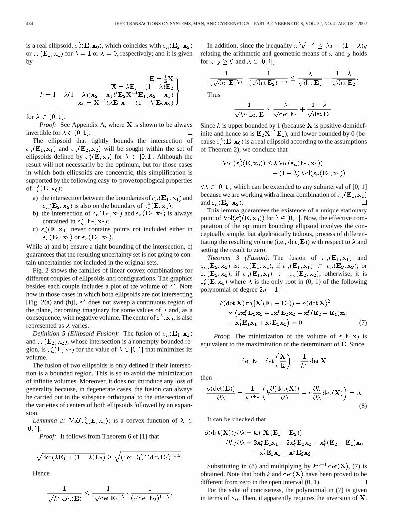
434 IEEE TRANSACTIONS ON SYSTEMS, MAN, AND CYBERNETICS—PART B: CYBERNETICS, VOL. 32, NO. 4, AUGUST 2002
is a real ellipsoid, , which coincides withor for or , respectively; and it is givenby
for .Proof: See Appendix A, where is shown to be always
invertible for .The ellipsoid that tightly bounds the intersection of
and will be sought within the set ofellipsoids defined by for . Although theresult will not necessarily be the optimum, but for those casesin which both ellipsoids are concentric, this simplification issupported by the following easy-to-prove topological propertiesof :
a) the intersection between the boundaries of andis also on the boundary of ;
b) the intersection of and is alwayscontained in ;
c) never contains points not included either inor .
While a) and b) ensure a tight bounding of the intersection, c)guarantees that the resulting uncertainty set is not going to con-tain uncertainties not included in the original sets.
Fig. 2 shows the families of linear convex combinations fordifferent couples of ellipsoids and configurations. The graphicsbesides each couple includes a plot of the volume of. Notehow in those cases in which both ellipsoids are not intersecting[Fig. 2(a) and (h)], does not sweep a continuous region ofthe plane, becoming imaginary for some values ofand, as aconsequence, with negative volume. The center of , is alsorepresented as varies.
Definition 5 (Ellipsoid Fusion): The fusion ofand , whose intersection is a nonempty bounded re-gion, is for the value of that minimizes itsvolume.
The fusion of two ellipsoids is only defined if their intersec-tion is a bounded region. This is so to avoid the minimizationof infinite volumes. Moreover, it does not introduce any loss ofgenerality because, in degenerate cases, the fusion can alwaysbe carried out in the subspace orthogonal to the intersection ofthe varieties of centers of both ellipsoids followed by an expan-sion.
Lemmma 2: is a convex function of.Proof: It follows from Theorem 6 of [1] that
Hence
In addition, since the inequalityrelating the arithmetic and geometric means ofand holdsfor and
Thus
Since is upper bounded by 1 (becauseis positive-demidef-inite and hence so is ), and lower bounded by 0 (be-cause is a real ellipsoid according to the assumptionsof Theorem 2), we conclude that
, which can be extended to any subinterval of [0, 1]because we are working with a linear combination ofand .
This lemma guarantees the existence of a unique stationarypoint of for . Now, the effective com-putation of the optimum bounding ellipsoid involves the con-ceptually simple, but algebraically tedious, process of differen-tiating the resulting volume (i.e., ) with respect to andsetting the result to zero.
Theorem 3 (Fusion):The fusion of andis: , if ; or
, if ; otherwise, it iswhere is the only root in (0, 1) of the following
polynomial of degree
(7)
Proof: The minimization of the volume of isequivalent to the maximization of the determinant of. Since
then
(8)
It can be checked that
Substituting in (8) and multiplying by , (7) isobtained. Note that both and have been proved to bedifferent from zero in the open interval (0, 1).
For the sake of conciseness, the polynomial in (7) is givenin terms of . Then, it apparently requires the inversion of.

ROSet al.: ELLIPSOIDAL CALCULUS BASED ON PROPAGATION AND FUSION 435
Fig. 2. Fusion examples.
Nevertheless, since and the second termof (7) is multiplied by the dividing terms cancel andno numerical ill-conditionings are possible.
In Fig. 2, the graphs of and of (7) are plottedin function of , for several ellipse families. Clearly, the rootof (7) in the interval (0, 1) coincides with the value ofthatminimizes the volume of . The ellipse corresponding to this
root is highlighted in thick line in every family. The trajectoryof the center as varies is also indicated.
Corollary 1: When the centers of both ellipsoids coincide,, and the problem can be reduced to obtain the
roots of the following polynomial of degree

436 IEEE TRANSACTIONS ON SYSTEMS, MAN, AND CYBERNETICS—PART B: CYBERNETICS, VOL. 32, NO. 4, AUGUST 2002
Fig. 3. (a) An incorrect truncated tetrahedron. To be correct,x ; x andxshould coincide, as illustrated in (b).
Proof: If and . Substitutingin (18), (22) is obtained.
Note that the fusion of two degenerate ellipsoids whose vari-eties of centers intersect in a single point can be reduced to thiscase because this point is necessarily the center of the fused el-lipsoid.
Corollary 2: Ifis given by
where .Proof: See [19].
This corollary is useful to obtain the uncertainty region asso-ciated with the cartesian product of and ,i.e., a tight bounding of .It will be used in the examples below.
Corollary 3: When one of the ellipsoids is a strip, (7) reducesto a second order polynomial for which the sought root can beexplicitly computed.
Proof: See Appendix B for a proof of this corollary, wherethe result is also shown to be equivalent to the formula used bythe ellipsoid algorithm.
V. EXAMPLES
A. A Truncated Tetrahedron
Consider the line drawing in thick lines of Fig. 3(a). Supposeit has been obtained from a picture of a plane-faced object withan image processing system that, using a vertex extraction algo-rithm, has located within a disk of radius three pixelsaround each of the following positions:
Note that for this drawing to be a correct projection of a trun-cated tetrahedron, the three edge-lines , and
must all be concurrent to the same point, the apex of the (imag-inary) original tetrahedron [Fig. 3(b)]. In fact, for an arbitrarypolyhedron, one has a collection of suchconcurrence condi-tions, which, if satisfied on the projection, guarantee its correct-ness [15], [24].
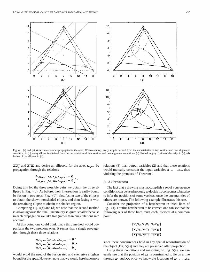
Fig. 4(a) and (c) show one possible way to verify the correct-ness of this drawing, based on computing an uncertainty regionfor the imaginary apex. This is done by first using the propa-gation operation repeatedly [Fig. 4(a)] to separately derive theuncertainty regions of
1) a point aligned with and ;2) a point aligned with and ;3) a point aligned with and ;
and then, using the fusion operation [Fig. 4(c)] to intersect thethree uncertainties together. If this intersection is nonempty, theline drawing can be judged as practically correct and we can starta 3-D reconstruction from it [17]. Otherwise, the six vertices aretoo badly placed and we can consider the use of some correctionalgorithm to take them over correct locations [16].
Since three points are aligned if and only if the determinantof their homogeneous coordinates is zero, the uncertainty of apoint aligned with two other points and can be easilycomputed by propagation through the relation
a relation which we will refer to as .Here, the input and output variables areand , respectively. The linearization of this rela-tion at a point is , with
The input ellipsoid for is easily derived by computing an ellip-soidal bound for the cartesian product of the uncertainty disksfor and , via the fusion operation (see Corollary 2 above).As expected, in each of the three propagations the output el-lipsoid for is a strip, as shown in Fig. 4(a). Finally, thesethree strips can be fused together to obtain the apex uncertainty[Fig. 4(c)]. This fusion is performed in two steps.
1) A first fusion involving the vertical and one of the obliquestrips in Fig. 4(a), to derive the nonshaded ellipse inFig. 4(c).
2) A second fusion of this ellipse with the other oblique stripin Fig. 4(a), to obtain the shaded ellipse in Fig. 4(c).
A second way of computing the apex uncertainty is shown inFig. 4(b) and (d). Here, we use the fact that the apex point mustlie on the intersection of any pair of the three edge-lines
, and . Thus, we can select any two of these lines, say
ROSet al.: ELLIPSOIDAL CALCULUS BASED ON PROPAGATION AND FUSION 437
Fig. 4. (a) and (b) Vertex uncertainties propagated to the apex. Whereas in (a), every strip is derived from the uncertainties of two vertices and one alignmentcondition; in (b), every ellipse is obtained from the uncertainties of four vertices and two alignment conditions. (c) Shaded in grey: fusion of the strips in (a); (d)fusion of the ellipses in (b).
and and derive an ellipsoid for the apex bypropagation through the relations
Doing this for the three possible pairs we obtain the three el-lipses in Fig. 4(b). As before, their intersection is easily boundby fusion in two steps [Fig. 4(d)]: first fusing two of the ellipsesto obtain the shown nonshaded ellipse, and then fusing it withthe remaining ellipse to obtain the shaded region.
Comparing Fig. 4(c) and (d) we note that the second methodis advantageous: the final uncertainty is quite smaller becausein each propagation we take two (rather than one) relations intoaccount.
At this point, one could think that a third method would out-perform the two previous ones: it seems that a single propaga-tion through these three relations
would avoid the need of the fusion step and even give a tighterbound for the apex. However, note that we would here have more
relations (3) than output variables (2) and that these relationswould mutually constrain the input variables , thusviolating the premises of Theorem 1.
B. A Hexahedron
The fact that a drawing must accomplish a set of concurrenceconditions can be used not only to decide its correctness, but alsoto infer the positions of some vertices, once the uncertainties ofothers are known. The following example illustrates this use.
Consider the projection of a hexahedron in thick lines ofFig. 5(a). For this hexahedron to be correct, one can see that thefollowing sets of three lines must each intersect at a commonpoint
since these concurrences hold in any spatial reconstruction ofthe object [Fig. 5(a)] and they are preserved after projection.
Using these conditions and reasoning on Fig. 5(a), we caneasily see that the position of is constrained to lie on a linethrough and , once we know the locations of .

438 IEEE TRANSACTIONS ON SYSTEMS, MAN, AND CYBERNETICS—PART B: CYBERNETICS, VOL. 32, NO. 4, AUGUST 2002
Fig. 5. Uncertainty regions forx ;x ; andx , given the input uncertainties ofx ; . . . ;x (depicted as small shaded disks around these vertices). Taking intoaccount the concurrence conditions in (b), we get the strips and ellipses in (e) and (g), depending on how these concurrences are specified (see the text). Using theconditions in (d), we get the strips and ellipses in (f) and (h).

ROSet al.: ELLIPSOIDAL CALCULUS BASED ON PROPAGATION AND FUSION 439
Thus, using propagation, we can deduce an ellipsoidal uncer-tainty for assuming that are known to lie withina disk of radius eight pixels around each of these locations
For this, we need a relation stating the concurrence of threelines, which we next derive. A line through two points,and
, can be characterized by itsPlücker coordinates, i.e., thethree 2 2 minors of the 2 3 matrix
Moreover, one can see that three lines are concurrent if, and onlyif, their Plücker coordinate vectors are linearly dependent. Thus,the three lines and are concurrent whenever
a condition which we will compactly refer to as
The linearization of this relation is , with
The partial derivatives of have simple expres-sions. For example, is equal to
Then, the uncertainty of can be derived by computing thecartesian product of the uncertainties of and prop-agating the resulting ellipsoid through the linearization of therelations
(9)
taking
as input and output variables, respectively. Note that, since theoutput is six-dimensional, we get the uncertainties ofand combined together. Thus we need to project this higherdimensional ellipsoid onto the planes , and
, to obtain two-dimensional uncertainty regions foreach point. Fortunately, such a projection can be seen as aspecial case of propagation: note that the projection of a point
onto coordinates, say , is the point
, where is an matrix all of whose entries arezero, except for , that are set to one.Hence the projection of an ellipsoid onto these coordinates, isachieved by applying Theorem 1 with and
.The results of such projections are shown in Fig. 5(e). As ex-
pected, we obtain a strip for the uncertainty of, and two par-allel strips, one for and the other for . We obtain stripsrather than ellipsoids for and because the chosen set ofrelations only constrains these points to lie on a line through theintersection points of lines and , on the one hand, and
and , on the other. However, the formulation is richenough to derive fully bounded ellipses forand . Namely,we need only express the same concurrences differently, propa-gating the same input ellipsoid through the relations
(10)
using the same vectorsand of input and output variables.The resulting uncertainties are depicted in Fig. 5(g).
Furthermore, if instead of a strip we need a fully boundedellipse for , we can always use the fact that the hexahedronmust accomplish the additional concurrence condition shown inFig. 5(c) and (d), so that we can add the relation
to the above relations (9) and (10) and perform the corre-sponding propagations again. The results are shown in Fig. 5(f)and (h), respectively, where the ellipse for is nondegenerateanymore.
C. Minkowski Set Operations
Let us suppose that we want to compute the uncertainty regionassociated with , where and
. can be expressed as
(11)
where . Then, the first step is to compute the uncer-
tainty region associated with. This can actually be seen as thefusion of two elliptical cylinders in . Then, using Corollary2, it is straightforward to prove that
where and .
It simply remains to propagate through (11),to obtain the Minkowski sum of and .Also, note that the Minkowski difference betweenand is just the Minkowski sum of and
.This has been implemented and several examples are shown
in Fig. 6. Every example displays two ellipsoids and comparestheir exact Minkowski sum with the ellipsoid bound obtained

440 IEEE TRANSACTIONS ON SYSTEMS, MAN, AND CYBERNETICS—PART B: CYBERNETICS, VOL. 32, NO. 4, AUGUST 2002
Fig. 6. (a)–(c) Minkowski sums of nondegenerate ellipsoids. (d)–(f) Minkowski sums of degenerate ellipsoids.
by the process above. The exact Minkowski sum of two ellipsesand can be obtained by first translatingto the origin, then overlaying copies of
around its contour, with fixed orientation, and finally translatingthe whole figure an amount . The envelope of the re-sulting family of ellipses is the desired Minkowski sum. Usingthis geometric construction we see in Fig. 6 that the Minkowskiset operation of our calculus obtains quite good approximations(in shaded grey) as compared to the exact sum (the envelope ofthe shown ellipse families). In the sequence of the first row wesee how the ellipsoidal and exact sums evolve, as the two el-lipses flatten to approximate a segment. In the second row weshow Minkowski sums of degenerate ellipsoids. Fig. 6(d) showsthe sum of an ellipse with a vertical strip of semiaxis length0.5, which results in a wider vertical strip of semiaxis length1.59. Fig. 6(e) depicts the sum of two strips of semiaxis length0.2, symmetrically placed about the-axis. The result is a stripof semiaxis length 0.4 that coincides with the exact Minkowskisum of the original sets. Finally, Fig. 6(f) shows the Minkowskisum of two oblique strips which returns the whole plane as ex-pected.
VI. CONCLUSION
The class of nondegenerate ellipsoids is closed under the al-lowed operations by ordinary ellipsoidal calculi. We have shownin this paper that the inclusion of degeneracies enlarge the class
and new operations—such as propagation—are now possible.Propagation has been defined as the operation of computing anellipsoid that satisfies an affine relation of the form
with another ellipsoid. We have limited our formulationto those cases in which and have the same rank, otherwiseconstraints on the coordinates ofor are introduced. This iswhy a fusion could be seen as a propagation where these ranksare different. This observation would allow us to introduce anEllipsoidal Calculus solely based on a single operation: a propa-gation without limitations on the ranks of the involved matrices.This point deserves further attention. Secondly, although it isconsidered a solved problem [9], [10], [13], further investiga-tion could also be carried out on the issue of inner approxima-tions, i.e., lower ellipsoidal bounds on the data. Since we knowthe exact result of a propagation, we only need to concentrateourselves on getting such bounds for the fusion operation, as aMinkowski sum or difference is just a combination of these twooperations.
Bounded-error data naturally lead to set estimates whichare an attractive alternative to point estimates, as derivedwhen using stochastic characterizations. The size of these setestimates will obviously depend on the quality of the datacollected. Among all feasible experiments, one may thereforebe interested in selecting the one which can be expected tominimize this size in some sense. This problem of experimentdesign has received a considerable amount of attention ina statistical context and it has also been considered in the

ROSet al.: ELLIPSOIDAL CALCULUS BASED ON PROPAGATION AND FUSION 441
bounded-error context. Nevertheless, up to our knowledge,its application to active sensing in Robotics, while certainlydeserving some attention, remains unexplored.
Finally, it is also worth to mention that an implementationin Maple of the presented Ellipsoidal Calculus as well as ex-amples, including those in this paper, can be downloaded fromhttp://www.iri.upc.es/people/ros/ellipsoids.html.
APPENDIX A
The set in (6) can be rewritten as
(12)
Then, its center, , is a solution of
where ,We now prove that can be inverted because
never vanish in the open interval (0, 1). Since bothellipsoids intersect in a bounded region, .Now, let us assume that but
. Then, there exists such that
Multiplying it by , we get
(13)
Since, for values of in the open interval (0, 1), the lhs of (13)is greater or equal to zero and its rhs lower or equal to zero, itis only satisfied if, and only if, simultaneously and
. That is, . Hence, since and are
symmetric matrices, , contrary
our assumption.Now, (12) can be rewritten as where
and
or, equivalently, after further algebraic tedium
We know that this corresponds to a real ellipsoid because italways contains the intersection. Then, sincecan be easilyproved to be positive-semidefinite,is always positive.
APPENDIX B
When using the ellipsoid method, a strip is usually describedas . If it is seen as a degenerate ellipsoid, it canbe expressed as , where
, and is any point satisfying .Then, from Theorem 3, the linear convex combination of this
strip and an arbitrary nondegenerate ellipsoid, say ,is , where
(14)
for . Note that we here use a different parameteriza-tion but, by setting and , the one inTheorem 3 is recovered.
Moreover, according to Theorem 4, the optimum boundingellipsoid within this family is obtained for a value ofsatisfying
(15)
where . A quite involved and tedious algebraicmanipulation allows us to express (15) as
(16)
where
and can be interpreted as the Mahalanobis distances in-duced by from to the hyperplanes and
, respectively.Since (16) is a second order polynomial in, its solutions are
where
Only the negative value for corresponds to a positive valuefor . Thus, the obtained solution for, once substituted in (14),leads to the equations used by the ellipsoid method for boundingthe intersection of an ellipsoid and a strip, as summarized in [3].
REFERENCES
[1] E. F. Beckenback and R. Bellman,Inequalities. Berlin, Germany:Springer-Verlag, 1961.
[2] G. Belforte and B. Bona, “An improved parameter identification al-gorithm for signals with unknown-but-bounded errors,” inProc. 7thIFAC/IFORS Symp. Identification Syst. Parameter Estimation, 1985, pp.1507–1512.
[3] R. G. Bland, D. Goldfard, and M. J. Todd, “The ellipsoid method: Asurvey,”Oper. Res., vol. 29, pp. 1039–1091, 1981.
[4] F. L. Chernousko, “Ellipsoidal bounds for sets of attainability and un-certainty in control problems,”Optim. Control Applicat. Meth., vol. 3,pp. 187–202, 1982.
[5] C. Durieu, B. T. Polyak, and E. Walter, “Trace versus determinant in el-lipsoidal outer-bounding, with application to state estimation,” inProc.IFAC World Congr., San Francisco, CA, 1996, pp. 43–48.

442 IEEE TRANSACTIONS ON SYSTEMS, MAN, AND CYBERNETICS—PART B: CYBERNETICS, VOL. 32, NO. 4, AUGUST 2002
[6] E. Fogel and Y. F. Huang, “On the value of information in system identi-fication—bounded noise case,”Automatica, vol. 18, no. 2, pp. 229–238,1982.
[7] U. D. Hanebeck and J. Horn, “Fusing information simultaneouslycorrupted by uncertainties with known bounds and random noise withknown distribution,”Inform. Fusion, no. 1, pp. 55–63, 2000.
[8] W. Kahan, “Circumscribing an ellipsoid about the intersection of twoellipsoids,”Can. Math. Bull., vol. 11, no. 3, pp. 437–441, 1968.
[9] A. Kurzhanski and I. Vályi,Ellipsoidal Calculus for Estimation andControl. Boston, MA: Birkhäuser, 1997.
[10] A. Kurzhanski and I. Varaiya, “Ellipsoidal techniques for reachabilityanalysis: The internal approximations,”Syst. Contr. Lett., vol. 41, pp.201–211, 2000.
[11] D. G. Maksarov and J. P. Norton, “State bounding with ellipsoidal setdescription of the uncertainty,”Int. J. Contr., vol. 65, no. 5, pp. 847–866,1996.
[12] M. Milanese and G. Belaforte, “Estimation theory and uncertainty inter-vals evaluation in the presence of unknown but bounded errors: Linearfamilies of models and estimates,”IEEE Trans. Automat. Contr., vol.AC-27, pp. 408–414, Feb. 1982.
[13] J. P. Norton, “Recursive computation of inner bounds for the parametersof linear models,”Int. J. Contr., vol. 50, no. 6, pp. 2423–2430, 1989.
[14] L. Pronzato and E. Walter, “Minimal volume ellipsoids,”Int. J. Adapt.Contr. Signal Process., vol. 8, pp. 15–30, 1994.
[15] L. Ros, “A kinematic-geometric approach to spatial interpretation ofline drawings,” Ph.D. dissertation, Polytech. Univ. Catalonia, Catalonia,Spain, 2000. [Online] Available: http://www-iri.upc.es/people/ros.
[16] L. Ros and F. Thomas, “Overcoming superstrictness in line drawing in-terpretation,”IEEE Trans. Pattern Anal. Machine Intell., vol. 24, Apr.2002.
[17] , “Numerical analysis of the instantaneous motions of panel-and-hinge frameworks and its application to computer vision,” inProc. 2ndWorshop Computat. Kinematics, 2001, pp. 199–210.
[18] A. Sabater and F. Thomas, “Set membership approach to the propaga-tion of uncertain geometric information,”Proc. IEEE Int. Conf. Robot.Automat., pp. 2718–2723, 1991.
[19] A. Sabater, “Propagation and fusion of uncertain geometry with boundederrors,” Ph.D. Dissertation, Polytechnical Univ. Catalonia, Spain, 1996.(in Catalan).
[20] F. C. Schweppe,Uncertain Dynamic Systems. Englewood Cliffs, NJ:Prentice-Hall, 1973.
[21] N. Z. Shor and O. A. Berezovski, “New algorithms for constructing op-timal circumscribed and inscribed ellipsoids,”Opt. Meth. Softw., vol. 1,pp. 283–299, 1992.
[22] S. M. Veres, A. V. Kuntsevich, I. Vályi, S. Hermsmeyer, D. S. Wall,and S. Sheng, “Geometric bounding toolbox for MATLAB,” inMATLAB/Simulink Connections Catalogue. Natick, MA: MathWorksInc., 2001.
[23] E. Walter and H. Piet-Lahanier, “Estimation of parameter bounds frombounded-error data: A survey,”Math. Comput. Simul., no. 32, pp.449–468, 1990.
[24] W. Whiteley, “Weavings, sections and projections of spherical poly-hedra,”Discr. Appl. Math., no. 32, pp. 275–294, 1991.
[25] E. Welzl, “Smallest enclosing disks (balls and ellipsoids),” inNew Re-sults and New Trends in Computer Science, H. Maurer, Ed. New York:Springer-Verlag, 1991, pp. 359–370.
Lluís Ros received the M.S. degree in mechanical engineering and the Ph.D.degree (with honors) in industrial engineering, both from the Polytechnic Uni-versity of Catalonia, Barcelona, Spain, in 1992 and 2000, respectively.
From 1993 to 1996, he was with the Control of Resources Group, CyberneticsInstitute, Barcelona, Spain, involved in the application of constraint logic pro-gramming to the control of electric and water networks. Since August 2000, hehas been a Research Scientist in the Industrial Robotics Institute, Spanish HighCouncil for Scientific Research. His current research interests are in geometryand kinematics, with applications to robotics, computer graphics and machinevision.
Assumpta Sabaterreceived the B.Sc. degree in mathematics from the Univer-sity of Barcelona, Spain, in 1984 and the Ph.D. degree in mathematics from thePolytechnical University of Catalonia, Terrassa, Spain, in 1996.
Since 1984, she has been a Staff Member at the Applied Mathematics III De-partment, Polytechnical University of Catalonia. Her research interests are inmathematics applied to robotics, with special emphasis on sensor integrationand uncertainty manipulation. She also works on mathematics applied to sus-tainable development.
Federico Thomasreceived the B.Sc. degree in telecommunications engineeringand the Ph.D. degree (with honors) in computer science, both from the Poly-technic University of Catalonia, Barcelona, Spain, in 1984 and 1988, respec-tively.
Since March 1990, he has been a Research Scientist in the Industrial RoboticsInstitute, Spanish High Council for Scientific Research. His research interestsare in geometry and kinematics, with applications to robotics, computergraphics, and machine vision. He has published more than 40 research papersin international journals and conferences.