an empirical study on weak-form of market efficiency of ... 2_2_5.pdf · an empirical study on...

Journal of Applied Finance & Banking, vol.2, no.2, 2012, 99-148 ISSN: 1792-6580 (print version), 1792-6599 (online) International Scientific Press, 2012

An Empirical Study on Weak-Form of Market

Efficiency of Selected Asian Stock Markets

Nikunj R. Patel1, Nitesh Radadia2 and Juhi Dhawan3

Abstract

The purpose of this research is to investigate the weak form of market efficiency

of Asian four selected stock markets. We have taken a daily closing price of stock

markets under the study from the 1st January 2000 to 31st March 2011 and also

divided full sample in three interval periods, and have applied various test like

Runs Test, Unit Root Test, Variance Ratio, Auto Correlation and other test. BSE

Sensex has given the highest mean returns to the investor followed by SSE

Composite and HANGSENG. BSE Sensex could be considered as high risk

markets as it has reported the highest Standard Deviation. During the period BSE

Sensex, HANGSENG and SSE Composite markets showed positive average daily

returns except NIKKEI. The Runs Test indicated BSE Sensex and NIKKEI

markets are weak form inefficient whereas HANSENG and SSE Composite hold

weak form of efficiency. The time series for the full as well as sample period did

1 S.V. Institute of Management, Kadi, e-mail:[email protected] 2 S.V. Institute of Management, Kadi, e-mail: [email protected] 3 S.V. Institute of Management, Kadi, e-mail: [email protected] Article Info: Received : January 21, 2012. Revised : February 16, 2012 Published online : April 15, 2012

100 A Study on Weak-Form of Market Efficiency of Asian Stock Markets

not have a presence of unit root in the markets understudy. According to Auto

correlation test it is inferred that the equity markets of the Asian region under the

study remained inefficient for some lag whereas they were efficient for the other

lag.

JEL classification numbers: C12, C14, D53, G14, G15

Keywords: Weak form Market Efficiency, Autocorrelation test, Runs test

1 Introduction of Markets Indices Understudy

1.1 BSE SENSEX

The Bombay Stock Exchange SENSEX (acronym of Sensitive Index) more

commonly referred to as SENSEX or BSE 30 is a free-float market

capitalization-weighted index of 30 well-established and financially sound

companies listed on Bombay Stock Exchange. The 30 component companies

which are some of the largest and most actively traded stocks are representative of

various industrial sectors of the Indian economy. Published since January 1, 1986,

the SENSEX is regarded as the pulse of the domestic stock markets in India. The

base value of the SENSEX is taken as 100 on April 1, 1979, and its base year as

1978-79. BSE launched a dollar-linked version of SENSEX, called Dollex-30 on

25 July, 2001. As of 21 April 2011, the market capitalization of SENSEX was

about 29,733 billion (US$660 billion) (42.34% of market capitalization of BSE),

while its free-float market capitalization was 15,690 billion (US$348 billion).4

4 http://en.wikipedia.org/wiki/BSE_SENSEX_dated_19-03-2001/2:40 pm.

Nikunj R. Patel, Nitesh Radadia and Juhi Dhawan 101

1.2 HANGSENG Index

The Hang Seng Index (abbreviated: HSI) is a free float-adjusted market

capitalization-weighted stock market index in Hong Kong. It is used to record and

monitor daily changes of the largest companies of the Hong Kong stock market

and is the main indicator of the overall market performance in Hong Kong. These

45 constituent companies represent about 60% of capitalization of the Hong Kong

Stock Exchange. Starting from 7th March, 2011, the HKEX will extend their

trading hours. In the first stage, (opening value will be at 09:20) 09.30-12.00 and

13.30-16.00. In the second stage, from 5th March 2012, the afternoon trade will

change to 13.00-16.00, that's mark with the mainland trading hours. HSI was

started on November 24, 1969, and is currently compiled and maintained by Hang

Seng Index’s Company Limited, which is a wholly owned subsidiary of Hang

Seng Bank, one of the largest banks registered and listed in Hong Kong in terms

of market capitalization. It is responsible for compiling, publishing and managing

the Hang Seng Index and a range of other stock indexes, such as Hang Seng China

Enterprises Index, Hang Seng China AH Index Series, Hang Seng China

H-Financials Index, Hang Seng Composite Index Series, Hang Seng China A

Industry Top Index, Hang Seng Corporate Sustainability Index Series and Hang

Seng Total Return Index Series.5

1.3 NIKKEI 225 Index

The Nikkei 225 (more commonly called the Nikkei, the Nikkei index, or the

Nikkei Stock Average is a stock market index for the Tokyo Stock Exchange

(TSE). It has been calculated daily by the Nihon Keizai Shimbun (Nikkei)

newspaper since 1950. It is a price-weighted average (the unit is yen), and the

5 http://en.wikipedia.org/wiki/Hang_Seng_Index_dated_19-03-2011/2:45 pm.


components are reviewed once a year. Currently, the Nikkei is the most widely

quoted average of Japanese equities, similar to the Dow Jones Industrial Average.

In fact, it was known as the "Nikkei Dow Jones Stock Average" from 1975 to

1985. The Nikkei 225 began to be calculated on September 7, 1950, retroactively

calculated back to May 16, 1949.Since January 2010 the index is updated every 15

seconds during trading sessions. The Nikkei 225 Futures, introduced at Singapore

Exchange (SGX) in 1986, the Osaka Securities Exchange (OSE) in 1988, Chicago

Mercantile Exchange (CME) in 1990, is now an internationally recognized futures

index. The Nikkei average has deviated sharply from the textbook model of stock

averages which grow at a steady exponential rate. The average hit its all-time high

on December 29, 1989, during the peak of the Japanese asset price bubble, when it

reached an intra-day high of 38,957.44 before closing at 38,915.87, having grown

six fold during the decade. Subsequently it lost nearly all these gains, closing at

7,054.98 on March 10, 2009—81.9% below its peak twenty years earlier.6

1.4 SSE Composite

The SSE Composite Index is an index of all stocks (A shares and B shares)

that are traded at the Shanghai Stock Exchange. SSE Indices are all calculated

using a Paasche weighted composite price index formula. This means that the

index is based on a base period on a specific base day for its calculation. The base

day for SSE Composite Index is December 19, 1990, and the base period is the

total market capitalization of all stocks of that day. The Base Value is 100. The

index was launched on July 15, 1991.7

6 http://en.wikipedia.org/wiki/Nikkei_225_dated_19-05-2011/2:55 pm 7 http://en.wikipedia.org/wiki/SSE_Composite_Index_dated_19-05-2011/3:10pm


Table 1: Summary of Markets under study

Source: Websites of respective stock exchanges

Particulars

BSE HKEX SSE TSE

Type Stock Exchange Stock Exchange Stock Exchange Stock

Exchange

Location Mumbai, India Hong Kong, China Shanghai, China Tokyo, Japan

Founded

1875

1891

1891

Tokyo Stock

Exchange

Group, Inc

Key People

Madhu Kanan

(CEO and MD)

______

Geng Liang

(Chairman)

Zhang Yujun

(President)

Taizo

Nishimuro,

Chairman

Atsushi Saito,

President &

CEO Yasuo

Tobiyama,

MD, COO &

CFO

Currency Indian Rupee Hong Kong Dollar RMB Japanese yen

No. of

listings 5034 1413 900 (Feb 2011) 2292

Volume US$231 billion

(Nov 2010)

______

US$0.5 trillion

(Dec 2009)

US$3.7 trillion

(Dec 2009)

Market

Cap

US$1.63 trillion

(Dec 2010)

US$2.7 trillion

(Dec 2010)

US$2.7 trillion

(Dec 2010)

US$3.8 trillion

(Dec 2010)

Website www.bseindia.co

m hkex.com.hk www.sse.com.cn www.tse.or.jp

Logos


Figure 1: Trend of Markets under study

The above Figure 1 shows the trend of Asian selected markets under study.

The data comprises of daily closing values of stock markets indexes for India

(BSE Sensex 30), Hong Kong (HANGSENG), Japan (NIKKEI 225) and China

(SSE Composite). The data includes daily closing observation from 1st January

2000 to 31st March, 2011, during which some of markets remained volatile,

especially India, Hong Kong, and Japan whereas China (SSE Composite) remains

same from full period. Trend shows that the prices are moving cumulatively in

systematic manner.

Market efficiency refers to a condition, in which current prices reflect all the

publicly available information about a security so that there is no scope for the

abnormal return by an individual investor. The basic idea underlying market

efficiency is that competition will drive all information into the price quickly. Due

to immediate transformation of information, prices are quickly influenced. Under

the Market Efficiency, current market price reflects all available information so


that any financial market could be the best unbiased estimate of an investment.

Fama (1970) gave Efficient Market Hypothesis into three forms of hypothesis

based on information flow. The weak form EMH stipulates that current prices

already reflected past price, trades and volume information that means technical

analysis cannot be used to predict the market sentiments for the next period.

2 Review of Literature on Weak-Form of Market Efficiency

The literature review is summarized in the following table.

Table: 2 Literature Review

Sr.

No. Study

Markets

Under

Study

Period of

Study

Methodology

Used Results Found

1 S. K. Chaudhuri

(1991) India 1988-1990

Serial Correlation,

Run test.

Study indicates that market

does not seem to be

efficient even in its weak

form.

2

Sunil

Poshakwale

(1996)

India 1987-1994

Serial Correlation,

Run test, KS test.

Evidence concentrating on

the weak form efficiency

and the mean returns

except for the Monday and

Wednesday are positive.

3

Martin

Laurence,

Francisc Cai and

sun Quin

(1997)

China 1993-1996

Unit Root test,

Serial Correlation,

Co- integration

test, Granger

Causality test.

Results of both tests

conclude weak form

market efficiency and all

markets are gradually being

in global economy.

4

Asma Mobarek

and Keavin

Keasey

(2000)

Bangladesh 1988-1997

Auto-correlation

test,

Auto-regression,

ARIMA model.

Indicates that the daily

share return of market is

not Random and Market is

not weak form efficient.


Table continuous

5 Bhanu Pant and

T. R. Bishnoi India 1996-2000

Unit Root test,

Autocorrelation,

Variance Ratio.

The random walk

hypothesis for daily and

weekly market indices

returns was not accepted.

6

Claire G.

Gilmore and

Ginette M.

McManus

(2001)

Czech

Republic,

Hungary, and

Poland

1995-2000

Autocorrelation,

Variance Ratio

test,

Co-integration

and Granger

Causality test.

Evidence behavior of

random walk in all markets

and indicate dependency

with Czech and Hungarian

markets to the Polish

exchange.

7

Natalia

Abrosimova,

Gishan

Dissanaike and

Dirk Linowski

(2002)

Russia 1995-2001

ARIMA and

GARCH model,

Unit root,

Autocorrelation

and Variance ratio

tests.

Found that random walk

could not be rejected for

the monthly data, yet it

could be rejected for daily

data.

8 Bin Liu

(2003) China 1996-2002

Fama-MacBeth

regressions,

Autocorrelation

Evidence that is not

favoring the weak-from

EMH. Evidence does not

provide any support for the

proposition that the SSE is

a weak-form.

9 Helen K. Simon

(2005) USA 1995-2004

MLR Model,

ANN Model.

The findings supposition

that market is Weak form

Efficient.

10 Ashutosh Verma

(2005) India 1996-2001 Serial Correlation

Over all the market is weak

form efficient.

11

Arusha Cooray

and Guneratne

Wickremasinghe

India, Sri

Lanka,

Bangladesh

and Pakistan

1996-2005

Pair-wise

Correlation,

Autocorrelation,

Cointegration test,

Granger Causality

test.

Unit Root test Weak From

efficiency for all markets

while DF-GLS and ERS

test not support. Hence, the

post-deregulation stock

markets of South Asia

appear in general to be

efficient except in the case

of Bangladesh.


Table continuous

12

Mohammed

Omran and

Suzanne V.

Farrar

(2006)

Egypt,

Jordan,

Morocco,

Turkey and

Israel

1996-2000

Variance Ratio,

Auto-correlation.

The limited support for

weak form efficiency in

Middle Eastern emerging

markets implies a degree of

predictability of returns.

13

Collins Gyakari

Ntim, Kwaku K.

Opong, and Jo

Danbolt

(2007)

Africa 1990-2005 Variance Ratio

The market stock returns

are conclusively not

efficient in the weak form,

neither from the

perspective of the strict

random walk nor in the

relaxed martingale

difference sequence sense.

14

Rakesh Gupta

and Parikshit K.

Basu (2007)

India 1991-2006

Phillips-Perron

tests, augmented

Dickey-Fuller

(ADF) and KPSS.

The results of these tests

found that this market is


15

Rengasamy

Elango,

Mohammed

Ibrahim Hussein

(2007)

Dubai ,Saudi

Arabia,

Abu Dhabi,

Qatar,

Kuwait,

Oman,

Bahrain.

2001-2006 Run test, KS test.

Auto-Correlation

Analysis of the daily stock

index returns of markets

indicates that there are

larger variations in returns

during the study period and

the markets are not

efficient in the weak-form.

16 Batool Asiri

(2008) India

1990-2000

ARIMA,

Autocorrelation,

Unit Root test.

The results suggest that

current prices in the BSE

reflect the true picture of

the companies and which is

follow random walk.

17

Asma Mobarek,

A.Sabur

Mohllaha and

Rafiqual

Bhuyan (2008)

Bangladesh 1988-2000

Runs test, K-S

test,

Auto-correlation,

Study provides evidence

that security of DSE does

not follow random walk

and remains inefficient.


Table continuous

18

P K Mishra and

B B Pradhan

(2009)

India 2001-2009

Unit Root Test,

Phillips-Perron

tests augmented

Dickey-Fuller(ADF)

The study provides the

evidence of weak form

inefficiency of Indian

capital market.

19

Francesco

Guidi, Rakesh

Gupta and

Suneel

Maheshwari,

(2010)

Poland,

Hungary, the

Czech

Republic,

Slovakia,

Romania,

Bulgaria, and

Slovenia

1999-2009

Autocorrelation,

Runs Test,

Variance Ratio,

GARCH-M.

Overall results indicate that

some of these markets are


20

Saif Sadiqui and

P.K.Gupta

(2010)

India 2000-2008

Runs test, K-S

test

Autocorrelation,

Auto -regression

ARIMA

The results of both indices

suggest do not exhibit

weak form efficiency.

21

P K Mishra

(2010)

India 1991-2009 Unit Root test,

GARCH Model.

It represents inefficiency of

Indian capital market.

22

Kashif Hamid,

Muhammad

T.S., Syad Z.A.,

Rana S., (2010)

Pakistan,

India, Sri

Lanka, China,

Korea, Hong

Kong,

Indonesia,

Malaysia

2004-2009

Auto-correlation,

Runs Test, Unit

Root Test and

Variance Ratio.

Study indicates that no

market is weak form

efficient among all

markets.


3 Objectives of the Study and Limitations

3.1 Research Objectives

3.1.1 Main Objective

The aim of this study is to verify weak form of market efficiency of selected stock

markets under study.

3.1.2 Other Objectives

1. To study pattern in return among the four stock markets.

2. To investigate whether the four stock markets follow the Random Walk.

3. To study series is stationary or not.

4. To know whether markets follow normal distribution.

3.2 Hypothesis of the Study

We have developed following hypothesis (null hypothesis) for our study.

1. H0 : Daily distribution of stock markets returns is normally distributed

(DS)

2. H0 : The succeeding price changes are not dependent and move randomly

(Runs Test)

3. H0 : Series contains a unit root (Unit Root test)

4. H0 : The stock returns of the markets under the study follow normal

distribution (K-S test)

5. H0 : There is no autocorrelation (Auto-correlation test)

6. H0 : VR (q) = 1 or Markets under the study are efficient in Weak-Form

(VR test)


3.3 Scope of the Study

The purpose of our research is to investigate the weak form of market

efficiency of Asian four selected stock markets (namely Bombay Stock Exchange,

Hong Kong Stock Exchange, Tokyo Stock Exchange and Shanghai Stock

Exchange) which are actively traded. For our study we took a daily closing price

of stock markets under the study from the 1st January 2000 to 31st March 2011 and

also divide full sample as in three interval periods, and have applied various test

like Runs Test, Unit Root Test, Variance Ratio, Auto Correlation and other test

and developed hypothesis that stock markets under study are weak form efficient

or not.

3.4 Sample

For studying the objectives sample which consists of the daily closing prices

of the selected markets of Asian countries: India (Bombay Stock Exchange), Hong

Kong (Hong Kong Stock Exchange), Japan (Tokyo Stock Exchange), China

(Shanghai Stock Exchange).

3.5 Sample Period

We have taken a closing price of selected stock markets under study from the

1st Jan. 2000 to 31st March. 2011.

3.6 Sample Size

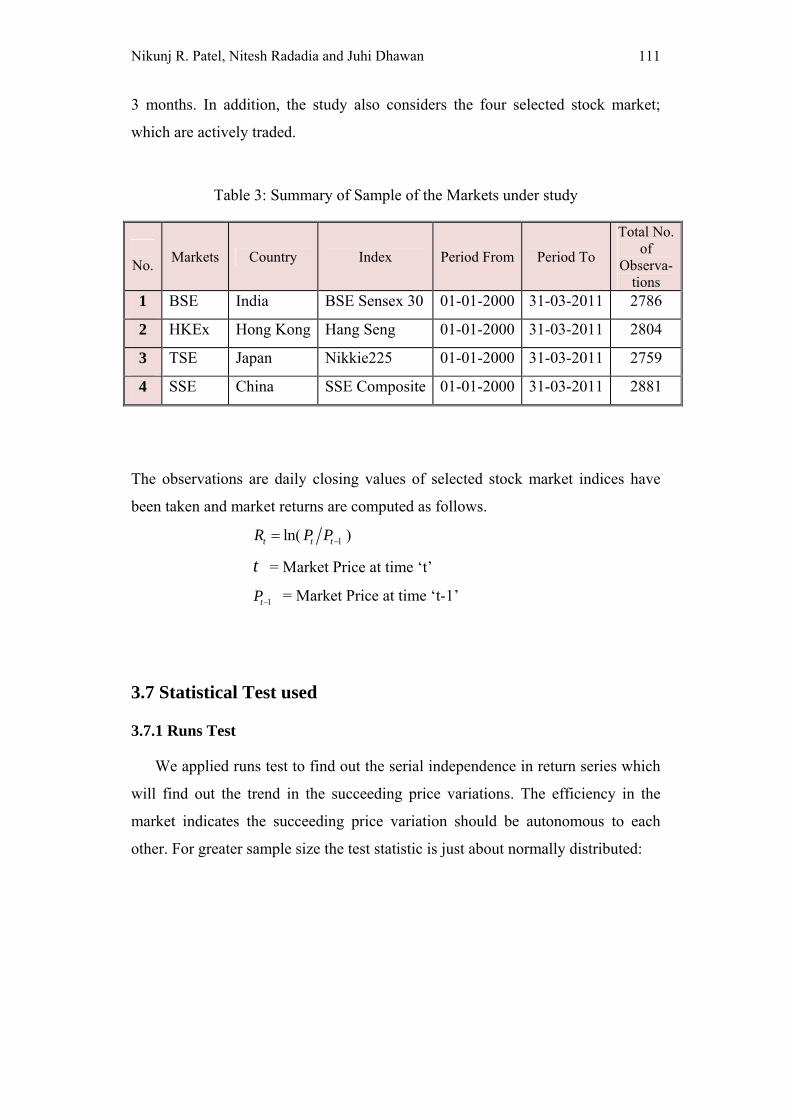
The Sample size varies from market to market. Following table 3 shows the

details of sample size in each market. The data are synchronized. The sample

includes observations of daily closing price of individual indices for 11 years and


3 months. In addition, the study also considers the four selected stock market;

which are actively traded.

Table 3: Summary of Sample of the Markets under study

No.

Markets Country Index Period From Period To

Total No. of

Observa- tions

1 BSE India BSE Sensex 30 01-01-2000 31-03-2011 2786

2 HKEx Hong Kong Hang Seng 01-01-2000 31-03-2011 2804

3 TSE Japan Nikkie225 01-01-2000 31-03-2011 2759

4 SSE China SSE Composite 01-01-2000 31-03-2011 2881

The observations are daily closing values of selected stock market indices have

been taken and market returns are computed as follows.

ln( )t t tR P P

t = Market Price at time ‘t’

tP = Market Price at time ‘t-1’

3.7 Statistical Test used

3.7.1 Runs Test

We applied runs test to find out the serial independence in return series which

will find out the trend in the succeeding price variations. The efficiency in the

market indicates the succeeding price variation should be autonomous to each

other. For greater sample size the test statistic is just about normally distributed:


where

2m m

m

, and

m m m m m

m m

3.7.2 Unit Root Tests

Augmented Dickey-Fuller (ADF) test is applied to assay the existence of unit

root in the time series of stock price return in the indices. Majorly it is used to test

the stationarity of the time series.

j

t 0 1 0 t 1 i it-1 tt=1

b bR R R

3.7.3 Kolmogorov-Smirnov (KS) Test

KS Test is a widely used goodness-of-fit test. It compares the observed

cumulative distribution function for a variable with a specified theoretical

distribution which may be normal, uniform, Poisson, or exponential. It checks

whether the observations have come from the specified distribution.

3.7.4 Auto Correlation

The autocorrelation test is used to test the relationship between the time

series and its own values at different lags. If the autocorrelation is negative it

means it is mean reversal and accepts the null hypothesis and if the result is

positive coefficients then it cannot accept the null hypothesis.

2

-1

( )( 2)

k

Ljung Boxt

tQ n n

n t


3.7.5 Variance Ratio Tests

A significance assumption of the random walk theory is investigated through

variance ratio test. If Rt is a random walk then the ratio of the variance of the jth

difference scaled by “J” to the Variance ( ) of the first difference have a

probability equal to one, that is why the Variance ( ) of the j-difference boosts

linearly in the surveillance interval,

( )

( )( )

jVR j

j

where,

th( )j j variance

(1) is the variance of the first differences

For that null hypothesis;

H0: VR (q) = 1 means Markets under the study are weak-form efficient

Ha: VR (q) ≠ 1 means Markets under the study are not Weak-form efficient

3.8 Expected Contribution of the Study

In our study, we intend to contribute to the empirical literature on tests of

Efficient Market Hypothesis by employing various statistical tests to investigate

weak form EMH for various exchanges of Asian countries using daily frequencies

of data set. A comparison of the results for Indian Stock Market with the results

for other countries’ share markets would provide additional understanding of the

relative market efficiency of Indian Stock Markets. We also propose to use

Chinese Stock Market data set to compare our results with them. The comparison

would provide gainful insight in understanding efficiencies in the stock markets.

The findings of this study will be useful to those involved in investment

decision-making in the stock market of India, as it will increase their

understanding of the pricing process prevailing in the stock market.


3.9 Scope for the Future Research

In our study, only the weak-form EMH is considered while the semi-strong

and Strong form EMH would be the concern of future research. Also, instead of

index returns, individual share price data of the markets might turn better results in

terms of market efficiency with weekly data or monthly data. For further research

sample of one country indexes can be taken and various tests can be applied to

know its impact on each other which is not applied in our research.

4 Data Analysis of Weak-Form Market Efficiency

4.1 Analysis of Descriptive Statistics

One of the assumptions of the random walk model is that the distribution of

the return series should be normal. In order to test the distribution of the series, the

descriptive statistics of the log of market returns are calculated and presented in

the below Table 4.

During the period from 1st Jan 2000 to 31st March 2011 BSE Sensex,

HANGSENG and SSE Composite markets showed positive average daily returns

except NIKKEI, the highest daily return came from the BSE Sensex (India) at

0.05% followed by SSE Composite 0.03% HANGSENG 0.01%. The lowest daily

return is witnessed by the 0.01%. At the same time BSE Sensex is showing 0.14%

median which is moving in positively and showing good sign for return whereas

NIKKEI did not indicate and shows 1.76% volatility which is less than the other

markets where BSE Sensex shows 1.88% volatility, SSE Composite at 1.82% and

HANGSENG at 1.80%. The markets can also be compared on the basis of

Average Daily Return to S.D. Ratio. The highest ratio indicates the best Risk

Return craving because this indicates average daily return per unit of S.D. The

BSE Sensex showed highest ratio of 2.79% followed by SSE COMPOSITE and


HANGSENG 1.68% and 0.74% when NIKKEI are on negative side at -0.74%.

Table 4: Results Descriptive Statistics for the selected Markets Returns

(Full Sample)

BSE SENSEX HANGSENG NIKKEI SSE

COMPOSITE

Mean 0.05% 0.01% -0.03% 0.03%

Median 0.14% 0.04% 0.00% 0.05%

Maximum 15.99% 16.80% 13.23% 9.03%

Minimum -11.81% -13.58% -12.92% -9.26%

Std. Dev. 1.88% 1.80% 1.76% 1.82%

Average daily Return

to S.D. Ratio 2.79% 0.74% -1.58% 1.68%

Skewness -0.101 0.307 -0.597 0.040

Kurtosis 9.245925 13.36848 10.70208 6.459555

Jarque-Bera 3910.14 10801.65 6082.465 1199.002

Probability 0.0000 0.0000 0.0000 0.0000

Sum 1.264489 0.320683 -0.6668 0.733345

Sum Sq. Dev. 0.850982 0.78199 0.741568 0.796129

No. of observation 2403 2403 2403 2403

The Values for Skewness 0 and kurtosis 3 represents that the observed

distribution is perfectly normally distributed. Here the value of skewness and

kurtosis of stock return series of the four selected Asian stock markets are not

equal to 0 and 3 respectively, which is (negative skewed for BSE Sensex -0.101

and NIKKEI -0.597 and Positive for HANGSENG 0.307 and SSE composite

0.040), and the value of all markets of Kurtosis is positive, thereby indicating

mesokurtic distribution. The evidence of negative skewness for returns series in

two markets BSE Sensex and NIKKEI indices returns are similar to findings of


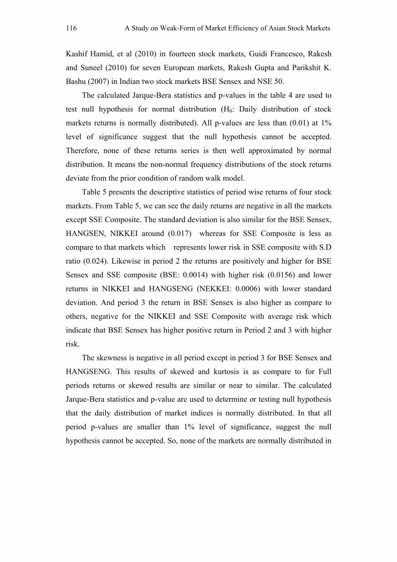
Kashif Hamid, et al (2010) in fourteen stock markets, Guidi Francesco, Rakesh

and Suneel (2010) for seven European markets, Rakesh Gupta and Parikshit K.

Bashu (2007) in Indian two stock markets BSE Sensex and NSE 50.

The calculated Jarque-Bera statistics and p-values in the table 4 are used to

test null hypothesis for normal distribution (H0: Daily distribution of stock

markets returns is normally distributed). All p-values are less than (0.01) at 1%

level of significance suggest that the null hypothesis cannot be accepted.

Therefore, none of these returns series is then well approximated by normal

distribution. It means the non-normal frequency distributions of the stock returns

deviate from the prior condition of random walk model.

Table 5 presents the descriptive statistics of period wise returns of four stock

markets. From Table 5, we can see the daily returns are negative in all the markets

except SSE Composite. The standard deviation is also similar for the BSE Sensex,

HANGSEN, NIKKEI around (0.017) whereas for SSE Composite is less as

compare to that markets which represents lower risk in SSE composite with S.D

ratio (0.024). Likewise in period 2 the returns are positively and higher for BSE

Sensex and SSE composite (BSE: 0.0014) with higher risk (0.0156) and lower

returns in NIKKEI and HANGSENG (NEKKEI: 0.0006) with lower standard

deviation. And period 3 the return in BSE Sensex is also higher as compare to

others, negative for the NIKKEI and SSE Composite with average risk which

indicate that BSE Sensex has higher positive return in Period 2 and 3 with higher

risk.

The skewness is negative in all period except in period 3 for BSE Sensex and

HANGSENG. This results of skewed and kurtosis is as compare to for Full

periods returns or skewed results are similar or near to similar. The calculated

Jarque-Bera statistics and p-value are used to determine or testing null hypothesis

that the daily distribution of market indices is normally distributed. In that all

period p-values are smaller than 1% level of significance, suggest the null

hypothesis cannot be accepted. So, none of the markets are normally distributed in


the period 1, 2 and 3. From this analysis we can say that the investment in the

period of 2 and 3 in BSE Sensex and HANGSENG is better because Average

daily returns to standard deviation ratio is positive and higher.

Table 5: Results Descriptive Statistics for the selected Markets Returns

(Period wise)

Sample: 05/01/2000 to 20/10/2003 Sample: 21/10/2003 to 29/06/2007

BSE

HANG

SENG

NIKKEI

SSE

BSE

HANG

SENG

NIKKEI

SSE

Mean -0.0002 -0.0004 -0.0007 0.0000 0.0014 0.0007 0.0006 0.0013

Median 0.0009 -0.0010 -0.0012 0.0001 0.0022 0.0009 0.0007 0.0012

Maximum 0.1046 0.0760 0.0722 0.0885 0.0793 0.0377 0.0677 0.0790

Minimum -0.0821 -0.1023 -0.0901 -0.0654 -0.1181 -0.0537 -0.0775 -0.0926

Std. Dev. 0.0175 0.0169 0.0172 0.0144 0.0156 0.0102 0.0122 0.0165

Avg. daily

returns to

S.D. Ratio

-0.0088 -0.0251 -0.0385 -0.0029 0.0882 0.0712 0.0498 0.0781

Skewness -0.1637 -0.1849 -0.0532 0.7127 -0.8606 -0.4737 -0.4018 -0.2099

Kurtosis 6.5061 6.8200 4.9156 9.5363 9.8569 5.7400 6.7471 6.7871

Jarque-Bera 413.85 491.58 122.85 1493.69 1668.1 280.54 490.16 484.54

Probability 0.000* 0.000* 0.000* 0.000* 0.000* 0.000* 0.000* 0.000*

Sum Sq.

Dev. 0.2457 0.2286 0.2374 0.1654 0.1958 0.0837 0.1183 0.2183

Observations 801 801 801 801 801 801 801 801

Sample: 03/07/2007 31/03/2011

BSE SENSEX HANGSENG NIKKEI SSE COMPOSITE

Mean 0.0004 0.0001 -0.0008 -0.0003

Median 0.0011 0.0007 -0.0001 0.0009

Maximum 0.1599 0.1680 0.1323 0.0903


Minimum -0.1160 -0.1358 -0.1292 -0.0804

Std. Dev. 0.0226 0.0242 0.0219 0.0227

Avg. daily returns to S.D.

Ratio 0.0156 0.0040 -0.0353 -0.0146

Skewness 0.2090 0.5047 -0.7645 -0.0042

Kurtosis 8.7873 10.5754 10.6680 4.6285

Jarque-Bera 1123.64 1949.29 2040.43 88.51

Probability 0.000* 0.000* 0.000* 0.000*

Sum Sq. Dev. 0.4086 0.4692 0.3849 0.4112

Observations 801 801 801 801

*indicate 1 % level of significance

4.2 Runs Test

Runs test is a non-parametric test that is designed to examine whether

successive price changes are independent. The non-parametric runs test is

applicable as a test of randomness for the sequence of returns. Accordingly, it tests

whether returns in emerging market indices are predictable. The null hypothesis

for this test is for temporal independence in the series (or weak-form efficiency):

in this perspective this hypothesis is tested by observation the number of runs or

the sequence of successive price changes with the same sign i.e. positive, zero or

negative. Each change in return is classified according to its position with respect

to the mean return. Hereby, it is a positive change when return is greater than the

mean, a negative change when the return is less than the mean and zero when the

return equals to the mean (Gupta, Rakesh and Maheshwari, 2010)). To perform

the runs test, the runs can be carried out by comparing the actual runs R to the

expected number of runs.


Table 6: Results of the Runs Test (Full Sample)

BSE SENSEX HANGSENG NIKKEI SSE

COMPOSITE

K=Mean .00052621 .00013345 -.00027749 .00030518

Cases < K 1127 1183 1186 1176

Cases >= K 1276 1220 1217 1227

Total Cases 2403 2403 2403 2403

Number of Runs 1128 1206 1264 1206

Z- Statistic -2.863 0.154 2.518 0.165

p-value 0.004* 0.877 0.012** 0.869

Notes: if the Z-statistic is greater than or equal to ± 1.96, then we cannot be accepted null hypothesis at 5% level of significance.

* Indicates non acceptance of the null hypothesis that successive price changes are

independent. * indicate 1 % level of significance,

**indicate 5 % level of significance

As pointed out by Guidi, Rakesh and Maheshwari (2010), when actual

number of runs exceed (fall below) the expected runs, a positive (negative) Z

values is obtained. A negative Z value indicates a positive serial correlation,

whereas a positive Z value indicates a negative serial correlation. The positive

serial correlation implies that there is a positive dependence of stock prices,

therefore indicating a violation of random walk. Since the distribution Z is N (0,1),

the critical value of Z at the five percent significance level is ±1.96 .

The results of Runs test for the returns on markets under the study are

indicating in the above table 6. For the full period, the runs test clearly shows that

the successive returns for all indices except the HANGSENG and SSE composite,

are not independent at 1% and 5% level of significance (significance value of

±1.96) and the null hypothesis of return independence because our p-value is less


than 0.05 at 5% level of significance.(H0: The succeeding price changes are not

dependent and move randomly) which indicate null hypothesis cannot be accepted

in BSE Sensex and NIKKEI which indicated that both markets are inefficient,

means not weak form efficient for whole period so investor can predict the

markets returns. This result for the full sample period is consistent with Rakesh

Gupta and Parikshit K. Basu (2007). And HANGSENG and SSE Composite, we

cannot reject null hypothesis, concluded that both markets are efficient and follow

random walk so investor cannot predicted the market returns for whole period.

From the Table 7 indicate period wise analysis in three interval period, In the

first period we can interpret that the markets under the study shows Weak-Form

efficiency except BSE Sensex in all three period. All the estimated Z-values are

insignificance at the 1% and 5% level of significance except BSE Sensex which

indicates inefficiency on period-1 in BSE Sensex and p-value is significance at 5%

level of significance, the null hypothesis the succeeding price changes are not

dependent and move randomly cannot be accepted. Where in other three markets,

HANGSENG, NIKKEI and SSE Composite our null hypothesis accepted which

indicate markets are efficient in weak-form.

The results of Runs test of the second period on the markets under the study

are reported in above table. For that period, the runs test clearly shows that

markets under the study are Weak-Form efficient and so the null hypothesis of the

return independence is accepted in second period which indicate means the

markets under the study follow random walk and so we cannot predict the

behavior markets returns during second interval period.

And the above table for the third period null hypothesis accepted at 5% level

of significance elucidates that succeeding price changes are not dependent and

follow random walk. So we can conclude that a return of markets under the study

is clearly shows Weak-Form efficient and not easily predictable. This finding is

also similar of Kashif Hamid et al (2010).


Table 7: Results of the Runs Test (Period wise)

Sample:05/01/2000 to 20/10/2003

Mean= k Cases < K Cases >= K

Total

Cases

Number

of Runs Z-statistic p-value

BSE -0.0002 375 426 801 365 -2.476 0.013**

HANGSENG -0.0004 418 383 801 398 -0.194 0.846

NIKKEI -0.0007 413 388 801 398 -0.220 0.826

SSE 0.0000 395 406 801 394 -0.525 0.600

Sample: 21/10/2003 to 29/06/2007

BSE 0.0014 372 429 801 386 -0.957 0.338

HANGSENG 0.0007 390 411 801 420 1.329 0.184

NIKKEI 0.0006 397 404 801 426 1.735 0.083***

SSE 0.0013 401 400 801 390 -0.813 0.416

Sample: 03/7/2007 to 31/3/2011

BSE 0.0004 383 418 801 395 -0.406 0.685

HANGSENG 0.0001 394 407 801 395 -0.452 0.651

NIKKEI -0.0008 380 421 801 427 1.882 0.060***

SSE -0.0003 382 419 801 408 0.521 0.602

Notes: if the Z-statistic is greater than or equal to ± 1.96, then we cannot be accepted null hypothesis at 5% level of significance.

* Indicates rejection of the null hypothesis that successive price changes are independent. * Indicates 1% level of Significance

** Indicates 5% level of Significance

*** Indicates 10 % level of Significance

4.3 Unit Root Test

Since unit root is necessary condition for a random walk, the Augmented

Dickey-Fuller test is used to test the null hypothesis of a unit root. The results of

Augmented Dickey-Fuller for the unit root of all the markets under study are


presented in the following Table 8. ADF unit root was performed for the whole

sample period Jan 2000 to March 2011 for the maximum lag period of 36.

Table 8: Results of Augmented Dickey-fuller for the markets under study

(Full Sample).

BSE SSE

SENSEX HANGSENG NIKKEI COMPOSITE

ADF -46.6777 -48.5725 -48.5901 -48.5967

p-value 0.0001* 0.0001* 0.0001* 0.0001*

*indicate 1% level of significance

The t- statistics critical value at 1%, 5% and 10% are -3.43288, -2.86254, and

-2.56735 respectively and it clearly showed stationary because the null hypothesis

of unit root (H0: Series contains a unit root) is convincingly cannot be accepted,

suggesting that these market show the existence of random walk which is similar

to the findings of Rakesh Gupta and Parikshit K. Basu (2007).

The Table 9 presents the unit root test analysis in different intervals e.g.,

Sample: 05/01/2000 to 20/10/2003, Sample: 10/21/2003 6/29/2007, Sample:

7/03/2007 3/31/2011. In above table the t-statistics at 1%, 5% and 10 % are

-3.4383, -2.86494 and -2.568634 respectively and it clearly showed stationery in

all sub period as the p-value<0.05 which does not accept null hypothesis (H0:

Series contains unit root). Therefore null hypothesis cannot be accepted at 1%, 2%

and 10% level of significance which shows that series is stationery. The results

therefore indicate that there exists of some evidences of random walk in all the

selected Stock markets for that periods.

Unit root test alone cannot be used to conclude that markets under study are

weak form efficient as it does not detect the predictability of return. So there is a

need to apply other tests as well.


Table 9: Results of the Augmented Dickey-Fuller and Unit Root Test for the

selected markets (Period wise)

Sample:05/01/2000 to 20/10/2003

BSE

SENSEX HANGSENG NIKKIE

SSE

COMPOSITE

ADF -26.3982 -27.5017 -28.7646 -27.4932

p-value 0.0000* 0.0000* 0.0000* 0.0000*

Sample: 10/21/2003 6/29/2007

BSE


SSE

COMPOSITE

ADF -27.1059 -27.8532 -28.8502 -28.6794

p-value 0.0000* 0.0000* 0.0000* 0.0000*

Sample: 7/03/2007 3/31/2011

BSE


SSE

COMPOSITE

ADF -27.2349 -28.3174 -27.3743 -27.9313

p-value 0.0000* 0.0000* 0.0000* 0.0000*


4.4 Kolmogorov-Smirnov Test:

The non-parametric, Kolmogorov Smirnov Goodness of Fitness Test (KS) test

whether the observed distribution fit theoretical normal or uniform distribution.

Kolmogorov Smirnov Goodness of Fitness Test (KS) is used to determine how

well a random sample of data fits a particular distribution (uniform, normal,

poisson). It is based on comparison of the sample’s cumulative distribution against

the standard cumulative function for each distribution. The Kolmogorov- Smirnov


one sample goodness of fit test compares the cumulative distribution function for a

variable with a uniform or normal distributions and tests whether the distributions

are homogeneous. We use both normal and uniform parameters to test

distribution.

Table 10: Results of K-S Goodness of fit test (Full Sample: Normal Distribution)

Absolute Positive Negative K-S-Z P-value

BSE SENSEX 0.076 0.074 -0.076 3.736 0.000*

HANGSENG 0.083 0.077 -0.083 4.048 0.000*

NIKKEI 0.061 0.049 -0.061 3.007 0.000*

SSE COMPOSITE 0.075 0.07 -0.075 3.673 0.000*


The Kolmogorov Smirnov Goodness of Fit Test (KS) shows p-value < 0.05

at the 1%, 5% and 10% level of significance, in case of normal distribution. The

results clearly indicate that the frequency distribution of the daily values of the

markets under the study does not fit normal distribution. The above table 10

indicates the null hypothesis cannot be accepted which means the all markets

under the study does not follow normal distributed because it provide p-value

which is insignificance at the 1% level of significance the evidence of all the

markets under study are similar to findings of Sunil Poshakwale (1996) of Indian

stock markets, Rengasamy Elango, and Mohammed Ibrahim Hussein(1996) of

GGC markets. (Significance at 0.05) these results are also similar finding with

descriptive statistics which also indicate markets under the study does not follow

normal distribution. (H0: The stock returns of the markets under the study follow

normal distribution).


Table 11: Results of K-S Goodness of fit test (Period wise)

Period:05/01/2000 to 20/10/2003


BSE SENSEX 0.062 0.054 -0.062 1.759 0.004*

HANGSENG 0.052 0.052 -0.052 1.479 0.025**

NIKKEI 0.029 0.029 -0.026 0.814 0.521

SSE COMPOSITE 0.09 0.09 -0.075 2.543 0.000*

Sample: 10/21/2003 6/29/2007


BSE SENSEX 0.086 0.075 -0.086 2.427 0.000*

HANGSENG 0.072 0.048 -0.072 2.032 0.001*

NIKKEI 0.057 0.038 -0.057 1.626 0.010**

SSE COMPOSITE 0.059 0.059 -0.057 1.669 0.008*

Sample: 7/03/2007 3/31/2011


BSE SENSEX 0.079 0.079 -0.075 2.239 0.000*

HANGSENG 0.082 0.082 -0.077 2.332 0.000*

NIKKEI 0.078 0.062 -0.078 2.195 0.000*

SSE COMPOSITE 0.076 0.058 -0.076 2.161 0.000*


**indicate 5% level of significance

From the above Table 11 analyze daily returns of the markets under the study in

different period i.e. Period: 05/01/2000 to 20/10/2003, Sample: 10/21/2003

6/29/2007 and Sample: 7/03/2007 3/31/2011. In the first period, concluded that at

1%, 5% and 10% level of significance all the markets under the study follow

normal distribution except NIKKEI in the period 1 as compared to whole period,

null hypothesis cannot be accepted in the BSE Sensex, HANGSENG and SSE

Composite it means those markets returns are not follow normal distribution.


Where NIKKEI indices null hypothesis can be accept at 10% level of significance.

The second interval period indicate from the table 11 that all the markets

under the study shows patterns of normal distribution as compared to whole period

and period one, we can conclude that at 1%, 5% and 10% level of significance all

the markets under the study follow normal distribution, null hypothesis cannot be

accepted in the BSE Sensex, HANGSENG, NIKKEI and SSE Composite it shows

that the markets returns are not follow normal distribution. And for the third

period interval, concluded that at 1%, 5% and 10% level of significance all the

markets under the study follow normal distribution, null hypothesis cannot be

accepted in the BSE Sensex, HANGSENG, NIKKEI and SSE Composite it shows

that the markets returns are not follow normal distribution.

4.5 Auto-Correlation Test

Our literatures provide evidence that Auto-correlation test used to test weak

form market efficiency. Auto-correlation test is a reliable measure for testing of

either dependence or independence of random variables in a series. Kendall (1948,

p. 412) compute the price changes at different lagged 1,2,3,4 time periods. Later

the test is used very popularly (e.g., Laurence, 1986; Claessens, Dasgupta and

Glen, 1995; Poshokwale, S. 1996; Nicolas, 1997; Nourredine Khaba, 1998). The

serial correlation coefficient measures the relationship between the values of a

random variable at time t and its value in the previous period. Auto correlation test

evidences whether the correlation coefficients are significantly different from zero.

The auto-correlation coefficients have been computed for the log of the market

return series that shows significant auto-correlation at different lags for the whole

sample period.

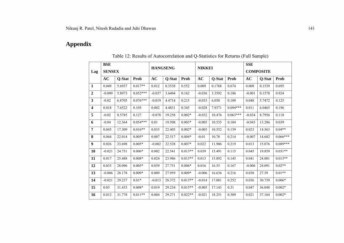
In Appendix, Table 12 provides the results of the sample autocorrelation

coefficients and the Ljung-box statistics for the daily returns on the indices for


BSE Sensex, HANGSENG, NIKKEI and SSE composite markets for the full

sample period 5/1/2000- 31/03/2011. To test the Random walk hypothesis for the

selected markets under study, autocorrelation tests up to 36 lags were performed

for daily stock returns.

Positive autocorrelation indicates predictability of returns in short period,

which is general evidence against market efficiency, whereas negative

autocorrelation indicate mean reversion in returns. BSE Sensex appears the

significant negative correlation at lag 2, 3, 5, 6, 10, 13, 14, 17, 18, 20, 22, 23, 24,

29, 32 and 34. HANGSENG also shows significant negative autocorrelation at lag

2, 3, 5, 9, 14, 17, 18, 20, 23, 25, 29, 31, 32and 36. Nikkei shows negative

autocorrelation at lag 2 to 8, 13 to 16, 18 to 20, 24, 28 to 31. And SSE composite

shows negative autocorrelation at lag 2, 5, 6, 8, 12, 17 to 23, 26, 29, 30, 34. Thus,

it shows that at the above lags the returns cannot be predicted and weak form of

efficiency holds.

Ljunj-Box statistics also provide evidence of possible dependence. The

Ljunj- Box Q- statistics shows that the null hypothesis is of no autocorrelation (H0:

There is no autocorrelation) if p-value is significant at 1 % and 5% (p-value<0.05).

So in BSE the null hypothesis cannot be accepted for all lags except lag 2 to 6 and

34 to 36. It means that returns are auto correlated from lag 2 to6 and 34 to 36 in

BSE Sensex. Similarly the returns are not auto correlated in the HANGSENG

except for lag 1 to 4. The returns for Nikkei market are not auto correlated except

for lag 1 to 20.And the returns of SSE composite are not auto correlated except for

lag 1 to 5 and 8, 9.

According to Auto correlation test it is inferred that the equity markets of the

Asian region under the study remained inefficient for some period whereas they

were efficient for the other period. After whole discussion it is worth nothing that

the acceptance or rejection of the null hypothesis does not entails that the equity

markets are efficient or inefficient respectively, because of conclusion of this

research are based on samples.


Table 13: Results of Auto-correlation test and Q-Statistics for Returns (Period wise)

Sample:

05/01/2000 to 20/10/2003

Sample:

21/10/2003 to 29/06/2007

Sample:

30/07/2007 to 31/03/2011

BSE

HANG

SENG NIKKEI SSE BSE

HANG

SENG NIKKEI SSE BSE

HANG

SENG NIKKEI SSE

p1 0.068 0.039 -0.017 0.027 0.042 0.014 -0.021 -0.017 0.037 -0.002 0.031 0.012

p2 0.026 -0.037 -0.007 0.002 -0.081 -0.028 -0.023 0.021 0.002 -0.040 -0.061 -0.016

p3 -0.037 0.049 -0.002 -0.069 -0.001 -0.038 -0.006 0.078 -0.022 -0.048 -0.062 0.070

p4 0.039 -0.004 -0.037 0.031 0.067 0.031 -0.076 0.015 -0.018 -0.001 -0.009 -0.003

p5 -0.004 -0.089 0.033 0.029 0.041 0.015 0.065 -0.029 -0.061 -0.091 -0.104 -0.053

p6 -0.037 0.007 -0.046 -0.031 -0.112 -0.041 -0.041 -0.030 -0.008 0.021 0.029 -0.058

p7 0.035 -0.001 -0.002 -0.012 -0.007 -0.009 -0.034 -0.008 0.075 0.057 0.007 0.038

p8 0.059 0.011 -0.020 -0.016 0.024 -0.087 -0.051 -0.007 0.045 0.021 0.011 -0.004

p9 0.020 0.035 -0.019 -0.007 0.079 0.048 -0.014 0.036 0.003 -0.032 0.054 0.012

p10 -0.006 0.031 0.026 0.042 -0.046 -0.004 0.039 0.063 -0.017 -0.008 0.046 0.031

p11 -0.004 0.019 -0.029 0.062 -0.081 0.036 0.030 0.047 0.073 0.023 0.030 0.033

p12 -0.012 -0.001 0.047 -0.002 0.032 -0.016 -0.002 -0.024 0.056 0.066 -0.003 -0.002

p13 0.000 -0.020 -0.053 -0.029 0.015 -0.001 -0.027 0.123 -0.021 0.020 0.026 0.016

p14 -0.069 -0.008 0.005 0.043 0.033 0.004 0.027 0.007 -0.024 -0.021 -0.044 0.055

p15 0.014 0.019 0.018 0.030 -0.006 0.033 0.011 0.136 0.055 0.020 -0.029 0.005

p16 0.017 0.008 -0.014 0.054 0.050 0.001 0.008 -0.060 -0.020 -0.001 -0.040 0.043

p17 -0.003 -0.004 -0.002 -0.040 -0.010 -0.035 0.027 0.006 -0.004 -0.004 0.048 0.000


p18 -0.113 -0.016 -0.002 0.001 0.003 -0.061 -0.010 -0.014 -0.021 0.008 -0.049 -0.019

p19 -0.035 0.011 -0.033 -0.018 -0.031 -0.019 -0.004 -0.062 0.043 0.052 -0.024 0.025

p20 0.050 0.032 -0.011 0.018 -0.045 -0.026 -0.013 0.009 -0.032 -0.071 -0.091 -0.022

p21 0.022 0.001 -0.007 -0.070 -0.015 -0.017 -0.035 -0.035 0.061 0.051 0.104 0.003

p22 0.001 -0.013 -0.010 -0.004 -0.055 -0.052 0.009 -0.014 -0.016 0.020 0.030 -0.013

p23 -0.006 0.025 0.080 -0.067 0.054 -0.059 -0.038 0.061 -0.028 -0.029 0.025 -0.048

p24 -0.019 -0.026 -0.010 0.036 -0.073 0.014 0.029 0.095 -0.037 0.022 -0.050 0.021

p25 -0.001 -0.054 0.046 -0.009 -0.039 0.022 -0.038 -0.018 0.081 -0.038 0.000 0.034

p26 -0.051 0.009 0.010 -0.021 0.007 0.026 -0.014 0.022 0.034 0.020 0.063 -0.075

p27 -0.029 0.008 -0.009 -0.011 0.030 0.035 0.051 0.020 0.034 0.021 -0.010 0.037

p28 0.001 0.051 -0.018 -0.006 0.007 0.030 -0.021 0.110 0.003 -0.002 -0.007 0.081

p29 0.000 -0.007 -0.026 -0.010 -0.047 -0.011 0.017 -0.040 0.010 -0.039 -0.019 -0.051

p30 0.022 0.006 -0.004 -0.015 0.040 0.005 0.018 0.012 -0.018 -0.003 -0.010 -0.011

p31 0.035 -0.112 -0.048 0.023 0.022 -0.038 -0.032 0.016 0.000 -0.021 -0.028 0.062

p32 -0.046 -0.034 0.002 0.020 -0.010 -0.026 0.072 0.006 -0.018 -0.070 -0.016 0.003

p33 -0.044 -0.042 0.029 -0.032 0.003 -0.033 0.033 0.030 0.038 0.065 0.002 0.008

p34 -0.038 -0.015 0.053 -0.031 -0.083 -0.041 -0.062 0.016 0.014 0.025 0.049 -0.022

p35 0.000 -0.042 0.002 0.035 0.033 0.003 -0.105 -0.011 -0.011 0.089 0.061 0.090

p36 0.052 0.003 -0.016 0.036 0.038 0.022 0.067 -0.012 -0.030 -0.015 0.016 0.034


Sample:05/01/2000 to 20/10/2003 Sample:21/10/2003 to 29/06/2007 Sample:30/07/2007 to 31/03/2011

BSE HANG

SENG NIKKEI SSE BSE

HANG

SENG NIKKEI SSE BSE

HANG

SENG NIKKEI SSE

(Q)1 3.750 1.210 0.237 0.583 1.435 0.158 0.351 0.220 1.077 0.004 0.793 0.111

p-value 0.053*** 0.271 0.626 0.445 0.231 0.691 0.554 0.639 0.299 0.952 0.373 0.739

(Q)2 4.293 2.289 0.281 0.587 6.760 0.788 0.775 0.566 1.079 1.298 3.746 0.324

p-value 0.117 0.318 0.869 0.745 0.034** 0.674 0.679 0.753 0.583 0.523 0.154 0.851

(Q)3 5.394 4.189 0.284 4.381 6.760 1.962 0.809 5.444 1.468 3.152 6.847 4.238

p-value 0.145 0.242 0.963 0.223 0.080*** 0.580 0.847 0.142 0.690 0.369 0.077** 0.237

(Q)4 6.596 4.204 1.411 5.174 10.378 2.735 5.517 5.623 1.733 3.152 6.919 4.245

p-value 0.159 0.379 0.842 0.270 0.035** 0.603 0.238 0.229 0.785 0.533 0.140 0.374

(Q)5 6.611 10.632 2.285 5.875 11.711 2.917 8.936 6.307 4.729 9.798 15.661 6.537

p-value 0.251 0.059*** 0.809 0.319 0.039** 0.713 0.112 0.278 0.450 0.081** 0.008* 0.257

(Q)6 7.718 10.666 4.016 6.659 21.800 4.308 10.299 7.030 4.777 10.145 16.333 9.252

p-value 0.260 0.099*** 0.675 0.354 0.001* 0.635 0.113 0.318 0.573 0.119 0.012** 0.160

(Q)7 8.686 10.667 4.020 6.767 21.840 4.374 11.226 7.080 9.338 12.822 16.371 10.395

p-value 0.276 0.154 0.777 0.454 0.003* 0.736 0.129 0.421 0.229 0.077*** 0.022** 0.167

(Q)8 11.502 10.770 4.351 6.984 22.322 10.492 13.345 7.119 10.961 13.180 16.468 10.410

p-value 0.175 0.215 0.824 0.538 0.004* 0.232 0.101 0.524 0.204 0.106 0.036** 0.237

(Q)9 11.840 11.765 4.639 7.028 27.392 12.396 13.507 8.144 10.970 14.002 18.876 10.522


p-value 0.222 0.227 0.865 0.634 0.001* 0.192 0.141 0.520 0.278 0.122 0.026** 0.310

(Q)10 11.872 12.522 5.170 8.476 29.098 12.412 14.737 11.405 11.216 14.057 20.591 11.290

p-value 0.294 0.252 0.880 0.582 0.001* 0.258 0.142 0.327 0.341 0.170 0.024** 0.335

(Q)11 11.888 12.824 5.871 11.648 34.465 13.440 15.486 13.188 15.537 14.477 21.318 12.156

p-value 0.372 0.305 0.882 0.391 0.000* 0.266 0.161 0.281 0.159 0.208 0.030** 0.352

(Q)12 12.001 12.825 7.677 11.651 35.297 13.648 15.491 13.654 18.062 18.076 21.326 12.158

p-value 0.446 0.382 0.810 0.474 0.000* 0.324 0.216 0.323 0.114 0.113 0.046** 0.433

(Q)13 12.001 13.146 9.972 12.344 35.489 13.648 16.072 26.074 18.430 18.389 21.894 12.371

p-value 0.528 0.437 0.696 0.500 0.001* 0.399 0.245 0.017** 0.142 0.143 0.057*** 0.497

(Q)14 15.947 13.196 9.992 13.884 36.387 13.659 16.680 26.110 18.882 18.762 23.445 14.870

p-value 0.317 0.511 0.763 0.458 0.001* 0.475 0.274 0.025** 0.170 0.174 0.053*** 0.387

(Q)15 16.114 13.496 10.261 14.610 36.413 14.557 16.776 41.340 21.400 19.098 24.125 14.890

p-value 0.374 0.564 0.803 0.480 0.002* 0.484 0.332 0.000* 0.125 0.209 0.063*** 0.459

(Q)16 16.356 13.555 10.422 16.965 38.433 14.557 16.834 44.257 21.736 19.099 25.436 16.403

p-value 0.428 0.632 0.844 0.388 0.001* 0.557 0.396 0.000* 0.152 0.264 0.062*** 0.425

(Q)17 16.365 13.568 10.425 18.287 38.514 15.535 17.424 44.289 21.750 19.111 27.353 16.403

p-value 0.498 0.697 0.885 0.371 0.002* 0.557 0.426 0.000* 0.195 0.322 0.053*** 0.495

(Q)18 26.867 13.785 10.429 18.288 38.519 18.619 17.510 44.461 22.100 19.164 29.291 16.700

p-value 0.082*** 0.743 0.917 0.437 0.003* 0.416 0.488 0.000* 0.228 0.382 0.045** 0.544

(Q)19 27.848 13.887 11.339 18.564 39.289 18.909 17.523 47.638 23.652 21.418 29.747 17.227

p-value 0.086*** 0.790 0.912 0.485 0.004* 0.463 0.554 0.000* 0.210 0.314 0.055*** 0.574


Sample:05/01/2000 to 20/10/2003 Sample:21/10/2003 to 29/06/2007 Sample:30/07/2007 to 31/03/2011

BSE HANG

SENG NIKKEI SSE BSE

HANG

SENG NIKKEI SSE BSE

HANG

SENG NIKKEI SSE

(Q)20 29.879 14.713 11.437 18.823 40.983 19.454 17.655 47.711 24.480 25.548 36.636 17.630

p-value 0.072 0.793 0.934 0.533 0.004* 0.493 0.610 0.000* 0.222 0.181 0.013** 0.612

(Q)21 30.281 14.714 11.474 22.903 41.176 19.682 18.645 48.695 27.534 27.731 45.623 17.636

p-value 0.086*** 0.837 0.953 0.349 0.005* 0.541 0.608 0.001* 0.154 0.148 0.001* 0.672

(Q)22 30.282 14.850 11.564 22.913 43.645 21.901 18.710 48.860 27.750 28.077 46.378 17.770

p-value 0.112 0.869 0.966 0.407 0.004* 0.466 0.663 0.001* 0.184 0.173 0.002* 0.720

(Q)23 30.316 15.348 16.846 26.608 46.062 24.754 19.889 51.887 28.408 28.793 46.908 19.712

p-value 0.141 0.882 0.817 0.273 0.003* 0.363 0.649 0.001* 0.201 0.187 0.002* 0.659

(Q)24 30.622 15.926 16.924 27.670 50.512 24.915 20.598 59.306 29.571 29.192 48.958 20.088

p-value 0.165 0.891 0.852 0.274 0.001* 0.410 0.662 0.000* 0.199 0.213 0.002* 0.692

(Q)25 30.622 18.378 18.642 27.739 51.776 25.304 21.815 59.572 35.068 30.365 48.958 21.038

p-value 0.202 0.826 0.814 0.320 0.001* 0.445 0.646 0.000* 0.087*** 0.211 0.003* 0.690

(Q)26 32.818 18.447 18.732 28.091 51.817 25.871 21.966 59.992 36.009 30.689 52.273 25.653

p-value 0.167 0.859 0.848 0.354 0.002* 0.470 0.691 0.000* 0.092** 0.240 0.002* 0.482

(Q)27 33.505 18.501 18.793 28.190 52.554 26.892 24.149 60.320 36.966 31.061 52.361 26.770

p-value 0.181 0.887 0.877 0.401 0.002* 0.470 0.622 0.000* 0.096*** 0.269 0.002* 0.476

(Q)28 33.506 20.667 19.064 28.220 52.594 27.663 24.511 70.397 36.972 31.064 52.400 32.260


p-value 0.218 0.839 0.896 0.453 0.003* 0.482 0.654 0.000* 0.119 0.314 0.003* 0.264

(Q)29 33.506 20.707 19.613 28.308 54.399 27.772 24.754 71.716 37.049 32.308 52.712 34.403

p-value 0.258 0.870 0.905 0.501 0.003* 0.530 0.691 0.000* 0.145 0.307 0.005* 0.225

(Q)30 33.920 20.740 19.626 28.489 55.705 27.796 25.014 71.829 37.326 32.317 52.792 34.495

p-value 0.284 0.896 0.926 0.545 0.003* 0.581 0.724 0.000* 0.168 0.353 0.006* 0.261

(Q)31 34.943 31.160 21.586 28.934 56.123 29.016 25.844 72.054 37.326 32.668 53.445 37.702

p-value 0.286 0.458 0.896 0.573 0.004* 0.568 0.729 0.000* 0.201 0.385 0.007* 0.189

(Q)32 36.737 32.119 21.589 29.273 56.205 29.576 30.178 72.088 37.590 36.755 53.663 37.711

p-value 0.259 0.461 0.918 0.605 0.005* 0.590 0.559 0.000* 0.228 0.258 0.010* 0.224

(Q)33 38.348 33.571 22.308 30.112 56.211 30.464 31.115 72.827 38.782 40.291 53.666 37.768

p-value 0.240 0.440 0.921 0.612 0.007* 0.594 0.561 0.000* 0.225 0.179 0.013** 0.260

(Q)34 39.527 33.748 24.641 30.937 61.963 31.853 34.355 73.034 38.937 40.828 55.670 38.180

p-value 0.237 0.480 0.880 0.619 0.002* 0.573 0.451 0.000* 0.257 0.195 0.011** 0.285

(Q)35 39.527 35.239 24.644 31.980 62.880 31.862 43.642 73.130 39.031 47.479 58.756 45.000

p-value 0.275 0.457 0.904 0.615 0.003* 0.620 0.150 0.000* 0.293 0.078** 0.007* 0.120

(Q)36 41.762 35.246 24.858 33.049 64.089 32.284 47.460 73.243 39.792 47.676 58.979 45.949

p-value 0.235 0.504 0.919 0.610 0.003* 0.646 0.096 0.000* 0.305 0.092** 0.009* 0.124

*Significant at 1 % level

**Significant at 5% level

***Significant at 10% level


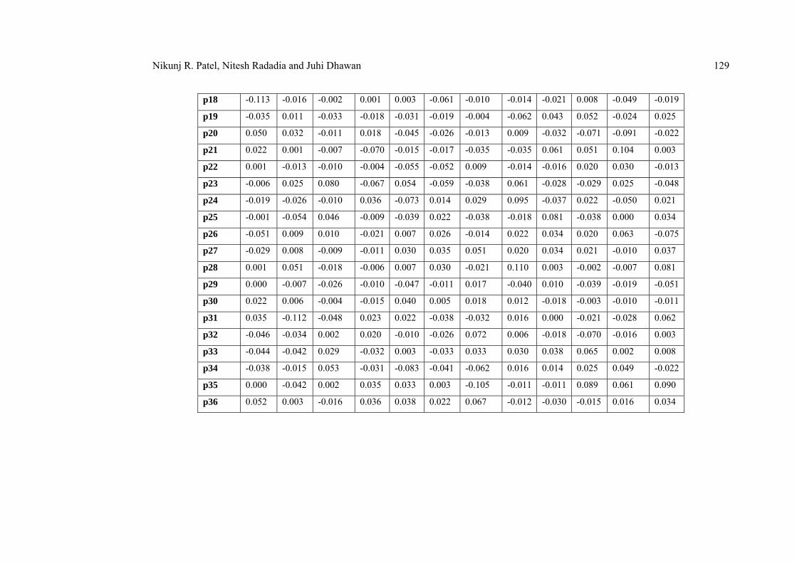
Table 13 provides the results of the sample autocorrelation coefficients and

the Lung- box statistics for the daily returns for the daily returns for 3 periods of

BSE Sensex, HANGSENG Nikkei and SSE composite. Table 13 provides the

results for Auto-correlation and Ljung- Box Q- statistic test for the 3 sub periods

i.e. 5th January 2000 to 20th October 2003, 21st October 2003 to 29th June 2007 and

3rd July 2007 to 31st March 2011. In the period of January 2000 to October 2003

returns did not have autocorrelation at 5% level of significance for all the markets

under study. It means the returns in 1st period are not auto correlated which shows

that market holds weak form of market efficiency.

In the period October 2003 to June 2007 returns on all the 4 markets show

the significance auto correlation at all the lags except lag 1 and 3 in BSE Sensex at

5 % level of significance. For HANGSENG and Nikkei returns do not have auto

correlation at 5 % level of significance. For SSE composite returns show

significant auto correlation for lags 1 to 12 only at 5 % level of significance.

In 3rd period from June 2007 to July 2007 BSE Sensex, HANGSENG, SSE

market shows no sign of autocorrelation at any lags. The null hypothesis is

accepted at 5 % significance level in BSE Sensex, HANGSENG, and SSE market

which shows that the returns are not auto correlated. But for Nikkei the null

hypothesis is rejected at 5 % level at lag 5 to 12, 18 and 20 to 36. It shows that the

returns are auto correlated at lag5 to 12, 18 and 20 to 36 which indicates that it

does not hold weak form of market efficiency.

4.6 Variance Ratio Test

Variance Ratio test introduced by Lo and Mackinlay (1988) is most

commonly used as a tool for investigate for randomness. When the random walk

hypothesis is rejected and VR (q) > 1, returns are positively serially correlated for

emerging markets positive serial correlation in returns could simply describe

market growth. When the random walk hypothesis is rejected and VR (q) < 1,


returns are negatively serially correlated. The situation is often described as a

mean reverting process and consistent. Under null hypothesis the variance ratio

should be approximately equal to 1. If the value is not equal to one then it means

that the series is auto correlated in first-order and the variance ratio is sum of

first-order autocorrelation coefficient estimator and unit value pointed by Bhanu

Pant and T. R. Bishnoi as per our literature.

From Table 14 in Appendix, we can interpret that the standardized VR (J)test

statistics for z (j) and p value is significant from J = 2 to J=16 for all markets

BSE Sensex ,HANGSENG,NIKKEI and SSE Composite (as p value is less than

0.05). An important observation in the above cases is that ,as variance ratio

increases with j, the z(j) also increase in all cases which indicates that as ‘j’

increases, the significance of rejection become stronger pointed out by Kashif

Hamid et al. (2010).

Our results of Variance ratio test are indicate similarity of previous findings

in emergence markets, e.g. Guidi, Rakesh and Maheseshwari (2010), Kashif

Hamidet al (2010), Mohammed Omran and Suzanne V. Farrar (2006).They find

that the markets are inefficient during the study so it can easily predicted.

According to Variance ratio test for our study is inferred that the market of Asian

region under the study remains in inefficient for the period 2000 to 2011.

Therefore our null hypothesis cannot be accepted which indicated that markets

does not follow Random Walk. (H0: VR (q) = 1).

In Appendix, Table 15 presents the results of the Variance Ratio test for the

daily returns for three periods of BSE Sensex, HANGSENG, NIKKEI and SSE

Composites. Here VR (j) is the variance at leg j, z (1) to z(16) are represents

z-statistics values and p-values are provide to test null hypothesis of VR (q) = 1 to

know the return series follow random walk. Table provides the results of the

variance and z statistics for the sub period i.e., Sample: 05/01/2000 to 20/10/2003,

Sample: 21/10/2003 to 29/06/2007, Sample: 03/07/2007 to 31/3/2011. In the first

period, The standardize Variance Ratio and test statistics for z(j) is significance at


j 2 to 16 for all markets and so that he returns series did not follow random walk in

the markets under the study, because here our null hypothesis cannot be accepted

at 1% level of significance (p-values is less than 0.05) in all legs from 2 to 16.In

the period 2, null hypothesis cannot be accepted at 1% level of significance all

p-values of daily returns series is not significance( p-values <0.05, significance)

and indicates the series did not follow random walk at none of the leg in

observation likewise happened in period 3, also null hypothesis cannot be

accepted and series of daily returns are not random walk. According to variance

ratio test it is inferred that the equity markets of the Asian region under the study

remained inefficient for the all period intervals and so investor can easily predict

market behavior and take benefit of profit.

4.7 Major Findings of the Study

Our study investigates the weak form of market efficiency in the selected

markets of Asia. The sample size consisted of 4 equity markets with their daily

closing returns. The purpose of the study is to find out whether the selected

markets follow weak form of efficiency or not. In Appendix Table 16 shows the

findings of our study of full sample period as well as period wise analysis which is

divides into three intervals.

5 Conclusion

The study provides the evidence of weak form of inefficiency of the selected

stock markets over the full sample period as well as period wise sample. The

overall results from the empirical analysis suggest that the stock markets under

study are weak-form inefficient. To verify the normal distribution of the data we


performed Jarque-Bera test and visualized the skewness and kurtosis. The results

reveal in the Jarque-Bera test. To verify the weak-form of efficiency of selected

Asian markets, Unit Root test, Auto-correlation and Variance Ratio test were

applied. By applying unit root test the results review that the data series are

stationary for full sample period as well as sub-period. The results of

Auto-correlation suggest mixed observation weak-form of efficiency and

inefficiency for all the markets for the full sample period as well as for the first

and second period whereas in third period only NIKKEI holds Weak-form of

inefficiency. The results of Variance Ratio test elucidates all the four markets does

not follow Weak-Form of efficiency which means that they are inefficient in the

entire sample.

References

[1] Arusha Cooray and Guneratne Wickremasinghe, The Efficiency Of

Emerging Stock Markets: Empirical Evidence From The South Asian

Region, The Journal of Developing Areas, 41(1).

[2] Ashutosh Verma, The study of the weak form informational efficiency in

Bombay Stock Market, Finance India, 19(4), (2005), 1421.

[3] Aslı Bayar and Ozgur Berk Kan (1999), Day of the Week Effects: Recent

Evidence from Nineteen Stock Markets, Proceedings Global Finance

Conference, (1999), 77-90.

[4] Asma Mobarek and Keavin Keasey, Weak-form market efficiency of an

emerging Market: Evidence from Dhaka Stock Market of Bangladesh, ENBS

Conference held on Oslo, May 2000.

[5] Asma Mobarek, A.Sabur Mohllaha and Rafiqual Bhuyan, Market Efficiency

in Emerging Stock Market: Evidence from Bangladesh, Journal of Emerging

Market Finance, (2008), 7-17.


[6] Batool Asiri, Testing weak-form efficiency in the Bahrain stock market,

International Journal of Emerging Markets, 3(1), (2008), 38-53.

[7] Bhanu Pant and T. R. Bishnoi, Testing Random Walk Hypothesis for Indian

Stock Market Indices, available at

http://www.utiicm.com/Cmc/PDFs/2002/bhanu_pant.pdf

[8] Bin Liu, Weak-form Market Efficiency of Shanghai Stock Exchange: An

Empirical Study, (2003), available at

http://www.sk.tsukuba.ac.jp/SSE/degree/h14/015361.pdf

[9] Claire G. Gilmore and Ginette M. McManus, Random-Walk and Efficiency

Tests of Central European Equity Markets, European Financial Management

Association Conference, (June, 2001).

[10] Collins Gyakari Ntim, Kwaku K. Opong, and Jo Danbolt, An Empirical

Re-Examination of the Weak Form Efficient Markets Hypothesis of the

Ghana Stock Market Using Variance-Ratios Tests, African Finance

Journal, 9(Part 2), (2007), 1-25.

[11] Chris Brooks, Introductory Econometrics for Finance, Cambridge, p.147.

[12] Francesco Guidi, Rakesh Gupta and Suneel Maheshwari, Weak-form market

efficiency and calendar anomalies for Eastern Europe equity markets, MPRA

Paper, No. 21984, (2010).

[13] Hassan Aly, Seyed Mehdian, and Mark J. Perry, An Analysis of

Day-of-the-Week Effects in the Egyptian Stock Market, International

Journal of Business, 9(3), (2004), 301-308.

[14] Helen K. Simon, An examination weak form of efficient market hypothesis

within the context of NASDAQ composite index, 2005.

[15] Kashif Hamid et al., Testing the Weak form of Efficient Market Hypothesis:

Empirical Evidence from Asia-Pacific Markets, International Research

Journal of Finance and Economics, 58, (2010), 121-133.


[16] A.W. Lo and C. MacKinlay, The Size and Power of the Variance Ratio Tests

in Finite Samples: A Monte Carlo Investigation, Journal of Econometrics,

40, (1988), 203-38.

[17] Martin Laurence, Francisc Cai and sun Quin, Weak-Form Market efficiency

and Causality Test in Chinese Stock Markets, Multinational Finance Journal,

1, (1997), 291-307.

[18] Mohammed Omran and Suzanne V. Farrar, Tests of weak form efficiency in

the Middle East emerging markets, Studies in Economics and Finance,

23(1), (2006), 13-26.

[19] Naresh K. Malhotra and Satyabhushan Dash, Marketing Research, Fifth

Edition, Person Publication, p. 82, 84, 2009.

[20] Natalia Abrosimova, Gishan Dissanaike and Dirk Linowski, Testing the

Weak-Form Efficiency of the Russian Stock Market, Centre for Economic and

Financial Research, 2002.

[21] Nousheen Zafar, Syeda Faiza Urooj and Syed Umar Farooq, Karachi Stock

Exchange: Testing Month of the Year Effect, European Journal of

Economics, 24, (2010), 20-29.

[22] P.K. Mishra and B.B. Pradhan, Capital Market Efficiency and Financial

Innovation, The Research Network, 4(1), (2009).

[23] P.K. Mishra (2010), Indian Capital Market – Revisiting Market Efficiency,

http://ssrn.com/abstract=1339901

[24] Peter Reinhard Hansen, Asger Lunde and James M. Nason, Testing the

Significance of Calendar Effects, Working Paper, 2005-2, (2005).

[25] Prasanna Chandra, Investment analysis and Portfolio Management, Third

Edition, Tata McGraw-Hill Publishing Company Ltd, p. 276-283, 2008.

[26] Rakesh Gupta and Parikshit K. Basu, Weak Form Efficiency in Indian Stock

Markets, International Business & Economics Research Journal, 6(3),

(2007), 57-64.


[27] Ramesh Chander, Kiran Mehta and Renuka Sharma, A Reexamination of the

Day-of-the-Week Effect on the Indian Stock Markets, Applied Finance,

14(4), (2008), 5-20.

[28] Rengasamy Elango, Mohammed Ibrahim Hussein, An Empirical Analysis on

The Weak-Form Efficiency of The GCC Markets Applying Selected

Statistical Tests, International Review of Business Research Papers, 4(1),

(2008), available at SSRN: http://ssrn.com/abstract=1026569.

[29] Richard I. Levin and David S. Rubin, Statistics for Management, 7th Edition,

Prentice Hall of India Pvt. Ltd, p. 813-837, 2001.

[30] Rosa María and Alejandro Rodríguez Caro, Day of the Week Effect on

European Stock Markets, International Research Journal of Finance and

Economics, 2, (2006), 55-70.

[31] Saif Sadiqui and P.K.Gupta (2010), Weak Form of Market Efficiency-

Evidences from selected NSE indices : http://ssrn.com/abstract=1355103.

[32] S. K. Chaudhuri, Short-run Share Price Behaviour: New Evidence on Weak

Form of Market Efficiency, 16(4), (1991), 17-21.

[33] Sunil Poshakwale, Evidence on Weak Form Efficiency and Day of the Week

Effect in the Indian Stock Market, Finance India, X(3), (1996), 605-616.

[34] Ushad Subadar Agathee, Calendar Effects and the Months of the Year:

Evidence from the Mauritian Stock Exchange, International Research

Journal of Finance and Economics, 14, (2008), 254-264.


Appendix

Table 12: Results of Autocorrelation and Q-Statistics for Returns (Full Sample)

BSE

SENSEX HANGSENG NIKKEI

SSE

COMPOSITE Lag

AC Q-Stat Prob AC Q-Stat Prob AC Q-Stat Prob AC Q-Stat Prob

1 0.049 5.6937 0.017** 0.012 0.3538 0.552 0.009 0.1768 0.674 0.008 0.1539 0.695

2 -0.009 5.8973 0.052*** -0.037 3.6404 0.162 -0.036 3.3592 0.186 -0.001 0.1578 0.924

3 -0.02 6.8705 0.076*** -0.019 4.4714 0.215 -0.033 6.058 0.109 0.048 5.7472 0.125

4 0.018 7.6522 0.105 0.002 4.4831 0.345 -0.028 7.9371 0.094*** 0.011 6.0465 0.196

5 -0.02 8.5785 0.127 -0.078 19.258 0.002* -0.032 10.476 0.063*** -0.034 8.7956 0.118

6 -0.04 12.364 0.054*** 0.01 19.508 0.003* -0.005 10.535 0.104 -0.043 13.286 0.039

7 0.045 17.309 0.016** 0.035 22.405 0.002* -0.003 10.552 0.159 0.023 14.563 0.04**

8 0.044 22.014 0.005* 0.007 22.517 0.004* -0.01 10.78 0.214 -0.007 14.682 0.066***

9 0.026 23.698 0.005* -0.002 22.528 0.007* 0.022 11.906 0.219 0.013 15.076 0.089***

10 -0.021 24.751 0.006* 0.002 22.541 0.013** 0.039 15.491 0.115 0.045 19.859 0.031**

11 0.017 25.488 0.008* 0.024 23.986 0.013** 0.013 15.892 0.145 0.041 24.001 0.013**

12 0.033 28.096 0.005* 0.039 27.751 0.006* 0.016 16.55 0.167 -0.006 24.091 0.02**

13 -0.006 28.178 0.009* 0.009 27.959 0.009* -0.006 16.636 0.216 0.038 27.59 0.01**

14 -0.021 29.237 0.01* -0.013 28.372 0.013** -0.014 17.081 0.252 0.036 30.739 0.006*

15 0.03 31.433 0.008* 0.019 29.234 0.015** -0.005 17.143 0.31 0.047 36.048 0.002*

16 0.012 31.778 0.011** 0.004 29.271 0.022** -0.021 18.251 0.309 0.021 37.164 0.002*


17 -0.003 31.805 0.016** -0.005 29.33 0.032** 0.03 20.475 0.251 -0.007 37.289 0.003*

18 -0.038 35.367 0.008* -0.004 29.361 0.044** -0.028 22.399 0.215 -0.016 37.909 0.004*

19 0.005 35.423 0.012** 0.031 31.633 0.034** -0.026 24.097 0.192 -0.008 38.071 0.006*

20 -0.009 35.62 0.017** -0.036 34.82 0.021** -0.054 31.272 0.052*** -0.005 38.126 0.009*

21 0.034 38.372 0.012** 0.031 37.139 0.016** 0.048 36.931 0.017** -0.013 38.524 0.011**

22 -0.017 39.102 0.014** 0.005 37.201 0.022** 0.017 37.595 0.02** -0.009 38.723 0.015**

23 -0.004 39.142 0.019** -0.015 37.741 0.027** 0.03 39.833 0.016** -0.029 40.718 0.013**

24 -0.041 43.242 0.009* 0.007 37.866 0.036** -0.023 41.171 0.016** 0.049 46.564 0.004*

25 0.026 44.92 0.009* -0.036 40.989 0.023** 0.01 41.433 0.021** 0.013 46.969 0.005*

26 0.004 44.956 0.012** 0.015 41.558 0.027** 0.034 44.248 0.014** -0.037 50.367 0.003*

27 0.014 45.446 0.015** 0.018 42.374 0.03** 0.005 44.307 0.019** 0.025 51.883 0.003*

28 0.001 45.447 0.02** 0.018 43.124 0.034** -0.013 44.731 0.023** 0.074 65.208 0.000*

29 -0.004 45.479 0.026** -0.027 44.846 0.03** -0.016 45.333 0.027** -0.038 68.762 0.000*

30 0.009 45.664 0.033** 0.001 44.848 0.04** -0.001 45.334 0.036** -0.001 68.768 0.000*

31 0.017 46.409 0.037** -0.049 50.788 0.014** -0.034 48.168 0.025** 0.047 74.058 0.000*

32 -0.02 47.343 0.039** -0.053 57.512 0.004** 0.011 48.461 0.031** 0 74.058 0.000*

33 0.009 47.537 0.049** 0.027 59.262 0.003** 0.018 49.235 0.034** 0.003 74.081 0.000*

34 -0.021 48.651 0.05** 0.009 59.458 0.004** 0.035 52.217 0.024** -0.01 74.345 0.000*

35 0.006 48.731 0.061*** 0.042 63.689 0.002** 0.015 52.78 0.027** 0.052 80.963 0.000*

36 0.013 49.152 0.071*** -0.008 63.866 0.003** 0.011 53.076 0.033** 0.024 82.373 0.000*

*Significant at 1% level **Significant at 5% level ***Significant at 10% level


Table 14: Results of Variance Ratio Test at the return series (Full Sample)


Markets Period=J 2 3 4 5 6 7 8 9 10 11 12 13 14 15 16

VR(J) 0.53 0.36 0.26 0.21 0.18 0.14 0.13 0.11 0.11 0.09 0.09 0.08 0.08 0.07 0.07

z(j) -11.76 -11.31 -10.86 -10.13 -9.57 -9.26 -8.83 -8.43 -8.05 -7.78 -7.52 -7.26 -7.03 -6.86 -6.67 BSE

SENSEX p-value 0.00* 0.00* 0.00* 0.00* 0.00* 0.00* 0.00* 0.00* 0.00* 0.00* 0.00* 0.00* 0.00* 0.00* 0.00*

VR(J) 0.52 0.34 0.25 0.22 0.17 0.14 0.13 0.11 0.10 0.09 0.08 0.08 0.07 0.07 0.06

z(j) -9.46 -9.27 -8.84 -8.20 -7.96 -7.62 -7.26 -6.97 -6.72 -6.50 -6.29 -6.07 -5.88 -5.73 -5.57 HANGSENG

p-value 0.00* 0.00* 0.00* 0.00* 0.00* 0.00* 0.00* 0.00* 0.00* 0.00* 0.00* 0.00* 0.00* 0.00* 0.00*

VR(J) 0.52 0.35 0.26 0.21 0.17 0.14 0.13 0.11 0.10 0.09 0.08 0.08 0.07 0.07 0.06

z(j) -12.00 -11.23 -10.25 -9.44 -8.91 -8.43 -8.02 -7.72 -7.44 -7.15 -6.93 -6.70 -6.51 -6.35 -6.18 NIKKEI

p-value 0.00* 0.00* 0.00* 0.00* 0.00* 0.00* 0.00* 0.00* 0.00* 0.00* 0.00* 0.00* 0.00* 0.00* 0.00*

VR(J) 0.50 0.32 0.25 0.21 0.18 0.14 0.13 0.11 0.10 0.09 0.08 0.08 0.07 0.06 0.06

z(j) -14.45 -13.83 -12.56 -11.60 -10.92 -10.48 -9.95 -9.56 -9.23 -8.89 -8.56 -8.33 -8.09 -7.87 -7.66 SSE COMPOSITE

p-value 0.00* 0.00* 0.00* 0.00* 0.00* 0.00* 0.00* 0.00* 0.00* 0.00* 0.00* 0.00* 0.00* 0.00* 0.00*


Table 15: Results of Variance Ratio Test at the return series (Period wise Analysis)

Sample: 5/01/2000 to 20/10/2003 Sample: 21/10/2003 to 29/06/2007 Sample:03/07/2007 to 31/3/2011

BSE SEN. HANG

SENG NIKKEI SSE COMP.

BSE

SEN.

HANG

SENG NIKKEI

SSE

COMP.

BSE

SEN.

HANG

SENG NIKKEI SSE COMP.

j2 0.524 0.539 0.496 0.512 0.566 0.522 0.502 0.480 0.519 0.520 0.548 0.515

j3 0.373 0.330 0.330 0.365 0.350 0.349 0.326 0.302 0.355 0.350 0.367 0.314

j4 0.259 0.261 0.256 0.248 0.245 0.245 0.262 0.242 0.266 0.251 0.262 0.254

j5 0.217 0.228 0.191 0.199 0.202 0.199 0.182 0.202 0.222 0.220 0.230 0.214

j6 0.187 0.173 0.173 0.176 0.195 0.175 0.170 0.169 0.176 0.165 0.169 0.179

j7 0.149 0.150 0.142 0.148 0.152 0.146 0.145 0.142 0.139 0.136 0.148 0.140

j8 0.127 0.129 0.126 0.131 0.129 0.138 0.129 0.124 0.126 0.124 0.129 0.128

j9 0.118 0.112 0.112 0.115 0.108 0.107 0.111 0.106 0.117 0.117 0.110 0.113

j10 0.109 0.102 0.097 0.099 0.111 0.102 0.094 0.092 0.108 0.103 0.100 0.100

j11 0.099 0.094 0.093 0.088 0.104 0.089 0.087 0.086 0.090 0.091 0.092 0.091

j12 0.092 0.088 0.079 0.087 0.086 0.086 0.082 0.085 0.084 0.080 0.086 0.086

j13 0.084 0.083 0.081 0.082 0.081 0.078 0.078 0.067 0.084 0.077 0.077 0.078

j14 0.083 0.076 0.071 0.071 0.074 0.072 0.069 0.070 0.078 0.075 0.077 0.070

j15 0.072 0.069 0.066 0.067 0.072 0.066 0.065 0.057 0.068 0.067 0.071 0.069

j16 0.067 0.065 0.064 0.062 0.064 0.064 0.061 0.066 0.069 0.065 0.068 0.062

Z(2) -7.482 -8.174 -9.924 -7.909 -6.409 -9.275 -9.460 -8.103 -7.309 -6.188 -6.541 -9.491

p-value 0.000* 0.000* 0.000* 0.000* 0.000* 0.000* 0.000* 0.000* 0.000* 0.000* 0.000* 0.000*

Z(3) -6.951 -8.410 -9.193 -7.162 -6.627 -8.923 -8.826 -7.687 -6.920 -5.955 -6.252 -9.310

p-value 0.000* 0.000* 0.000* 0.000* 0.000* 0.000* 0.000* 0.000* 0.000* 0.000* 0.000* 0.000*

Z(4) -6.833 -7.743 -8.383 -6.937 -6.333 -8.622 -7.875 -6.957 -6.561 -5.745 -5.822 -8.307

p-value 0.000* 0.000* 0.000* 0.000* 0.000* 0.000* 0.000* 0.000* 0.000* 0.000* 0.000* 0.000*


Z(5) -6.386 -7.165 -7.965 -6.429 -5.869 -8.071 -7.594 -6.478 -6.124 -5.310 -5.221 -7.648

p-value 0.000* 0.000* 0.000* 0.000* 0.000* 0.000* 0.000* 0.000* 0.000* 0.000* 0.000* 0.000*

Z(6) -6.040 -6.981 -7.352 -5.954 -5.344 -7.561 -6.926 -6.155 -5.880 -5.184 -5.058 -7.198

p-value 0.000* 0.000* 0.000* 0.000* 0.000* 0.000* 0.000* 0.000* 0.000* 0.000* 0.000* 0.000*

Z(7) -5.866 -6.639 -7.014 -5.665 -5.182 -7.251 -6.532 -5.909 -5.676 -4.970 -4.768 -6.932

p-value 0.000* 0.000* 0.000* 0.000* 0.000* 0.000* 0.000* 0.000* 0.000* 0.000* 0.000* 0.000*

Z(8) -5.655 -6.357 -6.659 -5.400 -4.962 -6.851 -6.174 -5.684 -5.381 -4.728 -4.551 -6.546

p-value 0.000* 0.000* 0.000* 0.000* 0.000* 0.000* 0.000* 0.000* 0.000* 0.000* 0.000* 0.000*

Z(9) -5.414 -6.103 -6.369 -5.183 -4.784 -6.694 -5.915 -5.522 -5.112 -4.514 -4.387 -6.267

p-value 0.000* 0.000* 0.000* 0.000* 0.000* 0.000* 0.000* 0.000* 0.000* 0.000* 0.000* 0.000*

Z(10) -5.212 -5.852 -6.144 -5.017 -4.526 -6.386 -5.699 -5.367 -4.885 -4.365 -4.215 -6.022

p-value 0.000* 0.000* 0.000* 0.000* 0.000* 0.000* 0.000* 0.000* 0.000* 0.000* 0.000* 0.000*

Z(11) -5.050 -5.622 -5.881 -4.851 -4.350 -6.173 -5.472 -5.202 -4.739 -4.226 -4.062 -5.794

p-value 0.000* 0.000* 0.000* 0.000* 0.000* 0.000* 0.000* 0.000* 0.000* 0.000* 0.000* 0.000*

Z(12) -4.896 -5.410 -5.721 -4.664 -4.258 -5.925 -5.261 -5.027 -4.555 -4.100 -3.924 -5.572

p-value 0.000* 0.000* 0.000* 0.000* 0.000* 0.000* 0.000* 0.000* 0.000* 0.000* 0.000* 0.000*

Z(13) -4.765 -5.221 -5.490 -4.515 -4.120 -5.735 -5.077 -4.960 -4.370 -3.951 -3.819 -5.401

p-value 0.000* 0.000* 0.000* 0.000* 0.000* 0.000* 0.000* 0.000* 0.000* 0.000* 0.000* 0.000*

Z(14) -4.606 -5.062 -5.354 -4.418 -4.007 -5.556 -4.943 -4.789 -4.234 -3.820 -3.692 -5.255

p-value 0.000* 0.000* 0.000* 0.000* 0.000* 0.000* 0.000* 0.000* 0.000* 0.000* 0.000* 0.000*

Z(15) -4.518 -4.925 -5.210 -4.300 -3.889 -5.405 -4.796 -4.716 -4.137 -3.725 -3.602 -5.085

p-value 0.000* 0.000* 0.000* 0.000* 0.000* 0.000* 0.000* 0.000* 0.000* 0.000* 0.000* 0.000*

Z(16) -4.406 -4.783 -5.061 -4.204 -3.809 -5.242 -4.667 -4.540 -4.003 -3.622 -3.513 -4.963

p-value 0.000* 0.000* 0.000* 0.000* 0.000* 0.000* 0.000* 0.000* 0.000* 0.000* 0.000* 0.000*



Table 16: Overall findings of the study

No.

Test Applied

Full Period

First period

(05/01/2000 to

20/10/2003)

Second Period

(21/10/2003 to

29/06/2007)

Third period

(03/07/2007 to

31/03/2011)

1 Descriptive Statistics

BSE Sensex (0.05%)

has paid the highest

mean returns to the

investor followed by

SSE Composite

(0.03%) and

HANGSENG (0.01%)

BSE Sensex could be

considered as high

risk markets as it has

reported the highest

SD (1.88%).

In the first period NIKKEI

provides negative returns

followed by HANGSENG

and BSE Sensex. BSE

Sensex has highest SD as

compared to other markets

which indicates that it is

highly risky market.

The results of second

period are same as that

of full period.

BSE Sensex and

HANGSENG

provided positive

returns (0.04% and

0.01%) whereas SSE

Composite and

HANGSENG have

negative returns

(0.03% and 0.08%).

Highly risky market is

HANGSENG with the

highest SD of 2.42%.

2 Runs Test

BSE Sensex and

NIKKEI does not hold

weak form of

efficiency which

BSE Sensex is inefficient

whereas HANSENG,

NIKKEI and SSE

Composite follow weak

BSE Sensex,

HANSENG and SSE

Composite are weak

form of efficient

BSE Sensex,

HANSENG and SSE

Composite are weak

form of efficient


means both these

markets are inefficient

Whereas HANSENG

and SSE Composite

hold weak form of

efficiency.

form of efficiency or

RWH.

market whereas

NIKKEI remains

inefficient.

market whereas

NIKKEI remains

inefficient.

3 Unit Root Test

This test indicates that

all the markets under

the study follow

random walk model

which shows that the

markets follow weak

form of efficiency.

The test in the first periods

indicates that there exists

some evidence of random

walk model suggesting

weak form of market

efficiency.

Findings in the second

period are same as that

of first period.

Findings in the third

period are same as

that of first period

4 K-S Test

This test shows that

the returns of all the

four selected markets

under study are not

normally distributed.

Under this period the

returns in NIKKEI follow

normal distribution.

The returns of all the


under study are not


The returns of all the


under study are not


5 Auto correlation

BSE Sensex was not

auto correlated from

lag 4. The

HANGSENG returns

Returns in the first period

did not have autocorrelation

at 5% level of significance

for all the markets under

Returns show the

significance auto

correlation at all the

lags except lag in BSE

SSE market shows no

sign of

autocorrelation at any

lags. BSE Sensex,


was not auto

correlated in earlier

lag up to 4. The

returns of NIKKEI

and SSE Composite

were not auto

correlated in earlier

lag.

study Sensex. For

ANGSENG and

Nikkei returns do not

have auto correlation.

For SSE composite

returns show

significant auto

correlation after lags

12

HANGSENG, and

SSE market shows

that the returns are not

auto correlated. But

for Nikkei the returns

are auto correlated

after lag 5.

6 Variance Ratio Test

All the markets under

study does not follow

random walk

All the markets under study

does not follow random

walk



random walk



random walk

7 Correlation Matrix

There is more

correlation between

the returns of NIKKEI

and HANGSENG

(0.633) whereas there

is low correlation

between the returns of

BSE Sensex and SSE

Composite (0.211)

There is more correlation


NIKKEI and HANGSENG

(0.539) whereas there is

low correlation between the

returns of BSE Sensex and

SSE Composite (0.057)

There is more

correlation between


and HANGSENG


is low correlation


BSE Sensex and SSE

Composite (0.081)

There is more

correlation between


and HANGSENG


is low correlation


NIKKEI and SSE

Composite (0.337)

an empirical study on weak-form of market efficiency of ... 2_2_5.pdf · an empirical study on...

Documents