an empirical test of the dutch disease using a gravity model of trade

VERY PRELIMINARY NOT FOR QUOTATION NOR CITATION

COMMENTS HIGHLY APPRECIATED

AN EMPIRICAL TEST OF THE DUTCH DISEASE HYPOTHESIS

USING A GRAVITY MODEL OF TRADE

JEAN-PHILIPPE STIJNS∗

University of California at Berkeley, Department of Economics

First and current draft: September 2002

JEL: F12, F41, O13, Q33

Keywords: Dutch disease, resource booms, gravity model, manufacturing exports, energy, trade, industry.

Abstract

Although the core model of the Dutch Disease makes unambiguous predictions regarding

the negative effect of a resource boom on a country’s manufacturing exports, the

empirical literature that has followed has not clearly identified such effect. Instead, I

estimate that the world price of oil has statistically significant, economically important,

and intuitive effect on a country’s manufacturing exports. I attribute this to the failure of

authors to combine enough data to produce a sufficiently powerful test. Instead, I use the

World Trade Database to test this hypothesis in a gravity model of trade in the most

generalized way. World energy prices are used to bypass issues of endogeneity regarding

primary exports. While price-led mineral booms do not appear to have resulted in

significant crowding out of manufacturing exports, a 1% increase of the real world price

of energy is estimated to result in 0.6% decrease in real manufacturing exports, holding

all its other determinants constant. The corresponding confidence interval is very tight.

∗ I am grateful to George Akerlof, Brad DeLong, Chad Jones, Maury Obstfeld, David Romer, Andy Rose, Emmanuel Saez, Ragnar Torvik, and Brian Wright for valuable discussion and suggestions. They cannot be held responsible for any of the opinions expressed here nor for any remaining errors. I have also benefited from presenting this research in various seminars at the University of California at Berkeley. Correspondence: [email protected]; University of California, Department of Economics, 549 Evans Hall #3880, Berkeley CA 94720-3880. © Jean-Philippe Stijns. All rights reserved.


of 33

“[…] in the words of Lord Kahn [1905-1989], ‘when the flow of North Sea oil and gas

begins to diminish, about the turn of the [21st] century, our island will become desolate.’

Any disease which threatens that kind of apocalypse deserves close attention.”

“The Dutch Disease,” The Economist, November 26, 1977: pp-82-83.

1. Introduction

It is widely assumed in the literature that natural resource booms tend to harm countries which witness

them. Most famously, Sachs and Warner (1995) show that economies with a high ratio of natural resource

exports to GDP in 1971 (their base year) tended to have low growth rates during the subsequent period

1971-89. This negative relationship holds true after controlling for other usual determinants of economic

growth, such as initial per capita income, trade policy, government efficiency, and investment rates.

Jeffrey Sachs and Andrew Warner (1995) conclude that “one of the surprising features of modern

economic growth is that economies abundant in natural resources have tended to grow slower than

economies without substantial natural resources1.” Such a statement deserves careful scrutiny if only

because of its implications for both development policy and macroeconomic policy in industrialized

countries. At the same time, there is a growing debate among academics, development and environment

related lobbyists and policy makers regarding whether or not resource abundant countries should be

refrained from exploiting their resource base.

There is an exploding literature dealing with an increasing number of aspects of the “resource

curse.” There are two main areas1. The first can be termed the “political economy of mineral rent

generation and distribution.” The second covers the “general equilibrium effects of a minerals boom”,

including the spending effects of the mineral rents. This paper focuses on this second literature and what is

probably the best-known and the most classical formulation of the resource curse hypothesis, namely the

Dutch Disease — hereafter DD — hypothesis .

The DD refers to a situation in which a booming export sector increases the prices of non-tradable

goods and services, thus hurting the rest of the tradable goods sector. Its name arose from the effects

attributed to the discoveries of North Sea gas on the Dutch manufacturing sector. Corden and Neary

(1982) present what has come to be known as the “core model” of DD economics. In this paper I test

1 This terminology hereafter is adopted from Daniel (1986)


of 33

systematically one of its main unambiguous testable hypothes es, the one that has attracted most concerns

from economists, i.e. the hypothesis that resource boom lead to reductions in manufacturing exports,

controlling for all other determinants of trade.

There is a large literature on the empirics of the Dutch Disease. This literature is mostly a

collection of country (sometimes comparative) case-studies for the OECD and developing countries.

Spatafora and Warner (1999, 2001) is the only exception. Their dataset is composed of 18 oil-exporting

LDCs covering a period running from the mid sixties until the eighties. They find that Dutch Disease

effects are strikingly absent. There is no general cross-country econometric test of the consequences of

resource booms on real manufacturing trade to the author’s best knowledge.

The general conclusion of this literature is that there are symptoms of the Dutch Disease in most

instances of commodity boom but that it is very difficult to disentangle DD effects from the domestic and

international macroeconomic conditions prevailing at the time of the shock. For example, price led energy

booms tend to be accompanied by world-wide recessions.

A gravity model of manufacturing trade allows me to control for those macro-economic

circumstances, as well as other important geographic determinants of trade. The choice for this particular

model is due to its excellent empirical track record and its theoretical consistency with a variety of different

theoretical views of trade. This last characteristic will waive me from having to adhere to any particular

such view. In doing so, I use the gravity model of trade as a reduced form of a potentially more complex

structural model that I will leave unspecified.

In the light of the endogeneity of commodity exports to manufacturing trade, world real energy

and mineral prices are used to identify price led resource booms. Indeed, world commodity prices can be

safely assumed to be exogenous to any single country’s manufacturing exports. With this identifying

assumption in hand, the real energy price elasticity of manufacturing exports in net energy exporters is

estimated to be around .6%. In other words, a one percent increase in the price of energy will, everything

else held constant, decrease a net energy exporter’s real manufacturing exports by 0.6%. This elasticity

estimate is exceptionally significant.

Extensive sensitivity analysis is conducted. Neither segmenting the data based on effective

exchange rate regime nor decomposing the variable of interests nor changing currency units of


of 33

measurement overturns results. However, it is learned from sensitivity analysis that exchange rate

management might allow countries to partially offset some of the Dutch Disease effects resulting from an

energy price led boom. It other words, exchange rate management may allow net energy exporters to

export some of the Dutch Disease effects, as is thought to have worked successfully in Indonesia (Roemer,

1994). Also, DD effects are strongest with net energy exporters rather than net importers. Booms

occurring in the destination country seem to have comparable effects (but of opposite sign, obviously) on

manufacturing exports by the origin, than booms taking place in the origin country.

The main result found is this paper is in some way surprising in the state of the DD literature. I

find strong evidence of the DD in the world trade data. Price-led resource booms, and particularly energy

booms, have systematically tended to hurt energy exporters’ manufacturing exports. So, in contrast with

the existing literature, this paper casts away doubts about the empirical relevance of the DD, particularly

regarding energy producers. It is intuitive, however, that by juxtaposing the marginally convincing

evidence found in numerous countries, one be able to either reject or accept the DD hypothesis2.

One should be careful in not over-interpreting these results reported in this paper, however. In

most cases, booms result in increased GDP levels, and hence welfare, for energy producers. That’s not the

question at stake in this paper. Further, one only needs to worry about the DD insofar as there is indeed

something desirable about having a large proportion of manufacturing exports. There is, however,

evidence that productivity growth can sometimes be very strong in resource extraction industries, at least in

industrialized countries. And the role of that manufacturing may play over the primary sector may vary

from country to country, because of the possibility of factor intensity reversal, for example.

On the other hand, there is a widespread assumption in the structural tradition of the development

literature that industrialization should be per se an economic development goal. More recently, Matsuyama

(1992), Sachs and Warner (1995, 1999), and their followers, have explicitly modeled economic growth as a

function of the relative size of the manufacturing sector. It is not the purpose of this paper to settle this

issue.

2 If authors in the DD empirical literature systematically reported comparable estimates of the effect of resource shocks on manufacturing exports, it would be interesting to see if the same conclusion is reached through meta-analysis. Such is far from the case, unfortunately


of 33

Rather, the statistic and economic significance of the result found here lead me to argue in favor of

careful future empirical testing of the effect of sectoral changes in output and exports, and more specifically

those resulting from resource booms, on aggregate productivity and economic growth. Now that the effect

of resource booms on energy exporters’ manufacturing exports is established, there is urging need, in the

author’s view, to test whether, if, how and why this de-industrialization would result in slower

technological progress.

As far as industrial, public finance, energy and development policy formulation is concerned, the

results are unambiguous: resource boom are very likely to result in de-industrialization , and if this is an

economic or political concern, or both, then energy net exporters (and to a less extent energy net importers,

actually) should take account of this balance of payment constraint. I conjecture that careful exchange rate

management may be able to help with these symptoms . Further investigation of this conjecture is needed,

however.

This paper is organized as follows. Section 2 reviews the theory and empirics of the Dutch

Disease. Section 3 exposes the methodology and the data used in this paper. Section 4 proceeds to

exposition of the results. Section 5 undertakes sensibility analysis. Section 6 concludes and points to

caveats and unresolved issues.

2. Literature Review

2.1. The Dutch Disease theory

The DD refers to the situation in which a boom in an export sector leads to a shift on production factors

towards the booming sector and an increase in the prices of non-tradable goods and services, thus hurting

the rest of the tradable goods sector. Its name arose from the effects presumably caused by the discoveries

of North Sea gas on the Dutch manufacturing sector. Corden (1984) notes that the term appears to have

been coined in The Economist of November 26, 1977. The idea itself is traced back to Meade by Graeme

Dorrance and Robert Leeson (1997).

Meade spent six months in Australia in 1956. While there, he observed the effect of the growth in

Australia's resource exports, and identified what came to be called the DD (Corden, 1996). The first paper

approaching this question is actually by Meade and Russell (1957). Corden (1984) reviews the early DD


of 33

literature and identifies other early papers as McKinnon (1976) on Kuwait, and Gregory (1976) and Snape

(1977) on Australia, and an early paper on Norway, Eide (1973) in Norwegian. Following-up with Corden

(1981) and Corden and Neary (1982), a vast DD literature developed on how a natural resource boom can

trigger a process of de-industrialization.

W.M.Corden and J.Peter Neary (1982) present what they call and what has come to be known as

the “core model” of Dutch Disease economics3. Let’s assume a small open economy that produces three

goods: two which are traded at exogenously given international prices, and a third, which is a non-traded

good whose price is determined by domestic supply and demand. The traded goods sector includes a

booming good, and a non-booming one. The non-traded good is typically thought to be produced by the

service sector (but it can be extended to the construction sector etc). A resource boom affects the rest of the

economy in two main ways: the resource movement effect and the spending effect.

On the supply-side, an exogenous increase in the value of output in the booming sector raises the

marginal product of labor in that sector. This will cause a shift of labor to the booming sector from all

other sectors . The result is a contraction of the tradable sector simply due to its reduced use of production

factors. This is the resource movement effect. This factor movement also leads to an increase in the price

of non-traded goods since, ex ante, it results it excess demand for non-tradables. Since the price of

tradables is exogenously determined in world markets, the rise in the prices of non-tradables is equivalent

to an appreciation of the real exchange rate.

On the demand side, the boom in the natural resource sector caused, say, by a rise in the world

price of an already exploited resource or the discovery of a valuable resource, leads to increased income at

home and, therefore to increased demand for all goods. Since the price of tradables is given by world

markets, this extra spending raises the relative price of non-tradables, resulting in a further appreciation of

the real exchange rate. In response, mobile factors shift from the tradables sector to the non-tradables

sector. Here too results a contraction of the non-booming tradables sector results. That is the spending

effect.

3 The presentation made in this section of the “core model” of the DD is inspired from two very clear presentations by Adolfo Meisel Roca (1999) and Karlygash Kuralbayeva, Ali M. Kutan and Michael L. Wyzan (2001).


of 33

When Corden and Neary (1982) set up their model with one specific non-mobile factor (capital)

and one mobile factor (labor) in all sectors, they show that both the resource movement effect and the

spending effect imply a shift of labor away from the manufacturing sector, resulting in an unambiguous

decline in manufacturing output4. The booming sector’s output increases since the value of output initially

increases, and it absorbs ex post production factors coming from other sectors. There is ambiguity

regarding the change in non-tradable output. The spending effect implies an expansion of this sector, yet

the resource movement effect, a contraction.

The strength of the spending effect depends on the propensity to consume services. Typically,

when a resource boom occurs, increased government spending on construction and public services is likely

to be the main channel for use of mineral rents. Mineral states have been documented to lavishly spend

their mineral revenues on numerous development projects and programs (see for example William Ascher,

1999). Hence, this marginal propensity to consume non-tradables will be high. The strength of the

resource movement effect depends on the factor intensity of each sector. If the booming resource sector is

the capital intensive sector (as is often the case in LDCs , but sometimes also in more industrialized

countries), the spending effect will dominate the resource movement effect.

Corden and Neary (1982) call “direct deindustrialization.” the movement of labor from the

manufacturing sector to the booming sector is called The flow of labor out of the non-tradable sector,

together with the demand increase for goods from that sector due to the spending effect, causes a further

shift of labor from the manufacturing sector to the non-tradable sector. They refer to this “second” shift as

“indirect de-industrialization”. For reasons related to those mentioned above, indirect industrialization is

expected to be more important than direct deindustrialization.

When the net effect of the spending and the resource movement effects are considered together we

get the following 4 main types of results:

(R1) The real exchange rate unambiguously appreciates5;

4 Corden and Neary (1982) show the implications of two other sets of assumptions about the factor mobility between sectors. One can assume that capital is mobile between the manufacturing and services sectors, or that capital is mobile among all three sectors. In these cases, resource allocation cannot be determined without a prior knowledge of parameter values. In the rest of this paper, given the lack of unambiguous predictions from the models with mobile capital, the DD model will refer to the basic model with one specific non-mobile factor (capital) and one mobile factor (labor). 5 This can take the form of a nominal appreciation or a change in the domestic : foreign aggregate price ratio.


of 33

(R2) The there is a likely though theoretically ambiguous increase in non-traded output;

(R3) Production in the manufacturing sector unambiguously falls;

(R4) A fall in manufacturing exports results.

There are thus three unambiguous testable hypothes es. I do not tes t for R1. Instead I refer the

reader to a recent contribution by Chen and Rogoff (2002). They show R1 holds for a few mineral-rich

countries they select for their data availability (even though that’s not enough to solve the PPP puzzle).

In theory, R2 is a testable hypothesis but sectoral production data is available for only a few

countries. Further, there is in fact little doubt throughout the DD literature that service output rises in

response to a resource boom (see Spatafora and Warner 1999 and 2001 for the most systematic results). In

any case, testing an ambiguous implication of a model is unavoidably less attractive because it does not

allow inferences regarding the general validity of the theoretical model itself. In other words, finding

supportive and dismissive evidence regarding R2 would be both compatible with the DD model.

Nonetheless, it would be interesting, if empirically possible, to clarify this in future work.

In this paper, I will only test explicitly for R4, principally because of the richness of trade data

compared to the unhelpful corresponding scarcity and unreliability of sectorally disaggregated cross

country data. Under the hypotheses of the DD model, R3 implies R4, but it possible to imagine R4 without

R3. In other words, domestic production of manufactured goods could increase as a result of a resource

boom while manufacturing exports decrease.

But, for this to happen, domestic demand for manufactured goods would have to grow more than

exports would shrink as a result of a resource boom. The author’s opinion is that exports will turn out to

be too strongly affected by resource booms for this to be plausible, however. Had manufacturing exports

only be marginal affected by resource booms, this would have been a valid concern.

Finally, many authors argue that international trade leads to firm-level learning about foreign

technology and markets; and so, independently of production, manufacturing exports slumps are often

perceived as a concern of their own. Recently, Megan MacGarvie (2002) provides evidence of such

learning effects using patent data citations. Jeffrey Frankel and David Romer (1999) instrument trade

across countries with geographic variables, and conclude that trade has a positive effect on income. This

effect is economically significant and robust, albeit marginally significant.


of 33

Importantly, it should be noted that the effects of Dutch Disease discussed are of course working

on top of the rest of the shocks affecting the economy. Specifically, declines in manufacturing exports in

response to a resource boom have to be thought of against the background of their counterfactual. The

importance of a “ceteris paribus” analysis will be illustrated when graphical evidence will be examined,

and will be further justified by an examination of the empirical DD literature.

2.2. Existing Empirical evidence

What about the empirical relevance of the DD hypothesis? There are two branches to this literature. One

of these branches covers resource-booms in OECD countries. Corden (1984) is the classical survey of the

early empirical literature on industrialized countries. A general book referring to the “oil or industry” issue

with respect to Canada, Mexico, the Netherlands, Norway, and Britain was edited by Barker and

Brailovsky (1981). The other branch studies resources booms in developing countries. The second

branche succeeded the other although there is some overlap. Gary McMahon (1997) reviews the results of

eight different studies focused on developing countries.

In general, the development side of this literature tends to put more emphasis on rent-seeking

behaviors and poor governance whereas the original literature focuses more on prices and structural issues.

This can be explained by the differing concerns each group of authors have. In OECD countries, the

concern is about ‘de-industrialization’ and the ballooning of the role of the state; many of these papers

where also written in an era where economists were responding to the worry that Western economies where

turning into nations of “hamburger flippers.” On the other side, in the relative absence of industry,

development economists are more concerned with ‘de-agriculturization’ and detrimental effects on

burgeoning social and political infrastructures of newly decolonized nations in particular. Let’s review

briefly each literature in turn.

The Netherlands

In the late 1950s a very large deposit of natural gas was discovered in the north of The Netherlands.

Development began in 1963 and by 1977 a country which had been a traditional energy importer became

an energy exporter. For Ellman (1981), cheap domestic energy seemed wholly favorable to the economy ,

at least into the late 1960s and early 1970s. But during the 1970s, the guilder appreciated relative to most


of 33

currencies. The textiles and clothing industries almost vanished. There was a decline in metal

manufacturing, mechanical engineering, vehicles, ships, and even construction and building materials . The

service sector expanded noticeably, and seemed to be “taking over.”

Corden (1984) argues that “the true DD in the Netherlands was not the adverse effects on

manufacturing of real appreciation but rather the use of booming sector revenues for social service levels

which are not sustainable, but which it has been politically difficult to reduce.” Barker (1981) and Kremers

(1985) conclude that it is difficult to “accuse” the gas discoveries for the severe decline in several Dutch

manufacturing industries between 1973 and 1977. Most of Western Europe was sharing a similar

experience, and more specifically Germany, the main trading partner of The Netherlands. These countries

were also witnessing substantial growth in unemployment.

Figures I and II help compare the experience of The Netherlands with that of its trading partners.

Generally, periods of increasing real energy price correspond to periods of shrinking of manufacturing

exports as a share of GDP. Conversely, real energy price crunches correspond to periods of increases of

the share of manufacturing trade intensity. However, the pattern observed in The Netherlands looks very

similar to that of France and Germany which are not net energy exporters. Figure II plots manufacturing

exports for the same four countries in real 1995 dollars, i.e. the real exchange rate index is applied to these

series in order to capture the volume of manufacturing exports in local currency equivalent. Here again the

Dutch experience is very similar to that of its main EC trading partners. In fact it is French manufacturing

exports that takes the worse dip although France is not an energy exporter.

The United Kingdom

In the United Kingdom, Anthony Ross (1986) reminds us that commercial production of oil started in 1975

when the (first) recession had already began. The real exchange rate did appreciate by 51%-55% between

1977 and 1980. Manufacturing output dipped by 4% between 1973 and 1979 and by 14% between 1979

and 1982.

However, it is difficult to hold oil responsible for the pound’s real appreciation. Simultaneously,

monetary policy was tightened markedly with, consequently, high nominal interest rates prevailing between

1979 and 1981. Further, the status of the pound as a ‘petrocurrency’ concurrently to high oil prices turned

it into a secure haven, especially given the government’s tough deflationary stance.


of 33

Buiter and Miller (1981, 1983) document that, against a background of declining or stagnant

output, labor productivity started to grow rapidly from 1980, especially in the manufacturing sector. For

Sachs and Brandon (1983) a lot of these productivity gains (as well as of inflation taming) simply followed

from the Thatcher government’s tolerance towards unemployment. Accordingly, Jeffrey Sachs thinks that

the UK government was simply playing with its “sacrifice ratio”(even though he acknowledged rational

expectations issues.) Peter Forysth (1985) concludes that there is evidence of DD effects, but that it is

impossible to measure the precise impact of the booms on structural change. In particular, North Sea oil

was imposed on a poor macroeconomic background, and Forsyth thinks that, to some extent, the United

Kingdom appeared to be exacerbating the structural effects by spending its oil revenues too fast.

Looking back to Figures I and II we can compare the experience of The United Kingdom during

the early 1980s with that of other main European countries. While the share of manufacturing exports in

GDP fell in the United Kingdom, this experience also bears a lot of resemblance with that of its main EC

trading partners. However, manufacturing exports intensity seemed to have dipped stronger than in the

other three countries, possibly reflecting the highest relative importance of mineral rents in the UK. In

Figure II, manufacturing exports for the same four countries in real 1995 dollars also dips more markedly

than in The Netherlands, Germany and France. This provide for a check on Figure I where it might be

argued that the share of manufacturing exports in GDP declined precisely because rents boosted GDP with

possibly no effects on exports per se. Figure II suggests that such is not the case. Yet, France, not a net

energy exporter, also experienced a sharp dip in the early 1980s.

Developing countries

Gary McMahon (1997) reviews the results of eight different studies focused on developing countries .

Regarding LDCs, there have also been numerous country case studies a few cross-country analyses; and even

these are comparative case country studies . The main conclusion of this paper is that the DD is not a doom.

Instead it is generated by economic policies that are inappropriate to begin with, or by inadequate policy

responses to a resource boom.

Many authors simply find little evidence of a DD in many of their case studies (Gelb 1988,

Cuddington 1989, Davis 1983) except in the sense that resource booms allow governments to go on with

counter-productive policies for longer than otherwise (Auty 1993 and 1994, Collier and Gunning 1996). Most


of 33

governments were able to tax away the largest part of the resource rents6. The experience of these countries

was, according to these authors, otherwise very analogous to that of other countries that had import substitution

strategies in the 1970s.

Gelb (1988) and Spatafora and Warner (1999, 2001) analyze the performance of oil boom countries.

Gelb (1988) case-studies these countries in parallel. Spatafora and Warner (1999, 2001) is the work that is

closest to what is undertaken here. Their dataset in made of 18 oil countries observed between 1965 and

1989. These authors all find that favorable terms -of-trade shocks boost non-tradable output but that DD

effects are remarkably lacking. This paper will reach opposite conclusions essentially because my dataset

by including resource importers as well controls much better for the counterfactual case of absence of

boom; in other words I propose a much more powerful test. I will return to this later.

In Kazakhstan (Kuralbayeva, Kutan, and Wyzan 2001), Kuwait (Looney 1991), Nigeria, Mexico,

Venezuela (Roemer 1985) and Saudi Arabia (Looney 1988) exchange rate appreciation followed the oil

boom. Authors generally argue that this appreciation possibly caused contraction of industrial output as

compared to the no-boom counter-factual. However, in Kuwait, Nigeria, Indonesia and Mexico, the growth

rate of the manufacturing sector was actually greater or equal to that of non-tradables. In Venezuela, all

sectors grew slowly but with a non-tradable sector only growing at a yearly 5.5%, one cannot characterize

these symptoms as typical of the DD, argues Roemer (1985).

The outcomes of both booms and slumps hang upon the government’s policies, and hence upon

the political process (Daniel 1986). Jazayeri (1986) reckons that in Iran and Nigeria, the manufacturing

sector’s growth rate is not fully consistent with the DD model, unless we take import substitution policies

into account. As Roemer (1985) points out, trade protection can turn manufacturing activities into non-

tradables.

On this account, Indonesia has been the “model pupil” (of the I.M.F.). Warr (1985) observes that

in spite of distinctive effects on the domestic prices, it is not clear whether the economy’s structure has

been affected at all. Roemer (1994) explains that during the oil boom, the Indonesian government dodged

the worst impacts of Dutch disease thanks to careful exchange rate management. Indonesia devalued its

6 In an other working paper entitled “Natural Resource Abundance and Human Capital Accumulation” in “review and resubmit” status at the European Economic Review, I expend on this phenomenon in greater detail. This paper is available from the author upon request.


of 33

exchange rate periodically during its petroleum boom. In 1986, a crawling peg was officially adopted and

the rupiah kept its real value since then.

The effect of booms in other primary commodities has also been investigated. Most studies are

inconclusive while Columbia seems to be the exception (Cuddington 1989, Davis 1983). Kamas (1986) and

Roca (1999) examine the effects of large expansions in coffee (and illegal drug exports) revenues. As a

result, the relative price of nontraded output soared and there was a real appreciation of the Columbian

exchange rate. The nontraded sector’s growth rate accelerated, while traded output slowed down. In the

realm of metals , Sp ilimbergo (1999) makes no mention of DD effects and concludes that copper has

actually helped the Chilean economy on various macroeconomic accounts.

Finally, the DD hypothesis has also been considered by economic historians. Forsyth and

Nicholas (1983) consider the inflow of American treasures into the 16th century Spain. They interpret the

consequences on the Spanish industry in DD terms. Cairnes (1859) considers the gold discoveries in

Australia in the 1850s. He identified effects on some Australian industries that we would regard as DD

effects nowadays7. This episode has also been studied more recently by Maddock and Ian McLean (1983).

Summary

The general impression that emerges from the empirical DD literature is that there is some evidence,

although by no means strong evidence, that some countries, specifically oil producers, have shown

symptoms of the DD. Most authors struggled to disentangle the pure DD effects on the manufacturing

sector from the effects of trade crunches that follow recessions usually accompanying energy price spikes.

In LDCs, authors struggle with disentangling manufacturing trade patterns due to DD effects from the

general failure of development of competitive manufacturing sector, most often policy induced.

A major problem of current contributions to the literature is that by analyzing each country as an

independent case study, or at best a subset of mineral countries, one is implicitly discarding very useful

information, i.e. the controls offered by resource-scare countries. Further, there is the obvious need to

control for the economic conditions prevailing in trade partners. The purpose of this paper is precisely to

7 There is the question of the original filiation of the DD concept. It is well possible that Meade was exposed to Cairnes’ work while on his leave in Australia. This is only a conjecture on behalf of the author of this paper.


of 33

propose a generalized test of the DD. In a nutshell, I want to test for the DD hypothesis as a joint

hypothesis for all countries.

Econometrically speaking, a bilateral trade flow setup naturally suggests itself. An additional

advantage of working with manufacturing export data rather than production data becomes clear at this

point. Many developing countries have long pursued import-substitution industrial policies, allowing

inefficient industries to prosper or at least survive in spite of their poor productivity performance by global

standards. Manufacturing exports, on the other hand, are much less amenable to protection. An increase in

manufacturing exports is more likely to be indicative of productivity improvement than a mere increase in

domestic production.

My empirical question is: controlling for the usual determinants of trade, do energy exporters tend

to export less manufacturing in times of booms,(and vice versa)? To answer this question, I need to choose

an empirical model for explaining trade flows. I have chosen the gravity model of trade because of its

celebrated empirical success. I would not want to spuriously identify or fail to identify a DD effect for

failing to model trade in an otherwise convincing manner. The data used in this paper, the gravity model of

trade, and the details behind my empirical approach are presented in the following section.

3. Methodology and Data

In this paper, I estimate the effect of price- led resource-booms on manufacturing trade exploiting time

series (as well as some cross-sectional) variation. I use data that covers a large number of countries for

fifty post-war years. During the time span covered in my sample, 1970-1997, there has been plenty of

variability in the real price of energy as well as minerals. I exploit all this price variation, in times of boom

as well as slump; I allow this variability to affect manufacturing exports of net energy exporters as well as

of net energy importers.

The strategy of this paper is to link time-series variation in relevant world commodity prices to

variations in international trade in manufactured goods at the country level. Of course, many things affect

trade above and beyond price-led resource booms. While these other factor are not of direct interest here, I

need to model their effects so as to be able to see if there is any remaining role for resource booms and

slumps. Fortunately, the gravity model of international trade is a simple yet credible setup for this purpose.


of 33

The gravity model of international trade will allow me to implant my variables without having to worry

about a general lack of explanatory power on behalf of the rest of the model.

The rest of this section is organized as follows. First, the methodology behind the gravity model

of trade is presented (section 3.1). Next, I will discuss the construction of the variables that will allow

testing for the DD (section 3.2). Finally, section 3.3 will acquaint the reader with the rich panel dataset

used in this paper.

3.1. Gravity Methodology8

The origin of the gravity model of trade is traced back to Tinbergen (1962) and Pöyhönen (1963) by Rose

(2000). The gravity analogy comes from the fact that trade between two countries is modeled as a function

of their GDP, that is their economic mass, and as a measure the distance between these countries. Leamer

and Levinsohn (1995) survey recent empirical contributions to this literature. Results in this literature are

systematically consistent, statistically significant and economically meaningful.

This paper relies on the unusual empirical credibility of the gravity model of trade. This model is

very straightforward and is aimed at modeling empirically the size of international trade between countries.

It amenable to extensions and it has been used to analyze a growing of issues: the emergence of a yen bloc

(Frankel and Wei, 1993), the causal link between trade and growth (Frankel and Romer, 1999), departures

from the law of one price (e.g., Engel and Rogers, 1996), and the effect of currency union membership

trade (Rose, 2000, Glick and Rose ,2002).

Some authors have proceeded to providing theoretical justification to the gravity model of trade.

There are in fact several ways to justify this approach that range from increasing returns goods

differentiation across countries, monopolistic competition, reciprocal dumping, to cross-country differences

in factor endowments or technology. I refer the reader to Evenett and Keller (1998) and Feenstra, Markusen

and Rose (1998) for recent contributions and references to this question and to Anderson (1979) and

Bergstrand (1985, 1989) for older contributions and references.

The objective of this paper is simply not to horse-race these different theoretical foundations

against each other. The fact that, just as (Rose, 2000) argues, the fact that my results are not attached to a

8 This section’s presentation of the gravity model of trade is strongly inspired by Rose (2000) and Glick and Rose (2002).


of 33

specific set of assumptions regarding international trade increases the results’ generality. The trade-off is

of course that this paper sheds no light on the relative merits of these different sets of assumptions

In this paper, I focus my attention to the manufacturing exports. This is not unusual at all in the

literature; Bergstrand (1989), for example, estimates a similar model for single digit SITC industry groups.

Feenstra, Markusen and Rose (1998) showed that the gravity model can also be derived from models of

trade in differentiated products (see also Helpman 1984 and Bergstrand 1985). When they calibrate their

model, they find that differentiated goods grant a more solid theoretical validation of the gravity model than

commodities. Since I model manufacturing exports, my results are on the safe side. Finally, I augment the

model with a number of extra controls suggested by Rose (2000) and Glick and Rose (2002):

( ) ( ) ( ) ( )ijttijijijijij

ijijijijjtitijt

ComNatCurColComColIslandfLandl

FTAContLangDYYX

εβββββ

βββββββ

++++++++

++++++=

DDß~

lnlnlnln

1210987

6543210 (1)

where i and j indicate countries, t indicates time, and the variables are defined as follows: § ?Xijt is the real manufacturing exports from i (referred later on as the “origin” country) to j (the

“destination” country) at time t,

§ ?Y is real GDP,

§ ?D is the distance between i and j,

§ ?Lang is a dummy which is equal to 1 if i and j have a common language,

§ ?Cont is is a dummy which is equal to 1 if i and j share a land border,

§ ?FTA is a dummy which is equal to 1 if i and j belong to the same regional trade agreement,

§ ?Landl is the number of landlocked countries in the country-pair (0, 1, or 2).

§ ?Island is the number of island nations in the pair (0, 1, or 2),

§ ?ComCol is a dummy which is equal to 1 if i and j were ever colonies after 1945 with the same colonizer,

§ ?CurCol is a dummy which is equal to 1 if i and j are colonies at time t,

§ ?ComNat is a dummy which is equal to 1 if i and j remained part of the same nation during the sample (e.g., France and Guadeloupe, or the UK and Bermuda),

§ ?tDDß

~ is a vector of resource boom indicators and its corresponding vector of coefficients, to be

defined below.

§ ijtε represents the myriad other influences on manufacturing exports, assumed to be well

behaved.

3.2. The Dutch Disease term

The coefficient vector of interest is ß~

, the vector of estimated effects of a price-led resource boom on

manufacturing trade. Let’s now define tDD . The basic idea is to estimate the elasticity of manufacturing


of 33

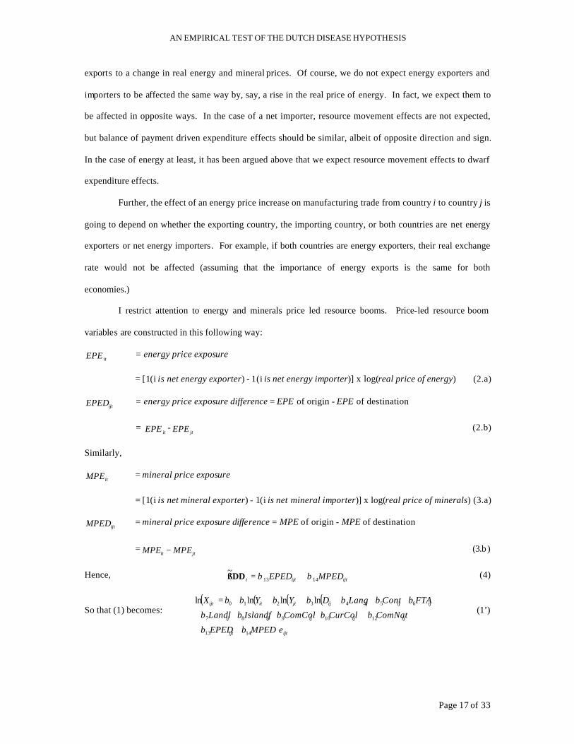
exports to a change in real energy and mineral prices. Of course, we do not expect energy exporters and

importers to be affected the same way by, say, a rise in the real price of energy. In fact, we expect them to

be affected in opposite ways. In the case of a net importer, resource movement effects are not expected,

but balance of payment driven expenditure effects should be similar, albeit of opposite direction and sign.

In the case of energy at least, it has been argued above that we expect resource movement effects to dwarf

expenditure effects.

Further, the effect of an energy price increase on manufacturing trade from country i to country j is

going to depend on whether the exporting country, the importing country, or both countries are net energy

exporters or net energy importers. For example, if both countries are energy exporters, their real exchange

rate would not be affected (assuming that the importance of energy exports is the same for both

economies.)

I restrict attention to energy and minerals price led resource booms. Price-led resource boom

variables are constructed in this following way:

itEPE = energy price exposure

= [1(i is net energy exporter) - 1(i is net energy importer)] x log(real price of energy) (2.a)

ijtEPED = energy price exposure difference = EPE of origin - EPE of destination

= itEPE -

jtEPE (2.b)

Similarly,

itMPE = mineral price exposure

= [1(i is net mineral exporter) - 1(i is net mineral importer)] x log(real price of minerals) (3.a)

ijtMPED = mineral price exposure difference = MPE of origin - MPE of destination

=jtit MPEMPE − (3.b )

Hence, ijtijtt MPEDEPED 1413

~ββ +=DDß (4)

So that (1) becomes: ( ) ( ) ( ) ( )

ijtijt

ijijijijij

ijijijijjtitijt

MPEDEPED

ComNatCurColComColIslandfLandl

FTAContLangDYYX

εββ

βββββ

βββββββ

+++

++++++

++++++=

1413

1210987

6543210 lnlnlnln (1’)


of 33

The real energy and mineral price index are denominated in 1995 dollars. I take these US dollar

world prices as exogenous to any single country. Very few exceptional countries such as Saudi Arabia for

oil and Chile for copper may cast some doubt on this assumption. It turns out no single observation is

exercising significant effect on the coefficient of interest according to DFBeta statitistics.

It could be argue that the real price of oil for example is not exogenous to a group of country like

OPEC. The basic problem with the cartel story was pointed out by a number of people, but perhaps most

forcefully by Cremer and Salehi-Isfahani (1989). Basically, OPEC did not to have the characteristics of an

effective cartel. It was too uneven from a cultural and political perspective. This cartel organization did

not even proceed to set output quotas until 1982, at a time when oil prices had already increased

substantially.

How can we explain for the 12-years of rising oil prices? In the late 70s, according to Paul

Krugman (2000), economists began to suggest a key element of the story was perverse supply responses.

Cremer and Salehi-Isfahani (1989) pointed out that oil differs from ordinary commodities in three

important ways: it’s exhaustible, its production is under government control, and it is a major source of

domestic revenue for the main oil exporters.

To reduce this potential endogeneity further, I use a world energy and mineral price index. In any

case, it should be noted that our concern should be endogeneity to manufacturing exports, i.e. our

dependent variable. It is unrealistically far fetched to assume material endogeneity of real world energy

prices to the manufacturing export performance of any specific country or cartel of countries. Historical

hindsight reveals that manufacturing export concerns have simply not been driving cartel price

coordination.

The second necessary identifying assumption is that being a country’s export “specialization” as

an energy or mineral exporter is independent of its manufacturing exports. At the margin, the level or share

of energy or mineral exports of a country is not exogenous to its manufacturing exports at all. What we are

identifying here is year on year price changes, and it could be assumed that a year-on-year drop in

manufacturing exports would drive a country into becoming a net exporter of energy, say. This is why I

will not make use of this information.


of 33

However, it is much safer to assume that the overall status of country as a net exporter or importer

of energy or mineral is rather exogenous to this country’s manufacturing exports, and reflects to a large

degree its geological endowment. As a further precaution against reverse causality, I only classifying as

net exporters (respectively importers) of, say, energy countries which never reverted to being a net importer

(respectively net exporter) over the period cover in my sample.

I followed the norm in the literature by first using ordinary least squares, albeit with standard

errors which are robust to clustering (since pairs of countries are likely to be highly dependent across

years). These results are available upon request but are not reported. They are not different in any

meaningful way from reported results. My preferred estimation strategy lays in panel data techniques. I

use both fixed and random effects estimators extensively below. I rely on the robust fixed effects “within”

estimator, which essentially adds a set of country-pair specific intercepts to the equation, and thus exploits

only the time series dimension of the data set around country-pair averages. I will also report all results

with and without extra time-dummies aimed at controlling for time trends in the explained and explanatory

variables.

3.3 The Data Set

The core of the data used in this paper comes from World Trade Data sets described in Feenstra, Lipsey

and Bowen (1997). The World Trade Database (WTDB) put together by Statistics Canada contains

bilateral trade flows for all countries over 1970-1992, recently updated up to 1997, classified according to

the Standard International Trade Classification. 98% of all trade is considered to be covered by this

database. Manufacturing exports are extracted by keeping exports falling under BEA 34-Industry Code 15-

29, and 31 to 34. The technical reason behind this choice of industrial categories is that I want to BEA

industry categories that are also classified as manufactured goods in the ISI classification. The economic

rational behind this choice is that I want a non-arbitrary rule to exclude industries that lay too closely to the

borderline between the primary and secondary sector.

The binary variables for common language, sharing a land border, belonging to the same regional

trade agreement, being colonies at time t, having ever been colonies after 1945 with the same colonizer,

remaining part of the same nation during the sample, the number of landlocked countries in the country-


of 33

pair, the number of island nations in the pair, and distance between counties are all taken from Glick and

Rose (2002). Real GDP and population data are taken from the World Bank (2002).

The series for the world price of energy and metals come from the International Financial

Statistics the I.M.F. (2002). These are nominal indexes with 1995 as base year. The real equivalent of

these series is used after deflating the nominal series by the US CPI (oil and most minerals are priced in

dollars). Shares of fuel and metals exports (respectively imports) in merchandise exports (respectively

imports) are taken from the World Bank (2002). A country is defined as a net exporter of fuel (respectively

metals) if its share of fuel exports (respectively metals) exceeds in all observed years its share of fuel

imports in merchandise imports (respectively metals). Similarly, a country is defined as a net importer of

fuel (respectively metals) if its share of fuel exports (respectively metals) exceeds in all observed years its

share of fuel imports in merchandise imports (respectively metals). While recognizing that merchandise

exports and imports are two different bases, no attempt is made at correcting this because the potential

impact of this wedge is judged to be immaterial, and that alternative data are incomplete.

Hence, practically energy and mineral price exposition indicators are computed as:

itEPE~ = [1(i net fuel exporter) - 1(i net fuel importer)] x log(real price of energy) (2.a)’

itEPM~ = [1(i net metals exporter) - 1(i net metals importer)] x log(real price of metals) (3.a)’

Finally, for purposes of sensitivity analysis, data on exchange rate regimes is taken from Ghosh,

A., A.-M. Gulde, J.D. Ostry, and H. Wolf9 (1996). They categorize regimes according to both the publicly

stated commitment of the central bank (their de jure classification) and the observed behavior of the

exchange rate (their de facto classification). Neither approach is fully adequate. A country that declares to

have a pegged exchange rate might in fact proceed to frequent changes in parity. Conversely, a country

might experience very small exchange rate movements, even though the central bank has no formal

requirement to uphold a parity.

The approach I take is to mix both criteria and not to classify as either floaters or fixers countries

that have a publicly stated commitment to some form currency rate fixing but there are infrequent parity

adjustments. If a country has any publicly stated commitment (be it a peg to a single, a SDR, an official or

9 I am thankful to Professor Holger Wolf from Center for German and European Studies, School of Foreign Service at Georgetown University for sharing his data.


of 33

a secret basket peg, or a cooperative arrangement like the EMS) and there is no change in parity, I classify

it as an effective fixer in that year. If a country has any publicly stated commitment but there are frequent

changes in parity, it is classified as an effective floater in that year. Lightly managed and independent

floats are classified as effective floaters, whereas heavily managed floats are classified as effective fixers in

that year.

4. Estimates

My preferred specification is that of country-pair fixed effects. Glick and Rose (2002) also recommend this

approach. I have also computed OLS results. They do not differ significantly and do not bring about

different conclusions from those derived here. However, fixed effects (and to a lesser extent random

effects) allows me to set aside concerns about omitted country (pair) characteristics. For example, time

invariant relative factor abundance characteristics of country pairs are implicitly controlled for the fixed

effect specification. Hence, there is no need to worry about, for example, the relative energy price

exposure variable simply picking up the effect of some country-pair specific omitted variable that would be

highly associated with one of the components of this variable.

Fixed effects allows me to make inferences about the effect of resource booms on changes in

manufacturing exports, rather than cross-country inferences regarding the effect of resource abundance on

manufacturing export specialization. The standards interpretation of fixed effects estimates is that they

measure the effect of a change in an explanatory variable, here the real energy price, on the steady-state of

a net fuel exporter. Finally, I use time-dummies to control for trends in the dependent and independent

variables. Whenever informative, I will report results with and without these time-dummies. It turns out

that the hypothesis of joint significance of time -dummies can always be rejected with very high confidence.

Their inclusion, however, does not alter results in any meaningful way. In the rest of this paper, I will

report both country-pair fixed and very often random effects. Random effect estimates allows checking the

coefficients for country pair characteristics. It is satisfying to check their consistency when changes in the

set-up are introduced.

Table 1 displays estimates of the gravity model using my dataset but excluding energy exposure

variables. The gravity model results are standard as well as intuitive. The model fits the data well,


of 33

explaining from half to two-thirds of the variation in manufacturing trade flows. The gravity coefficients

are economically and statistically significant with sensible interpretations. For instance, economically

larger and richer countries export more manufactured gooss; more distant countries do so less. A common

language, land border and membership in a regional trade agreement encourage manufacturing exports, as

does a common colonial history. Even the same nation coefficient is intuitively signed (contrary to Glick

and Rose 2002).

Note that the coefficient on own-GDP is greater than one as also greater than the coefficient on

partner-GDP as in Feenstra, Markusen and Rose’s (1998) simulations for differentiated goods. These

authors find that this is consistent rises as they move from homogenous to differentiated goods. This is

consistent with a more pronounced home market effect for differentiated goods; manufacturing can move

between more easily than production of resource-base homogenous goods (commodities.) Time dummies

cannot be rejected and so will be kept around.

In Table 2, I introduce resource price exposure variables. First, the introduction of the resource

price exposition variables does not affect the other coefficients. Linear fit is improved by 4-7 percent. The

energy price exposition difference turns out to be economically and statistically significant. The elasticity

of manufacturing exports to real energy price for a net fuel exporter is estimated to be .58-.65%. In other

words, a 1% increase in the real energy price will shave off around 2/3 of a percent of manufacturing

exports in net fuel exporters.

5. Sensitivity analysis

The rest of the empirical results reported in this paper aim at showing that extensive sensitivity analysis

does not materially undermine the reliability of the baseline results reported in Table 2. In particular, I

want to pay particular attention to the policy context in which resource booms / shocks take place. And

since, real exchange rate appreciation is thought to be the principal mechanism of operation of the Dutch

Disease, it makes sense to take a look at exchange rate regime as a way to see if how the results are affected

by policy.

Besides it often pointed out in the DD literature that regarding oil booms, one expects resource

movement effects to be shadowed by spending effects because of the “enclave economy” characteristics


of 33

and high capital intensity of oil exploitation activities. Hence we expect the role of the real exchange rate

to be important. Chen and Rogoff (2002) revisit the PPP puzzle in three OECD economies (Australia,

Canada, and New Zealand) where primary commodities represent a significant portion of their exports. For

Australia and New Zealand especially, they find that the price of their commodity exports — which they

also take to be generally exogenous to these small economies — has a strong and stable influence on their

real exchange rate, although this is not enough to explain for the PPP puzzle. Figure III shows evidence of

this using my dataset.

Therefore, in Table 3a, I segment the sample according to whether the origin, the destination or

both have effectively managed or unmanaged exchange rate regimes. It turns out that this type of data

segmentation affects this coefficient in a non-negligible way. However, this segmentation affects other

gravity model coefficients as well and this turns out to be true whether or not my resource price exposure

variables are present or not (unreported). I will leave the general issue of the effect of exchange rate

regimes on gravity estimates aside because it falls outside the scope of this paper. Instead, I will make here

tentative observations regarding the role of exchange rate regimes on the effect of energy price booms or

shocks. Obviously, these observations should be understood as a first rough cut at this question and with a

reasonable amount of skepticism.

Diagram I helps picture the taxonomy that I employ here and its effect on the coefficient on

resource price exposure. Let’s leave the issue of statistical significance aside at first. In general, currency

management by a country seems to mitigate DD effects keeping the trading partner’s exchange rate policy

constant. A country seems to be less subject to DD effects vis -à-vis a trade partner that floats. If the

trading partner is heavily managing its currency, then the origin country will be less subject to DD effects if

it manages its currency as well. Looking at things from the point of view of statistical significance, one is

lead to conclude that DD effects don’t seem to be a concern vis -à-vis countries that do not manage their

currencies. Also, this also the case if both trading partners manage their currencies. The worst case

scenario is that of a floater trading with a currency manager. And the best scenarios are when trading

partners have similar exchange rate policies.

To check the sensibility of these observations to the method of estimation and to whether or not I

include time -dummies in the set of explanatory variables, Table 3b shows a doubly entry taxonomy of


of 33

method of estimation vs. exchange rate regimes and gives the corresponding estimate for the coefficient on

the energy price exposure variable. It turns out that the fixed effect with time-dummies is a bit of an acid

test when combined with sample segmentation according to exchange rate regime. This is of course the

consequence of opting for the most demanding specification as baseline results.

The flip side of this is that, naturally, other, less demanding, specifications use less degrees of

freedom and allow estimating my coefficient of interest with more precision. The outcome is that when

one relaxes the estimation method a little, the DD reappears more strongly in many cases where it looked

like insignificant in the baseline results. Interestingly, if one were to rank the different coefficient estimates

across exchange rate regimes for each different methods of estimation, our previous observations regarding

the relative desirability of different exchange rate regime combinations are in general unchanged.

Finally, Table 3c, I take the reverse approach consisting in excluding observations belonging to

the same combinations of exchange rate regimes. DFBetas indicate the extent to which the observed

change in the coefficient on energy price exposure are statistically significant. This is the standard way to

look for outliers, either individually or as a group.

If these results are confirmed by future research, they are indicative of the possibility for currency

managers to “export” their DD. Recall that the effects of energy shock to a net energy importer has so far

been modeled as the mirror effect of the effect of the same boom on a net energy exporter. This naturally

begs for testing whether these effects indeed work in opposing direction. A DFBeta value above 2 is

considered suspicion of an outlier or a group of outliers. Table 3c tabulates DFBetas across specifications

and excluded combinations of exchange rate regime. Diagram II helps visualize the corresponding

taxonomy of cases.

All DFBetas are negative indication that in all case the price exposure coefficient is strengthened

(in absolute terms) by the exclusion of the proposed combinations of exchange rate regimes. In most cases,

however, the effect on the energy coefficient is insignificant. The only combination that is systematically

significant is the case where the origin fixes, again indicating that exchange rate management helps soothe

DD effects. I will keep this observation as the main conclusion of this exercise in sensitivity analysis.

Other combinations of exchange rates either have no significant effect on the coefficient of interest or only

in some of the specifications. It is important to emphasize again that exclusion of any of the combinations


of 33

investigated would strengthen the magnitude on the energy price exposure variable. That is why, since the

null hypothesis is the insignificance of this coefficient, none of these combinations is hereafter excluded

from the sample.

In Table 4, I turn to another issue. Let’s take again a look at (4) which defined our resource price

exposure term, DDß~ and let’s expand the term ijtEPED . There are three ways to do so.

The first one is a straight application of (2.b).

ijtEPED = itEPE -

jtEPE . (5)

Let’s expand these terms further by making use of (2.A)

ijtEPED = [1(I net energy exporter) - 1(I net energy importer)] x log(real price of energy) – [1(J net energy

exporter) - 1(J net energy importer)] x log(real price of energy)

= [1(I net energy exporter) - 1(J net energy exporter)] x log(real price of energy) + (-1)[1(I net

energy importer) - 1(J net energy importer)] x log(real price of energy)

= MtEPE (-1) +X

tEPE (6)

Finally, I can of course fully decompose the term ijtEPED into its four original compotents, i.e.:

ijtEPED = itEPE -

jtEPE = Mjt

Mjt EPE (-1) EPE (-1) +++ X

itX

it EPEEPEi (7)

In essence the energy price exposure difference variable can be expanded according to whether the energy

price boom affects the exporting country or the importing country as in (5), or according to whether the

energy price boom is to a net exporter or a net importer of energy (6), or according to both criteria as in (7).

Diagram III helps visualize the taxonomy proposed in Table 4 as the effect of decomposing real energy

price exposure.

Disaggregating our exposure variable yields intuitive results. Energy price booms at the origin

hurt its manufacturing exports while booms in the destination country (by inducing a real depreciation)

actually boost manufacturing exports (in the origin country.) Perhaps surprisingly, energy boom at the

destination are estimated to have a large impact than booms in the orig in country (in absolute value.)

Booms affect net energy exporters’ manufacturing exports a lot more than shocks help. net energy

importers (even keeping GDP constant). Allowing these weaker reverse effects on energy importers to be

lumped into the baseline energy price exposure difference variable, reassuringly works against my


of 33

conclusions. In other words, it is not the case that some hypothetical reverse Dutch disease effect is driving

the side of the baseline coefficient, all the opposite . The effect on the component related to net exporters is

in fact very strong, with a 1.63 energy price elasticity of manufacturing exports (in absolute value, of

couse.)

Complete disagregation, intuitively combines the sign of results obtained from both types of

partial disaggregating. Hence, logically the strongest, here positive, effect is obtained for an energy price

boom when the destination is a net exporter. The smallest effect is obtained for a shock to an energy

importing destination country. This is not consistent with the observation that shocks to the destination are

larger than to the origin. However, a statistical hypothesis of this hypothesis can only reject the null

hypothesis with a 10% significance level. Since we should not reject this hypothesis, we can satisfy

ourselves with the intuitive character of the small effect for a shock to an energy importing destination

country.

Tests show that one can reject the null hypothesis of no statistical significance for disaggregating

effects on exporters from those on importers. In general, tests are all highly indicative of the statistical

significance of the unrestricted model (4.3). This is perhaps pleading for disaggregating coefficient in the

so-called baseline results, and then focusing on the coefficient on domestic booms in a net exporter. If I

opted for this approach, I would actually strengthen my conclusions, and report a higher estimate of 1.63

for the energy price elasticity of manufacturing exports. Instead, I will report the aggregated coefficient for

the sake of simplicity and consider it as a lower bound on the effect on would effect from on an energy

boom in a net exporter.

Table 5 tabulates key results when instead of working is real US dollars, all economic variables

are evaluated instead in the origin country’s currency or the destination country’s currency. Baseline

results in US dollars are reproduced for comparison purposes. The transformation of the dollar figure is

done using the real exchange rate index with 1995=100 as base year. So, foreign currency variables are

evaluated in 1995 US dollar equivalent. In any case, country pair dummies would absorb the effect of

differing currency units, so there is no concern about pooling observations in difference currency units.

Measuring economic variables in the origin’s currency improves the linear fit and lowers the

estimated real energy price elasticity. This coefficient remains highly significant, however. Measuring


of 33

economic variables in the destination’s currency further improves the linear fit but strengthens estimated

real energy price elasticity beyond that of baseline dollar estimates.

The coefficient changes are intuitive. Given the real appreciation of the domestic currency likely

to follow a boom in a net energy exporter, destination’s imports are likely to decrease all the more when

expressed in destination’s depreciated currency. Conversely, origin’s exports are likely to deteriorate less

all the more when expressed in origin’s appreciated currency. Indeed, in all three cases the real exchange

rate appreciation takes place; it is only the unit of measurement we are changing.

Generally, changing currency units for economic variables does not affect key results. The US

dollar baseline results emphasized in this paper turn out to be an intermediary case. It is kept as baseline

case because it is the standard approach in the gravity literature, and there are obvious benefits to working

in a third country’s currency as it avoids some of the interpretation problems associated with potentially

volatile exchange rates.

6. Conclusion (preliminary – too close to the end of the introduction)

In the light of the endogeneity of commodity exports to manufacturing trade, world real energy and mineral

prices are used to identify price led resource booms. Indeed, world commodity prices can be safely

assumed to be exogenous to any single country’s manufacturing exports. With this identifying assumption

in hand, the real energy price elasticity of manufacturing exports in net energy exporters is estimated to be

around .6%. In other words, a one percent increase in the price of energy will, everything else held

constant, decrease a net energy exporter’s real manufacturing exports by 0.6%. This elasticity estimate is

exceptionally significant and the corresponding confidence interval very small.

Neither segmenting the data based on effective exchange rate regime nor decomposing the

variable of interests nor changing currency units of measurement overturns results. However, it is learned

from sensitivity analysis that exchange rate management might allow countries to partially offset some of

the Dutch Dis ease effects resulting from an energy price led boom. It other words, exchange rate

management may allow net energy exporters to export some of the Dutch Disease effects, as is thought to

have worked successfully in Indonesia (Roemer, 1994). Also, DD effects are strongest with net energy

exporters rather than net importers. Booms occurring in the destination country seem to have comparable


of 33

effects (but of opposite sign, obviously) on manufacturing exports by the origin, than booms taking place in

the origin country.

The main result found is this paper is in some way surprising in the state of the DD literature. I

find strong evidence of the DD in the world trade data. Price-led resource booms, and particularly energy

booms, have systematically tended to hurt energy exporters’ manufacturing exports. So, in contrast with

the existing literature, this paper casts away doubts about the empirical relevance of the DD, particularly

regarding energy producers. It is intuitive, however, that by juxtaposing the marginally convincing

evidence found in numerous countries, one be able to either reject or accept the DD hypothesis10.

One should be careful in not over-interpreting these results reported in this paper, however. In

most cases, booms result in increased GDP levels, and hence welfare, for energy producers. That’s not the

question at stake in this paper. Further, one only needs to worry about the DD insofar as there is indeed

something desirable about having a large proportion of manufacturing exports. There is, however,

evidence that productivity growth can sometimes be very strong in resource extraction industries, at least in

industrialized countries. And the role of that manufacturing may play over the primary sector may vary

from country to country, because of the possibility of factor intensity reversal, for example.

On the other hand, there is a widespread assumption in the structural tradition of the development

literature that industrialization should be per se an economic development goal. More recently, Matsuyama

(1992), Sachs and Warner (1995, 1999), and their followers, have explicitly modeled economic growth as a

function of the relative size of the manufacturing sector. It is not the purpose of this paper to settle this

issue. Rather, the statistic and economic significance of the result found here lead me to argue in favor of

careful future empirical testing of the effect of sectoral changes in output and exports, and more specifically

those resulting from resource booms, on aggregate productivity and economic growth.

Now that the effect of resource booms on energy exporters’ manufacturing exports is established,

there is urging need, in the author’s view, to test whether, if, how and why this de-industrialization would

result in slower technological progress. As far as industrial, public finance, energy and development policy

formulation is concerned, the results are unambiguous: resource boom are very likely to result in de-

10 If authors in the DD empirical literature systematically reported comparable estimates of the effect of resource shocks on manufacturing exports, it would be interesting to see if the same conclusion is reached through meta-analysis. Such is far from the case, unfortunately


of 33

industrialization, and if this is an economic or political concern, or both, then energy net exporters (and to

a less extent energy net importers, actually) should take account of this balance of payment constraint.

7. References

ANDERSON, J. (1979) “A Theoretical Foundation for the Gravity Equation,” American Economic Review,

69(1), March, 106-116.

ASCHER, W., Why Governments Waste Natural Resources: Policy Failures in Developing Countries, The

John Hopkins University Press: Baltimore and London, 1999.

BARKER T. AND V. BRAILOVSKY, Oil or Industry? Energy, Industriliasation and Economic Policy in

Canada, Mexico, the Netherlands, Norway and the United Kingdom, London: Academic Press,

1981

BARKER T., “Chapter 12: Policy Issues in Energy-rich Economies” IN BARKER T. AND V. BRAILOVSKY, Oil

or Industry?, 1981

BERGSTRAND, J.H. (1985) “The Gravity Equation in International Trade: some Microeconomic Foundations

and Empirical Evidence,” Review of Economics and Statistics, 67, August, 474-481.

BERGSTRAND, J.H. (1989) “The Generalised Gravity Equation Monopolistic Competition, and the Factor-

Proportions Theory in International Trade,” Review of Economics and Statistics, 71, February,

143-153.

BUITER, W. AND M. MILLER, “The Thatcher Experiment: The First Two Years”, Brookings Papers on

Economic Activity, Vol. 1981, No. 2. (1981), pp. 315-367

BUITER, W. AND M. MILLER, “Changing the Rules: Economic Consequences of the Thatcher Regime”,

Brookings Papers on Economic Activity, Vol. 1983, No. 2. (1983), pp. 305-365.

CAIRNES, J.E., “The Australian Episode”, Frazer’s Magazine (1859), reprinted in Taussig, F. W. (ed),

Selected Readings in International Trade and Tariff Problems, New York: Ginn and Company,

1921

CHEN, Y.-C. AND K. ROGOFF, “Commodity Currencies and Empirical Exchange Rate Puzzles”,

International Monetary Fund Working Paper 02/27, February 2002.

CORDEN, W.M., “James Meade 1907-1995.” Economic Record 72.217, June 1996: 172-4.


of 33

CORDEN W.M. “Booming Sector and Dutch Disease Economics: Survey and Consolidation” Oxford

Economic Papers, vol. 36, p. 359-380 (1984). Reprinted in W.M. Corden, International Trade

Theory and Policy. Edward Elgar Publishing, 1992.

CREMER AND SALEHI-ISFAHANI, "The Rise and Fall of Oil Prices: A Competitive View", Annales

d'Economie et de Statistiques, no 15/16, July-December 1989, 427-454

DANIELPH. , “Editorial”, IDS Bulletin (October 1986), Mineral Exporters in Boom and Slump , pp. 1-9.

DORRANCE, GR., AND R. LEESON, “Obituary: James Edward Meade CB FBA, 1907-1995,” Economics

Department Murdoch University Working Paper No. 161, July 1997,

http://cleo.murdoch.edu.au/teach/econs/wps/161.html

ELLMAN, M. (1981), “Natural Gas, Restructuring and Re-industrialization: The Dutch Experience of

Industrial Policy” in BARKER T. AND V. BRAILOVSKY, Oil or Industry?, 1981

ENGEL, CH. AND J. ROGERS (1996) “How Wide is the Border?” American Economic Review 86-5, 1112-

1125.

FEENSTRA, R., R.E. LIPSEY, AND H.P. BOWEN, “World Trade Flows, 1970-1992, with Production and Tariff

Data,” NBER Working Paper No.w5910, Issued in January 1997.

FORSYTH, P. (1985), “Booming Sectors and Structural Change in Australia and Britain: A Comparison”, in

PETER NEARY AND SWEDER VAN WIJNBERGEN (Eds.), Natural Resources and the Macroeconomy .

FORSYTH P.J., ST . J. NICHOLAS, “The Decline of Spanish Industry and the Price revolution: A Neoclassical

Analysis ”, Journal of European Economic History, 12 (winter), 601-9.

FRANKEL, J. AND D. ROMER (1999) “Does Trade Cause Growth?” American Economic Review 89-3, 379-

399.

FRANKEL, J. AND SH.-J. WEI (1993) “Trade blocs and currency blocks” NBER Working Paper No. 4335,

published in The Monetary Future of Europe (Guillermo de la Dehaza et al eds.; London: CEPR).

GAUZIER, A., “Prices and output in two oil based economies: the Dutch disease in Iran and Nigeria”, IDS

Bulletin (October 1986), pp. 14-21.

GELB, A., Oil Windfalls: Blessing or Curse?, Oxford University Press, New York., 1988.

GLICK R., A AND ROSE, A. K., “Does a currency union affect trade? The time-series evidence”, European

Economic Review, Volume 46, Issue 6, June 2002, Pages 1125-1151


of 33

GHOSH, A., A.-M. GULDE, J.D. OSTRY, AND H. WOLF (1996), Does the Exchange Rate Regime Matter for

Inflation and Growth?, International Monetary Fund: Washington D.C.

HELPMAN, E., “The Factor Content of Foreign Trade.” Economic Journal, March 1984, 94(373), pp. 84–94.

INTERNATIONAL MONETARY FUND, International Financial Statistics(IFS), 2002.

JAZAYERI, A., “Prices and output in two oil based economies: the Dutch disease in Iran and Nigeria”, IDS

Bulletin (October 1986), pp. 14¯21.

KRUGMAN, P. (1987) “The Narrow Moving Band, the Dutch Disease and The Competitive Consequences

of Mrs. Thatcher on Trade in the Presence of Dynamic Scale Economies” in The Journal of

Development Economics. vol. 27, p. 41-55.

KRUGMAN, P., The energy price revisited, http://web.mit.edu/krugman/www/opec.html, March, 2000.

KAMAS, L. “Dutch disease economics and the Colombian export boom”, World Development, Volume 14,

Issue 9, September 1986, Pages 1177-1198.

KARLYGASH KURALBAYEVA, ALI M. KUTAN, AND MICHAEL L. WYZAN, “Is Kazakhstan vulnerable to the

Dutch Disease?”, Zentrumfür Europäische Integrationsforschung Working Paper B29 2001.

KREMERS, J., “Booming Sectors and Structural Change in Australia and Britain: A Comparison”, in PETER

NEARY AND SWEDER VAN WIJNBERGEN (Eds.), Natural Resources and the Macroeconomy , 1985.

LEAMER, E. AND J. LEVINSOHN (1995) “International Trade Theory: The Evidence” in The Handbook of

International Economics, vol. III (edited by GROSSMAN, G., AND K. ROGOFF).

LOONEY, R. E., “Oil revenues and viable development: impact of the Dutch disease on Saudi Arabian

diversification efforts” American Arab Affairs (Winter 1988/99), pp. 25-35.

LOONEY, R. E. “Diversification in a small oil exporting economy; the impact of the Dutch disease on

Kuwait's industrialization”, Resources Policy, Volume 17, Issue 1, March 1991, Pages 31-41

MCMAHON G., “The Natural Resource Curse: Myth or Reality?” Economic Development Institute, the

World Bank, Washington, D.C., Final Draft, October 21, 1997.

MACGARVIE, M., “Do Firms Learn from International Trade? Evidence from French Micro-Data”,

manuscript presented at the Macroeconomics Seminar, Un iversity of California at Berkeley,

August 29, 2002..


of 33

MADDOCK, R. AND I. MCLEAN (1983), “Supply Side Shocks. The Case of Australian Gold”, The Journal of

Economic History, Vol. 44, No. 4. (Dec., 1984), pp. 1047-1067

MATSUYAMA, K., “Agricultural Productivity, Comparative Advantage, and Economic Growth,” Journal of

Economic Theory, 58 (1992), 317-334.

MEADE, J. AND E. RUSSEL, “Wage Rates, the Cost of Living, and the Balance of Payments,” Economic

Record , 33, 1957: 23-28, reprinted in MEADE, J., The collected papers of James Meade, Volume 3,

Edited by S. HOWSON, Winchester, Mass., London and Sydney, Unwin Hyman, 1988

PÖYHÖNEN, PENTTI (1963) “A Tentative Model for the Volume of Trade between Countries”

Weltwertschaftliches Archiv 90 (1), 93-99.

ROCA A. M., “Dutch Disease and Banana Exports in the Colombian Caribbean, 1910 – 1950”, paper

presented at the meeting of the Latin American Cliometric Society (LACLIO) in Cartagena,

Colombia, August 27-28, 1999.

ROEMER M., “Dutch disease in developing countries: swallowing bitter medicine”. In: MATS LUNDAHL,

Editor, The Primary Sector in Economic Development: Proceedings of the Seventh Arne Ryde

Symposium29-30 August 1983, Croom Helm, London (1985).

ROEMER M., “Dutch Disease and Economic Growth: The Legacy of Indonesia”, Development Discussion

Paper No. 489, Harvard Institute for International Development, June 1994: pp. 1-14.

ROSE, A. K., “One money, one market: the effect of common currencies on trade”, Economic Policy,

Volume 15: Issue 30, 2000, pp. 7-46.

ROSE, ANDREW K. (2001) “Currency Unions and Trade: The Effect is Large”, Economic Policy.

ROSS, A. CL., “The United Kingdom’s Experience with North Sea Oil and Gas”, IDS Bulletin (October

1986), pp. 14-21.

ROSE, ANDREW K. AND ERIC VAN WINCOOP (2001) “National Money as a Barrier to Trade: The Real Case

for Monetary Union”, American Economic Review.

SABAH, M. AL- “The ‘Dutch disease’ in an oil exporting country: Kuwait.” OPEC Review (Summer 1988).

SACHS, F. AND W. BRANSON, “Changing the Rules: Economic Consequences of the Thatcher Regime.

Comments and Discussion”, Brookings Papers on Economic Activity, Vol. 1983, No. 2. (1983),

pp. 366-379.


of 33

SACHS, J., A. WARNER, AND M. ANDREW “Natural Resource Intensity and Economic Growth,” in

Development Policies in Natural Resource Economies, JÖRG MAYER, BRIAN CHAMBERS, AND

AYISHA FAROOQ EDS., Edward Elgar, Cheltenham, UK and Northampton, Massachusetts , 1999.

First published as “Natural Resource Abundance and Economic Growth,” NBER Working Paper

Series, 5398, (1995), 1-47.

SPATAFORA N. AND A. WARNER, “Macroeconomic and Sectoral Effects of Terms -of-Trade Shocks - The

Experience of the Oil-Exporting Developing Countries”, IMF Staff Paper 134/99, October 1999.

Current version November 2001, presented on August 22 2002 at the European Economic

Association meeting.

SPILIMBERGO, A. (1999), “Copper and the Chilean Economy: 1960-98,” IMF Working Paper No. 99/57,

International Monetary Fund, April 1999: pp. 1-33.

TINBERGEN, J. (1962) Shaping the World Economy: Suggestions for an International Economic Policy

(New York).

VAN WIJNBERGEN, SW., “The Dutch Disease: A Disease After All?” Economic Journal 94, 41-55, 1984a.

VAN WIJNBERGEN, SW., “Inflation, Employment, and the Dutch Disease in Oil-Exporting Countries: A

Short-Run Disequilibrium Analysis ”, The Quarterly Journal of Economics, Vol. 99, No. 2. (May,

1984b), pp. 233-250.

WARR, P. G., “Indonesia’s other Dutch Disease”, in PETER NEARY AND SWEDER VAN WIJNBERGEN (Eds.),

Natural Resources and the Macroeconomy , 1985.

WORLD BANK, World Development Indicators, World Bank, Washington D.C., 2002.

Table 1: Gravity model regressions Dependent Variable: Real manufacturing trade between

country of origin and country of destination Method of estimation Random

Effects Fixed

Effects Random Effects

Fixed Effects

(1.1) (1.2) (1.3) (1.4)

1.31 1.91 1.34 1.44 Log real GDP of origin (0.01)*** (0.02)*** (0.01)*** (0.02)***

0.80 1.40 0.83 0.99 Log real GDP of destination (0.01)*** (0.02)*** (0.01)*** (0.02)***

-1.23 -1.25 Log of distance (0.03)*** (0.03)***

0.63 0.65 1 (Common Language) (0.06)*** (0.06)***

0.37 0.35 1 (Common Border) (0.13)*** (0.13)***

0.83 0.73 1 (Regional Trade Agreement) (0.11)*** (0.11)***

1.06 1.15 1 (Common colonizer) (0.07)*** (0.07)***

1.46 1.41 1 (Colonial relationship) (0.16)*** (0.16)***

2.26 2.34 1 (Same nation in the sample) (0.43)*** (0.43)***

-0.15 -0.13 # of land-locked countries in pair (0.04)*** (0.04)***

Constant -39.32 -77.74 -40.44 -56.62 (0.36)*** (0.81)*** (0.32)*** (0.34)***

Time dummies p(F)=.00 p(F)=.00 Excluded Excluded Observations 136,073 137,755 136,073 137,755

Country pairs 9,736 102,32 9,736 10,232

R-squared 0.64 0.51 0.64 0.52

Standard errors in parentheses * significant at 10%; ** significant at 5%; *** significant at 1%

Estimated coefficients and standard errors are not reported for time dummies, instead a the p-value of a joint significance test is reported.

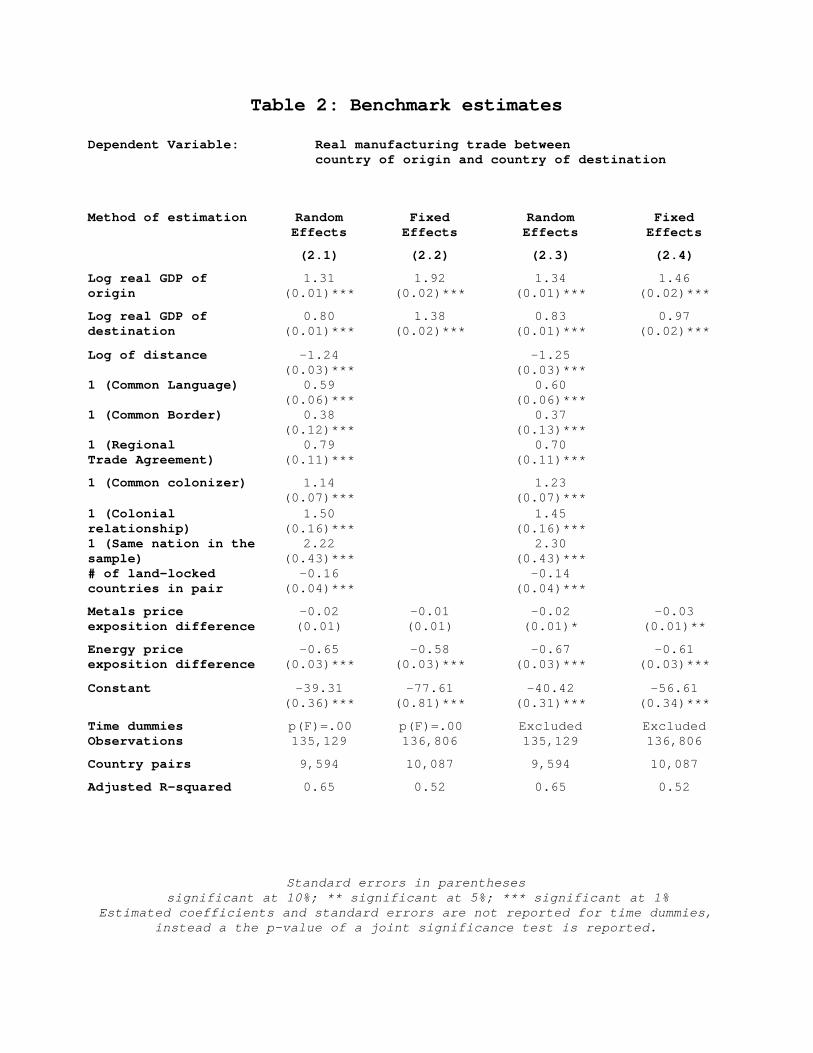
Table 2: Benchmark estimates Dependent Variable: Real manufacturing trade between

country of origin and country of destination Method of estimation Random

Effects Fixed

Effects Random Effects

Fixed Effects

(2.1) (2.2) (2.3) (2.4)

1.31 1.92 1.34 1.46 Log real GDP of origin (0.01)*** (0.02)*** (0.01)*** (0.02)***

0.80 1.38 0.83 0.97 Log real GDP of destination (0.01)*** (0.02)*** (0.01)*** (0.02)***

-1.24 -1.25 Log of distance (0.03)*** (0.03)***

0.59 0.60 1 (Common Language) (0.06)*** (0.06)***

0.38 0.37 1 (Common Border) (0.12)*** (0.13)***

0.79 0.70 1 (Regional Trade Agreement) (0.11)*** (0.11)***

1.14 1.23 1 (Common colonizer) (0.07)*** (0.07)***

1.50 1.45 1 (Colonial relationship) (0.16)*** (0.16)***

2.22 2.30 1 (Same nation in the sample) (0.43)*** (0.43)***

-0.16 -0.14 # of land-locked countries in pair (0.04)*** (0.04)***

-0.02 -0.01 -0.02 -0.03 Metals price exposition difference (0.01) (0.01) (0.01)* (0.01)**

-0.65 -0.58 -0.67 -0.61 Energy price exposition difference (0.03)*** (0.03)*** (0.03)*** (0.03)***

Constant -39.31 -77.61 -40.42 -56.61 (0.36)*** (0.81)*** (0.31)*** (0.34)***

Time dummies p(F)=.00 p(F)=.00 Excluded Excluded Observations 135,129 136,806 135,129 136,806

Country pairs 9,594 10,087 9,594 10,087

Adjusted R-squared 0.65 0.52 0.65 0.52

Standard errors in parentheses significant at 10%; ** significant at 5%; *** significant at 1%


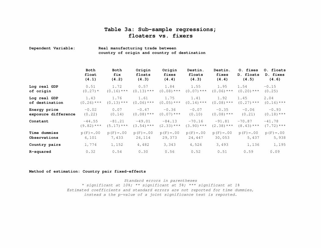
Table 3a: Sub-sample regressions; floaters vs. fixers

Dependent Variable: Real manufacturing trade between

country of origin and country of destination Both

float Both fix

Origin floats

Origin fixes

Destin. floats

Destin. fixes

O. fixes D. floats

O. floats D. fixes

(4.1) (4.2) (4.3) (4.4) (4.3) (4.4) (4.5) (4.6)

0.51 1.72 0.57 1.84 1.55 1.95 1.54 -0.15 Log real GDP of origin (0.27)* (0.16)*** (0.13)*** (0.08)*** (0.07)*** (0.06)*** (0.20)*** (0.25)

1.43 1.76 1.61 1.75 1.41 1.92 1.45 2.04 Log real GDP of destination (0.26)*** (0.13)*** (0.06)*** (0.05)*** (0.14)*** (0.08)*** (0.27)*** (0.16)***

-0.02 0.07 -0.47 -0.36 -0.07 -0.35 -0.06 -0.93 Energy price exposure difference (0.22) (0.14) (0.08)*** (0.07)*** (0.10) (0.08)*** (0.21) (0.18)***

Constant -44.55 -81.21 -49.01 -84.13 -70.16 -91.81 -70.87 -41.78 (9.82)*** (5.17)*** (3.54)*** (2.33)*** (3.90)*** (2.38)*** (8.43)*** (7.72)***

Time dummies p(F)=.00 p(F)=.00 p(F)=.00 p(F)=.00 p(F)=.00 p(F)=.00 p(F)=.00 p(F)=.00 Observations 6,101 7,433 26,114 29,373 24,447 30,053 5,437 5,938

Country pairs 1,774 1,152 4,482 3,343 4,526 3,493 1,136 1,195

R-squared 0.32 0.54 0.30 0.56 0.52 0.51 0.59 0.09

Method of estimation: Country pair fixed-effects

Standard errors in parentheses * significant at 10%; ** significant at 5%; *** significant at 1%


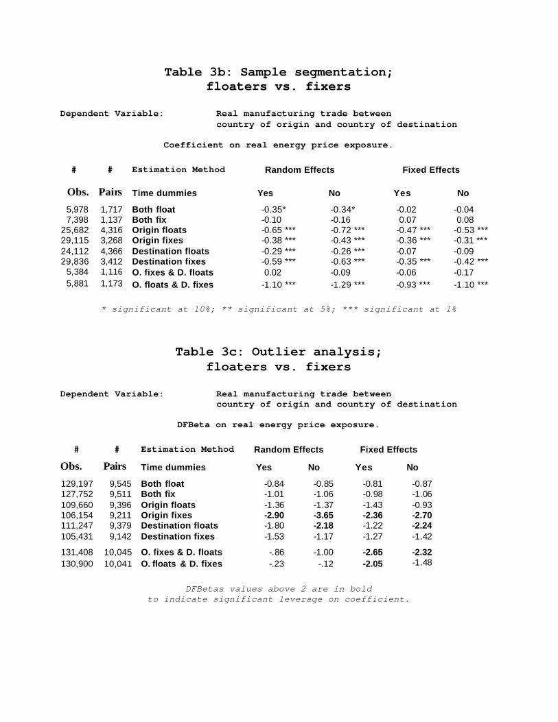
Table 3b: Sample segmentation; floaters vs. fixers


country of origin and country of destination

Coefficient on real energy price exposure.

# # Estimation Method Random Effects Fixed Effects

Obs. Pairs Time dummies Yes No Yes No

5,978 1,717 Both float -0.35* -0.34* -0.02 -0.04 7,398 1,137 Both fix -0.10 -0.16 0.07 0.08

25,682 4,316 Origin floats -0.65 *** -0.72 *** -0.47 *** -0.53 *** 29,115 3,268 Origin fixes -0.38 *** -0.43 *** -0.36 *** -0.31 *** 24,112 4,366 Destination floats -0.29 *** -0.26 *** -0.07 -0.09 29,836 3,412 Destination fixes -0.59 *** -0.63 *** -0.35 *** -0.42 ***

5,384 1,116 O. fixes & D. floats 0.02 -0.09 -0.06 -0.17 5,881 1,173 O. floats & D. fixes -1.10 *** -1.29 *** -0.93 *** -1.10 ***

* significant at 10%; ** significant at 5%; *** significant at 1%

Table 3c: Outlier analysis; floaters vs. fixers



DFBeta on real energy price exposure.

# # Estimation Method Random Effects Fixed Effects

Obs. Pairs Time dummies Yes No Yes No

129,197 9,545 Both float -0.84 -0.85 -0.81 -0.87 127,752 9,511 Both fix -1.01 -1.06 -0.98 -1.06 109,660 9,396 Origin floats -1.36 -1.37 -1.43 -0.93 106,154 9,211 Origin fixes -2.90 -3.65 -2.36 -2.70 111,247 9,379 Destination floats -1.80 -2.18 -1.22 -2.24 105,431 9,142 Destination fixes -1.53 -1.17 -1.27 -1.42

131,408 10,045 O. fixes & D. floats -.86 -1.00 -2.65 -2.32 130,900 10,041 O. floats & D. fixes -.23 -.12 -2.05 -1.48

DFBetas values above 2 are in bold

to indicate significant leverage on coefficient.

Table 4: Asymmetric effects of booms vs. crunches; Separate effects for origin vs. destination

Dependent Variable: Real manufacturing trade between country of origin

and country of destination Method of estimation Fixed

Effects Fixed

Effects Fixed

Effects

(4.1) (4.2) (4.3)

1.92 1.91 1.92 Log real GDP of origin (0.02)*** (0.02)*** (0.02)***

1.38 1.38 1.38 Log real GDP of destination (0.02)*** (0.02)*** (0.02)***

-0.52 Energy price shock (origin) (0.05)***

0.62 Energy price shock (destination) (0.04)***

-1.63 Energy price shock to energy exporter (0.08)***

.17 Energy price shock to energy importer (.04)

-1.29 Energy price shock to energy exporter (origin) (0.13)***

0.27 Energy price shock to energy importer (origin) (0.06)***

1.90 Energy price shock to energy exporter (destination) (0.11)***

-0.08 Energy price shock to energy importer (destination) (0.06) Time dummies p(F)=.00 p(F)=.00 p(F)=.00 Observations 137,755 137,755 137,755

Country pairs 102,32 102,32 10,232

R-squared 0.52 0.52 0.52

H0: destination = - origin 0.11 N/A 0.00

H0: exporter = - importer N/A 0.00 0.00

Joint Hypothesis N/A N/A 0.00

LR Test (H1 = (8.3)) 0.00 0.00 N/A

Standard errors in parentheses

* significant at 10%; ** significant at 5%; *** significant at 1% Estimated coefficients and standard errors are not reported for time dummies,

instead a the p-value of a joint significance test is reported.

Table 5: Reduced form gravity model regressions Sensitivity analysis: currency definition



Estimation Method

Currency Definition

Metal price

Standard errors

Energy price

Standard errors

# Obs.

# Pairs R²

(9.1) RE + T Dummies Dollars -0.02 (0.01) -0.65 (0.03)*** 135,129 9,594 0.65 (9.2) RE + T Dummies Origin’s currency. -0.01 (0.01) -0.59 (0.03)*** 132,322 9,474 0.68 (9.3) RE + T Dummies Destination’s currency -0.03 (0.01)** -0.72 (0.03)*** 132,462 9,474 0.71

(9.4) FE + T Dummies Dollars -0.01 (0.01) -0.58 (0.03)*** 136,806 10,087 0.52 (9.5) FE + T Dummies Origin’s currency. 0.01 (0.01) -0.46 (0.03)*** 133,975 9,964 0.61 (9.6) FE + T Dummies Destination’s currency -0.04 (0.01)*** -0.68 (0.03)*** 134,034 9,964 0.63

(9.7) RE Dollars -0.02 (0.01)* -0.67 (0.03)*** 135,129 9,594 0.65 (9.8) RE Origin’s currency. 0.01 (0.01) -0.57 (0.03)*** 132,322 9,474 0.68 (9.9) RE Destination’s currency -0.03 (0.01)* -0.77 (0.03)*** 132,462 9,474 0.71

(9.10) FE Dollars -0.03 (0.01)** -0.61 (0.03)*** 136,806 10,087 0.52 (9.11) FE Origin’s currency. 0.02 (0.01) -0.42 (0.03)*** 133,975 9,964 0.61 (9.12) FE Destination’s currency -0.06 (0.01)*** -0.81 (0.03)*** 134,034 9,964 0.64

* significant at 10%; ** significant at 5%; *** significant at 1% Notes: All currencies deflated by their own consumer price deflators. Real trade and GDP though unreported have also been converted to the same currency.

Figure I : Manufacturing trade as a share of GDP

0%

2%

4%

6%

8%

10%

12%

14%

16%

18%

19701971

19721973

19741975

19761977

19781979

19801981

19821983

19841985

19861987

19881989

19901991

19921993

19941995

Year

Rea

l Man

ufac

turi

ng E

xpor

ts :

Rea

l GD

P

90

100

110

120

130

140

150

Rea

l Oil

Pri

ce in

$U

S (

P19

95=1

00)

The Netherlands United Kingdom

France Germany

Real price of energy (1995 base)

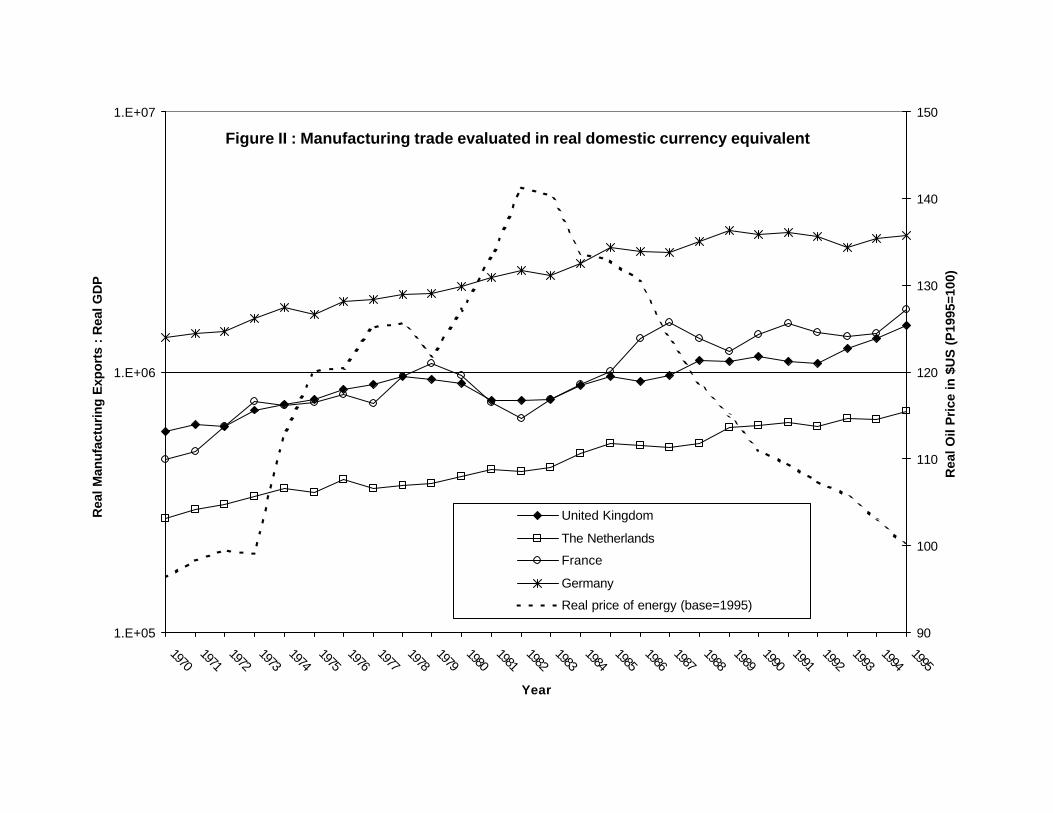
Figure II : Manufacturing trade evaluated in real domestic currency equivalent

1.E+05

1.E+06

1.E+07

19701971

19721973

19741975

19761977

19781979

19801981

19821983

19841985

19861987

19881989

19901991

19921993

19941995

Year

Rea

l Man

ufac

turi

ng E

xpor

ts :

Rea

l GD

P

90

100

110

120

130

140

150

Rea

l Oil

Pri

ce in

$U

S (

P19

95=1

00)

United Kingdom

The Netherlands

France

Germany

Real price of energy (base=1995)

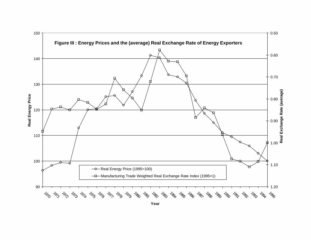
Figure III : Energy Prices and the (average) Real Exchange Rate of Energy Exporters

90

100

110

120

130

140

150

19701971

19721973

19741975

19761977

19781979

19801981

19821983

19841985

19861987

19881989

19901991

19921993

19941995

Year

Rea

l En

erg

y P

rice

0.50

0.60

0.70

0.80

0.90

1.00

1.10

1.20

Rea

l Exc

hang

e R

ate

(ave

rage

)

Real Energy Price (1995=100)

Manufacturing Trade Weighted Real Exchange Rate Index (1995=1)

Diagram 1: Sensitivity AnalysisSegmenting the data according to effective exchange rate regime

-0.35

-0.36

-0.07

-0.47

Destination fixesDestination floats

Origin fixes

Origin floats

-0.02

0.07-0.06

-0.93

The reported number is the coefficient on relative energy price exposure

Bold number numbers are coefficients significant at a=0.1%

Diagram 2: Outlier AnalysisExcluding data according to effective exchange rate regime

-1.27

-2.36

-1.22

-1.43

Destination fixesDestination floats

Origin fixes

Origin floats

-0.81

-0.98-2.65

-2.05

The reported number is the DFBeta of relative energy price exposure

Bold number indicate potential outliers

Diagram 3: Sensitivity AnalysisSegmenting according to exposure variable components

.17

0.62

-1.63

-0.52

Net energyimporter

Net energyexporter

Shock to destination

Shockto origin

-1.29

-0.081.90

0.27

The reported number is the coefficient on relative energy price exposure

Bold number numbers are coefficients significant at a=0.1%

an empirical test of the dutch disease using a gravity model of trade

Documents