an equilibrium guide to designing affine pricing...
TRANSCRIPT

An Equilibrium Guide to Designing Affine Pricing
Models
Bjørn Eraker and Ivan Shaliastovich ∗
Duke University
Abstract
We examine equilibrium models based on Epstein-Zin preferences in a frame-work where exogenous state variables which drive consumption and dividenddynamics follow affine jump diffusion processes. Equilibrium asset prices can becomputed using a standard machinery of affine asset pricing theory by imposingparametric restrictions on market prices of risk, determined by preference andmodel parameters. We present a detailed example where large shocks (jumps)in consumption volatility translate into negative jumps in equilibrium pricesof the assets. This endogenous ”leverage effect” leads to significant premiumsfor out-of-the-money put options. Our model is thus able to produce an equi-librium ”volatility smirk” which realistically mimics that observed for indexoptions.
KEY WORDS: Epstein-Zin preferences, affine asset pricing model, general equilibrium,
option pricing
∗We thank two anonymous referees and the associate editor for valuable comments. We have alsobenefited from discussions with Ravi Bansal, Tim Bollerslev, Xin Huang, George Tauchen, StanleyZin, and seminar participants at University of Washington, the Lijiang Mathematical Finance work-shop and the Duke Financial Econometrics workshop. Correspondence: [email protected] [email protected]
1

1 Introduction
A cornerstone of modern finance, no-arbitrage models are routinely applied to pricebasic securities such as stocks and bonds as well as derivative assets. No-arbitragemodels place very few restrictions on the behavior of asset prices. Indeed, no-arbitragemodels say (almost) nothing about the relationship between the assumed, objectiveprobability law of the ”state variables” in the model, and the arbitrage-induced ”risk-neutral” measure used for pricing. This is convenient from the point of view of prac-titioners who wish to maintain an infinite number of degrees of freedom in adjustingno-arbitrage models to observed asset prices. It is inconvenient and non-informativeto academics who wish to design asset pricing models to study the dynamics of finan-cial markets to learn about such things as market efficiency, investors’ risk aversion,and the link between the macro economy and financial market prices.
In this paper we describe a consumption-based general equilibrium frameworkfor designing affine asset pricing models when the representative agent is endowedwith Epstein-Zin preferences over intermediate consumption and wealth (see Epsteinand Zin 1989), and the underlying state variables follow a multivariate affine jumpdiffusion. The main message of the paper is that we can proceed to price stocks,bonds and derivatives by using a standard machinery of affine no-arbitrage models,under the conditions that 1) the market prices of risk are explicit functions of thepreference parameters, and 2) state variables relate to the movements in aggregateconsumption. We show that bond and stock prices are approximately exponentialaffine in state variables. We provide explicit expressions for the market prices of riskwhich depend on exogenous dynamics as well as preference parameters.
The Epstein-Zin preferences are crucial for our analysis because standard CRRA(power utility of consumption) preference structure implies that market prices of riskare zero for all shocks other than the immediate news to aggregate consumption. Bycontrast, the Epstein-Zin recursive utility function delivers non-zero market pricesof risk for factors that are not directly related to consumption innovations. Thus,the Epstein-Zin framework offers important additional insights into why factors otherthan consumption shocks may be priced in asset markets.
We verify that market risk prices associated with small shocks (Wiener processes)have a standard linear form known from the no-arbitrage literature. This result isnot surprising, and similar representations have been shown in discrete time models,such as those in Bansal and Yaron (2004) and Tauchen (2005). The linear marketprice of risk representation implies that state variables follow affine jump diffusionsunder both the objective and the risk neutral probability measures.
While standard no-arbitrage models offer no guide in specifying a link betweenthe objective and risk-neutral measures for discontinuous jumps, our framework pro-vides an explicit formula for connecting the two measures. Specifically, we show that
2
the risk-neutral jump intensities as well as the risk-neutral jump size distributionsare obtained through a simple scalar adjustment of the arrival intensities and jumpsize distributions under the objective measure. In an example application, we showthat both the jump arrival intensity and jump sizes are larger under the risk-neutralmeasure. The differences increase in the level of risk aversion of the representativeagent.
In illustrating our approach, we present a detailed example model where aggre-gate consumption and dividend processes exhibit stochastic volatility. The volatilityprocess, which we assume affects both dividend and consumption growth, followsa mean reverting process where shocks may be continuous (Wiener), discontinuous(compound Poisson), or both. Our model generates a negative correlation betweenshocks to the volatility process and the equilibrium stock prices. This correlationapproaches negative one when the jumps dominate the variation in the volatility, andis different under the objective and risk-neutral distributions. No-arbitrage models todate have assumed that the negative volatility/stock price correlation is exogenouslydetermined and identical under the two measures.
We study the equilibrium impact of volatility shocks on theoretical option prices inour model. Theoretical option prices are computed through the Fourier inversion tech-nique of Lewis (2000), adapted to our setting with random, equilibrium-determinedinterest rates. The model produces several interesting stylized facts about options.The implied volatilities computed in our model tend to mimic those observed empir-ically in that the implied volatility is U shaped, and with significantly higher pricesfor out-of-the-money puts. Low levels of risk aversion, conversely, produce a flattervolatility smile. This effect is not present in a model with CRRA utility, which tendsto produce a reversed pattern in the implied volatility with relatively higher prices forITM puts than OTM puts. The large impact of volatility shocks on OTM put optionsis related to two facts. First, the equilibrium stock price process is heavily influencedby the possibility of sudden increases (jumps) in economic uncertainty even under rel-atively modest levels of risk aversion. This generates large (negative) price jumps inthe physical probability law of the stock price. Second, the adjustment of the physicalprobability law into the risk-neutral one implies an increase in both volatility jumparrival intensity, as well as the average sizes of the jumps. These risk adjustmentsare only present under the full Epstein-Zin preference model, and no such adjustmenttakes place for CRRA utility as shocks in the volatility are not explicitly correlatedwith the immediate innovations into the consumption growth.
Our paper is connected to the extant literature in several ways. Bansal and Yaron(2004) introduce the idea of long run risks and show that persistence in state vari-ables coupled with an Epstein-Zin based equilibrium pricing kernel magnifies riskpremiums relative to i.i.d. economies. Chen (2006) provides exact solutions (up to asystem of nonlinear equations) in a continuous time setting when the state variablefollows a time-homogeneous Markov chain process. Aase (2002) studies time-additive
3
equilibrium with general utility under jump processes. Shaliastovich and Tauchen(2006) study equilibrium under subordinated Levy processes. Eraker (2006) exam-ines a similar modeling environment in discrete time and studies example models forpricing stocks and bonds. Our paper generalizes most of the previous works, whichare based on conditionally normal processes, to general affine processes. The advan-tage of continuous time approach in the current paper is that analytical tractabilityallows specific formulaes for market prices of risks, risk-neutral dynamics, etc. to bedeveloped.
A number of papers have examined the implications of stochastic volatility andjump on option prices. Early examples include Hull and White (1987), Heston (1993),Bates (1996, 2000), Bakshi, Cao and Chen (1997), and Duffie, Pan and Singleton(2000). Madan, Carr and Chang (1998) and Carr et al. (2003) examine stochasticvolatility models driven by subordinated Levy processes. Option pricing under recur-sive preferences has been studied by Liu, Pan and Wang (2005), Garcia, Luger andRenault (2003) and Benzoni, Collin-Dufresne and Goldstein (2005). Liu, Pan andWang (2005) argue that Epstein-Zin preferences cannot explain the high valuationsof OTM put options in their i.i.d economy and argue that the results are similar toresults under CRRA utility. They conclude that a model in which investors do notknow the true probability of a crash and exhibit uncertainty aversion is needed toexplain high OTM put options. Benzoni, Collin-Dufresne and Goldstein (2005) showthat Epstein-Zin preferences generate high valuations for OTM puts if the economyis not i.i.d, and expected consumption growth exhibits persistence along the linesof Bansal and Yaron (2004). Unlike this paper, our example application focuses onstochastic volatility as the driving force behind fat tailed return distributions andoption premiums.
The remainder of this paper is organized as follows. Section 2 discusses the speci-fication of the Epstein-Zin preferences and exogenous state variables and derives theequilibrium pricing kernel in the economy. In section 3 we discuss pricing of assetswith various payoffs, including dividend-paying stocks and equity options. In section4 we present an example model and examine the equilibrium stock price process andthe implications for equity option prices computed in the model. Section 5 concludes.
2 Model
We start with a discrete time formulation of the real endowment economy where therepresentative agent’s preferences over the uncertain consumption stream Ct can bedescribed by a recursive utility function of Epstein and Zin (1989) and Weil (1989):
(2.1) Ut =[
(1 − δ)C1−γθ
t + δ(EtU1−γt+1 )
1θ
]
θ1−γ
.
4

The representative agent’s preferences are thus characterized by a subjective discountfactor δ, the intertemporal elasticity of substitution (IES) ψ and the local risk aver-sion coefficient γ. Et denotes the standard expectation operator conditional on theinformation available to the agent in period t, and for notational convenience we set
θ =1 − γ
1 − 1ψ
.
Notably, when the risk aversion coefficient is equal to the reciprocal of the IES, (equiv-alently, θ = 1), the preferences collapse to the familiar power utility case with riskaversion parameter γ = 1
ψ. The novel and appealing characteristic of the generalized
preferences is that they break the tight link between γ and ψ and allow to capture theagent’s preference for the timing of the resolution of uncertainty. In the long run risksliterature (see Bansal 2007 for a survey), risk aversion is larger than the reciprocal ofthe IES, γ > 1/ψ, that is, agents prefer early resolution of uncertainty. This ensuresthat the compensations for risks are of the right sign and quantitatively important. 1
While one can view the recursive preferences in (2.1) as an important and eco-nomically appealing generalization of the standard, constant relative risk aversionexpected utility, it is also possible to provide alternative interpretations of the recur-sion via concerns for risk and robustness to model misspecification. Tallarini (2000)enhances the value function of the standard log-utility agent by a risk sensitivity op-erator, which is mathematically equivalent to Epstein-Zin preferences (2.1) with IESand γ equal to one. Hansen and Sargent (2006) and Barillas, Hansen and Sargent(2006) , on the other hand, re-interpret the recursion in Epstein-Zin preferences asan endogenous risk compensation for agent’s distrust of model uncertainty and de-sire for robustness against the worst-case scenario. Finally, Maenhout (2004) showsthat the behavior of the expected utility agent with a constant relative risk aversionand homothetic preference for robustness is observationally equivalent to that of aninvestor with a stochastic differential utility of Duffie and Epstein (1992), with an en-hanced risk aversion coefficient. Thus, Epstein-Zin preferences provide important andinteresting extensions of standard economic analysis which allow to examine differentaspects of agent’s attitude towards the underlying uncertainty in the economy.
In discrete time, the Epstein-Zin (EZ) preference structure leads to the followingEuler equation
(2.2) Et
[
δθ(
Ct+1
Ct
)
−θψ
R−(1−θ)c,t+1 Ri,t+1
]
= 1,
where Rc,t is the return on the aggregate wealth portfolio which pays consumptionas its dividends and Ri,t is the return on an arbitrary asset available to the investor.For analytical convenience, we choose the discrete time Euler equation in (2.2) as astarting point of our analysis despite the existence of a continuous time analogue pref-
5
erence structure studied in Duffie and Epstein (1992), Schroder and Skiadas (1999),among others.
Notice that the discrete time recursion (2.1), or its continuous equivalent whichwe develop later in the paper, makes the pricing kernel non-affine if the log return onaggregate wealth lnRc,t is non-linear. To maintain analytical tractability, therefore,we follow Campbell and Shiller (1988), Campbell (1993) and Bansal and Yaron (2004),among others, to linearize the model2.
Specifically, the discrete time continuously compounded (log) return lnRt on anyasset with price Pt and dividend level Dt can be expressed as
lnRt+1 = lnPt+1 +Dt+1
Pt
≡ ln(eln
Pt+1Dt+1 + 1) − ln
PtDt
+ lnDt+1
Dt
.
Log-linearize the first summand around the mean log price-dividend ratio to obtain
lnRt+1 ≈ k0 + k1vt+1 − vt + ∆ lnDt+1,(2.3)
where ∆ lnDt+1 = ln Dt+1
Dtand vt = lnPt− lnDt. The approximation error is given by
the second-order Taylor residual; for notational ease, we suppress it in a subsequentdiscussion and treat the approximated returns as exact. Campbell, Lo and Mackinlay(1997) find that the absolute approximation errors for the mean and standard devi-ation of US returns over the period 1926 to 1994 is −0.17% and 0.26%, respectively.Bansal, Kiku and Yaron (2006) prove that if the IES parameter ψ is equal to one, theapproximation error for the model-implied equilibrium returns is exactly zero, whilefor ψ > 1 they find the relative approximation errors for the model-implied meanand standard deviation of the log price-consumption ratio being less than 1%. Thus,while linearization of returns facilitates the analytical tractability of the model, webelieve it does not have any first-order effects on the asset prices.
The constants k0 and k1 depend on the mean log valuation ratio E(vt) :
k1 =eE(vt)
1 + eE(vt),(2.4)
k0 = − ln[
(1 − k1)1−k1kk11
]
.(2.5)
In equilibrium, the model-implied mean price-dividend ratio E(vt) should be con-sistent with the linearization coefficients k0 and k1. We show that this imposes anon-linear constraint on k1, which can be solved recursively given the parameters ofthe model.
While the approximation (2.3) applies in discrete time, in Appendix A we showthat its continuous time counterpart can be consistently defined in the following way:
d lnRt = k0dt+ k1dvt − (1 − k1)vtdt+ d lnDt,(2.6)
6
where dvt and d lnDt are the instantaneous changes in log price-dividend ratio andlog dividend level, respectively. Parameters k0 and k1 can thus be interpreted aslinearization coefficients that are relevant over a unit of time.
The log-linearization of return (2.6) is a key to derive a continuous time coun-terpart to the standard discrete time formulation of the economy. Indeed, in Section2.2 we use it to explicitly characterize the continuous time equivalent of the Eulerequation in (2.2), which enables us to solve for the pricing kernel and equilibriumasset prices in terms of the underlying state variables Xt. We provide a clear inter-pretation of Xt as a set of common economic fundamentals which affect the dynamicsof consumption growth as well as dividends of individual assets. We turn to thespecification of these variables in the next section.
2.1 State Variables
We follow here the presentation of Duffie, Pan and Singleton (2000) and assume thatthere is a set of n state variables in the economy which follow the affine jump diffusionprocess. Specifically, we fix the probability space Ω,F ,P and the informationfiltration Ft, and suppose that Xt is a Markov process in some state space D ⊆ Rn
with a stochastic differential equation representation
(2.7) dXt = µ(Xt)dt+ Σ(Xt)dWt + ξt · dNt.
Wt is an Ft adapted Brownian motion in Rn. The term ξt · dNt (element-by-elementmultiplication) captures conditionally independent jumps arriving with intensity l(Xt)and jump size distribution ξt on D. Intuitively, conditional on the path ofX, the jumparrivals are the jump times of the Poisson distribution with possibly time-varyingintensity l(Xt). We further assume that jump sizes ξ are i.i.d. in time and cross-sectionally; their distribution is specified through the ”jump transform” (individualgenerating function) : C → C,
Eeuξ = (u).
With a slight abuse of notation, we will sometimes evaluate (.) at a vector argu-ment, which we take to mean a stack of element-by-element application of the jumptransform. We assume that the moment-generating function of ξ exists such that is well defined for both complex and real arguments on some region of the complexplane. This is a somewhat restrictive assumption which rules out certain heavy taileddistributions including power-law ones.
7

We further impose an affine structure on the drift, diffusion and intensity func-tions:
µ(Xt) = M + KXt,
Σ(Xt)Σ(Xt)′ = h+
∑
i
HiXt,i,
l(Xt) = l0 + l1Xt,
for (M,K) ∈ Rn × Rn×n, (h,H) ∈ Rn×n × Rn×n×n, (l0, l1) ∈ Rn × Rn×n. For X to bewell defined, there are additional joint restrictions on the parameters of the model,which are addressed in Duffie and Kan (1996).
We assume that the log consumption and dividend growth rates are linear in thestates:
d lnCt = δ′cdXt,
d lnDt = δ′ddXt.
We typically structure the state variables so that the consumption growth is the firstfactor, while the dividend growth rate is the last one, so δc and δd become selectionvectors (1, 0, 0, . . .) and (. . . , 0, 0, 1), respectively. This model setup follows Eraker(2006).
2.2 Equilibrium
In the following we explicitly derive the equilibrium pricing kernel in our economy incontinuous time. Our strategy is to translate the Euler condition (2.2) in discretetime into the martingale restriction in continuous time, relying on the continuous timelimit of log return defined in (2.6). Setting Ri,t+1 = Rc,t+1 in the Euler equation(2.2), we first solve for the equilibrium return on the aggregate wealth portfolio. Thisenables us to characterize the pricing kernel and the risk-neutral probability measure,which can be used to price any asset in the economy.
Our economy is set up such that each asset pays a random dividend continuouslyin time. To convert the continuous time dividend and price process into a discretetime return, we define the discrete time return to be the return on a portfolio whichre-invests the continuously paid dividends. The discrete time return on this asset isjust the aggregate continuous time log return,
∫ t+1
t
d lnRi,s.
The Euler equation (2.2) becomes
(2.8) Et exp
[
lnMt+1
Mt
+
∫ t+1
t
d lnRi,s
]
= 1.
8
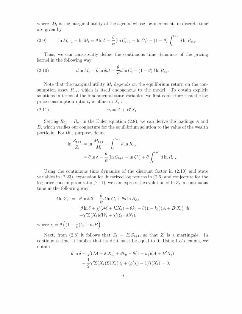
where Mt is the marginal utility of the agents, whose log-increments in discrete timeare given by
(2.9) lnMt+1 − lnMt = θ ln δ − θ
ψ(lnCt+1 − lnCt) − (1 − θ)
∫ t+1
t
d lnRc,s.
Thus, we can consistently define the continuous time dynamics of the pricingkernel in the following way:
(2.10) d lnMt = θ ln δdt− θ
ψd lnCt − (1 − θ)d lnRc,t.
Note that the marginal utility Mt depends on the equilibrium return on the con-sumption asset Rc,t, which is itself endogenous to the model. To obtain explicitsolutions in terms of the fundamental state variables, we first conjecture that the logprice-consumption ratio vt is affine in Xt :
(2.11) vt = A +B′Xt.
Setting Ri,t = Rc,t in the Euler equation (2.8), we can derive the loadings A andB, which verifies our conjecture for the equilibrium solution to the value of the wealthportfolio. For this purpose, define
lnZt+1
Zt= ln
Mt+1
Mt
+
∫ t+1
t
d lnRc,s
= θ ln δ − θ
ψ(lnCt+1 − lnCt) + θ
∫ t+1
t
d lnRc,s.
Using the continuous time dynamics of the discount factor in (2.10) and statevariables in (2.23), expression for linearized log returns in (2.6) and conjecture for thelog price-consumption ratio (2.11), we can express the evolution of lnZt in continuoustime in the following way:
d lnZt = θ ln δdt− θ
ψd lnCt + θd lnRc,t
= [θ ln δ + χ′(M + KXt) + θk0 − θ(1 − k1)(A+B′Xt)] dt
+χ′Σ(Xt)dWt + χ′(ξt · dNt),
where χ = θ(
(1 − 1ψ)δc + k1B
)
.
Next, from (2.8) it follows that Zt = EtZt+1, so that Zt is a martingale. Incontinuous time, it implies that its drift must be equal to 0. Using Ito’s lemma, weobtain
θ ln δ + χ′(M + KXt) + θk0 − θ(1 − k1)(A +B′Xt)
+1
2χ′Σ(Xt)Σ(Xt)
′χ+ ((χ) − 1)′l(Xt) = 0.
9

Matching the coefficients on a constant and Xt, we obtain the following equationsfor A and B :
0 = K′χ− θ(1 − k1)B +1
2χ′Hχ+ l′1((χ) − 1),(2.12)
0 = θ(ln δ + k0 − (1 − k1)A) + M′χ+1
2χ′hχ+ l′0((χ) − 1).(2.13)
In general, these equations can yield multiple solutions to A and B. In our nu-merical example, we generalize the criterion in Tauchen (2005) and select the rootwhich ensures the non-explosiveness of the system as the contributions of stochas-tic volatility and jump components converge to zero. An alternative approach is tochoose an ”economically reasonable” solution which responds intuitively to modeland preference parameters. We will provide more discussion in the empirical sectionof the paper.
Similar to Bansal, Kiku and Yaron (2006), we solve for the linearization constantsk0 and k1 as part of the equilibrium solution of the model. From (2.11)
(2.14) E(vt) = A+B′µX ,
where µX is the vector with ith component
µX,i =
E(Xi) if E(Xi) exists,
0 otherwise.
Expanding k0 in terms of k1 we can show that
k0 + (k1 − 1)A = k0 − (1 − k1)(E(vt) − B′µX)
= − ln k1 + (1 − k1)B′µX .
(2.15)
Plugging this expression into (2.12), we obtain that the linearization coefficient k1
satisfies the following non-linear equation:
(2.16) θ ln k1 = θ (ln δ + (1 − k1)B′µX) + M′χ+
1
2χ′hχ + l′0((χ) − 1).
Given the parameters of the model, we numerically iterate on k1 in the formula abovestarting from the initial value δ, which is the exact the solution for k1 when ψ = 1. Forthe parameter values we consider, the algorithm converges very fast, in 2-5 iterations.
Using the equilibrium solution to the return on wealth portfolio, the evolution ofthe log pricing kernel can now be written in terms of the economic fundamentals:
d lnMt = θ ln δdt− θ
ψd lnCt + (θ − 1)d lnRc,t
= (θ ln δ − (θ − 1) ln k1 + (θ − 1)(k1 − 1)B′(Xt − µX)) dt− λ′dXt,
(2.17)
10
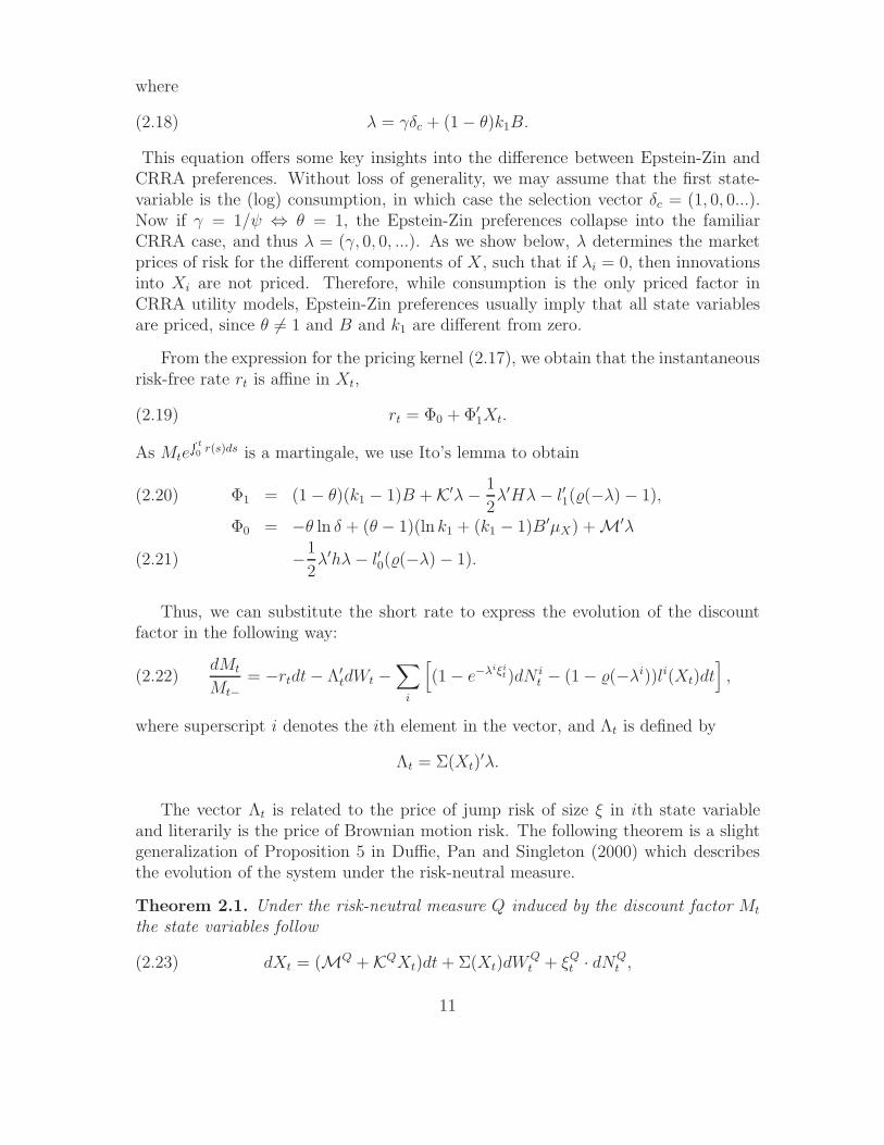
where
(2.18) λ = γδc + (1 − θ)k1B.
This equation offers some key insights into the difference between Epstein-Zin andCRRA preferences. Without loss of generality, we may assume that the first state-variable is the (log) consumption, in which case the selection vector δc = (1, 0, 0...).Now if γ = 1/ψ ⇔ θ = 1, the Epstein-Zin preferences collapse into the familiarCRRA case, and thus λ = (γ, 0, 0, ...). As we show below, λ determines the marketprices of risk for the different components of X, such that if λi = 0, then innovationsinto Xi are not priced. Therefore, while consumption is the only priced factor inCRRA utility models, Epstein-Zin preferences usually imply that all state variablesare priced, since θ 6= 1 and B and k1 are different from zero.
From the expression for the pricing kernel (2.17), we obtain that the instantaneousrisk-free rate rt is affine in Xt,
(2.19) rt = Φ0 + Φ′
1Xt.
As MteR t0 r(s)ds is a martingale, we use Ito’s lemma to obtain
Φ1 = (1 − θ)(k1 − 1)B + K′λ− 1
2λ′Hλ− l′1((−λ) − 1),(2.20)
Φ0 = −θ ln δ + (θ − 1)(ln k1 + (k1 − 1)B′µX) + M′λ
−1
2λ′hλ− l′0((−λ) − 1).(2.21)
Thus, we can substitute the short rate to express the evolution of the discountfactor in the following way:
(2.22)dMt
Mt−
= −rtdt− Λ′
tdWt −∑
i
[
(1 − e−λiξit)dN i
t − (1 − (−λi))li(Xt)dt]
,
where superscript i denotes the ith element in the vector, and Λt is defined by
Λt = Σ(Xt)′λ.
The vector Λt is related to the price of jump risk of size ξ in ith state variableand literarily is the price of Brownian motion risk. The following theorem is a slightgeneralization of Proposition 5 in Duffie, Pan and Singleton (2000) which describesthe evolution of the system under the risk-neutral measure.
Theorem 2.1. Under the risk-neutral measure Q induced by the discount factor Mt
the state variables follow
(2.23) dXt = (MQ + KQXt)dt+ Σ(Xt)dWQt + ξQt · dNQ
t ,
11
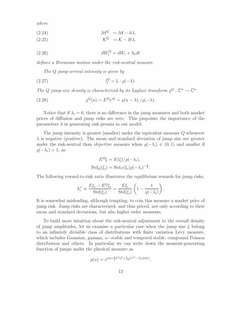
where
MQ = M− hλ,(2.24)
KQ = K −Hλ.(2.25)
(2.26) dWQt = dWt + Λtdt
defines a Brownian motion under the risk-neutral measure.
The Q jump-arrival intensity is given by
(2.27) lQt = lt · (−λ).
The Q jump-size density is characterized by its Laplace transform Q : Cn → Cn
(2.28) Q(u) = EQeuξ = (u− λ)./(−λ).
Notice that if λi = 0, there is no difference in the jump measures and both marketprices of diffusion and jump risks are zero. This pinpoints the importance of theparameters λ in generating risk premia in our model.
The jump intensity is greater (smaller) under the equivalent measure Q wheneverλ is negative (positive). The mean and standard deviation of jump size are greaterunder the risk-neutral than objective measure when (−λi) ∈ (0, 1) and smaller if(−λi) > 1, as
EQξ = E(ξ)/(−λi),StdQ(ξi) = StdP (ξi)(−λi)−
12 .
The following reward-to-risk ratio illustrates the equilibrium rewards for jump risks,
ΛJi ≡ Eξi − EQξi
Std(ξi)=
EξiStd(ξi)
(
1 − 1
(−λi)
)
.
It is somewhat misleading, although tempting, to coin this measure a market price ofjump risk. Jump risks are characterized, and thus priced, not only according to theirmean and standard deviations, but also higher order moments.
To build more intuition about the risk-neutral adjustment to the overall densityof jump amplitudes, let us examine a particular case when the jump size ξ belongto an infinitely divisible class of distributions with finite variation Levy measure,which includes Gaussian, gamma, α−stable and tempered stable, compound Poissondistribution and others. In particular we can write down the moment-generatingfunction of jumps under the physical measure as
(u) = eµu+ 12σ2u2+
RR
(eux−1)ω(dx),
12
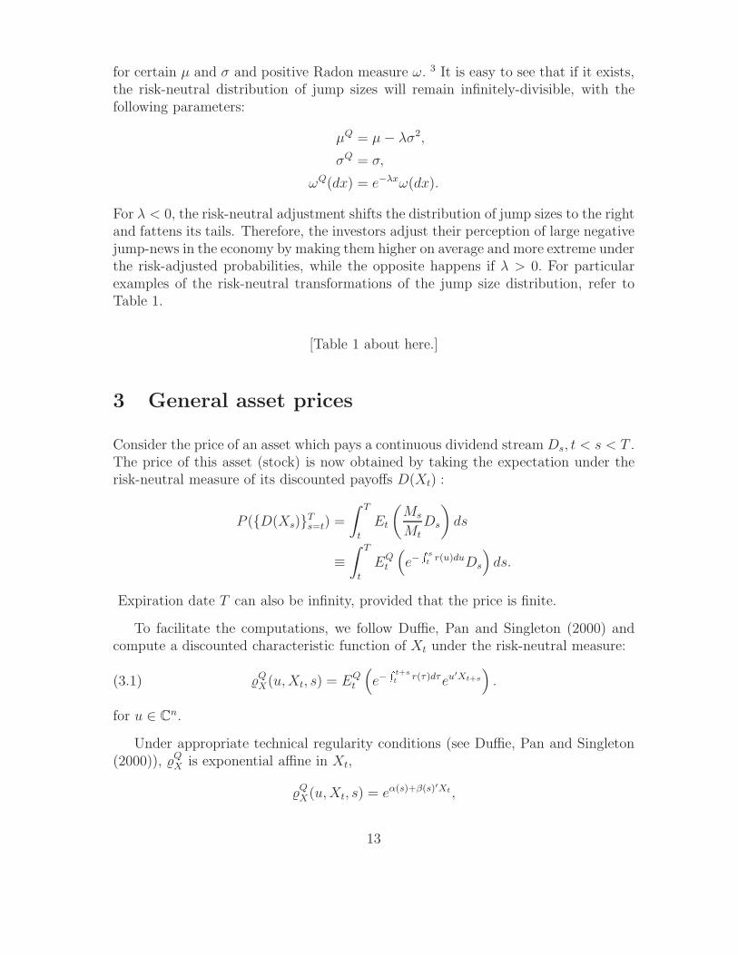
for certain µ and σ and positive Radon measure ω. 3 It is easy to see that if it exists,the risk-neutral distribution of jump sizes will remain infinitely-divisible, with thefollowing parameters:
µQ = µ− λσ2,
σQ = σ,
ωQ(dx) = e−λxω(dx).
For λ < 0, the risk-neutral adjustment shifts the distribution of jump sizes to the rightand fattens its tails. Therefore, the investors adjust their perception of large negativejump-news in the economy by making them higher on average and more extreme underthe risk-adjusted probabilities, while the opposite happens if λ > 0. For particularexamples of the risk-neutral transformations of the jump size distribution, refer toTable 1.
[Table 1 about here.]
3 General asset prices
Consider the price of an asset which pays a continuous dividend stream Ds, t < s < T .The price of this asset (stock) is now obtained by taking the expectation under therisk-neutral measure of its discounted payoffs D(Xt) :
P (D(Xs)Ts=t) =
∫ T
t
Et
(
Ms
Mt
Ds
)
ds
≡∫ T
t
EQt
(
e−R str(u)duDs
)
ds.
Expiration date T can also be infinity, provided that the price is finite.
To facilitate the computations, we follow Duffie, Pan and Singleton (2000) andcompute a discounted characteristic function of Xt under the risk-neutral measure:
(3.1) QX(u,Xt, s) = EQt
(
e−R t+st
r(τ)dτeu′Xt+s
)
.
for u ∈ Cn.
Under appropriate technical regularity conditions (see Duffie, Pan and Singleton(2000)), QX is exponential affine in Xt,
QX(u,Xt, s) = eα(s)+β(s)′Xt ,
13

where α(s) and β(s) satisfy complex-valued ordinary differential equations
β = −Φ1 + KQ′
β +1
2β ′Hβ + lQ1
′ (
Q(β) − 1)
,
α = −Φ0 + MQ′
β +1
2β ′hβ + lQ0
′ (
Q(β) − 1)
,(3.2)
subject to boundary conditions β(0) = u, α(0) = 0.
In particular, setting u = 0 we immediately obtain that the yield on a discountbond with s periods to maturity is given by,
y(Xt, s) = −1
s(α(s) + β(s)′Xt) ,
where α and β solve the ODEs in (3.2) with boundary condition β(0) = α(0) = 0.Note that as the initial values for α and β are real and the risk-neutral mgf of jumpdistribution is assumed to exist (i.e. take real values), the solution to the yield curveis guaranteed to be real as well.
3.1 Dividend Paying Assets
Consider an asset which dividend stream can be expressed as a linear function of thestate variables,
d lnDt = δ′ddXt.
From the discussion in the previous section, the price of an asset which pays a per-petual dividend Dt, if it exists, is given by
Pt(Xt) =∫
∞
0QX(δd, Xt, s)ds
=∫
∞
0eα(s)+β(s)′Xtds,(3.3)
where α and β satisfy the ODEs in (3.2) subject to β(0) = δd and α(0) = 0.
Equation (3.3) gives the exact equilibrium price-dividend ratio when the stockpays a perpetual dividend. To build more intuition about the model, we consideran approximate equilibrium solution which is obtained, as for the consumption asset,through the log-linearization of returns. It is straightforward to show that in thiscase, the equilibrium price-dividend ratio is exponential linear,
(3.4) Pt = Dt exp(Ad +B′
dXt),
where the coefficients Ad and Bd satisfy
(3.5) K′χd + (θ − 1)(k1 − 1)B + (k1,d − 1)Bd +1
2χ′
dHχd + l′1 [ρ(χd) − 1] = 0
14

and
(3.6) θ ln δ − (θ − 1) (ln k1 + (k1 − 1)B′µX) − (ln k1,d + (k1,d − 1)B′
dµX)
+ M′χd +1
2χ′
dhχd + l0 [ρ(χd) − 1] = 0,
for
χd = δd + k1,dBd − λ,(3.7)
and k1,d is the log-linearization coefficient for a dividend return. As before, we cansolve the equations above for Bd and k1,d, and then obtain an intercept Ad from thechain of equalities
Ad +B′
dµX = E lnPtDt
= lnk1,d
1 − k1,d.
(3.8)
The first equality follows from the conjectured solution for the price-dividend ratio,while the second one comes from the log-linearization procedure.
The main advantage of the formulae presented in this section is that we can obtainan exponential affine representation of the equilibrium stock price dynamics, subjectto our log-linearization of returns. This facilitates the computations of option prices,as illustrated next.
3.2 Option Pricing
Lewis (2000) and Carr and Madan (1999) discuss methods for computing optionprices from the characteristic function of the underlying stock price. In the followingwe adapt the formula in Lewis (2000) to our setting.
The price of a European call option is a function of the state variables Xt, strikeprice K and maturity of an option s:
(3.9) C(Xt, K, s) = EQt
[
e−R t+st
rτdτ(
elnPt+s −K)+
]
.
Using the Parseval identity, we obtain that
C(Xt, K, s) = EQt
[
e−R t+st
rτdτ(
elnPt+s −K)+
]
=1
2πEQt
[∫ izi+∞
izi−∞
e−R t+st
rτdτe−iz lnPt+sw(z)dz
]
,(3.10)
15

where the generalized Fourier transform of the payoff function of the option w(z) isequal to,
w(z) =
∫
∞
−∞
eizx (ex −K)+ dx
= − Kiz+1
z2 − iz,
(3.11)
for zi ≡ Im(z) > 1, and identical expression obtains for put options for zi < 0.
If a stock pays a single terminal dividend DT at some date T > s > t or if welog-linearize the returns on a stock which pays dividend continuously, the equilibriumvalue of an asset will be linear in the state variables:
lnPt = Ad + (Bd + δd)′Xt.(3.12)
Using a discounted characteristic function of state variables under the risk-neutralmeasure defined in (3.1), we can rewrite the expression for the option price in thefollowing way:
C(Xt, K, s) = −K 1
2π
∫ izi+∞
izi−∞
e−izAdQX(−z(Bd + δd), Xt, s)Kiz
z2 − izdz.(3.13)
The integration in (3.10) is performed on the intersection of the strips zi > 1for call option or zi < 0 for puts, and the one parallel to the real z−axis. Noticethat (3.10) requires a single numerical integration, which is advantageous relativeto the formulae in the extant literature (e.g. Heston 1993; Bates 1996; Duffie, Panand Singleton 2000) which require two numerical integrations. In addition, thediscounted characteristic function QX is known up to a system of ordinary differentialequations (3.2), which depend on preference, cash flow parameters and maturity ofan option, but do not involve strike price K. In this case, calculating option pricesfor a range of strikes is particularly convenient and fast.
4 The Equilibrium Impact of Volatility Shocks
In an application of our model, we consider an economy in which consumption, div-idends and in the end asset prices, are influenced by a single state variable, whichis the conditional volatility of consumption growth. To this end we assume that logaggregate consumption follows
d lnCt = µdt+√
VtdWc,t,(4.1)
dVt = κV (V − Vt)dt+ σv√
VtdWV,t + ξV dNt,(4.2)
ξV ∼ GA(ν, µV /ν),(4.3)
l(Vt) = l0 + l1Vt.(4.4)
16

The volatility process Vt is driven by the continuous Brownian motion dWV,t as wellas discontinuous process ξV dNt, whose arrival intensity is l(Vt). Our assumptionof Gamma distributed volatility jump sizes allows a fairly heavily tailed jump sizedistribution for small values of the scale parameter ν.
The specification above encompasses a number of stochastic volatility models inthe literature, including square root volatility model of Heston (1993), the exponentialjump diffusion model of Duffie, Pan and Singleton (2000), Eraker (2004), amongothers. By removing the diffusion part, σv = 0, the volatility dynamics reduces to thegamma OU process (l1 = 0 and ν = 1). For a detailed treatment of Non-Gaussian OUprocesses refer to Barndorff-Nielsen and Shephard (2001). Our specification of theconsumption process is a simplification of the Bansal and Yaron (2004) model in thatthe expected log consumption growth is constant. In the Bansal and Yaron (2004)model, the expected consumption growth follows a mean-reverting AR(1) process.Fixing the expected growth rate in our model allows us to focus entirely on theequilibrium effects of stochastic volatility.
The first step in our analysis is to recover expressions for the coefficients A andB in eqns. (2.12) and (2.13). The loading on consumption growth is zero, while the”volatility factor loading” Bv solves(4.5)
0 = −θ [κvk1 + (1 − k1)]Bv+1
2θ2(1− 1
ψ)2 +
1
2θ2k2
1σ2vB
2v + l1
[
(1 − Bvθk1µv/ν)−ν − 1
]
.
This equation admits an explicit solution only in special cases. In particular, ifthere are no state-dependent volatility jumps, l1 = 0, then Bv solves the quadraticequation a + bBv + cB2
v = 0 for a = θ2 12(1 − 1
ψ)2, b = −θ(κv + (1 − k1)), c = θ2κ2
1σ2v .
Tauchen (2005) points out that square root processes for volatility generally producetwo roots for Bv. However, if θ < 0, b is positive, so that only the ”right” root isnon-explosive when a stochastic volatility parameter σv converges to 0. By includingstate-dependent volatility jumps, we generally have more than two roots. In thecase where the volatility is driven by pure jumps (σv = 0) and volatility jumps areexponentially distributed (ν = 1), we can recover another quadratic equation for Bv,and we can use a similar argument to select the non-explosive solution when thejump contribution is converging to zero. When σv and l1 are not zero, for reasonableparameter values we typically obtain two real solutions for Bv, and we choose the”right” root near the one implied by a quadratic equation above.
17
Given the solution to Bv, we recover the dynamics of the state variables underthe risk-neutral measure:
d lnCt = (µ− γVt)dt+√
VtdWQc,t(4.6)
dVt = κV (V − Vt)dt− λvσ2vVtdt+ σv
√
VtdWQV,t + ξQV dN
Qt(4.7)
ξQV ∼ GA(ν,µv
ν + λvµv)(4.8)
lQ(Vt) = (1 +λvµvν
)−νl(Vt),(4.9)
where λv = (1 − θ)k1Bv denotes the price of the variance shock.
This process is well defined whenever ν > λvµv, which places implicit restrictionson the permissible preference parameters. If this holds and the market price of volatil-ity risk is negative, then both jump sizes and arrival intensity are greater under therisk-neutral measure,
EQξV > EP ξV ,
V arQξV > V arP ξV ,
lQ(Vt) > l(Vt).
In the case of exponentially distributed jump sizes, ν = 1, and jump size distribu-tion as well as jump intensity are scaled by a constant (1 + λvµv)
−1, which is greaterthan one whenever ψ > 1, γ > 1. This offers a very simple and intuitive adjustmentfrom the objective to the risk-neutral measure.
4.1 Dividends
We consider a stock whose perpetual dividend stream follows
d lnDt = φd lnCt + σd√
VtdWd,t,
where the parameter φ can be interpreted as a ”consumption leverage” parameteror the OLS slope coefficient obtained by regressing d lnDt on d lnCt. Wheneverφ > 1, we can think of the corporate dividends as being a levered position on totalconsumption output. The idea of dividends as a levered position on consumption isuseful in reconciling the low consumption volatility with high volatilities of corporateearning and dividends. The term σd
√VtdWd,t represents asset specific noise which is
not priced in equilibrium.
It is straightforward to recover an exact pricing formula for the price of a stock,as in equation (3.3). However, in order to recover exponential affine stock price
18
dynamics, we log-linearize stock returns, so that the equilibrium price-dividend ratiocan be written as exp(Ad +B′
d,vVt). Equations (3.5) become
(4.10) − κv [(θ − 1)k1Bv + k1,dBd,v)] − (θ − 1)(1 − k1)Bv − (1 − k1,d)Bd,v
+1
2
[
(γ − φ)2 + σ2d + σ2
v ((θ − 1)k1Bv + k1,dBd,v)2]
+ l1
[
(
1 − µv(θ − 1)k1Bv
ν− µvk1,dBd,v
ν
)
−ν
− 1
]
= 0,
which can be solved for Bd,v with similar caveats about multiple roots as in theprevious section.
The dividend process follows
d lnDt = φd lnCt + σd√
VtdWQd,t
= φ(µ− γVt)dt+ φ√
VtdWQc,t + σd
√
VtdWQd,t
(4.11)
under the risk-neutral measure. It is now straightforward to show that the stockprice, which is given by lnPt = lnDt + (A+Bd,vVt), evolves according to
(4.12) d lnPt =[
φ(µ− γVt) +Bd,v(κv(V − Vt) − λvσ2vVt)
]
dt
+ σd√
VtdWQd,t + φ
√
VtdWQc,t +Bd,vσv
√
VtdWQv,t +Bd,vξ
QV dN
Qt .
under the risk-neutral measure. In particular, the variation in stock price is generatedby the Brownian motion shocks in dividends, consumption and market volatility aswell as variance jumps. For a reasonable calibration of parameter values, the model-implied stock price volatility is greater than the consumption volatility Vt. In fact,it is easy to generate 15 − 20% stock price volatility while keeping the aggregateconsumption growth variation close to the historical estimates of 2 − 3%. Therefore,our model can account for an excessive volatility of financial variables relative to theeconomic fundamentals.
As the conditional variance of log price is proportional to Vt, the conditionalcorrelation between log price and its variance is given by Corrt(d lnPt, dVt). Thelatter is equal to
(4.13) Corrt(d lnPt, dVt) = Bd,v
√
σ2vVt + µ2
vν−1(l0 + l1Vt)
Vt(σ2d + φ2 +B2
d,vσ2v) +B2
d,vµ2vν
−1(l0 + l1Vt),
where l0, l1 and µv can be under either the physical or risk-neutral measure. Thus,the correlations of the stock price with volatility are different under the objective Pand risk-neutral measure Q. The difference in P and Q correlation is driven by themagnitude of the jump risk premium. In our model, the jump risk premium increases
19
uniformly in the risk aversion parameter γ. Thus, larger values of γ generate a largerdispersion in the correlation for the two measures. This effect is illustrated in Figure4.1.
[Figure 1 about here.]
Notice that the correlation is increasing (in absolute value) in the parameter Bd,v.This parameter typically takes on negative values for ψ, γ > 1. This implies thatthe correlation in (4.13) approaches negative one for large values of γ and ψ. Fig-ure 4.1 illustrates this effect. The figure also shows that the correlation under boththe objective and the risk-neutral measures becomes more negative when risk aver-sion increases. The correlation is less negative for all values of γ when the valueof the idiosyncratic dividend noise term, σd, is higher, illustrating that individualstocks (which contain a larger fraction of idiosyncratic noise) exhibit less pronouncedvolatility/stock price correlation than do equity indices.
The negative sign shows that increased macroeconomic uncertainty leads to lowerequilibrium stock valuations. Correlations are higher in absolute value under therisk-neutral measure, and the difference between the two measures increases with therisk aversion coefficient. This is an important observation, because researchers whoattempt to fit reduced form no-arbitrage models to option price data often find thatthe magnitude of the stock/price volatility correlation well exceeds the correlationsestimated from the actual stock price and volatility estimates. For example, Bakshi,Cao and Chen (1997) calibrate jump diffusion models and find option implied corre-lations in the -0.6 to - 0.8 range. This is generally outside the range found in returnsdata.
Andersen, Benzoni and Lund (2002) estimate the correlation to be in the -0.5 to-0.6 range. Eraker, Johannes and Polson (2003) estimate it to be in the −0.4 to −0.5range. Eraker (2004) fits various no-arbitrage jump diffusion models to both returnsdata and joint data on options and returns and finds that the correlations are greaterin magnitude when option data is included. A difference of about ten percentagepoints in the P and Q correlations is consistent with a risk aversion, γ, of about ninein our model.
The equity premium in our economy is
(4.14)1
dtEtd lnRd,t − rt = (γφ+ λvk1,dBd,vσ
2v −
1
2(σ2
d + φ2 + k21,dB
2d,vσ
2v))Vt+
(k1,dBd,vµv + (−λv) − (k1,dBd,v − λv)) l(Vt).
The first bracket contains a standard CRRA risk premium γφVt which will be presentin a model with no jumps or time-varying stochastic volatility. The second component,λvk1,dBd,vσ
2vVt, captures the compensation for ”small” volatility shocks dWV,t, while
20

the third term gives an (unimportant) quadratic variation adjustment due to the factthat we work with log, rather than level returns. In the same way, the second bracketcontains the risk premium due to ”large” volatility jumps dNt and the correspondingIto’s adjustment due to jumps in log returns.
With power utility preferences, expected excess returns do not contain the com-pensation for Brownian and jump volatility shocks. On the other hand, the volatilityand jump compensation terms could be large in our model if Bd,v and λv are large.While a careful estimation of model parameters is beyond the scope of this paper, itis interesting to note that the parameter values used to generate the implied volatil-ity graphs reported below generate an equity premium that ranges between one andtwelve percent per annum. Thus, our model could potentially resolve the equity pre-mium puzzle of Mehra and Prescott (1985). We note here that large equity premiumand low risk-free rates is a well documented feature of long run risk models. Eraker(2006) studies a three factor model in which the equity premium puzzle can be re-solved with small values of the risk aversion parameter γ. The presence of volatilityjumps in this model significantly increases the equity premium. It is noticeable thatour model can generate large equity premium even without the ”long run risk” factorthat captures time-variation in expected consumption growth, as is the case in theBansal and Yaron (2004) and Eraker (2006) models.
4.2 Price Patterns
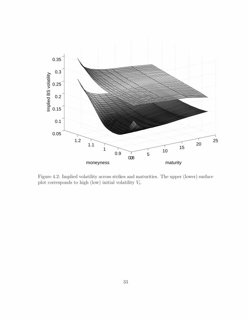
In the following we discuss key properties of option prices computed in our model.The standard measure of empirical patterns in option data is the options impliedvolatility. It is well known that the implied volatility of index options is convex overdifferent strikes. To examine if our model can generate similar patterns, we computeimplied volatilities by equating the theoretical model prices to the ones in the Black& Scholes model using our model solutions for the dividend yields and interest rates.
In Figure 4.2 we plot the implied volatility as a function of the strike price andmaturity. The two surface plots are generated for low and high initial values of thevolatility Vt. The implied volatility patterns are fairly typical of those computed inno-arbitrage models which feature high negative correlation between volatility shocksand prices. The implied volatility has a more pronounced U shape at short maturities,and flattens out at the long end. Evidence of negative skewness is evident even forlong maturity contracts.
[Figure 2 about here.]
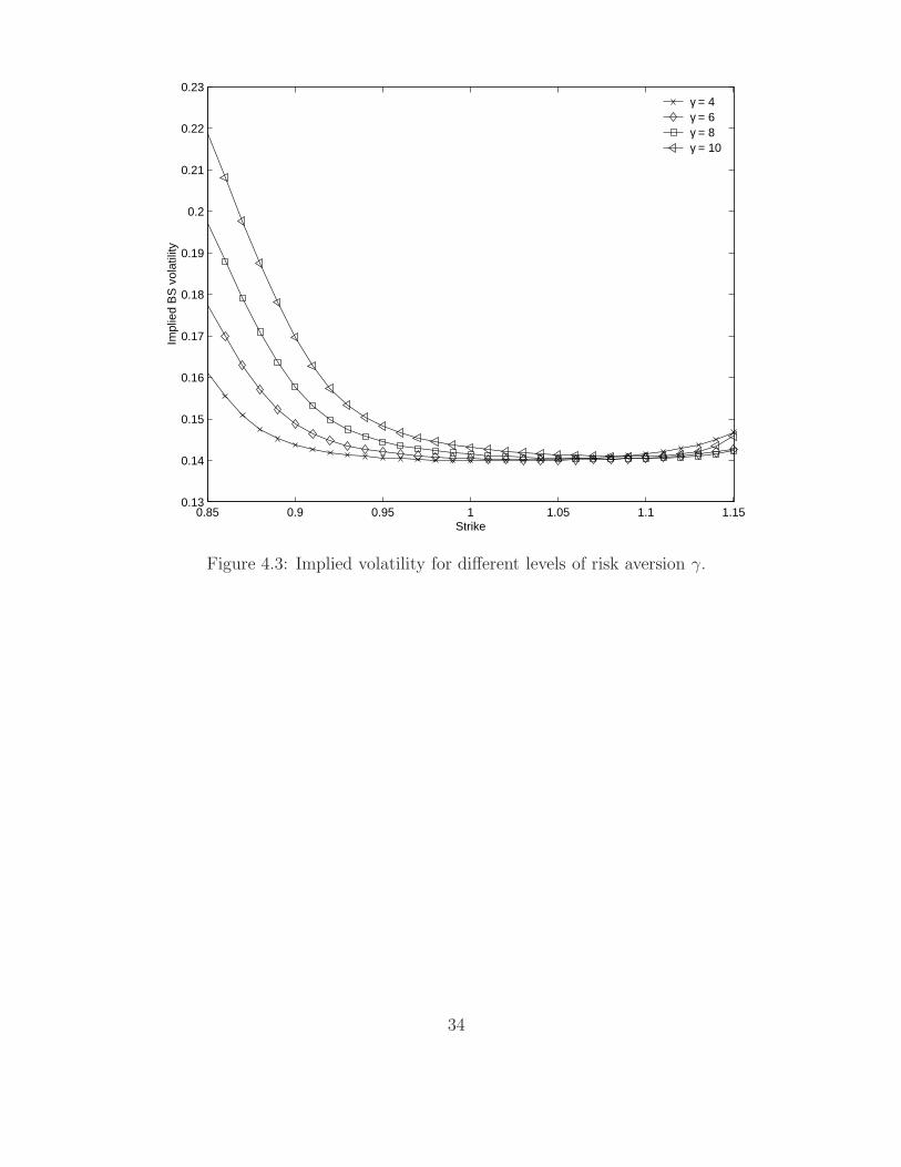
Figure 4.3 depicts the implied volatility of our theoretical model prices computedover different values of risk aversion γ and with a fixed value of ψ = 4. There are two
21

main effects of increasing the level of risk aversion. First, the stock prices becomemore volatile on average. This is reflected by an upward shift in implied volatility forhigher values of γ. Second, and more interesting, the convexity of the curve is muchmore pronounced for higher values of γ, reflecting a more heavily tailed equilibriumstock price distribution. Jumps to the volatility process always result in (negative)jumps in the stock price, as can be seen from equation (4.12). The negative pricereactions to a jump in volatility can be significant, as evidenced by the increasingprices of far out-of-the-money put options in Figure 4.3. Therefore, endogenizing thestock price in an economy where the volatility may increase suddenly can explain thehigh crash insurance premiums offered by out-of-the-money put options.
[Figure 3 about here.]
Does CRRA utility deliver implied volatility graphs that mimic those of the gen-eral Epstein-Zin model? Recall that the CRRA model obtains as a special case byimposing the constraint ψ = 1/γ. We impose this condition in computing impliedvolatilities in figure 4.4. The main difference between the two equilibrium speci-fications is that CRRA model produces implied volatility curves that imply posi-tive conditional skewness in the risk-neutral stock price distribution, as can be seenfrom the fact that contracts with high strikes carry a higher premium. This positiveskewness is attributable to the fact that the parameter Bd,v is positive, indicatinga positive volatility-return correlation in 4.13. For Epstein-Zin preferences, Bd,v isnegative, which yields a negative volatility-return correlation and thus a negativelyskewed stock price density. Thus, Epstein-Zin based equilibrium option prices tend togenerate implied volatility curves that are consistent with those observed empirically.
[Figure 4 about here.]
It is possible to generate very steep equilibrium implied volatility curves in ourexample model. Recall that the parameter ν determines the tail-behavior of thevolatility jump sizes, and a small value of ν leads to heavier tails. Figure 4.5 illustratesthe effect of changing ν. The impact of out-of-the-money puts is significant, and pricesincrease uniformly with lower values of ν. The case where ν = 0.15 illustrates thatthe possibility of a very severe jump in volatility has a dramatic effect on the price ofOTM puts.
[Figure 5 about here.]
Our discussion so far has mostly been relevant in the context of options written onan index of stocks. Stock indices, unlike individual equities, are characterized by the
22

fact that the risks are almost entirely systematic. In our model this is captured by asmall value of σd (we used 0.2 in our preceding discussion). Figure 4.6 illustrates theeffect of increasing idiosyncratic risk, σd, on option prices. While the overall impliedvolatility increases, higher values of σd significantly diminish conditional skewnessand kurtosis as can be seen from an almost flat implied volatility curve. Increasingσd in our model thus has an effect of just adding Gaussian noise to the stock priceprocess. Our model can easily be augmented to allow for company specific dividendjumps. This would generate additional kurtosis, and thus additional convexity inimplied volatilities of individual stock options.
[Figure 6 about here.]
5 Concluding Remarks
Affine class constitutes a significant and important class of asset pricing models.Affine models are typically derived under assumptions of no-arbitrage, which offersa limited ability for economic interpretation of the market prices of risks that linkthe objective probability measure with the risk-neutral pricing measure. Our papersuggests a way to remedy this by constructing a pricing kernel which is based ongeneralized preferences of Epstein and Zin (1989). Importantly, our framework offersa convenient way to link the two measures in the presence of diffusion risks and jumprisks. All risk premia computations in our model are done through the specification ofthe three preference parameters (δ, ψ and γ). Since market prices of risk are explicitfunctions of these three parameters, our model framework offers a more parsimoniousway to compute equilibrium prices than the usual affine no-arbitrage models whichdo not restrict market prices of risk.
We set up an example model with only one state variable, variance of consumptiongrowth driven by Brownian motion shocks and Poisson jumps, and study the equi-librium effects on the equity and option prices. Our model endogenously generatesa negative correlation between shocks to the volatility process and the equilibriumstock prices. The compensation for the variance shocks is sizeable and can help toaccount for a high expected equity return relative to the risk-free rate. The impliedvolatilities are U shaped, with significantly higher prices for out-of-the-money puts;the smile flattens out with a decrease in the risk aversion coefficient. These effectscan not be captured in traditional power utility models.
It is straightforward to include additional state variables into our framework, suchas time-varying expected consumption growth, inflation, multiple volatility and jumpintensity processes, etc. The model can also be confronted with macro and financialdata; there are several possible empirical strategies for identification and estimation
23

of the preference and cash flow dynamics parameters and evaluation of the model inand out of sample. We leave the issues of more elaborate models and empirical fit fora future research.
24

A Log-linearization in Continuous Time
Let d lnRt heuristically denote the continuous time log return so that∫ t+1
td lnRs
define the return over the interval (t, t+ 1]. The Campbell-Shiller approximation tothe discrete time return is then
(A.1)
∫ t+1
t
d lnRs = k0 + k1vt+1 − vt + ∆ lnDt+1
where vt is the log price-dividend ratio, and ∆ lnDt is the dividend growth rate.Equation (A.1) is exactly the same as in discrete time, as we showed in Section 2.
Now rewrite (A.1) as
∫ t+1
t
d lnRs = k0 + k1(vt+1 − vt) − (1 − k1)vt + ∆ lnDt+1
=
∫ t+1
t
k0ds+ k1
∫ t+1
t
dvs − (1 − k1)
∫ t+1
t
vtds+
∫ t+1
t
d lnDs.
From here we define the continuous time return d lnRt :
d lnRt = k0dt+ k1dvt − (1 − k1)vtdt+ d lnDt.(A.2)
For the consumption asset, vt = A+B′Xt and d lnCt = δ′cdXt, so that d lnRc,t is
d lnRc,t = k0dt+ [δc + κ1B]′dXt − (1 − k1)(A+B′Xt)dt.(A.3)
Similar decomposition holds for a log return on a dividend asset d lnRd,t.
25

References
Aase, K. (2002): Equilibrium Pricing in the Presence of Cumulative Dividends Fol-lowing a Diffusion, Mathematical Finance 12, 173-198.
Andersen, T. G., L. Benzoni, and J. Lund (2002): An Empirical Investigation ofContinuous-Time Models for Equity Returns, Journal of Finance 57, 1239-1284.
Bakshi, G., C. Cao, and Z. Chen (1997): Empirical Performance of Alternative OptionPricing Models, Journal of Finance 52, 2003-2049.
Bansal, R. (2007): Long Run Risks and Financial Markets, Working paper, DukeUniversity.
Bansal, R., V. Khatchatrian, and A. Yaron (2005): Interpretable Asset Markets,European Economic Review 49, 531-560.
Bansal, R., D. Kiku, and A. Yaron (2006): Risks for the Long Run: Estimation andInference, Working paper, Duke University.
Bansal, R., and I. Shaliastovich (2007): Risk and Return in Bond, Currency andEquity Markets, Working paper.
Bansal, R., and A. Yaron (2004): Risks for the Long Run: A Potential Resolution ofAsset Pricing Puzzles, Journal of Finance 59, 1481-1509.
Barillas, F., L. Hansen, and T. Sargent (2006): Reinterpreting a Graph (and a Pa-rameter) of Tallarini, Working paper.
Barndorff-Nielsen, O. E., and N. Shephard (2001): Non-Gaussian Ornstein-Uhlenbeck-Based Models and Some of Their Uses in Financial Economics, Journal of Royal
Statistical Society 63, 167-241.
Bates, D. S. (1996): Jump and Stochastic Volatility: Exchange Rate Processes Im-plicit in Deutsche Mark Options, Review of Financial Studies 9, 69-107.
Bates, D.S. (2000): Post-87 Crash fears in S&P 500 Futures Options, Journal of
Econometrics 94, 181-238.
Benzoni, L., P. Collin-Dufresne, and R. S. Goldstein (2005): Can Standard Prefer-ences Explain the Prices of Out-of-the-Money S&P 500 Put Options? Working paper,University of Minnesota.
Campbell, J. (1993): Intertemporal Asset Pricing without Consumption Data, Amer-
ican Economic Review 83, 487-512.
Campbell, J. Y., A.W. Lo, and A. C. Mackinlay (1997): The Econometrics of Finan-
cial Markets. Princeton, N.J.: Princeton University Press.
26
Campbell, J. Y., and R. J. Shiller (1988): Stock Prices, Earnings and Expected Div-idends, Journal of Finance 43, 661-676.
Carr, P., H. Geman, D. Madan, and M. Yor (2003): Stochastic Volatility for LevyProcess, Mathematical Finance 13, 345-382.
Carr, P., and D. Madan (1999): Option Pricing and the Fast Fourier Transform,Journal of Computational Finance 2, 61-73.
Chen, H. (2006): Macroeconomic Conditions and the Puzzles of Credit Spreads andCapital Structure, Working paper.
Cont, R., and P. Tankov (2004): Financial Modelling with Jump Processes. London:Chapman & Hall.
Duffie, D., and L. Epstein (1992): Stochastic Differential Utility, Econometrica 60,353-394.
Duffie, D., and R. Kan (1996): A Yield-Factor Model of Interest Rates, Mathematical
Finance 6, 379-406.
Duffie, D., J. Pan, and K. J. Singleton (2000): Transform Analysis and Asset Pricingfor Affine Jump-Diffusions, Econometrica 68, 1343-1376.
Epstein, L. G., and S. E. Zin (1989): Substitution, Risk Aversion, and the TemporalBehavior of Consumption and Asset Returns, Econometrica 57, 937-69.
Eraker, B. (2004): Do Stock Prices and Volatility Jump? Reconciling Evidence fromSpot and Option Prices, Journal of Finance 59, 1367-1403.
Eraker, B. (2006): Affine General Equilibrium Models, Working paper, Duke Univer-sity.
Eraker, B., M. J. Johannes, and N. G. Polson (2003): The Impact of Jumps in Returnsand Volatility, Journal of Finance 53, 1269-1300.
Garcia, R., R. Luger, and E. Renault (2003): Empirical Assessment of an Intertem-poral Option Pricing Model with Latent Variables, Journal of Econometrics 116,49-83.
Hansen, L., and T. Sargent (2006): Fragile Beliefs and the Price of Model Uncertainty,Working paper.
Hansen, L. P., J. Heaton, and N. Li (2004): Consumption Strikes Back, Workingpaper, University of Chicago.
Heston, S. (1993): Closed-Form Solution of Options with Stochastic Volatility withApplication to Bond and Currency Options, Review of Financial Studies 6, 327-343.
27

Hull, J., and A. White (1987): The Pricing of Options with Stochastic Volatilities,Journal of Finance 42, 281-300.
Lewis, A. (2000): Option Valuation under Stochastic Volatility. Finance Press.
Liu, J., J. Pan, and T. Wang (2005): An Equilibrium Model of Rare-Event Premiaand its Implication for Option Smirks, Review of Financial Studies 18, 131-164.
Madan, D., P. Carr, and E. Chang (1998): The Variance Gamma Process and OptionPricing, European Finance Review 2, 79-105.
Maenhout, P. J. (2004): Robust Portfolio Rules and Asset Pricing, Review of Finan-
cial Studies 17, 951-983.
Mehra, R., and E. Prescott (1985): The Equity Premium: A Puzzle, Journal of
Monetary Economics 15, 145-161.
Schroder, M., and C. Skiadas (1999): Optimal Consumption and Portfolio Selectionwith Stochastic Differential Utility, Journal of Economic Theory 89, 68-126.
Shaliastovich, I., and G. Tauchen (2006): Pricing Implications of Stochastic Volatility,Business Cycle Time Change, and Non-Gaussianity, Working paper, Duke University.
Tallarini, T. (2000): Risk-Sensitive Real Business Cycles, Journal of Monetary Eco-
nomics 45(3), 507-532.
Tauchen, G. (2005): Stochastic Volatility in General Equilibrium, Working paper,Duke University.
Weil, P. (1989): The Equity Premium Puzzle and the Risk Free Rate Puzzle, Journal
of Monetary Economics 24, 401-421
28

Notes
1 For robust empirical evidence on the magnitude of the IES and the asset pricingimplications in equity, bond and currency markets refer, for instance, to Bansal,Khatchatrian and Yaron (2005), Eraker (2006) and , Bansal and Shaliastovich (2007).
2Other approximations are possible - see for example Hansen, Heaton and Li(2004), Benzoni, Collin-Dufresne and Goldstein (2005).
3These results apply under certain technical existence and integrability conditions(see, e.g. Cont and Tankov 2004 ).
29

Tables and Figures
30

Name Physical measure Risk-Neutral measure RestrictionsInfinitely Divisible Distributions
Normal (u;µ, σ) = euµ+ 12u2σ2 µQ = µ− λσ2
σQ = σ
Gamma (u; ν, µvν
) = (1 − µvνu)−ν
νQ = νµQv = µvr
ν+λµv
ν, µv > 0u < min( ν
µv, νµv
+ λ)
Tempered Stable (u; c, α, ν) = eνΓ(−α)((c−u)α−cα)
νQ = ναQ = αcQ = c+ λ
α ∈ (0, 1)ν, c > 0u < min(c, c+ λ)
Compound Poisson (u; c, f) = ec
R(eux−1)f(x)dx cQ = c
∫
e−λxf(x)dxfQ(x) = e−λxf(x)/
∫
e−λxf(x)dx
c > 0f(x) is pdf∫
euxf(x)dx < ∞Non-Infinitely Divisible Distributions
Uniform (u; a, b) = eu(b−a)
u(b−a)Q(u; a, b) = eu(b−a)λ
λ−ub > a
Table 1: The risk-neutral adjustment to the jump size distribution.
31

2 3 4 5 6 7 8 9 10−0.8
−0.7
−0.6
−0.5
−0.4
−0.3
−0.2
−0.1
0
0.1
0.2
Risk aversion, γ
Objective measure, σd = 0.2
Risk neutral measure, σd = 0.2
Objective measure, σd = 4
Risk neutral measure, σd = 4
Figure 4.1: Correlation between the innovations in log stock price and market varianceas a function of risk aversion γ.
32
05
1015
2025
0.80.9
11.1
1.2
0.05
0.1
0.15
0.2
0.25
0.3
0.35
maturitymoneyness
Impl
ied
BS
vol
atili
ty
Figure 4.2: Implied volatility across strikes and maturities. The upper (lower) surfaceplot corresponds to high (low) initial volatility Vt.
33
0.85 0.9 0.95 1 1.05 1.1 1.150.13
0.14
0.15
0.16
0.17
0.18
0.19
0.2
0.21
0.22
0.23
Strike
Impl
ied
BS
vol
atili
ty
γ = 4γ = 6γ = 8γ = 10
Figure 4.3: Implied volatility for different levels of risk aversion γ.
34

0.85 0.9 0.95 1 1.05 1.1 1.150.13
0.14
0.15
0.16
0.17
0.18
0.19
0.2
0.21
0.22
0.23
Strike
Impl
ied
BS
vol
atili
ty
γ = 4γ = 6γ = 8γ = 10
Figure 4.4: Implied volatility for different levels of risk aversion γ in the case of CRRAutility.
35

0.85 0.9 0.95 1 1.05 1.1 1.15
0.14
0.16
0.18
0.2
0.22
0.24
0.26
Strike
Impl
ied
BS
vol
atili
ty
ν = 0.15ν = 0.65ν = 1.15ν = 1.65
Figure 4.5: Implied volatility for different levels of volatility jump tail-thickness ν.
36

0.85 0.9 0.95 1 1.05 1.1 1.15
0.14
0.16
0.18
0.2
0.22
0.24
0.26
0.28
Strike
Impl
ied
BS
vol
atili
ty
σd = 0.2
σd = 1
σd = 1.8
σd = 2.6
σd = 3.6
Figure 4.6: Implied volatility for different levels of idiosyncratic risk σd.
37