an equity profile of...
TRANSCRIPT
An Equity Profile of
AlbuquerqueJune 2018
An Equity Profile of Albuquerque PolicyLink and PERE 2
This profile was written by James Crowder Jr.
at PolicyLink; the data, charts, and maps were
prepared by Sheila Xiao, Pamela Stephens,
and Justin Scoggins at PERE; and Rosamaria
Carrillo of PolicyLink assisted with formatting,
editing, and design.
PolicyLink and the Program for Environmental
and Regional Equity (PERE) at the University
of Southern California are grateful to the W.K.
Kellogg Foundation for their generous
support of this project and our long-term
organizational partnership.
We also thank the city of Albuquerque, and
the members of our advisory committee:
James Jimenez from New Mexico Voices for
Children, Dr. Meriah Heredia-Griego from the
University of New Mexico’s Center for
Education Policy Research, Javier Martinez
from the Partnership for Community Action,
Kay Bounkeua from the New Mexico Asian
Family Center, Vanessa Roanhorse, Giovanna
Rossi from Collective Action Strategies, and
Albino Garcia from La Plazita Institute for
insightful guidance and feedback.
Finally, we are grateful to our partners
Dolores Acevedo-Garcia and Erin Hardy at
The diversitydatakids.org Project for allowing
us to include their unique data on child and
family well-being in this series of profiles.
Acknowledgments
Demographics
Economic vitality
Economic Benefits
Implications
Readiness
Connectedness
PolicyLink and PEREAn Equity Profile of Albuquerque
Summary Equity Profiles are products of a partnership
between PolicyLink and PERE, the Program
for Environmental and Regional Equity at the
University of Southern California.
The views expressed in this document are
those of PolicyLink and PERE.
3
Table of contents
Data and methods
Introduction
25
59
9
75
86
4
15
92
95
An Equity Profile of Albuquerque PolicyLink and PERE 4
Summary While the nation is projected to become a people-of-color majority by the year 2044, Albuquerque reached that milestone in the 2000s. Since 1990, Albuquerque has experienced dramatic demographic growth and transformation – driven mostly by an increase in the Latino and Asian or Pacific Islander population. Today, these demographic shifts – including a decrease in the percentage of White residents – persist.
Albuquerque’s diversity is a major asset in the global economy, but inequities and disparities are holding the region back. Albuquerque is the 59th most unequal among the largest 100 metro regions. Since 2000, poverty and working-poverty rates in the region have been consistently higher than the national averages. Racial and gender wage gaps persist in the labor market. Closing racial gaps in economic opportunity and outcomes will be key to the region’s future.
Equitable growth is the path to sustained economic prosperity in Albuquerque. The region’s economy could have been more than $10 billion stronger in 2014 if its racial gaps in income had been closed: a nearly 20 percent increase. By growing good jobs, connecting younger generations with older ones, integrating immigrants into the economy, building communities of opportunity, and ensuring educational and career pathways to good jobs for all, Albuquerque can put all residents on the path toward reaching their full potential, and secure a bright future for the city and region.
PolicyLink and PEREAn Equity Profile of Albuquerque 5
IndicatorsDemographics
17 Race/Ethnicity and Nativity, 2014
17 Latino, Native American, and Asian or Pacific Islander Populations
by Ancestry, 2014
18 Percent Change in People of Color by Census Block Group,
2000 to 2014
19 Racial/Ethnic Composition, 1980 to 2014
19 Composition of Net Population Growth by Decade, 1980 to
2014
20 Growth Rates of Major Racial/Ethnic Groups, 2000 to 2014
20 Share of Net Growth in Black and Latino Population by Nativity,
2000 to 2014
21 Racial/Ethnic Composition by Census Block Group, 1990 and
2014
22 Racial/Ethnic Composition, 1980 to 2050
23 Percent People of Color (POC) by Age Group, 1980 to 2014
23 Median Age by Race/Ethnicity, 2014
24 The Racial Generation Gap in 2014: 100 Largest Cities, Ranked
Economic vitality
27 Cumulative Job Growth, 1979 to 2014
27 Cumulative Growth in Real GRP, 1979 to 2014
28 Unemployment Rate, 1990 to 2015
29 Cumulative Growth in Jobs-to-Population Ratio, 1979 to 2014
30 Labor Force Participation Rate by Race/Ethnicity, 1990 and 2014
30 Unemployment Rate by Race/Ethnicity, 1990 and 2014
31 Unemployment Rate by Race/Ethnicity, 2014
32 Unemployment Rate by Census Tract, 2014
33 Gini Coefficient, 1979 to 2014
34 Real Earned Income Growth for Full-Time Wage and Salary
Workers Ages 25-64, 1979 to 2014
35 Median Hourly Wage by Race/Ethnicity, 2000 and 2014
36 Households by Income Level, 1979 and 2014
37 Racial Composition of Middle-Class Households and All
Households, 1979 and 2014
38 Poverty Rate, 1980 to 2014
PolicyLink and PEREAn Equity Profile of Albuquerque 6
IndicatorsEconomic vitality (continued)
38 Working Poverty Rate, 1980 to 2014
39 Poverty Rate by Race/Ethnicity, 2014
39 Working Poverty Rate by Race/Ethnicity, 2014
40 Percent of the Population Below 200 Percent of Poverty, 1980
to 2014
41 Unemployment Rate by Educational Attainment and Race/Ethnicity,
2014
42 Median Hourly Wage by Educational Attainment and
Race/Ethnicity, 2014
43 Unemployment Rate by Educational Attainment, Race/Ethnicity,
and Gender, 2014
43 Median Hourly Wage by Educational Attainment, Race/Ethnicity,
and Gender, 2010-2014
44 Growth in Jobs and Earnings by Industry Wage Level, 1990 to 2015
45 Industries by Wage Level Category in 1990 and 2015
46 Industry Employment Projections, 2014-2024
47 Industry Employment Projections, 2014-2024
49 Industry Strength Index
50 Occupation Opportunity Index
52 Occupation Opportunity Index: Occupations by Opportunity Level
for Workers with a High School Diploma or Less
53 Occupation Opportunity Index: Occupations by Opportunity
Level for Workers with More Than a High School Diploma but Less
Than a Bachelor’s Degree
54 Occupation Opportunity Index: All Levels of Opportunity for
Workers with a Bachelor’s Degree or Higher
55 Opportunity Ranking of Occupations by Race/Ethnicity, All Workers
56 Opportunity Ranking of Occupations by Race/Ethnicity, Workers
with Low Educational Attainment
57 Opportunity Ranking of Occupations by Race/Ethnicity, Workers
with Middle Educational Attainment
58 Opportunity Ranking of Occupations by Race/Ethnicity, Workers
with High Educational Attainment
Readiness
61 Educational Attainment by Race/Ethnicity, 2014
62 Public or Private Pre-Kindergarten or Kindergarten Attendance,
2010 to 2014
62 Share of Students in Grades 3-8 (in public and charter schools)
Achieving Proficient on State Exams in Reading, Math, Science, and
Social Studies (Combined), 2014-2015
PolicyLink and PEREAn Equity Profile of Albuquerque 7
IndicatorsReadiness (continued)
63 Share of Working-Age Population with an Associate’s Degree or
Higher by Race/Ethnicity and Nativity, 2014, and Projected Share of
Jobs that Require an Associate’s Degree or Higher, 2020
64 Percent of the Population with an Associate’s Degree or Higher
in 2014: 100 Largest Cities, Ranked
65 Asian or Pacific Islander Immigrants, Percent with an Associate’s
Degree or Higher by Origin, 2014
65 Latino Immigrants, Percent with an Associate’s Degree or Higher
by Origin, 2010-2014
66 Percent of 16- to 24-Year-Olds Not Enrolled in School and
Without a High School Diploma, 1990 to 2014
67 Disconnected Youth: 16- to 24-Year-Olds Not in Work or School,
1980 to 2014
68 Low Birth-Weight Rate, 2011-2013
68 Share of Babies Breastfed at Hospital Discharge, 2011-2013
68 Infant Mortality Under Age 1 (per 1,000 live births), 2010-2013
69 Percent Living in Limited Supermarket Access Areas by Race/
Ethnicity, 2014
70 Poverty Composition of Food Environments, 2014
71 Percent People of Color by Census Tract and Low Supermarket
Access Areas (LSA) Block Groups, 2014
72 Adult Overweight and Obesity Rates by Race/Ethnicity, 2012
72 Adult Diabetes Rates by Race/Ethnicity, 2012
72 Adult Asthma Rates by Race/Ethnicity, 2012
73 Air Pollution: Exposure Index by Race/Ethnicity, 2014
74 Air Pollution: Exposure Index by Poverty Status, 2014
Connectedness
77 Residential Segregation, 1980 to 2014
78 Residential Segregation, 1990 and 2014, Measured by the
Dissimilarity Index
79 Percent Population Below the Federal Poverty Level by Census
Tract, 2014
80 Percent Using Public Transit by Annual Earnings and Race/Ethnicity
and Nativity, 2014
80 Percent of Households Without a Vehicle by Race/Ethnicity, 2014
81 Means of Transportation to Work by Annual Earnings, 2014
PolicyLink and PEREAn Equity Profile of Albuquerque 8
IndicatorsConnectedness (continued)
82 Percent of Households Without a Vehicle by Census Tract, 2014
83 Average Travel Time to Work by Census Tract, 2014
84 Share of Households that are Rent Burdened, 2014: 100 Largest Cities,
Ranked
85 Renter Housing Burden by Race/Ethnicity, 2014
85 Homeowner Housing Burden by Race/Ethnicity, 2014
Economic benefits
88 Actual GDP and Estimated GDP without Racial Gaps in Income, 2014
89 Percentage Gain in Income with Racial Equity by Race/Ethnicity, 2014
90 Gain in Average Income with Racial Equity by Race/Ethnicity, 2014
91 Source of Gains in Income with Racial Equity by Race/Ethnicity, 2014
An Equity Profile of Albuquerque PolicyLink and PERE 9
Introduction
An Equity Profile of Albuquerque PolicyLink and PERE 10
Overview
Across the country, community organizations
and residents, local governments, business
leaders, funders, and policymakers are striving
to put plans, policies, and programs in place
that build healthier, more equitable
communities and foster inclusive growth.
These efforts recognize that equity – just and
fair inclusion into a society in which all can
participate, prosper, and reach their full
potential – is fundamental to a
brighter future for their communities.
Knowing how a community stands in terms of
equity is a critical first step in planning for
equitable growth. To assist with that process,
PolicyLink and the Program for Environmental
and Regional Equity (PERE) developed an
equity indicators framework that
communities can use to understand and track
the state of equity and equitable growth
locally.
This document presents an equity analysis of
the city of Albuquerque. It was developed
with the support of the W.K. Kellogg
Introduction
Foundation to provide relevant data that
helps community leaders build a stronger and
more equitable city. The foundation is
supporting the development of equity profiles
in 10 of its priority communities across
Louisiana, New Mexico, Michigan, and
Mississippi.
The data in this profile are drawn from a
regional equity database that includes data
for the largest 100 cities and 150 regions in
the United States, as well as all 50 states. This
database incorporates hundreds of data
points from public and private data sources
including the U.S. Census Bureau, the U.S.
Bureau of Labor Statistics, the Behavioral Risk
Factor Surveillance System, and Woods and
Poole Economics. It also includes unique data
on child and family well-being contributed by
diversitydatakids.org, based at the Institute
for Child, Youth and Family Policy in the
Heller School for Social Policy and
Management at Brandeis University. See the
"Data and methods" section of this profile for
a detailed list of data sources.
This profile uses a range of data sources to
describe the state of equity in Albuquerque as
comprehensively as possible, but there are
limitations. Not all data collected by public and
private sources is disaggregated by
race/ethnicity and other demographic
characteristics. And in some cases, even when
disaggregated data is available, the sample size
for a given population is too small to report
with confidence. Local data sources and the
lived experiences of diverse residents should
supplement the data provided in this profile to
more fully represent the state of equity in
Albuquerque.
An Equity Profile of Albuquerque PolicyLink and PERE 11
Cities are equitable when all residents – regardless of their
race/ethnicity, nativity, gender, income, neighborhood of residence,
or other characteristics – are fully able to participate in the city’s
economic vitality, contribute to the region’s readiness for the
future, and connect to the region’s assets and resources.
What is an equitable city?
Strong, equitable cities:
• Possess economic vitality, providing high-
quality jobs to their residents and producing
new ideas, products, businesses, and
economic activity so the region remains
sustainable and competitive.
• Are ready for the future, with a skilled,
ready workforce and a healthy population.
• Are places of connection, where residents
can access the essential ingredients to live
healthy and productive lives in their own
neighborhoods, reach opportunities located
throughout the region (and beyond) via
transportation or technology, participate in
political processes, and interact with other
diverse residents.
Introduction
An Equity Profile of Albuquerque PolicyLink and PERE 12
Why equity matters now
The face of America is changing.
Our country’s population is rapidly
diversifying. Already, more than half of all
babies born in the United States are people of
color. By 2030, the majority of young workers
will be people of color. And by 2044, the
United States will be a majority people-of-
color nation.
Yet racial and income inequality is high and
persistent.
Over the past several decades, long-standing
inequities in income, wealth, health, and
opportunity have reached unprecedented
levels. And while most have been affected by
growing inequality, communities of color have
felt the greatest pains as the economy has
shifted and stagnated.
Racial, gender, and economic equity is
necessary for the nation’s economic growth
and prosperity.
Equity is an economic and health imperative
as well as a moral one. Research shows that
equity and diversity are win-win propositions
for nations, regions, communities, and firms.
Introduction
For example:
• More equitable regions experience stronger,
more sustained growth.1
• Regions with less segregation (by race and
income) and lower-income inequality have
more upward mobility. 2
• Researchers predict that health equity
would lead to significant economic benefits
from reductions in health care spending and
lost productivity. 3
• Companies with a diverse workforce achieve
a better bottom line.4
• A diverse population more easily connects
to global markets.5
• Lower economic inequality results in better
health outcomes for everyone. 6
The way forward is with an equity-driven
growth model.
To secure America’s health and prosperity, the
nation must implement a new economic
model based on equity, fairness, and
opportunity. Policies and investments must
support equitable economic growth
strategies, opportunity-rich neighborhoods,
and “cradle-to-career” educational pathways.
Cities play a critical role in building this
new growth model.
Local communities are where strategies are
being incubated that foster equitable growth:
growing good jobs and new businesses while
ensuring that all – including low-income
people and people of color – can fully
participate and prosper.
1 Manuel Pastor, “Cohesion and Competitiveness: Business Leadership for Regional Growth and Social Equity,” OECD Territorial Reviews, Competitive Cities in the Global Economy, Organisation For Economic Co-operation And Development (OECD), 2006; Manuel Pastor and Chris Benner, “Been Down So Long: Weak-Market Cities and Regional Equity” in Retooling for Growth: Building a 21st Century Economy in America’s Older Industrial Areas (New York: American Assembly and Columbia University, 2008); Randall Eberts, George Erickcek, and Jack Kleinhenz, “Dashboard Indicators for the Northeast Ohio Economy: Prepared for the Fund for Our Economic Future” (Federal Reserve Bank of Cleveland: April 2006), http://www.clevelandfed.org/Research/workpaper/2006/wp06-05.pdf.
2 Raj Chetty, Nathaniel Hendren, Patrick Kline, and Emmanuel Saez, “Where is the Land of Economic Opportunity? The Geography of Intergenerational Mobility in the U.S.” https://scholar.harvard.edu/hendren/publications/economic-impacts-tax-expenditures-evidence-spatial-variation-across-us.
3 Darrell Gaskin, Thomas LaVeist, and Patrick Richard, “The State of Urban Health: Eliminating Health Disparities to Save Lives and Cut Costs.” National Urban League Policy Institute, 2012.
4 Cedric Herring. “Does Diversity Pay?: Race, Gender, and the Business Case for Diversity.” American Sociological Review, 74, no. 2 (2009): 208-22; Slater, Weigand and Zwirlein. “The Business Case for Commitment to Diversity.” Business Horizons 51 (2008): 201-209.
5 U.S. Census Bureau. “Ownership Characteristics of Classifiable U.S. Exporting Firms: 2007” Survey of Business Owners Special Report, June 2012, https://www.census.gov/library/publications/2012/econ/2007-sbo-export-report.html.
6 Kate Pickett and Richard Wilkinson, “Income Inequality and Health: A Causal Review.” Social Science & Medicine, 128 (2015): 316-326.
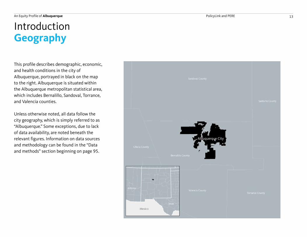
An Equity Profile of Albuquerque PolicyLink and PERE 13
Geography
This profile describes demographic, economic,
and health conditions in the city of
Albuquerque, portrayed in black on the map
to the right. Albuquerque is situated within
the Albuquerque metropolitan statistical area,
which includes Bernalillo, Sandoval, Torrance,
and Valencia counties.
Unless otherwise noted, all data follow the
city geography, which is simply referred to as
“Albuquerque.” Some exceptions, due to lack
of data availability, are noted beneath the
relevant figures. Information on data sources
and methodology can be found in the “Data
and methods” section beginning on page 95.
Introduction
An Equity Profile of Albuquerque PolicyLink and PERE 14
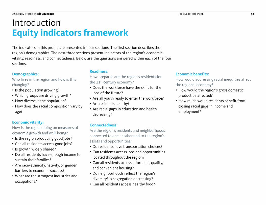
Equity indicators framework
Demographics:
Who lives in the region and how is this
changing?
• Is the population growing?
• Which groups are driving growth?
• How diverse is the population?
• How does the racial composition vary by
age?
Economic vitality:
How is the region doing on measures of
economic growth and well-being?
• Is the region producing good jobs?
• Can all residents access good jobs?
• Is growth widely shared?
• Do all residents have enough income to
sustain their families?
• Are race/ethnicity, nativity, or gender
barriers to economic success?
• What are the strongest industries and
occupations?
Introduction
Readiness:
How prepared are the region’s residents for
the 21st century economy?
• Does the workforce have the skills for the
jobs of the future?
• Are all youth ready to enter the workforce?
• Are residents healthy?
• Are racial gaps in education and health
decreasing?
Connectedness:
Are the region’s residents and neighborhoods
connected to one another and to the region’s
assets and opportunities?
• Do residents have transportation choices?
• Can residents access jobs and opportunities
located throughout the region?
• Can all residents access affordable, quality,
and convenient housing?
• Do neighborhoods reflect the region’s
diversity? Is segregation decreasing?
• Can all residents access healthy food?
The indicators in this profile are presented in four sections. The first section describes the
region’s demographics. The next three sections present indicators of the region’s economic
vitality, readiness, and connectedness. Below are the questions answered within each of the four
sections.
Economic benefits:
How would addressing racial inequities affect
the regional economy?
• How would the region’s gross domestic
product be affected?
• How much would residents benefit from
closing racial gaps in income and
employment?
An Equity Profile of Albuquerque PolicyLink and PERE 15
Demographics
An Equity Profile of Albuquerque PolicyLink and PERE 16
Highlights
Share of population that are Latino residents:
Demographics
Increase in people of color population since 1980:
Racial generation gap:
47%
143%
38
Who lives in the city and how is it changing?
• By 2014, more than half of Albuquerque
residents (59 percent) were people of color
– up from 40 percent of residents in 1980.
• Of the more than 324,700 people of color in
Albuquerque, 81 percent are Latino.
• There is a growing racial generation gap in
the region: 74 percent of youth are people
of color while only 37 percent of seniors are.
• Diverse groups, especially Latinos, Asian or
Pacific Islanders, Native Americans, and
those of mixed or other racial backgrounds
are driving growth.
percentage points
An Equity Profile of Albuquerque PolicyLink and PERE 17
40%
2%3%
0.2%
40%
7%
1%2%
4% 2%
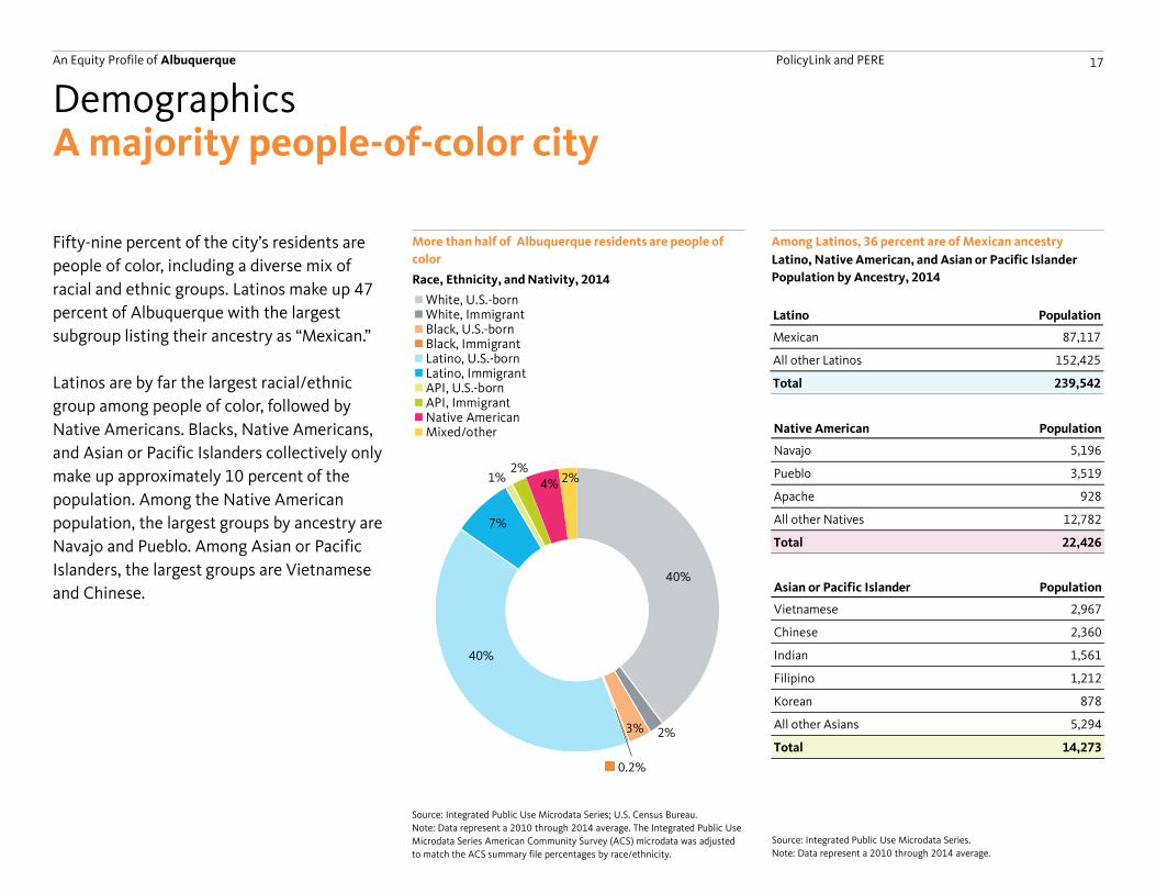
A majority people-of-color city
Fifty-nine percent of the city’s residents are
people of color, including a diverse mix of
racial and ethnic groups. Latinos make up 47
percent of Albuquerque with the largest
subgroup listing their ancestry as “Mexican.”
Latinos are by far the largest racial/ethnic
group among people of color, followed by
Native Americans. Blacks, Native Americans,
and Asian or Pacific Islanders collectively only
make up approximately 10 percent of the
population. Among the Native American
population, the largest groups by ancestry are
Navajo and Pueblo. Among Asian or Pacific
Islanders, the largest groups are Vietnamese
and Chinese.
More than half of Albuquerque residents are people of
color
Demographics
Race, Ethnicity, and Nativity, 2014
Source: Integrated Public Use Microdata Series.
Note: Data represent a 2010 through 2014 average.
Source: Integrated Public Use Microdata Series; U.S. Census Bureau.
Note: Data represent a 2010 through 2014 average. The Integrated Public Use
Microdata Series American Community Survey (ACS) microdata was adjusted
to match the ACS summary file percentages by race/ethnicity.
Among Latinos, 36 percent are of Mexican ancestry
Latino, Native American, and Asian or Pacific Islander
Population by Ancestry, 2014
Latino Population
Mexican 87,117
All other Latinos 152,425
Total 239,542
Native American Population
Navajo 5,196
Pueblo 3,519
Apache 928
All other Natives 12,782
Total 22,426
Asian or Pacific Islander Population
Vietnamese 2,967
Chinese 2,360
Indian 1,561
Filipino 1,212
Korean 878
All other Asians 5,294
Total 14,273
40%
2%3%
0.2%40%
7%
1%
2%
4%
2%
White, U.S.-bornWhite, ImmigrantBlack, U.S.-bornBlack, ImmigrantLatino, U.S.-bornLatino, ImmigrantAPI, U.S.-bornAPI, ImmigrantNative AmericanMixed/other
An Equity Profile of Albuquerque PolicyLink and PERE 18
Decline of 17% or more
Decline of less than 17% or no growth
Increase of less than 38%
Increase of 38% to 99%
Increase of 99% or more
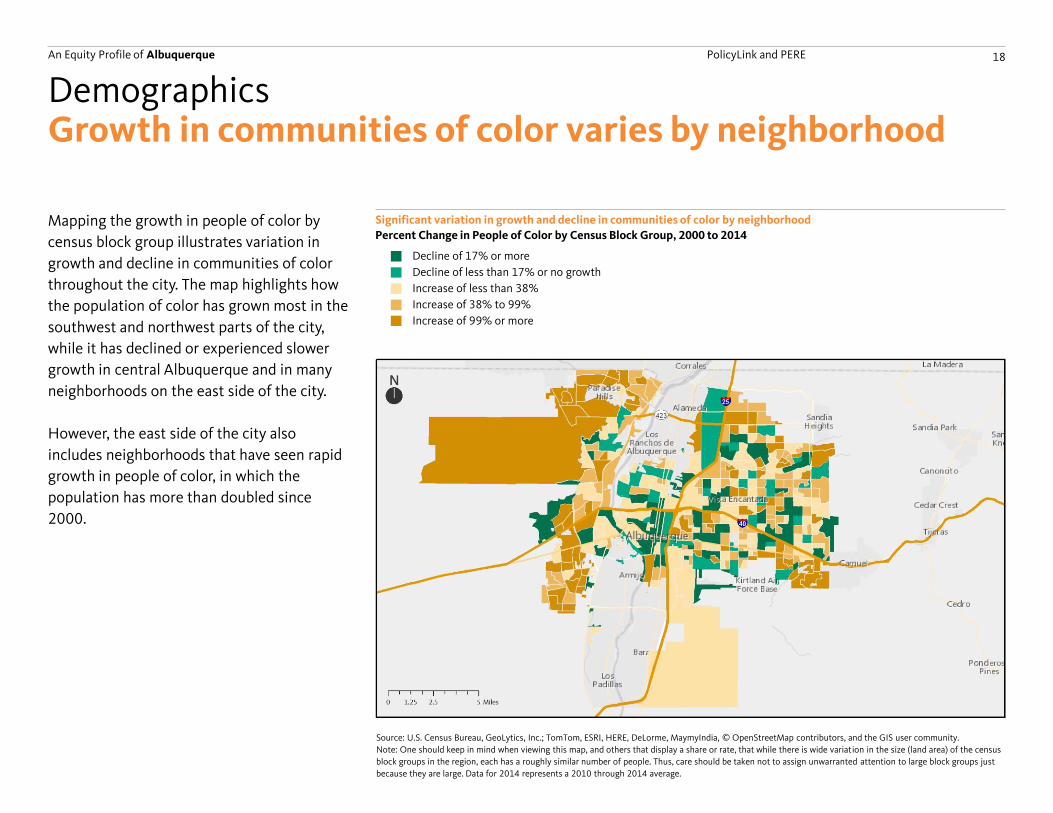
Growth in communities of color varies by neighborhood
Mapping the growth in people of color by
census block group illustrates variation in
growth and decline in communities of color
throughout the city. The map highlights how
the population of color has grown most in the
southwest and northwest parts of the city,
while it has declined or experienced slower
growth in central Albuquerque and in many
neighborhoods on the east side of the city.
However, the east side of the city also
includes neighborhoods that have seen rapid
growth in people of color, in which the
population has more than doubled since
2000.
Significant variation in growth and decline in communities of color by neighborhood
Demographics
Percent Change in People of Color by Census Block Group, 2000 to 2014
Source: U.S. Census Bureau, GeoLytics, Inc.; TomTom, ESRI, HERE, DeLorme, MaymyIndia, © OpenStreetMap contributors, and the GIS user community.
Note: One should keep in mind when viewing this map, and others that display a share or rate, that while there is wide variation in the size (land area) of the census
block groups in the region, each has a roughly similar number of people. Thus, care should be taken not to assign unwarranted attention to large block groups just
because they are large. Data for 2014 represents a 2010 through 2014 average.
An Equity Profile of Albuquerque PolicyLink and PERE 19
60% 59%
50%41%
2% 3%
3%
3%
34%34%
40%47%
2%2% 3%
2% 3%3% 4%2% 2%
1980 1990 2000 2014
25,112
-4,569
25,59028,274
62,927
79,379
1980 to 1990 1990 to 2000 2000 to 2014
WhitePeople of Color
25,112
-4,569 -1,052
28,274
62,927
99,983
1980 to 1990 1990 to 2000 2000 to 2014
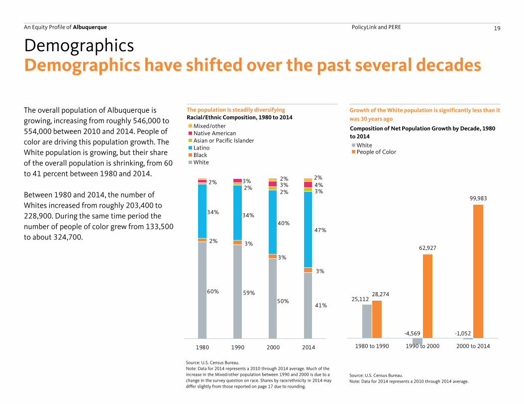
Demographics have shifted over the past several decades
The overall population of Albuquerque is
growing, increasing from roughly 546,000 to
554,000 between 2010 and 2014. People of
color are driving this population growth. The
White population is growing, but their share
of the overall population is shrinking, from 60
to 41 percent between 1980 and 2014.
Between 1980 and 2014, the number of
Whites increased from roughly 203,400 to
228,900. During the same time period the
number of people of color grew from 133,500
to about 324,700.
The population is steadily diversifying
Demographics
Racial/Ethnic Composition, 1980 to 2014
Source: U.S. Census Bureau.
Note: Data for 2014 represents a 2010 through 2014 average.
Source: U.S. Census Bureau.
Note: Data for 2014 represents a 2010 through 2014 average. Much of the
increase in the Mixed/other population between 1990 and 2000 is due to a
change in the survey question on race. Shares by race/ethnicity in 2014 may
differ slightly from those reported on page 17 due to rounding.
Growth of the White population is significantly less than it
was 30 years ago
Composition of Net Population Growth by Decade, 1980
to 2014
60% 59%50%
45%
2% 3%
3%
3%
34% 34%
40%43%
1% 2%2% 3%
2%
1980 1990 2000 2014
Mixed/otherNative AmericanAsian or Pacific IslanderLatinoBlackWhite
An Equity Profile of Albuquerque PolicyLink and PERE 20
17%
83%
2%
29%
46%
41%
40%
40%
White
Black
Latino
Asian orPacific Islander
Native American
Mixed/other19%
81%
19%
81%
Foreign-born Black
U.S.-born Black
All major subgroups are experiencing growth since 2000
Latinos grew the most since 2000, followed by Asian or
Pacific Islanders, Native Americans, and Mixed/other
Demographics
Growth Rates of Major Racial/Ethnic Groups,
2000 to 2014
Source: Integrated Public Use Microdata Series.
Note: Data for 2014 represents a 2010 through 2014 average.
Source: U.S. Census Bureau.
Note: Data for 2014 represents a 2010 through 2014 average.
Both Black and Latino population growth are largely
driven by U.S. born populations
Share of Net Growth in Black and Latino Population by
Nativity, 2000 to 2014
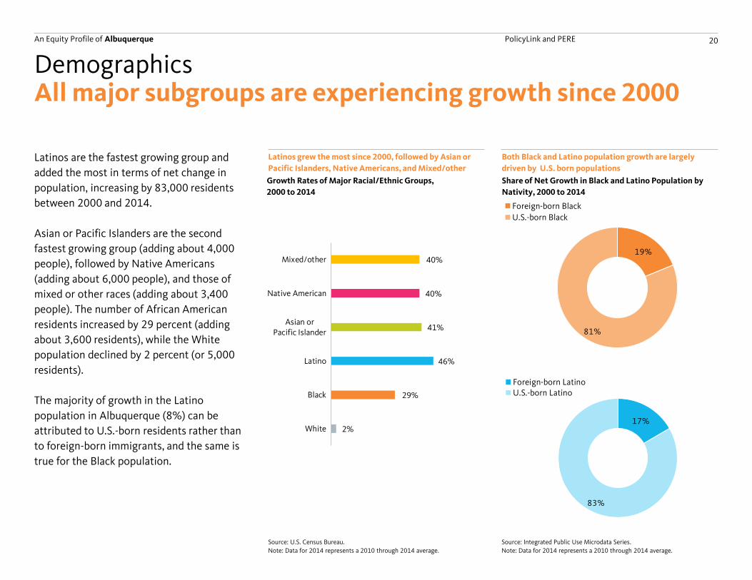
Latinos are the fastest growing group and
added the most in terms of net change in
population, increasing by 83,000 residents
between 2000 and 2014.
Asian or Pacific Islanders are the second
fastest growing group (adding about 4,000
people), followed by Native Americans
(adding about 6,000 people), and those of
mixed or other races (adding about 3,400
people). The number of African American
residents increased by 29 percent (adding
about 3,600 residents), while the White
population declined by 2 percent (or 5,000
residents).
The majority of growth in the Latino
population in Albuquerque (8%) can be
attributed to U.S.-born residents rather than
to foreign-born immigrants, and the same is
true for the Black population.
17%
83%
Foreign-born LatinoU.S.-born Latino
An Equity Profile of Albuquerque PolicyLink and PERE 21
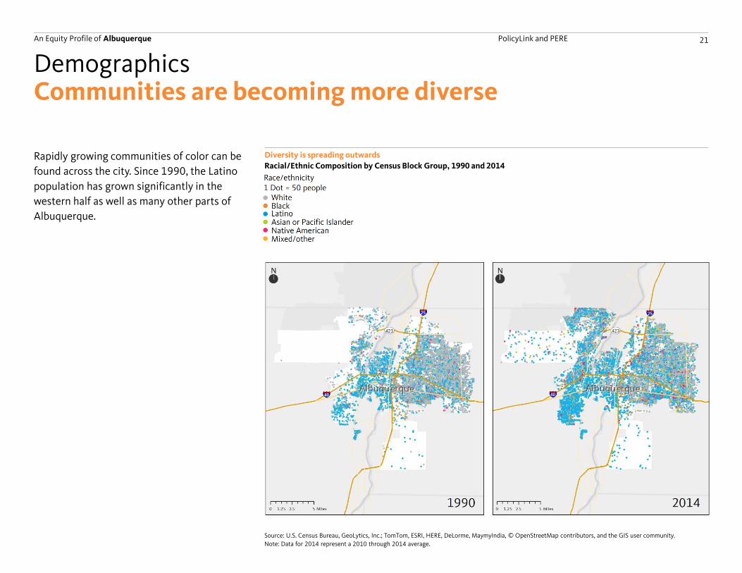
Communities are becoming more diverse
Rapidly growing communities of color can be
found across the city. Since 1990, the Latino
population has grown significantly in the
western half as well as many other parts of
Albuquerque.
Diversity is spreading outwards
Demographics
Racial/Ethnic Composition by Census Block Group, 1990 and 2014
Source: U.S. Census Bureau, GeoLytics, Inc.; TomTom, ESRI, HERE, DeLorme, MaymyIndia, © OpenStreetMap contributors, and the GIS user community.
Note: Data for 2014 represent a 2010 through 2014 average.
An Equity Profile of Albuquerque PolicyLink and PERE 22
57%56%
48%41%
37%33%
28%25%
2% 2%
2%
2%3%
3%3%
3%
37% 37%42%
48%52%
55%58%
61%
2% 2% 3% 3% 3% 4%
2% 3% 4% 4% 4% 4% 4% 4%2% 2% 3% 3% 3%
1980 1990 2000 2010 2020 2030 2040 2050
Projected
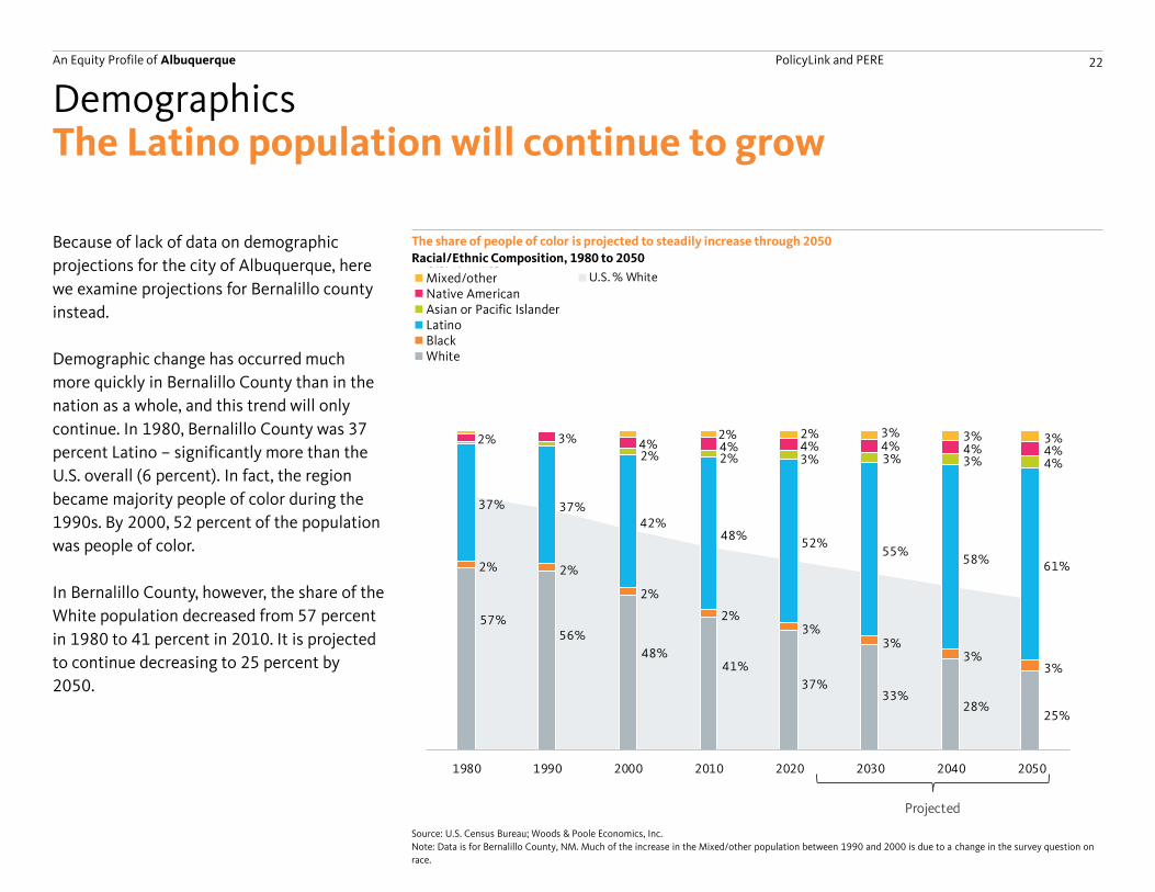
The Latino population will continue to grow
Because of lack of data on demographic
projections for the city of Albuquerque, here
we examine projections for Bernalillo county
instead.
Demographic change has occurred much
more quickly in Bernalillo County than in the
nation as a whole, and this trend will only
continue. In 1980, Bernalillo County was 37
percent Latino – significantly more than the
U.S. overall (6 percent). In fact, the region
became majority people of color during the
1990s. By 2000, 52 percent of the population
was people of color.
In Bernalillo County, however, the share of the
White population decreased from 57 percent
in 1980 to 41 percent in 2010. It is projected
to continue decreasing to 25 percent by
2050.
The share of people of color is projected to steadily increase through 2050
Demographics
Racial/Ethnic Composition, 1980 to 2050
Source: U.S. Census Bureau; Woods & Poole Economics, Inc.
Note: Data is for Bernalillo County, NM. Much of the increase in the Mixed/other population between 1990 and 2000 is due to a change in the survey question on
race.
65%
58%
48%
40%
34%
28%24%
18%
17%
17%
17%
16%
15%
14%
14% 21%29% 35% 41% 47% 52%
2% 3%5% 6% 7% 8% 9%
1% 1% 2% 2% 2%
1980 1990 2000 2010 2020 2030 2040
U.S. % White
Other
Native American
Asian/Pacific Islander
Latino
Black
White
Projected
90% 88%80% 76% 71%
65%59%
52%
7% 8%
9%9%
10%11%
12%13%
2% 3%7% 10%
12%16%
20%25%
1% 2% 2% 3% 3% 4% 4%
2% 3%
4%
5% 6%
1980 1990 2000 2010 2020 2030 2040 2050
U.S. % WhiteMixed/otherNative AmericanAsian or Pacific IslanderLatinoBlackWhite
Projected
An Equity Profile of Albuquerque PolicyLink and PERE 23
24%
37%
50%
74%
1980 1990 2000 2014
38 percentage point gap
26 percentage point gap
25
37
30
34
47
37
Mixed/other
Asian or Pacific Islander
Latino
Black
White
All
A growing racial generation gap
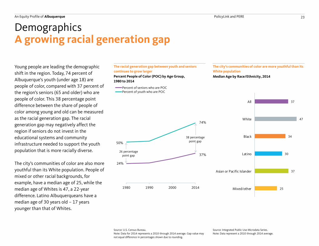
Young people are leading the demographic
shift in the region. Today, 74 percent of
Albuquerque’s youth (under age 18) are
people of color, compared with 37 percent of
the region’s seniors (65 and older) who are
people of color. This 38 percentage point
difference between the share of people of
color among young and old can be measured
as the racial generation gap. The racial
generation gap may negatively affect the
region if seniors do not invest in the
educational systems and community
infrastructure needed to support the youth
population that is more racially diverse.
The city’s communities of color are also more
youthful than its White population. People of
mixed or other racial backgrounds, for
example, have a median age of 25, while the
median age of Whites is 47, a 22-year
difference. Latino Albuquerqueans have a
median age of 30 years old – 17 years
younger than that of Whites.
The racial generation gap between youth and seniors
continues to grow larger
Demographics
Percent People of Color (POC) by Age Group,
1980 to 2014
Source: Integrated Public Use Microdata Series.
Note: Data represent a 2010 through 2014 average.
Source: U.S. Census Bureau.
Note: Data for 2014 represents a 2010 through 2014 average. Gap value may
not equal difference in percentages shown due to rounding.
The city’s communities of color are more youthful than its
White population
Median Age by Race/Ethnicity, 2014
24%
37%
50%
74%
1980 1990 2000 2014
Percent of seniors who are POCPercent of youth who are POC
21 percentage point gap
9 percentage point gap
An Equity Profile of Albuquerque PolicyLink and PERE 24
Irving City, TX: #1 (54)
Albuquerque: #18 (38)
Hialeah City, FL: #100 (-02)
A growing racial generation gap
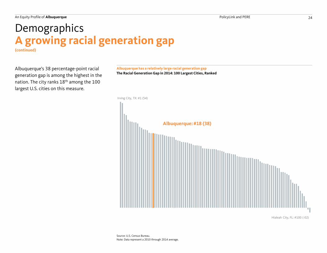
Albuquerque’s 38 percentage-point racial
generation gap is among the highest in the
nation. The city ranks 18th among the 100
largest U.S. cities on this measure.
Albuquerque has a relatively large racial generation gap
Demographics
The Racial Generation Gap in 2014: 100 Largest Cities, Ranked
(continued)
Source: U.S. Census Bureau.
Note: Data represent a 2010 through 2014 average.
An Equity Profile of Albuquerque PolicyLink and PERE 25
Economic vitality
An Equity Profile of Albuquerque PolicyLink and PERE 26
Wage growth for workers at the 10th percentile since 1979:
-11%
HighlightsEconomic vitality
Wage gap between college-educated people of color and Whites:
$4/hour
Share of Native Americans living in poverty:
32%
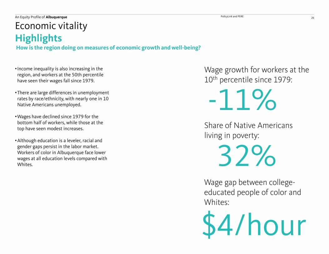
How is the region doing on measures of economic growth and well-being?
• Income inequality is also increasing in the region, and workers at the 50th percentile have seen their wages fall since 1979.
•There are large differences in unemployment rates by race/ethnicity, with nearly one in 10 Native Americans unemployed.
•Wages have declined since 1979 for the bottom half of workers, while those at the top have seen modest increases.
•Although education is a leveler, racial and gender gaps persist in the labor market. Workers of color in Albuquerque face lower wages at all education levels compared with Whites.
An Equity Profile of Albuquerque PolicyLink and PERE 27
89%
64%
-10%
30%
70%
110%
1979 1984 1989 1994 1999 2004 2009 2014
105%
106%
-10%
30%
70%
110%
1979 1984 1989 1994 1999 2004 2009 2014
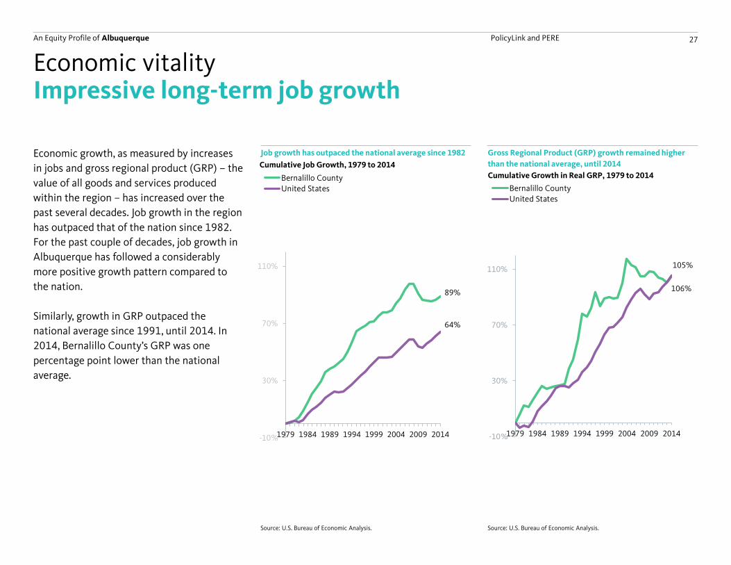
Impressive long-term job growth
Economic growth, as measured by increases
in jobs and gross regional product (GRP) – the
value of all goods and services produced
within the region – has increased over the
past several decades. Job growth in the region
has outpaced that of the nation since 1982.
For the past couple of decades, job growth in
Albuquerque has followed a considerably
more positive growth pattern compared to
the nation.
Similarly, growth in GRP outpaced the
national average since 1991, until 2014. In
2014, Bernalillo County’s GRP was one
percentage point lower than the national
average.
Job growth has outpaced the national average since 1982
Economic vitality
Cumulative Job Growth, 1979 to 2014
Source: U.S. Bureau of Economic Analysis.Source: U.S. Bureau of Economic Analysis.
Gross Regional Product (GRP) growth remained higher
than the national average, until 2014
Cumulative Growth in Real GRP, 1979 to 2014
89%
64%
0%
40%
80%
120%
1979 1984 1989 1994 1999 2004 2009 2014
Bernalillo CountyUnited States
89%
64%
0%
40%
80%
120%
1979 1984 1989 1994 1999 2004 2009 2014
Bernalillo CountyUnited States
An Equity Profile of Albuquerque PolicyLink and PERE 28
5.9%
5.3%
0
0.1
0.2
0.3
0.4
0.5
0.6
0.7
0.8
0.9
1
0%
4%
8%
12%
1990 1995 2000 2005 2010 2015
Downturn 2007-2010
A slow recovery post-recession
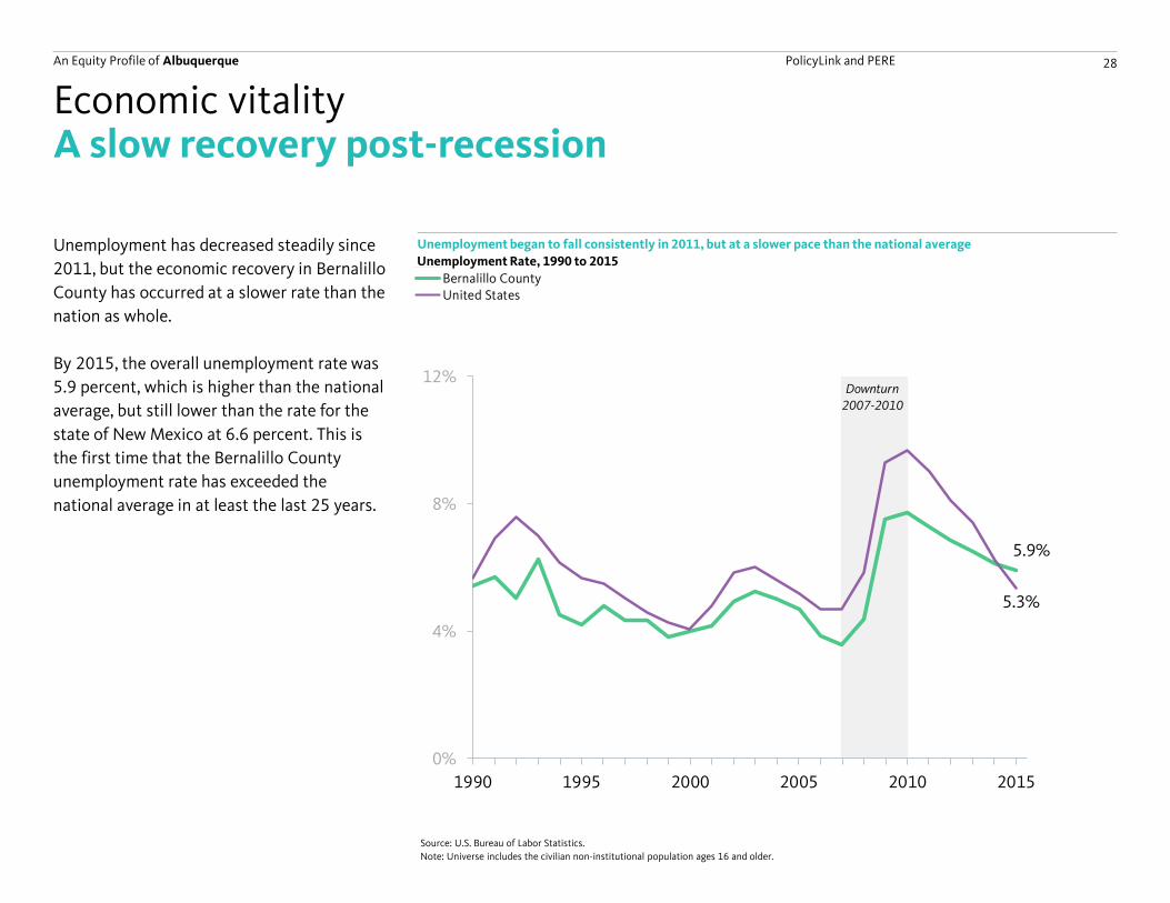
Unemployment has decreased steadily since
2011, but the economic recovery in Bernalillo
County has occurred at a slower rate than the
nation as whole.
By 2015, the overall unemployment rate was
5.9 percent, which is higher than the national
average, but still lower than the rate for the
state of New Mexico at 6.6 percent. This is
the first time that the Bernalillo County
unemployment rate has exceeded the
national average in at least the last 25 years.
Unemployment began to fall consistently in 2011, but at a slower pace than the national average
Economic vitality
Unemployment Rate, 1990 to 2015
Source: U.S. Bureau of Labor Statistics.
Note: Universe includes the civilian non-institutional population ages 16 and older.
0
0.1
0.2
0.3
0.4
0.5
0.6
0.7
0.8
0.9
1
0%
4%
8%
12%
1990 1992 1994 1996 1998 2000 2002 2004 2006 2008 2010 2012 2014
Bernalillo CountyUnited States
Downturn 2007-2010

An Equity Profile of Albuquerque PolicyLink and PERE 29
15%16%
-10%
0%
10%
20%
30%
40%
1979 1984 1989 1994 1999 2004 2009 2014
Job growth is keeping up with population growth
While overall job growth is essential, it’s
important to consider whether jobs are
growing at a fast enough pace to keep up with
population growth. Bernalillo County’s job
growth per person has been higher than the
national average since 1982. The number of
jobs per person in Bernalillo County has
increased notably since it’s nadir in 1981, but
the rate in 2014 was less than half of what it
was at its peak in 2001.
While an increase in the jobs to population
ratio is good, it does not explain whether
workers with barriers to employment have
access to those jobs.
Job growth relative to population growth was higher than the national average until 2012
Economic vitality
Cumulative Growth in Jobs-to-Population Ratio, 1979 to 2014
Source: U.S. Bureau of Economic Analysis.
0
0.1
0.2
0.3
0.4
0.5
0.6
0.7
0.8
0.9
1
0%
4%
8%
12%
1990 1992 1994 1996 1998 2000 2002 2004 2006 2008 2010 2012 2014
Bernalillo CountyUnited States
Downturn 2007-2010
An Equity Profile of Albuquerque PolicyLink and PERE 30
7.8%
9.4%
7.3%
7.7%
5.8%
5.9%
10.0%
7.7%
6.5%
7.0%
3.3%
Mixed/other
Native American
Asian orPacific Islander
Latino
Black
White
76%
77%
78%
77%
74%
78%
81%
77%
76%
84%
80%
Mixed/other
Native American
Asian orPacific Islander
Latino
Black
White
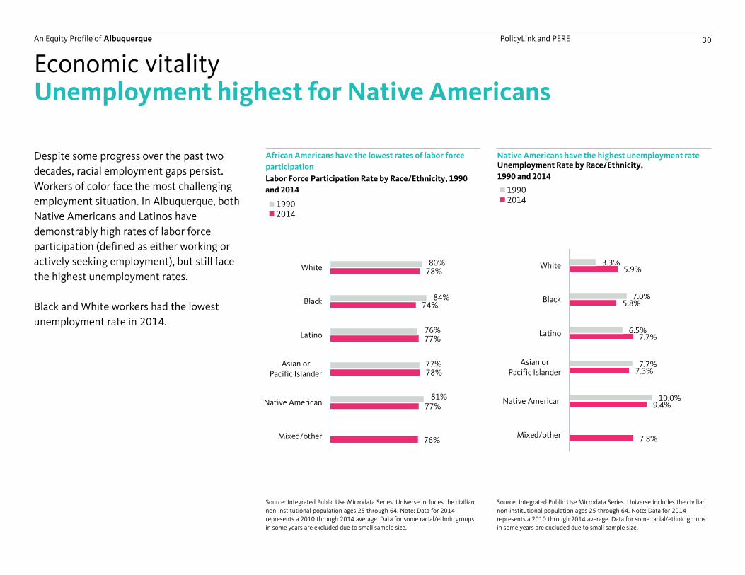
Unemployment highest for Native Americans
Despite some progress over the past two
decades, racial employment gaps persist.
Workers of color face the most challenging
employment situation. In Albuquerque, both
Native Americans and Latinos have
demonstrably high rates of labor force
participation (defined as either working or
actively seeking employment), but still face
the highest unemployment rates.
Black and White workers had the lowest
unemployment rate in 2014.
African Americans have the lowest rates of labor force
participation
Economic vitality
Labor Force Participation Rate by Race/Ethnicity, 1990
and 2014
Source: Integrated Public Use Microdata Series. Universe includes the civilian
non-institutional population ages 25 through 64. Note: Data for 2014
represents a 2010 through 2014 average. Data for some racial/ethnic groups
in some years are excluded due to small sample size.
Source: Integrated Public Use Microdata Series. Universe includes the civilian
non-institutional population ages 25 through 64. Note: Data for 2014
represents a 2010 through 2014 average. Data for some racial/ethnic groups
in some years are excluded due to small sample size.
Native Americans have the highest unemployment rateUnemployment Rate by Race/Ethnicity,
1990 and 2014
78%
77%
74%
78%
77%
76%
84%
80%
Native American
Asian orPacific Islander
Latino
Black
19902014
78%
77%
74%
78%
77%
76%
84%
80%
Native American
Asian orPacific Islander
Latino
Black
19902014
An Equity Profile of Albuquerque PolicyLink and PERE 31
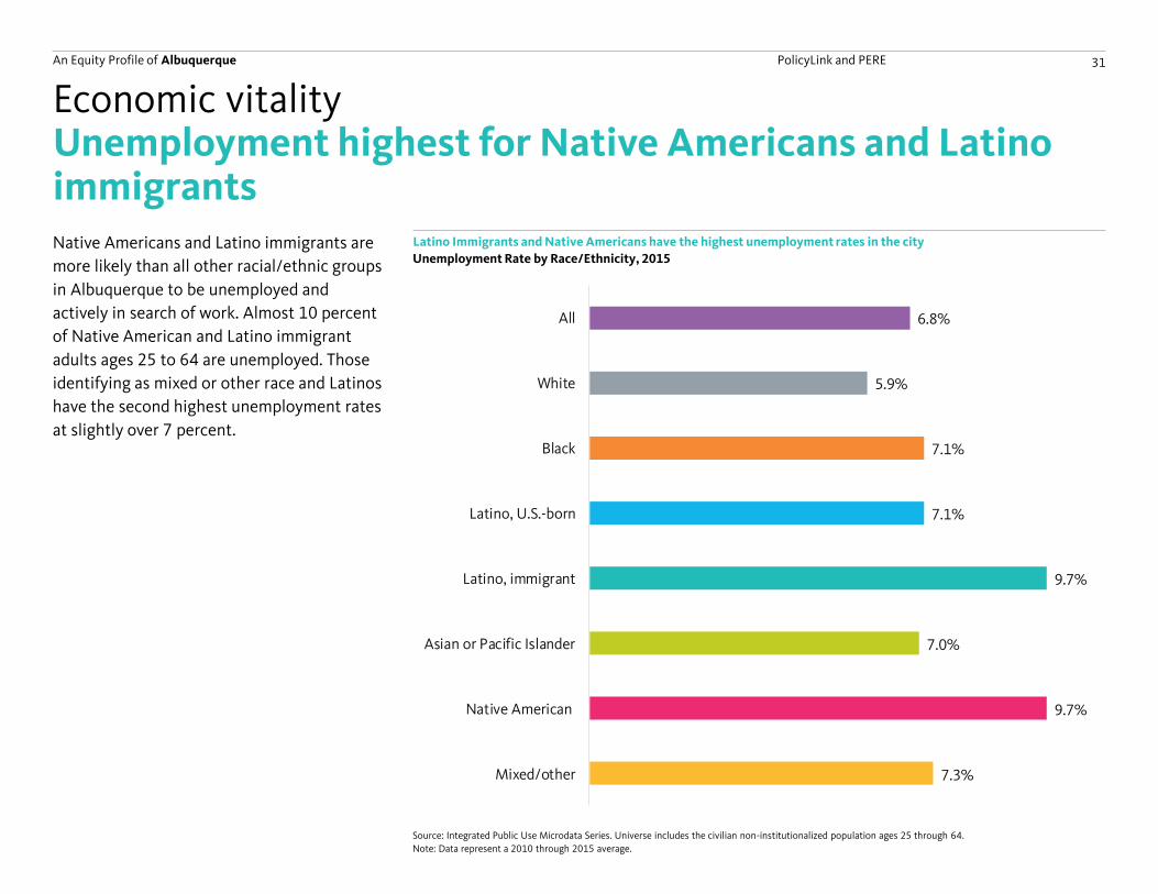
Unemployment highest for Native Americans and Latino immigrantsNative Americans and Latino immigrants are
more likely than all other racial/ethnic groups
in Albuquerque to be unemployed and
actively in search of work. Almost 10 percent
of Native American and Latino immigrant
adults ages 25 to 64 are unemployed. Those
identifying as mixed or other race and Latinos
have the second highest unemployment rates
at slightly over 7 percent.
Latino Immigrants and Native Americans have the highest unemployment rates in the city
Economic vitality
Unemployment Rate by Race/Ethnicity, 2015
Source: Integrated Public Use Microdata Series. Universe includes the civilian non-institutionalized population ages 25 through 64.
Note: Data represent a 2010 through 2015 average.
6.8%
5.9%
7.1%
7.1%
9.7%
7.0%
9.7%
7.3%
All
White
Black
Latino, U.S.-born
Latino, immigrant
Asian or Pacific Islander
Native American
Mixed/other
An Equity Profile of Albuquerque PolicyLink and PERE 32
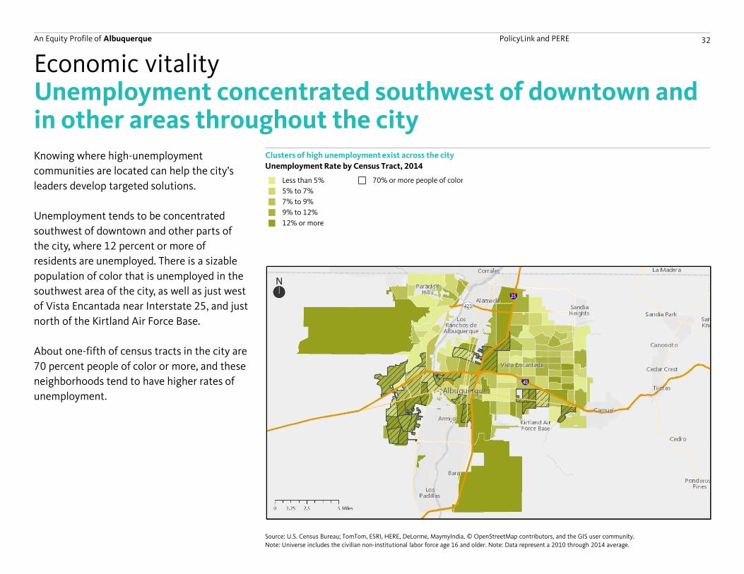
Unemployment concentrated southwest of downtown and in other areas throughout the cityKnowing where high-unemployment
communities are located can help the city’s
leaders develop targeted solutions.
Unemployment tends to be concentrated
southwest of downtown and other parts of
the city, where 12 percent or more of
residents are unemployed. There is a sizable
population of color that is unemployed in the
southwest area of the city, as well as just west
of Vista Encantada near Interstate 25, and just
north of the Kirtland Air Force Base.
About one-fifth of census tracts in the city are
70 percent people of color or more, and these
neighborhoods tend to have higher rates of
unemployment.
Clusters of high unemployment exist across the city
Economic vitality
Unemployment Rate by Census Tract, 2014
Less than 5%
5% to 7%
7% to 9%
9% to 12%
12% or more
70% or more people of color
Source: U.S. Census Bureau; TomTom, ESRI, HERE, DeLorme, MaymyIndia, © OpenStreetMap contributors, and the GIS user community.
Note: Universe includes the civilian non-institutional labor force age 16 and older. Note: Data represent a 2010 through 2014 average.
An Equity Profile of Albuquerque PolicyLink and PERE 33
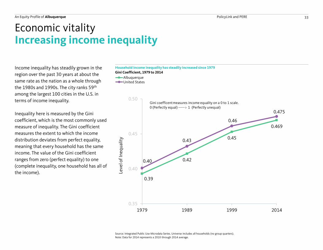
0.40
0.43
0.46
0.475
0.39
0.42
0.45
0.469
0.35
0.40
0.45
0.50
1979 1989 1999 2014
Leve
l of
Ineq
ual
ity
Gini coefficent measures income equality on a 0 to 1 scale.0 (Perfectly equal) ------> 1 (Perfectly unequal)
Increasing income inequality
Income inequality has steadily grown in the
region over the past 30 years at about the
same rate as the nation as a whole through
the 1980s and 1990s. The city ranks 59th
among the largest 100 cities in the U.S. in
terms of income inequality.
Inequality here is measured by the Gini
coefficient, which is the most commonly used
measure of inequality. The Gini coefficient
measures the extent to which the income
distribution deviates from perfect equality,
meaning that every household has the same
income. The value of the Gini coefficient
ranges from zero (perfect equality) to one
(complete inequality, one household has all of
the income).
Household income inequality has steadily increased since 1979
Economic vitality
Gini Coefficient, 1979 to 2014
Source: Integrated Public Use Microdata Series. Universe includes all households (no group quarters).
Note: Data for 2014 represents a 2010 through 2014 average.
0.39
0.42
0.45
0.47
0.40
0.43
0.46
0.47
0.35
0.40
0.45
0.50
0.55
1979 1989 1999 2014
Leve
l o
f In
equ
alit
y
AlbuquerqueUnited States
Gini Coefficent measures income equality on a 0 to 1 scale.0 (Perfectly equal) ------> 1 (Perfectly unequal)
An Equity Profile of Albuquerque PolicyLink and PERE 34
-11.4% -10.3%
-2%
4% 5%
-11% -10%-7%
6%
17%
10th Percentile 20th Percentile 50th Percentile 80th Percentile 90th Percentile
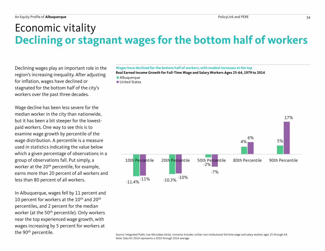
Declining or stagnant wages for the bottom half of workers
Declining wages play an important role in the
region’s increasing inequality. After adjusting
for inflation, wages have declined or
stagnated for the bottom half of the city’s
workers over the past three decades.
Wage decline has been less severe for the
median worker in the city than nationwide,
but it has been a bit steeper for the lowest-
paid workers. One way to see this is to
examine wage growth by percentile of the
wage distribution. A percentile is a measure
used in statistics indicating the value below
which a given percentage of observations in a
group of observations fall. Put simply, a
worker at the 20th percentile, for example,
earns more than 20 percent of all workers and
less than 80 percent of all workers.
In Albuquerque, wages fell by 11 percent and
10 percent for workers at the 10th and 20th
percentiles, and 2 percent for the median
worker (at the 50th percentile). Only workers
near the top experienced wage growth, with
wages increasing by 5 percent for workers at
the 90th percentile.
Wages have declined for the bottom half of workers, with modest increases at the top
Economic vitality
Real Earned Income Growth for Full-Time Wage and Salary Workers Ages 25-64, 1979 to 2014
Source: Integrated Public Use Microdata Series. Universe includes civilian non-institutional full-time wage and salary workers ages 25 through 64.
Note: Data for 2014 represents a 2010 through 2014 average.
-11%-10%
-2%
4% 5%
-11.0%-9.9%
-7%
6%
17%
10th Percentile 20th Percentile 50th Percentile 80th Percentile 90th Percentile
AlbuquerqueUnited States
An Equity Profile of Albuquerque PolicyLink and PERE 35
$20.20
$22.40
$17.80 $17.10
$20.50
$14.30
$20.50
$17.10
$20.40
$24.30
$19.90$17.50
$19.90
$14.80
$19.30$17.50
Modest wage growth
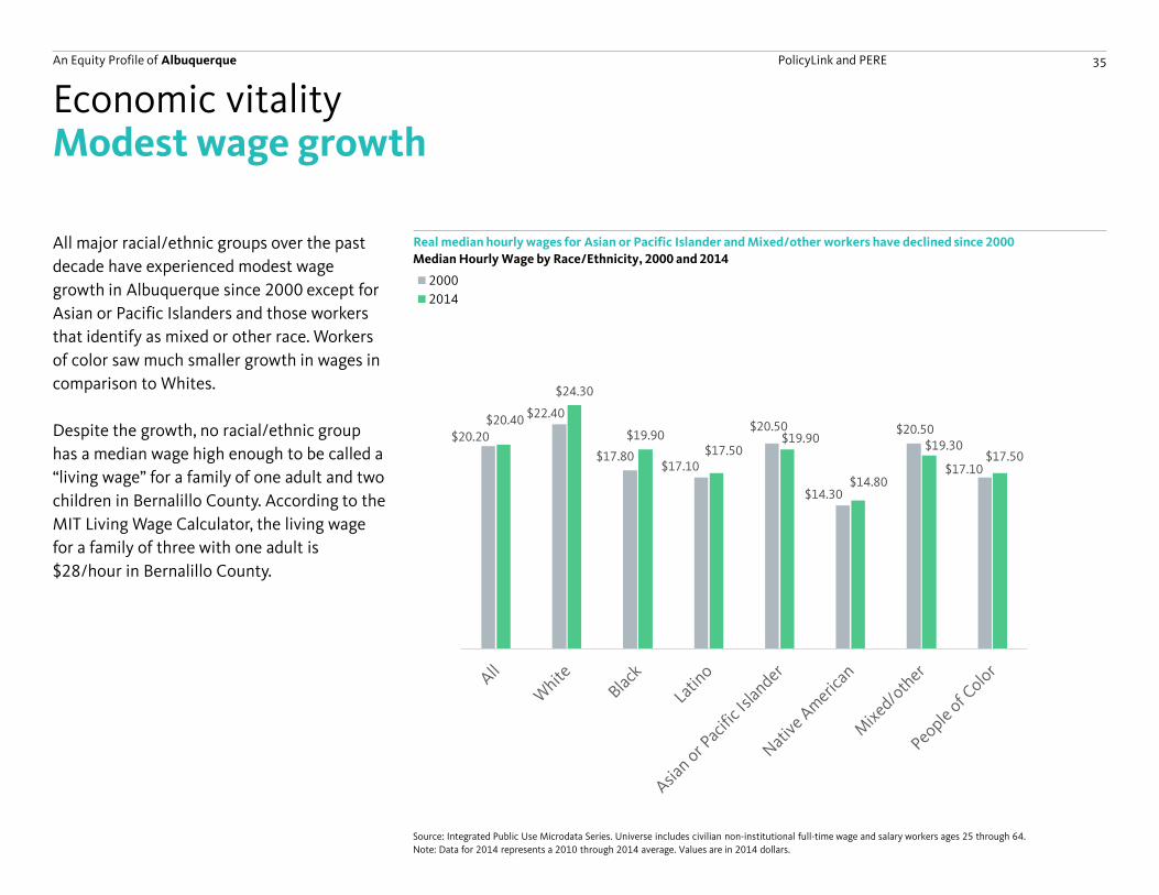
All major racial/ethnic groups over the past
decade have experienced modest wage
growth in Albuquerque since 2000 except for
Asian or Pacific Islanders and those workers
that identify as mixed or other race. Workers
of color saw much smaller growth in wages in
comparison to Whites.
Despite the growth, no racial/ethnic group
has a median wage high enough to be called a
“living wage” for a family of one adult and two
children in Bernalillo County. According to the
MIT Living Wage Calculator, the living wage
for a family of three with one adult is
$28/hour in Bernalillo County.
Real median hourly wages for Asian or Pacific Islander and Mixed/other workers have declined since 2000
Economic vitality
Median Hourly Wage by Race/Ethnicity, 2000 and 2014
Source: Integrated Public Use Microdata Series. Universe includes civilian non-institutional full-time wage and salary workers ages 25 through 64.
Note: Data for 2014 represents a 2010 through 2014 average. Values are in 2014 dollars.
$22.40
$17.80 $17.10
$20.50 $20.50
$24.30
$19.90
$17.50
$19.90 $19.30
White Black Latino Asian or PacificIslander
Mixed/other
2000
2014
An Equity Profile of Albuquerque PolicyLink and PERE 36
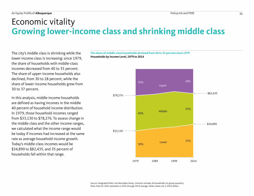
30%37%
40%
35%
30% 28%
1979 1989 1999 2014
Lower
Middle
Upper
$33,130
$78,276 $82,435
$34,890
Growing lower-income class and shrinking middle class
The city’s middle class is shrinking while the
lower-income class is increasing: since 1979,
the share of households with middle-class
incomes decreased from 40 to 35 percent.
The share of upper-income households also
declined, from 30 to 28 percent, while the
share of lower-income households grew from
30 to 37 percent.
In this analysis, middle-income households
are defined as having incomes in the middle
40 percent of household income distribution.
In 1979, those household incomes ranged
from $33,130 to $78,276. To assess change in
the middle class and the other income ranges,
we calculated what the income range would
be today if incomes had increased at the same
rate as average household income growth.
Today’s middle-class incomes would be
$34,890 to $82,435, and 35 percent of
households fall within that range.
The share of middle-class households declined from 40 to 35 percent since 1979
Economic vitality
Households by Income Level, 1979 to 2014
Source: Integrated Public Use Microdata Series. Universe includes all households (no group quarters).
Note: Data for 2014 represents a 2010 through 2014 average. Dollar values are in 2014 dollars.
An Equity Profile of Albuquerque PolicyLink and PERE 37
65% 67%
55% 54%
2% 2%
2% 3%
30% 28%35% 36%
3% 3% 7% 8%
Middle-ClassHouseholds
All Households Middle-ClassHouseholds
All Households
1979 2014
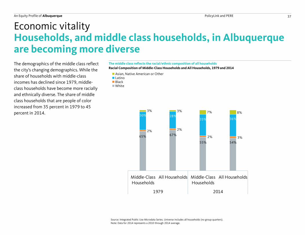
Households, and middle class households, in Albuquerque are becoming more diverse The demographics of the middle class reflect
the city’s changing demographics. While the
share of households with middle-class
incomes has declined since 1979, middle-
class households have become more racially
and ethnically diverse. The share of middle
class households that are people of color
increased from 35 percent in 1979 to 45
percent in 2014.
The middle class reflects the racial/ethnic composition of all households
Economic vitality
Racial Composition of Middle-Class Households and All Households, 1979 and 2014
Source: Integrated Public Use Microdata Series. Universe includes all households (no group quarters).
Note: Data for 2014 represents a 2010 through 2014 average.
65% 67%
55%54%
2%2%
2% 3%
30%28%
35% 36%
3% 3%7% 8%
Middle-ClassHouseholds
All Households Middle-ClassHouseholds
All Households
1979 2014
Asian, Native American or OtherLatinoBlackWhite
An Equity Profile of Albuquerque PolicyLink and PERE 38
18.6%
15.7%
0%
10%
20%
1980 1990 2000 2014
10.1%9.0%
0%
10%
20%
1980 1990 2000 2014
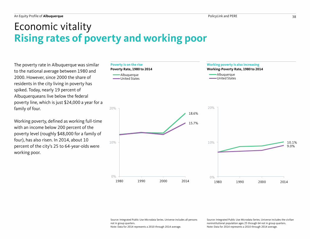
Rising rates of poverty and working poor
The poverty rate in Albuquerque was similar
to the national average between 1980 and
2000. However, since 2000 the share of
residents in the city living in poverty has
spiked. Today, nearly 19 percent of
Albuquerqueans live below the federal
poverty line, which is just $24,000 a year for a
family of four.
Working poverty, defined as working full-time
with an income below 200 percent of the
poverty level (roughly $48,000 for a family of
four), has also risen. In 2014, about 10
percent of the city’s 25 to 64-year-olds were
working poor.
Poverty is on the rise
Economic vitality
Poverty Rate, 1980 to 2014
Source: Integrated Public Use Microdata Series. Universe includes the civilian
noninstitutional population ages 25 through 64 not in group quarters.
Note: Data for 2014 represents a 2010 through 2014 average.
Source: Integrated Public Use Microdata Series. Universe includes all persons
not in group quarters.
Note: Data for 2014 represents a 2010 through 2014 average.
Working poverty is also increasing
Working-Poverty Rate, 1980 to 2014
18.6%
15.7%
0%
2%
4%
6%
8%
10%
12%
14%
16%
18%
20%
1980 1990 2000 2014
AlbuquerqueUnited States
18.6%
15.7%
0%
2%
4%
6%
8%
10%
12%
14%
16%
18%
20%
1980 1990 2000 2014
AlbuquerqueUnited States
An Equity Profile of Albuquerque PolicyLink and PERE 39
10%
6%
14.2%14.2%
12%
20%
13.8%
0%
5%
10%
15%
20%
25%
18.6%
12%
23%25%
13%
32%
19.2%
0%
10%
20%
30%
40%
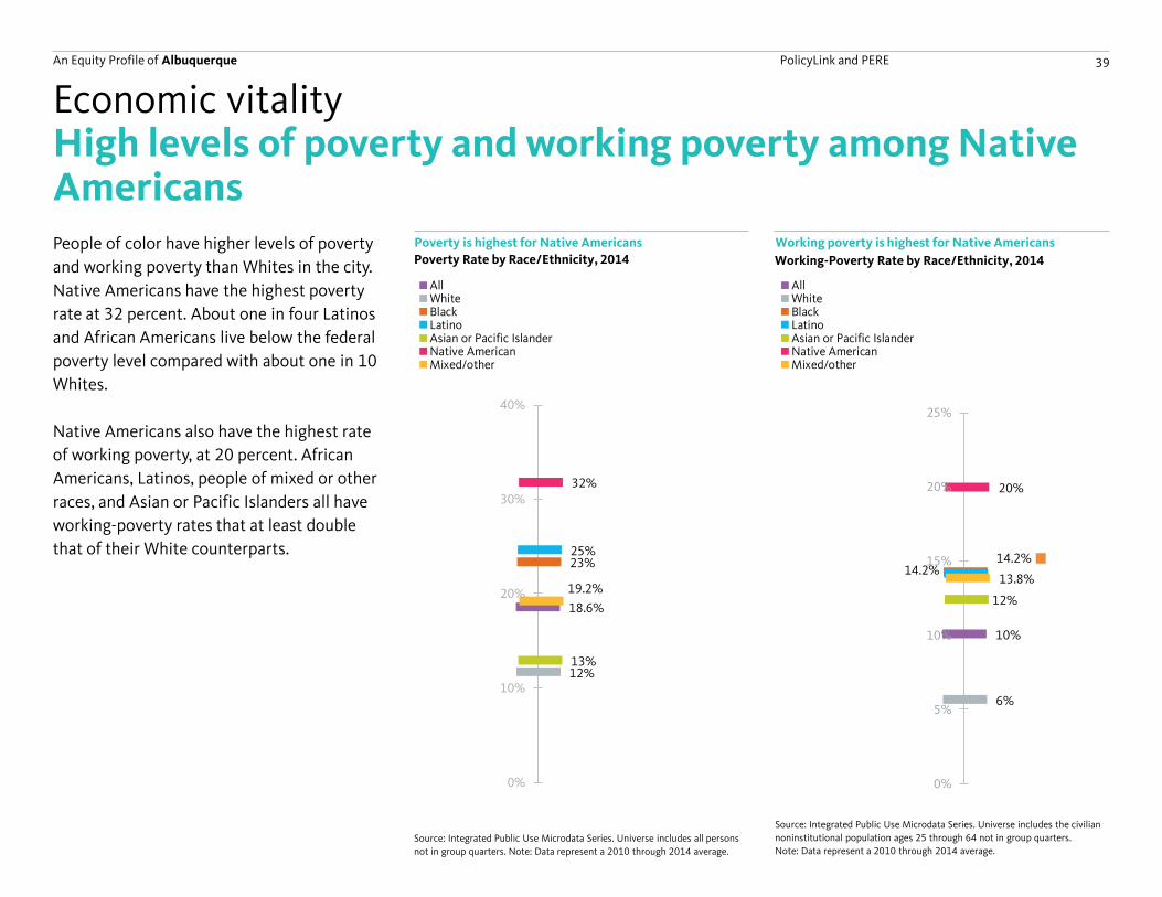
High levels of poverty and working poverty among Native AmericansPeople of color have higher levels of poverty
and working poverty than Whites in the city.
Native Americans have the highest poverty
rate at 32 percent. About one in four Latinos
and African Americans live below the federal
poverty level compared with about one in 10
Whites.
Native Americans also have the highest rate
of working poverty, at 20 percent. African
Americans, Latinos, people of mixed or other
races, and Asian or Pacific Islanders all have
working-poverty rates that at least double
that of their White counterparts.
Poverty is highest for Native Americans
Economic vitality
Poverty Rate by Race/Ethnicity, 2014
Source: Integrated Public Use Microdata Series. Universe includes the civilian
noninstitutional population ages 25 through 64 not in group quarters.
Note: Data represent a 2010 through 2014 average.Source: Integrated Public Use Microdata Series. Universe includes all persons
not in group quarters. Note: Data represent a 2010 through 2014 average.
Working poverty is highest for Native Americans
Working-Poverty Rate by Race/Ethnicity, 2014
18.6%
12%
23%25%
13%
32%
19.2%
0%
10%
20%
30%
40%
AllWhiteBlackLatinoAsian or Pacific IslanderNative AmericanMixed/other
18.6%
12%
23%25%
13%
32%
19.2%
0%
10%
20%
30%
40%
AllWhiteBlackLatinoAsian or Pacific IslanderNative AmericanMixed/other
An Equity Profile of Albuquerque PolicyLink and PERE 40
39%
15%
34%
17%
42%
24%
10%
28%
11%
26%25%
11%
35%
16%
37%
22%
26%
12%
34%
19%
29%
26%
Black White Latino Asian or PacificIslander
Native American Mixed/other
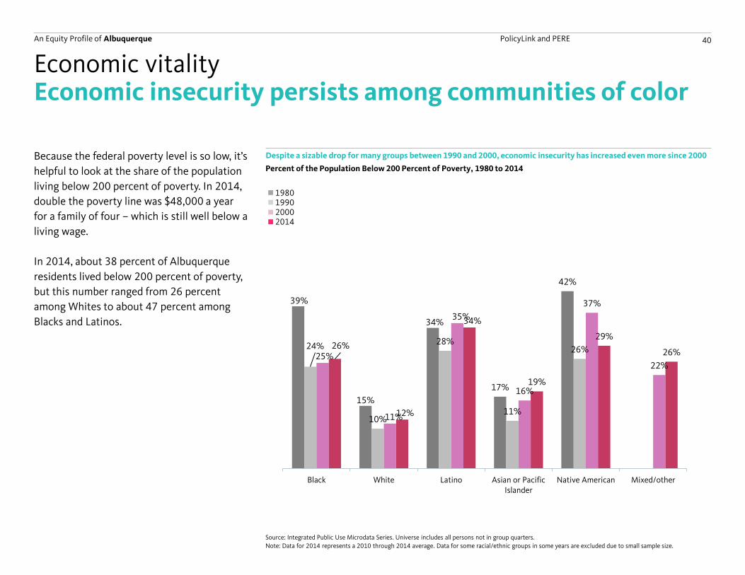
Economic insecurity persists among communities of color
Because the federal poverty level is so low, it’s
helpful to look at the share of the population
living below 200 percent of poverty. In 2014,
double the poverty line was $48,000 a year
for a family of four – which is still well below a
living wage.
In 2014, about 38 percent of Albuquerque
residents lived below 200 percent of poverty,
but this number ranged from 26 percent
among Whites to about 47 percent among
Blacks and Latinos.
Despite a sizable drop for many groups between 1990 and 2000, economic insecurity has increased even more since 2000
Economic vitality
Percent of the Population Below 200 Percent of Poverty, 1980 to 2014
Source: Integrated Public Use Microdata Series. Universe includes all persons not in group quarters.
Note: Data for 2014 represents a 2010 through 2014 average. Data for some racial/ethnic groups in some years are excluded due to small sample size.
21%
45% 46%51% 50%
23%
45%47%
30%
59%
20%
41%43%
24%
53%
32%
26%
47% 47%
36%
59%
42%
White Black Latino Asian orPacific Islander
Native American Mixed/other
1980199020002014
An Equity Profile of Albuquerque PolicyLink and PERE 41
14.4%
8.9%7.9%
7.2%
3.5%
9.4%
7.3% 7.1%
4.0%
14.7%
9.3%
6.7%7.8%
2.3%
14.7%
8.6% 8.3%
7.4%
2.7%
Less than aHS Diploma
HS Diploma,no College
Some College,no Degree
AA Degree,no BA
BA Degreeor higher
0.0%
2.0%
4.0%
6.0%
8.0%
10.0%
12.0%
14.0%
16.0%
Less than aHS Diploma
HS Diploma,no College
Some College,no Degree
AA Degree,no BA
BA Degreeor higher
AllWhiteLatinoPeople of Color
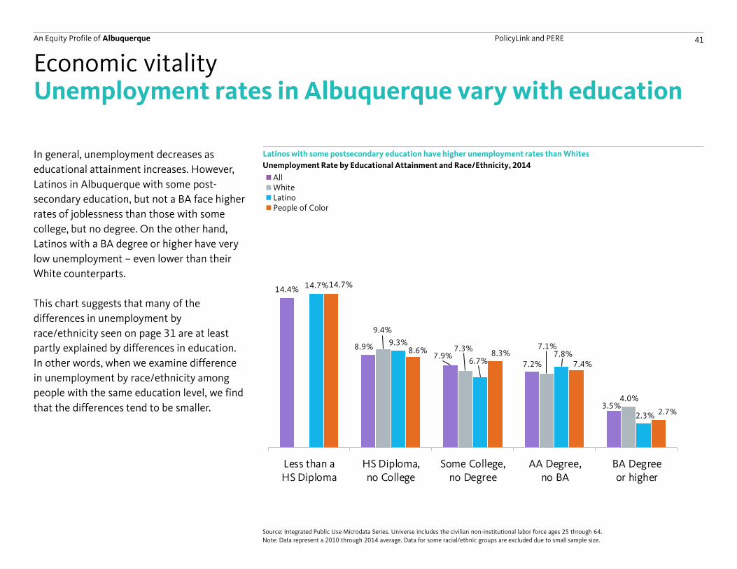
Unemployment rates in Albuquerque vary with education
In general, unemployment decreases as
educational attainment increases. However,
Latinos in Albuquerque with some post-
secondary education, but not a BA face higher
rates of joblessness than those with some
college, but no degree. On the other hand,
Latinos with a BA degree or higher have very
low unemployment – even lower than their
White counterparts.
This chart suggests that many of the
differences in unemployment by
race/ethnicity seen on page 31 are at least
partly explained by differences in education.
In other words, when we examine difference
in unemployment by race/ethnicity among
people with the same education level, we find
that the differences tend to be smaller.
Latinos with some postsecondary education have higher unemployment rates than Whites
Economic vitality
Unemployment Rate by Educational Attainment and Race/Ethnicity, 2014
Source: Integrated Public Use Microdata Series. Universe includes the civilian non-institutional labor force ages 25 through 64.
Note: Data represent a 2010 through 2014 average. Data for some racial/ethnic groups are excluded due to small sample size.
An Equity Profile of Albuquerque PolicyLink and PERE 42
$11.60
$15.50
$18.30 $20.00
$27.40
$17.30 $19.20
$21.40
$29.10
$11.60
$15.30
$17.00
$19.70 $25.00
$11.60
$14.90
$16.90
$18.50
$24.70
Less than aHS Diploma
HS Diploma,no College
Some College,no Degree
AA Degree,no BA
BA Degreeor higher
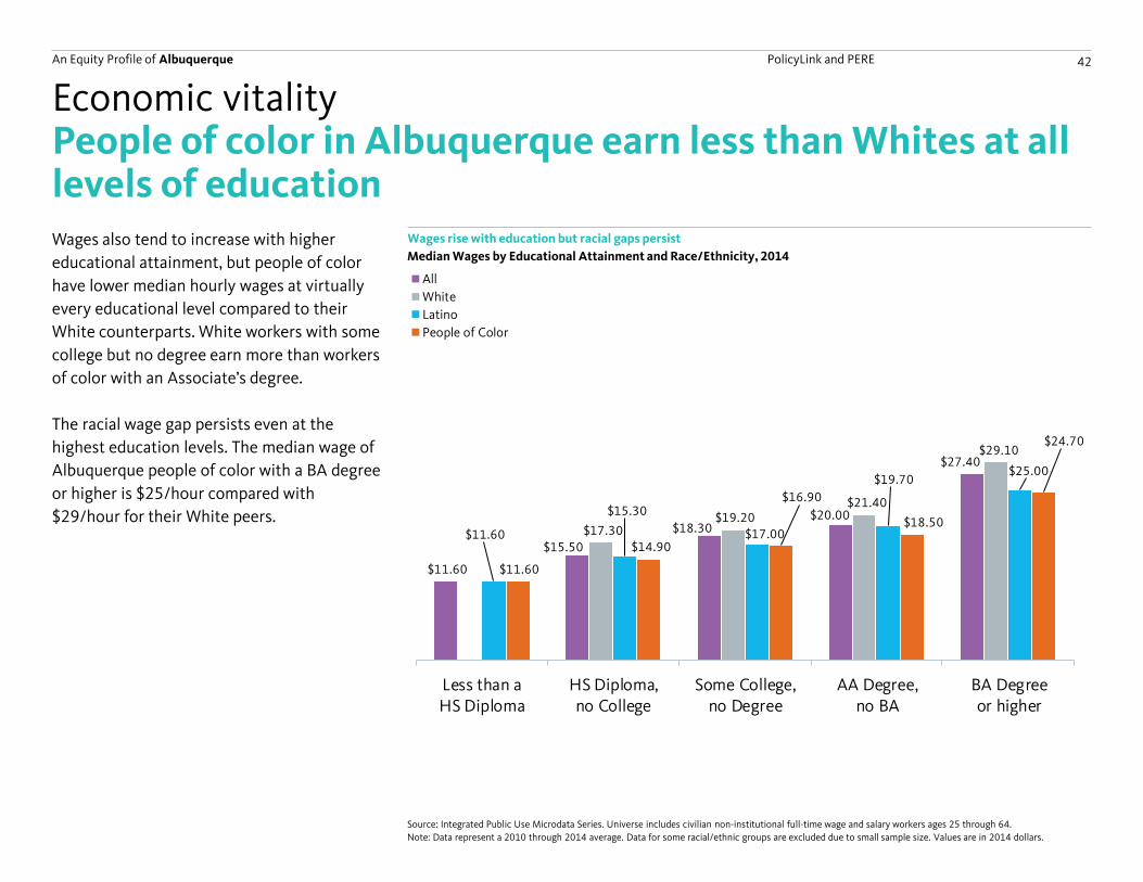
People of color in Albuquerque earn less than Whites at all levels of educationWages also tend to increase with higher
educational attainment, but people of color
have lower median hourly wages at virtually
every educational level compared to their
White counterparts. White workers with some
college but no degree earn more than workers
of color with an Associate’s degree.
The racial wage gap persists even at the
highest education levels. The median wage of
Albuquerque people of color with a BA degree
or higher is $25/hour compared with
$29/hour for their White peers.
Wages rise with education but racial gaps persist
Economic vitality
Median Wages by Educational Attainment and Race/Ethnicity, 2014
Source: Integrated Public Use Microdata Series. Universe includes civilian non-institutional full-time wage and salary workers ages 25 through 64.
Note: Data represent a 2010 through 2014 average. Data for some racial/ethnic groups are excluded due to small sample size. Values are in 2014 dollars.
$0
$10
$20
$30
$40
Less than aHS Diploma
HS Diploma,no College
Some College,no Degree
AA Degree,no BA
BA Degreeor higher
All
White
Latino
People of Color
An Equity Profile of Albuquerque PolicyLink and PERE 43
10.5%
6.8%
3.3%
7.9%
7.7%
4.7%
12.5%
10.4%
7.2%
1.5%
18.4%
6.5%
8.9%
3.8%
Less than aHS Diploma
HS Diploma,no College
More than HS Diploma,Less than BA
BA Degreeor higher
0.0%
10.5%
6.8%
3.3%
0.0%
7.9%
7.7%
4.7%
12.5%
10.4%
7.2%
1.5%
18.4%
6.5%
8.9%
3.8%
Less than aHS Diploma
HS Diploma,no College
More than HS Diploma,Less than BA
BA Degreeor higher
Women of colorMen of colorWhite womenWhite men
$18.70
$20.40
$32.70
$15.50
$18.70
$26.00
$13.10
$16.80
$19.40
$27.40
$13.30
$15.80
$22.20
Less than aHS Diploma
HS Diploma,no College
More than HS Diploma,Less than BA
BA Degreeor higher
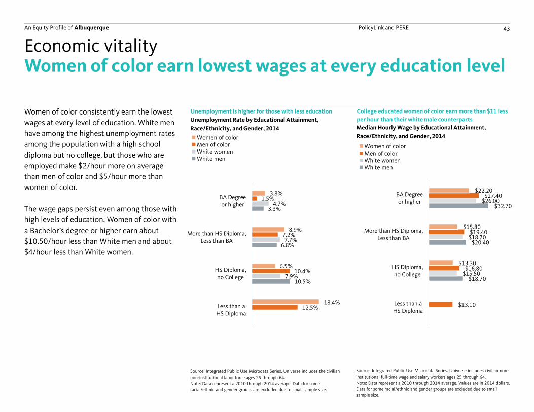
Women of color earn lowest wages at every education level
Women of color consistently earn the lowest
wages at every level of education. White men
have among the highest unemployment rates
among the population with a high school
diploma but no college, but those who are
employed make $2/hour more on average
than men of color and $5/hour more than
women of color.
The wage gaps persist even among those with
high levels of education. Women of color with
a Bachelor’s degree or higher earn about
$10.50/hour less than White men and about
$4/hour less than White women.
Unemployment is higher for those with less education
Economic vitality
Unemployment Rate by Educational Attainment,
Race/Ethnicity, and Gender, 2014
Source: Integrated Public Use Microdata Series. Universe includes civilian non-
institutional full-time wage and salary workers ages 25 through 64.
Note: Data represent a 2010 through 2014 average. Values are in 2014 dollars.
Data for some racial/ethnic and gender groups are excluded due to small
sample size.
Source: Integrated Public Use Microdata Series. Universe includes the civilian
non-institutional labor force ages 25 through 64.
Note: Data represent a 2010 through 2014 average. Data for some
racial/ethnic and gender groups are excluded due to small sample size.
Median Hourly Wage by Educational Attainment,
Race/Ethnicity, and Gender, 2014
College educated women of color earn more than $11 less
per hour than their white male counterparts
0.0%
10.5%
6.8%
3.3%
0.0%
7.9%
7.7%
4.7%
12.5%
10.4%
7.2%
1.5%
18.4%
6.5%
8.9%
3.8%
Less than aHS Diploma
HS Diploma,no College
More than HS Diploma,Less than BA
BA Degreeor higher
Women of colorMen of colorWhite womenWhite men
An Equity Profile of Albuquerque PolicyLink and PERE 44
45%
31%31%
14%13%
19%
Jobs Earnings per worker
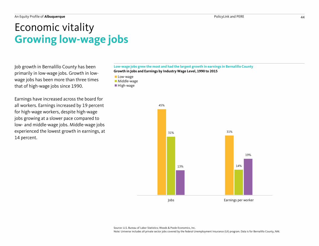
Growing low-wage jobs
Job growth in Bernalillo County has been
primarily in low-wage jobs. Growth in low-
wage jobs has been more than three times
that of high-wage jobs since 1990.
Earnings have increased across the board for
all workers. Earnings increased by 19 percent
for high-wage workers, despite high-wage
jobs growing at a slower pace compared to
low- and middle-wage jobs. Middle-wage jobs
experienced the lowest growth in earnings, at
14 percent.
Low-wage jobs grew the most and had the largest growth in earnings in Bernalillo County
Economic vitality
Growth in Jobs and Earnings by Industry Wage Level, 1990 to 2015
Source: U.S. Bureau of Labor Statistics; Woods & Poole Economics, Inc.
Note: Universe includes all private sector jobs covered by the federal Unemployment Insurance (UI) program. Data is for Bernalillo County, NM.
45%
31%31%
14%13%
19%
Jobs Earnings per worker
Low-wageMiddle-wageHigh-wage
An Equity Profile of Albuquerque PolicyLink and PERE 45
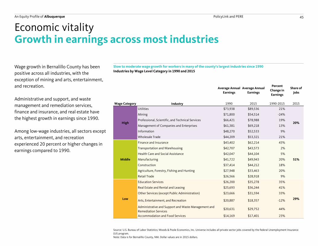
Wage growth in Bernalillo County has been
positive across all industries, with the
exception of mining and arts, entertainment,
and recreation.
Administrative and support, and waste
management and remediation services,
finance and insurance, and real estate have
the highest growth in earnings since 1990.
Among low-wage industries, all sectors except
arts, entertainment, and recreation
experienced 20 percent or higher changes in
earnings compared to 1990.
Growth in earnings across most industries
Slow to moderate wage growth for workers in many of the county’s largest industries since 1990
Economic vitality
Industries by Wage Level Category in 1990 and 2015
Source: U.S. Bureau of Labor Statistics; Woods & Poole Economics, Inc. Universe includes all private sector jobs covered by the federal Unemployment Insurance
(UI) program.
Note: Data is for Bernalillo County, NM. Dollar values are in 2015 dollars.
Average Annual
Earnings
Average Annual
Earnings
Percent
Change in
Earnings
Share of
Jobs
Wage Category Industry 1990 2015 1990-2015 2015
Utilities $73,938 $89,536 21%
Mining $71,800 $54,514 -24%
Professional, Scientific, and Technical Services $66,421 $78,988 19%
Management of Companies and Enterprises $61,381 $69,218 13%
Information $48,270 $52,533 9%
Wholesale Trade $44,209 $53,321 21%
Finance and Insurance $43,402 $62,214 43%
Transportation and Warehousing $42,707 $43,573 2%
Health Care and Social Assistance $42,047 $44,104 5%
Manufacturing $41,722 $49,943 20%
Construction $37,414 $44,212 18%
Agriculture, Forestry, Fishing and Hunting $27,948 $33,463 20%
Retail Trade $26,566 $28,918 9%
Education Services $26,200 $35,278 35%
Real Estate and Rental and Leasing $25,693 $36,244 41%
Other Services (except Public Administration) $23,666 $31,594 33%
Arts, Entertainment, and Recreation $20,887 $18,357 -12%
Administrative and Support and Waste Management and
Remediation Services$20,631 $29,752 44%
Accommodation and Food Services $14,169 $17,401 23%
Low 29%
High 20%
Middle 51%
An Equity Profile of Grand Rapids PolicyLink and PERE 46
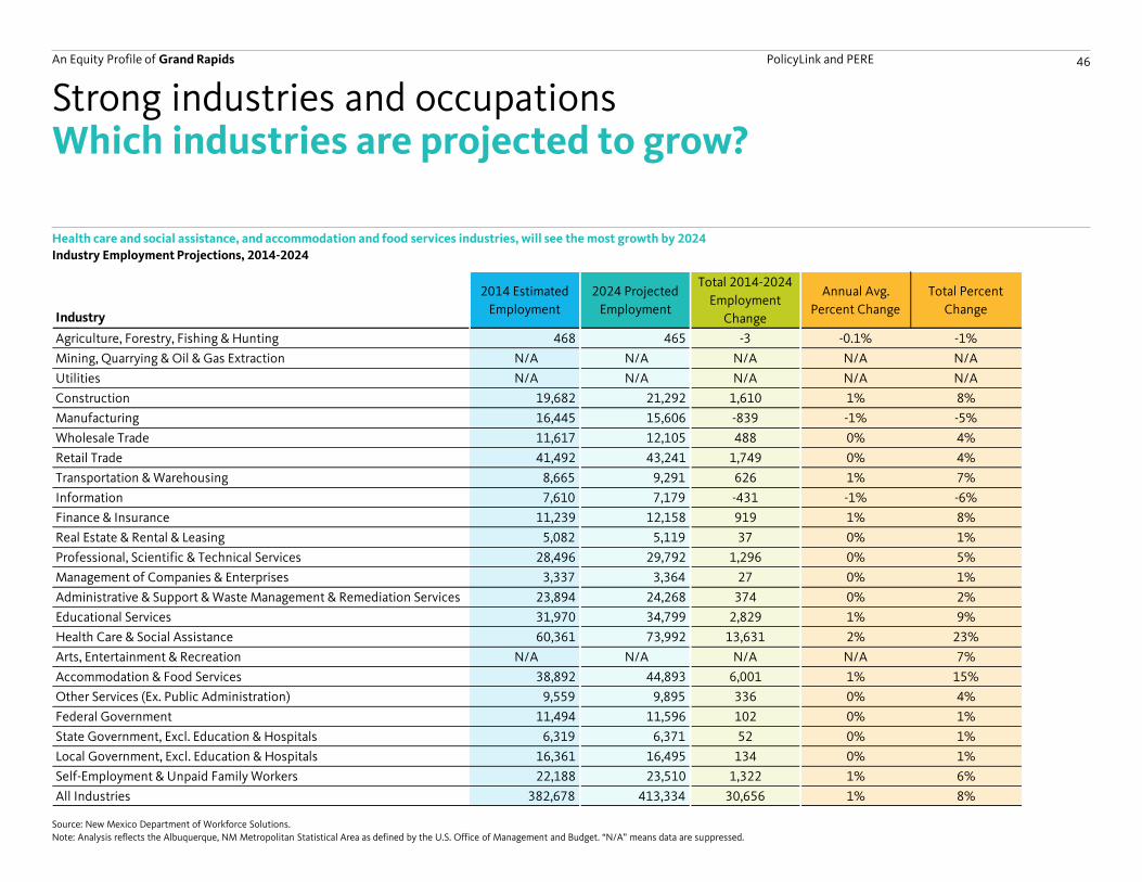
Strong industries and occupationsWhich industries are projected to grow?
Health care and social assistance, and accommodation and food services industries, will see the most growth by 2024
Industry Employment Projections, 2014-2024
Source: New Mexico Department of Workforce Solutions.
Note: Analysis reflects the Albuquerque, NM Metropolitan Statistical Area as defined by the U.S. Office of Management and Budget. “N/A” means data are suppressed.
Industry
2014 Estimated
Employment
2024 Projected
Employment
Total 2014-2024
Employment
Change
Annual Avg.
Percent Change
Total Percent
Change
Agriculture, Forestry, Fishing & Hunting 468 465 -3 -0.1% -1%
Mining, Quarrying & Oil & Gas Extraction N/A N/A N/A N/A N/A
Utilities N/A N/A N/A N/A N/A
Construction 19,682 21,292 1,610 1% 8%
Manufacturing 16,445 15,606 -839 -1% -5%
Wholesale Trade 11,617 12,105 488 0% 4%
Retail Trade 41,492 43,241 1,749 0% 4%
Transportation & Warehousing 8,665 9,291 626 1% 7%
Information 7,610 7,179 -431 -1% -6%
Finance & Insurance 11,239 12,158 919 1% 8%
Real Estate & Rental & Leasing 5,082 5,119 37 0% 1%
Professional, Scientific & Technical Services 28,496 29,792 1,296 0% 5%
Management of Companies & Enterprises 3,337 3,364 27 0% 1%
Administrative & Support & Waste Management & Remediation Services 23,894 24,268 374 0% 2%
Educational Services 31,970 34,799 2,829 1% 9%
Health Care & Social Assistance 60,361 73,992 13,631 2% 23%
Arts, Entertainment & Recreation N/A N/A N/A N/A 7%
Accommodation & Food Services 38,892 44,893 6,001 1% 15%
Other Services (Ex. Public Administration) 9,559 9,895 336 0% 4%
Federal Government 11,494 11,596 102 0% 1%
State Government, Excl. Education & Hospitals 6,319 6,371 52 0% 1%
Local Government, Excl. Education & Hospitals 16,361 16,495 134 0% 1%
Self-Employment & Unpaid Family Workers 22,188 23,510 1,322 1% 6%
All Industries 382,678 413,334 30,656 1% 8%
An Equity Profile of Grand Rapids PolicyLink and PERE 47
Occupation
2014 Estimated
Employment
2024
Projected
Employment
Total 2014-
2024
Employment
Change
Annual Avg.
Percent
Change
Total
Percent
Change
Management Occupations 21,284 22,693 1,409 0.6% 7%
Business & Financial Operations Occupations 18,876 20,155 1,279 0.7% 7%
Computer & Mathematical Occupations 9,034 9,619 585 0.6% 6%
Architecture & Engineering Occupations 12,430 12,550 120 0.1% 1%
Life, Physical & Social Science Occupations 4,144 4,429 285 0.7% 7%
Community & Social Service Occupations 6,621 7,423 802 1.1% 12%
Legal Occupations 3,600 3,630 30 0.1% 1%
Education, Training & Library Occupations 22,319 24,666 2,347 1.0% 11%
Arts, Design, Entertainment, Sports & Media Occupations 5,355 5,617 262 0.5% 5%
Healthcare Practitioners & Technical Occupations 25,398 29,770 4,372 1.6% 17%
Healthcare Support Occupations 12,993 15,582 2,589 1.8% 20%
Protective Service Occupations 9,185 9,421 236 0.3% 3%
Food Preparation & Serving Related Occupations 36,198 41,439 5,241 1.4% 14%
Building & Grounds Cleaning & Maintenance Occupations 13,649 14,302 653 0.5% 5%
Personal Care & Service Occupations 17,968 22,458 4,490 2.3% 25%
Sales & Related Occupations 39,855 41,669 1,814 0.4% 5%
Office & Administrative Support Occupations 57,394 58,469 1,075 0.2% 2%
Farming, Fishing & Forestry Occupations 478 463 -15 -0.3% -3%
Construction & Extraction Occupations 21,185 22,587 1,402 0.6% 7%
Installation, Maintenance & Repair Occupations 13,559 14,089 530 0.4% 4%
Production Occupations 11,108 11,003 -105 -0.1% -1%
Transportation & Material Moving Occupations 20,045 21,300 1,255 0.6% 6%
All Occupations 382,678 413,334 30,656 0.8% 8%
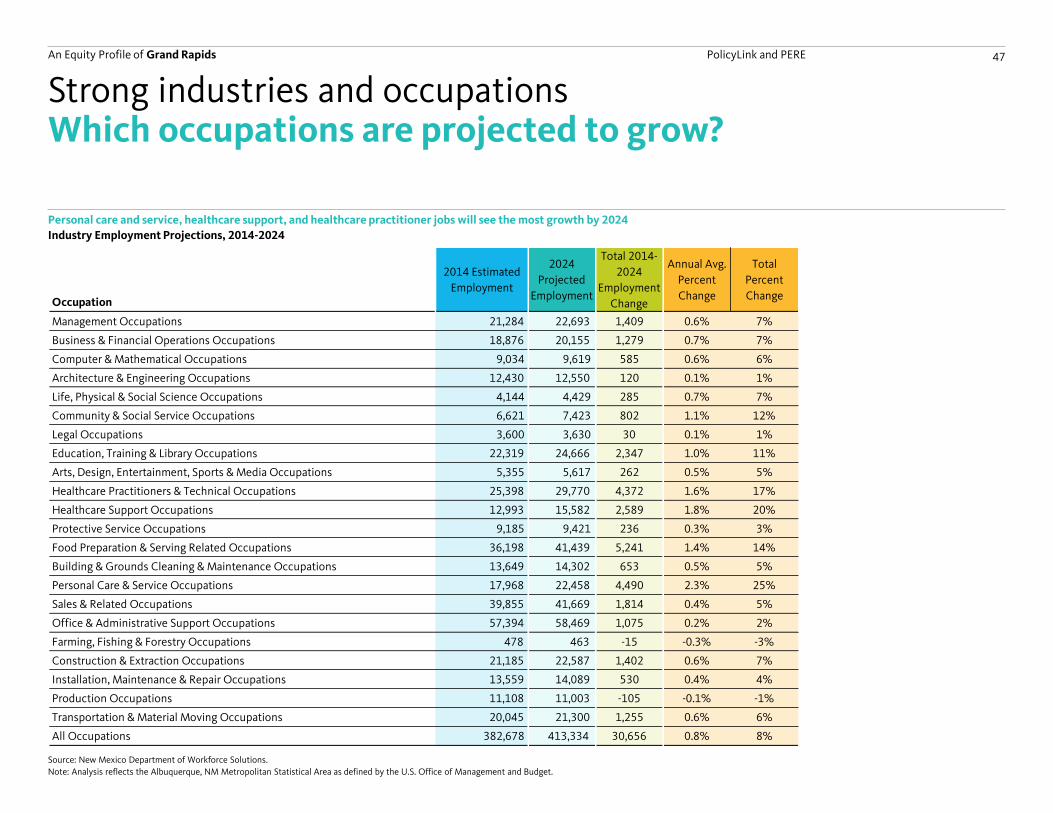
Strong industries and occupationsWhich occupations are projected to grow?
Personal care and service, healthcare support, and healthcare practitioner jobs will see the most growth by 2024
Industry Employment Projections, 2014-2024
Source: New Mexico Department of Workforce Solutions.
Note: Analysis reflects the Albuquerque, NM Metropolitan Statistical Area as defined by the U.S. Office of Management and Budget.
An Equity Profile of Albuquerque PolicyLink and PERE 48
Size + Concentration + Job quality + Growth(2012) (2012) (2012) (2002-2012)
Industry strength index =
Total Employment
The total number of jobs
in a particular industry.
Location Quotient
A measure of employment
concentration calculated by
dividing the share of
employment for a particular
industry in the region by its
share nationwide. A score
>1 indicates higher-than-
average concentration.
Average Annual Wage
The estimated total
annual wages of an
industry divided by its
estimated total
employment.
Change in the number
of jobs
Percent change in the
number of jobs
Real wage growth
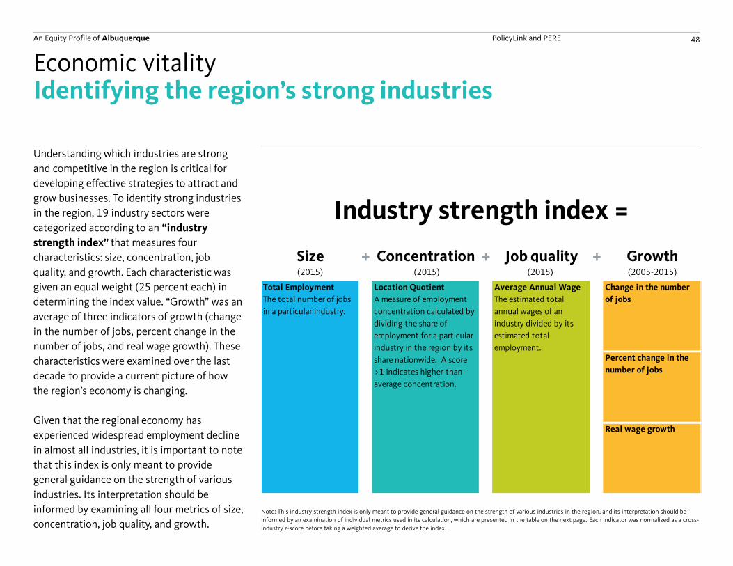
Identifying the region’s strong industries
Understanding which industries are strong
and competitive in the region is critical for
developing effective strategies to attract and
grow businesses. To identify strong industries
in the region, 19 industry sectors were
categorized according to an “industry
strength index” that measures four
characteristics: size, concentration, job
quality, and growth. Each characteristic was
given an equal weight (25 percent each) in
determining the index value. “Growth” was an
average of three indicators of growth (change
in the number of jobs, percent change in the
number of jobs, and real wage growth). These
characteristics were examined over the last
decade to provide a current picture of how
the region’s economy is changing.
Given that the regional economy has
experienced widespread employment decline
in almost all industries, it is important to note
that this index is only meant to provide
general guidance on the strength of various
industries. Its interpretation should be
informed by examining all four metrics of size,
concentration, job quality, and growth.
Economic vitality
Note: This industry strength index is only meant to provide general guidance on the strength of various industries in the region, and its interpretation should be
informed by an examination of individual metrics used in its calculation, which are presented in the table on the next page. Each indicator was normalized as a cross-
industry z-score before taking a weighted average to derive the index.
(2015) (2015) (2015) (2005-2015)
An Equity Profile of Albuquerque PolicyLink and PERE 49
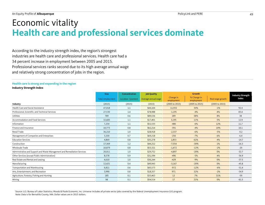
Size Concentration Job Quality
Total employment Location Quotient Average annual wageChange in
employment
% Change in
employmentReal wage growth
Industry (2015) (2015) (2015) (2005 to 2015) (2005 to 2015) (2005 to 2015)
Health Care and Social Assistance 47,018 1.1 $44,104 11,932 34% -1% 92.4
Professional, Scientific, and Technical Services 27,530 1.4 $78,988 -1,195 -4% 4% 83.4
Utilities 789 0.6 $89,536 289 58% 8% 38
Accommodation and Food Services 32,683 1.1 $17,401 3,195 11% 5% 12.9
Information 7,234 1.1 $52,533 -480 -6% 12% 11.7
Finance and Insurance 10,773 0.8 $62,214 -391 -4% 10% 10.1
Retail Trade 36,210 1.0 $28,918 -2,337 -6% -5% -0.2
Management of Companies and Enterprises 3,330 0.7 $69,218 -250 -7% 6% -6.4
Education Services 4,869 0.8 $35,278 1,853 61% 4% -14.7
Construction 17,369 1.2 $44,212 -7,554 -30% 1% -16.3
Wholesale Trade 10,879 0.8 $53,321 -1,472 -12% -2% -20
Administrative and Support and Waste Management and Remediation Services 20,011 1.0 $29,752 -4,897 -20% 0% -32.7
Other Services (except Public Administration) 8,578 0.9 $31,594 -496 -5% 4% -36.9
Real Estate and Rental and Leasing 4,610 1.0 $36,244 -429 -9% 0% -37.5
Manufacturing 12,421 0.4 $49,943 -3,167 -20% 0% -45.8
Transportation and Warehousing 6,811 0.6 $43,573 -972 -12% -6% -51.4
Arts, Entertainment, and Recreation 3,990 0.8 $18,357 971 32% -2% -54.9
Agriculture, Forestry, Fishing and Hunting 185 0.1 $33,463 12 7% 31% -59
Mining 98 0.1 $54,514 17 21% 0% -61.5
Growth Industry Strength
Index
According to the industry strength index, the region’s strongest
industries are health care and professional services. Health care had a
34 percent increase in employment between 2005 and 2015.
Professional services ranks second due to its high average annual wage
and relatively strong concentration of jobs in the region.
Health care and professional services dominate
Health care is strong and expanding in the region
Economic vitality
Industry Strength Index
Source: U.S. Bureau of Labor Statistics; Woods & Poole Economic, Inc. Universe includes all private sector jobs covered by the federal Unemployment Insurance (UI) program.
Note: Data is for Bernalillo County, NM. Dollar values are in 2015 dollars.
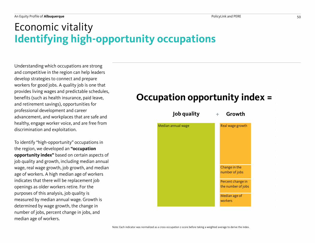
An Equity Profile of Albuquerque PolicyLink and PERE 50
+ Growth
Median annual wage Real wage growth
Change in the
number of jobs
Percent change in
the number of jobs
Median age of
workers
Occupation opportunity index =
Job quality
Identifying high-opportunity occupations
Understanding which occupations are strong
and competitive in the region can help leaders
develop strategies to connect and prepare
workers for good jobs. A quality job is one that
provides living wages and predictable schedules,
benefits (such as health insurance, paid leave,
and retirement savings), opportunities for
professional development and career
advancement, and workplaces that are safe and
healthy, engage worker voice, and are free from
discrimination and exploitation.
To identify “high-opportunity” occupations in
the region, we developed an “occupation
opportunity index” based on certain aspects of
job quality and growth, including median annual
wage, real wage growth, job growth, and median
age of workers. A high median age of workers
indicates that there will be replacement job
openings as older workers retire. For the
purposes of this analysis, job quality is
measured by median annual wage. Growth is
determined by wage growth, the change in
number of jobs, percent change in jobs, and
median age of workers.
Economic vitality
Note: Each indicator was normalized as a cross-occupation z-score before taking a weighted average to derive the index.
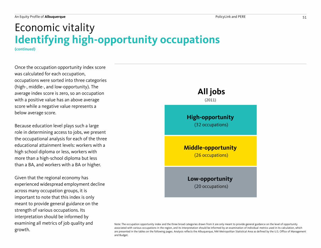
An Equity Profile of Albuquerque PolicyLink and PERE 51
Identifying high-opportunity occupations
Once the occupation opportunity index score
was calculated for each occupation,
occupations were sorted into three categories
(high-, middle-, and low-opportunity). The
average index score is zero, so an occupation
with a positive value has an above average
score while a negative value represents a
below average score.
Because education level plays such a large
role in determining access to jobs, we present
the occupational analysis for each of the three
educational attainment levels: workers with a
high school diploma or less, workers with
more than a high-school diploma but less
than a BA, and workers with a BA or higher.
Given that the regional economy has
experienced widespread employment decline
across many occupation groups, it is
important to note that this index is only
meant to provide general guidance on the
strength of various occupations. Its
interpretation should be informed by
examining all metrics of job quality and
growth.
Economic vitality
(continued)
Note: The occupation opportunity index and the three broad categories drawn from it are only meant to provide general guidance on the level of opportunity
associated with various occupations in the region, and its interpretation should be informed by an examination of individual metrics used in its calculation, which
are presented in the tables on the following pages. Analysis reflects the Albuquerque, NM Metropolitan Statistical Area as defined by the U.S. Office of Management
and Budget.
High-opportunity(32 occupations)
Middle-opportunity(26 occupations)
Low-opportunity(20 occupations)
All jobs(2011)
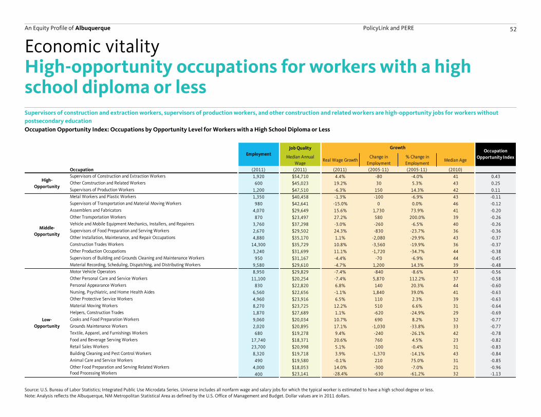
An Equity Profile of Albuquerque PolicyLink and PERE 52
Job Quality
Median Annual
WageReal Wage Growth
Change in
Employment
% Change in
EmploymentMedian Age
Occupation (2011) (2011) (2011) (2005-11) (2005-11) (2010)
Supervisors of Construction and Extraction Workers 1,920 $54,710 4.4% -80 -4.0% 41 0.43
Other Construction and Related Workers 600 $45,023 19.2% 30 5.3% 43 0.25
Supervisors of Production Workers 1,200 $47,510 -6.3% 150 14.3% 42 0.11
Metal Workers and Plastic Workers 1,350 $40,458 -1.3% -100 -6.9% 43 -0.11
Supervisors of Transportation and Material Moving Workers 980 $42,641 -15.0% 0 0.0% 46 -0.12
Assemblers and Fabricators 4,070 $29,649 15.6% 1,730 73.9% 41 -0.20
Other Transportation Workers 870 $23,497 27.2% 580 200.0% 39 -0.26
Vehicle and Mobile Equipment Mechanics, Installers, and Repairers 3,760 $37,298 -3.0% -260 -6.5% 40 -0.26
Supervisors of Food Preparation and Serving Workers 2,670 $29,502 24.3% -830 -23.7% 36 -0.36
Other Installation, Maintenance, and Repair Occupations 4,880 $35,170 1.1% -2,080 -29.9% 43 -0.37
Construction Trades Workers 14,300 $35,729 10.8% -3,560 -19.9% 36 -0.37
Other Production Occupations 3,240 $31,699 11.1% -1,720 -34.7% 44 -0.38
Supervisors of Building and Grounds Cleaning and Maintenance Workers 950 $31,167 -4.4% -70 -6.9% 44 -0.45
Material Recording, Scheduling, Dispatching, and Distributing Workers 9,580 $29,610 -4.7% 1,200 14.3% 39 -0.48
Motor Vehicle Operators 8,950 $29,829 -7.4% -840 -8.6% 43 -0.56
Other Personal Care and Service Workers 11,100 $20,254 -7.4% 5,870 112.2% 37 -0.58
Personal Appearance Workers 830 $22,820 6.8% 140 20.3% 44 -0.60
Nursing, Psychiatric, and Home Health Aides 6,560 $22,656 -1.1% 1,840 39.0% 41 -0.63
Other Protective Service Workers 4,960 $23,916 6.5% 110 2.3% 39 -0.63
Material Moving Workers 8,270 $23,725 12.2% 510 6.6% 31 -0.64
Helpers, Construction Trades 1,870 $27,689 1.1% -620 -24.9% 29 -0.69
Cooks and Food Preparation Workers 9,060 $20,034 10.7% 690 8.2% 32 -0.77
Grounds Maintenance Workers 2,020 $20,895 17.1% -1,030 -33.8% 33 -0.77
Textile, Apparel, and Furnishings Workers 680 $19,278 9.4% -240 -26.1% 42 -0.78
Food and Beverage Serving Workers 17,740 $18,371 20.6% 760 4.5% 23 -0.82
Retail Sales Workers 23,700 $20,998 5.1% -100 -0.4% 31 -0.83
Building Cleaning and Pest Control Workers 8,320 $19,718 3.9% -1,370 -14.1% 43 -0.84
Animal Care and Service Workers 490 $19,580 -0.1% 210 75.0% 31 -0.85
Other Food Preparation and Serving Related Workers 4,000 $18,053 14.0% -300 -7.0% 21 -0.96Food Processing Workers 400 $23,141 -28.4% -630 -61.2% 32 -1.13
Low-
Opportunity
Employment
GrowthOccupation
Opportunity Index
High-
Opportunity
Middle-
Opportunity
High-opportunity occupations for workers with a high school diploma or lessSupervisors of construction and extraction workers, supervisors of production workers, and other construction and related workers are high-opportunity jobs for workers without
postsecondary education
Economic vitality
Occupation Opportunity Index: Occupations by Opportunity Level for Workers with a High School Diploma or Less
Source: U.S. Bureau of Labor Statistics; Integrated Public Use Microdata Series. Universe includes all nonfarm wage and salary jobs for which the typical worker is estimated to have a high school degree or less.
Note: Analysis reflects the Albuquerque, NM Metropolitan Statistical Area as defined by the U.S. Office of Management and Budget. Dollar values are in 2011 dollars.
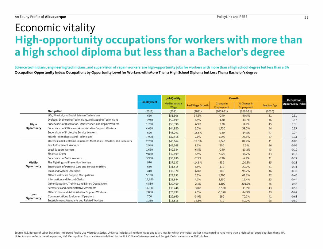
An Equity Profile of Albuquerque PolicyLink and PERE 53
Job Quality
Median Annual
WageReal Wage Growth
Change in
Employment
% Change in
EmploymentMedian Age
Occupation (2011) (2011) (2011) (2005-11) (2005-11) (2010)
Life, Physical, and Social Science Technicians 660 $51,506 39.5% -290 -30.5% 31 0.51
Drafters, Engineering Technicians, and Mapping Technicians 3,940 $52,699 3.8% -680 -14.7% 46 0.37
Supervisors of Installation, Maintenance, and Repair Workers 1,230 $53,390 -6.9% -120 -8.9% 45 0.31
Supervisors of Office and Administrative Support Workers 4,660 $44,920 6.0% 1,730 59.0% 44 0.25
Supervisors of Protective Service Workers 690 $48,291 -15.5% -120 -14.8% 47 0.07
Health Technologists and Technicians 7,990 $42,516 2.1% 1,690 26.8% 37 0.04
Electrical and Electronic Equipment Mechanics, Installers, and Repairers 2,230 $43,664 -19.3% 1,040 87.4% 41 -0.05
Law Enforcement Workers 2,940 $42,368 1.1% 200 7.3% 36 -0.06
Legal Support Workers 1,650 $42,384 -6.5% -250 -13.2% 43 -0.10
Financial Clerks 9,860 $32,499 7.5% 2,620 36.2% 43 -0.16
Supervisors of Sales Workers 3,960 $36,880 -2.3% -290 -6.8% 41 -0.27
Fire Fighting and Prevention Workers 970 $37,137 -14.8% 530 120.5% 35 -0.28
Supervisors of Personal Care and Service Workers 660 $31,515 8.5% 110 20.0% 41 -0.31
Plant and System Operators 410 $30,370 -6.8% 200 95.2% 46 -0.38
Other Healthcare Support Occupations 5,130 $29,751 5.3% 1,700 49.6% 32 -0.40
Information and Record Clerks 17,640 $28,844 4.2% 2,350 15.4% 33 -0.44
Other Education, Training, and Library Occupations 4,880 $20,469 -2.3% 3,300 208.9% 45 -0.47
Secretaries and Administrative Assistants 11,930 $30,746 -3.8% -1,500 -11.2% 43 -0.53
Other Office and Administrative Support Workers 7,890 $26,292 2.5% -1,320 -14.3% 43 -0.62
Communications Equipment Operators 700 $22,660 -3.9% 290 70.7% 41 -0.68
Entertainment Attendants and Related Workers 1,230 $18,816 12.3% 410 50.0% 28 -0.80
Employment
GrowthOccupation
Opportunity Index
Low-
Opportunity
Middle-
Opportunity
High-
Opportunity
High-opportunity occupations for workers with more than a high school diploma but less than a Bachelor’s degreeScience technicians, engineering technicians, and supervision of repair workers are high-opportunity jobs for workers with more than a high school degree but less than a BA
Economic vitality
Occupation Opportunity Index: Occupations by Opportunity Level for Workers with More Than a High School Diploma but Less Than a Bachelor’s degree
Source: U.S. Bureau of Labor Statistics; Integrated Public Use Microdata Series. Universe includes all nonfarm wage and salary jobs for which the typical worker is estimated to have more than a high school degree but less than a BA.
Note: Analysis reflects the Albuquerque, NM Metropolitan Statistical Area as defined by the U.S. Office of Management and Budget. Dollar values are in 2011 dollars.
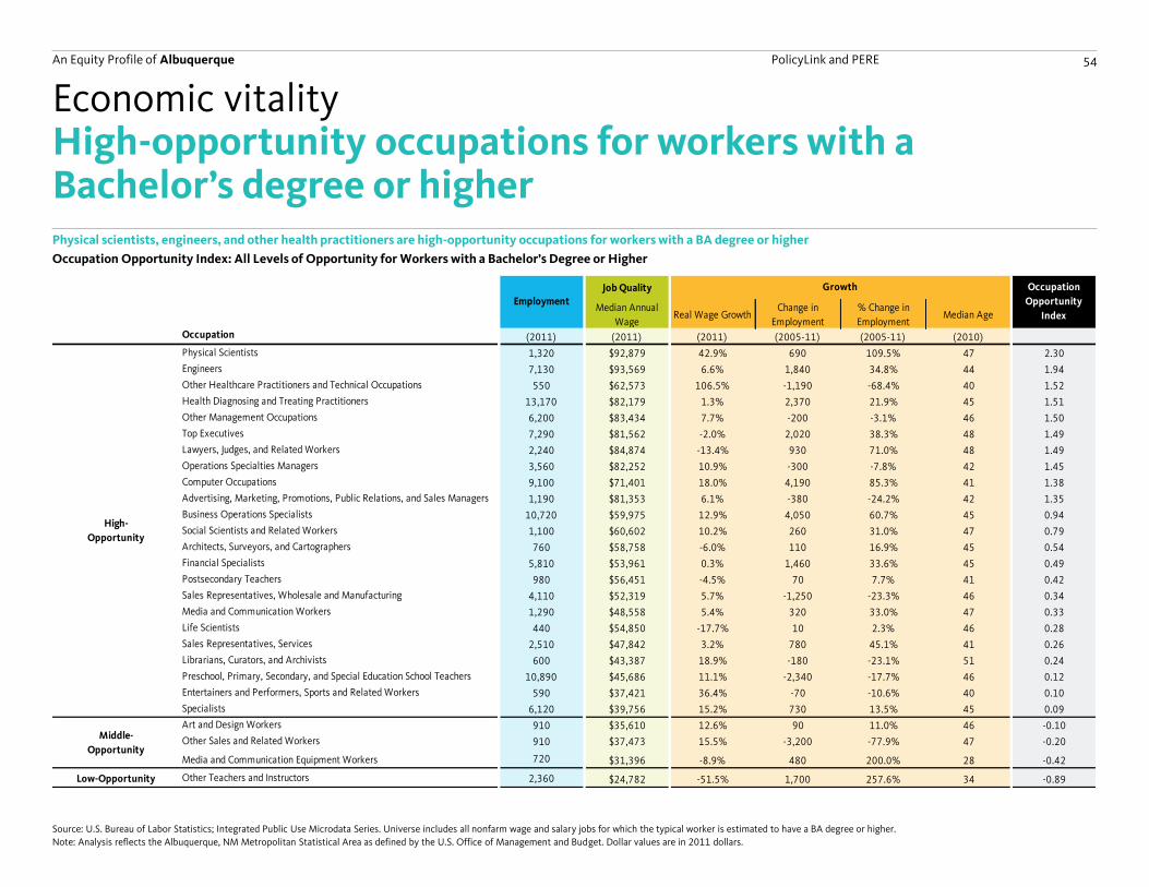
An Equity Profile of Albuquerque PolicyLink and PERE 54
Job Quality
Median Annual
WageReal Wage Growth
Change in
Employment
% Change in
EmploymentMedian Age
Occupation (2011) (2011) (2011) (2005-11) (2005-11) (2010)
Physical Scientists 1,320 $92,879 42.9% 690 109.5% 47 2.30
Engineers 7,130 $93,569 6.6% 1,840 34.8% 44 1.94
Other Healthcare Practitioners and Technical Occupations 550 $62,573 106.5% -1,190 -68.4% 40 1.52
Health Diagnosing and Treating Practitioners 13,170 $82,179 1.3% 2,370 21.9% 45 1.51
Other Management Occupations 6,200 $83,434 7.7% -200 -3.1% 46 1.50
Top Executives 7,290 $81,562 -2.0% 2,020 38.3% 48 1.49
Lawyers, Judges, and Related Workers 2,240 $84,874 -13.4% 930 71.0% 48 1.49
Operations Specialties Managers 3,560 $82,252 10.9% -300 -7.8% 42 1.45
Computer Occupations 9,100 $71,401 18.0% 4,190 85.3% 41 1.38
Advertising, Marketing, Promotions, Public Relations, and Sales Managers 1,190 $81,353 6.1% -380 -24.2% 42 1.35
Business Operations Specialists 10,720 $59,975 12.9% 4,050 60.7% 45 0.94
Social Scientists and Related Workers 1,100 $60,602 10.2% 260 31.0% 47 0.79
Architects, Surveyors, and Cartographers 760 $58,758 -6.0% 110 16.9% 45 0.54
Financial Specialists 5,810 $53,961 0.3% 1,460 33.6% 45 0.49
Postsecondary Teachers 980 $56,451 -4.5% 70 7.7% 41 0.42
Sales Representatives, Wholesale and Manufacturing 4,110 $52,319 5.7% -1,250 -23.3% 46 0.34
Media and Communication Workers 1,290 $48,558 5.4% 320 33.0% 47 0.33
Life Scientists 440 $54,850 -17.7% 10 2.3% 46 0.28
Sales Representatives, Services 2,510 $47,842 3.2% 780 45.1% 41 0.26
Librarians, Curators, and Archivists 600 $43,387 18.9% -180 -23.1% 51 0.24
Preschool, Primary, Secondary, and Special Education School Teachers 10,890 $45,686 11.1% -2,340 -17.7% 46 0.12
Entertainers and Performers, Sports and Related Workers 590 $37,421 36.4% -70 -10.6% 40 0.10Counselors, Social Workers, and Other Community and Social Service
Specialists 6,120 $39,756 15.2% 730 13.5% 45 0.09
Art and Design Workers 910 $35,610 12.6% 90 11.0% 46 -0.10
Other Sales and Related Workers 910 $37,473 15.5% -3,200 -77.9% 47 -0.20
Media and Communication Equipment Workers 720 $31,396 -8.9% 480 200.0% 28 -0.42
Low-Opportunity Other Teachers and Instructors 2,360 $24,782 -51.5% 1,700 257.6% 34 -0.89
Employment
Growth Occupation
Opportunity
Index
High-
Opportunity
Middle-
Opportunity
High-opportunity occupations for workers with a Bachelor’s degree or higherPhysical scientists, engineers, and other health practitioners are high-opportunity occupations for workers with a BA degree or higher
Economic vitality
Occupation Opportunity Index: All Levels of Opportunity for Workers with a Bachelor’s Degree or Higher
Source: U.S. Bureau of Labor Statistics; Integrated Public Use Microdata Series. Universe includes all nonfarm wage and salary jobs for which the typical worker is estimated to have a BA degree or higher.
Note: Analysis reflects the Albuquerque, NM Metropolitan Statistical Area as defined by the U.S. Office of Management and Budget. Dollar values are in 2011 dollars.
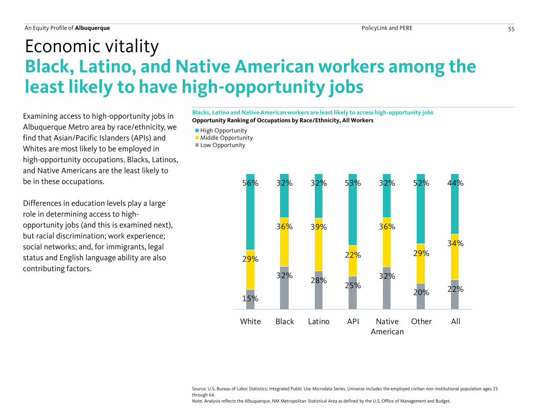
An Equity Profile of Albuquerque PolicyLink and PERE 55
15%
32%28%
25%32%
20% 22%
29%
36% 39%
22%
36%
29%34%
56% 32% 32% 53% 32% 52% 44%
White Black Latino API NativeAmerican
Other All
Black, Latino, and Native American workers among the least likely to have high-opportunity jobs
Examining access to high-opportunity jobs in
Albuquerque Metro area by race/ethnicity, we
find that Asian/Pacific Islanders (APIs) and
Whites are most likely to be employed in
high-opportunity occupations. Blacks, Latinos,
and Native Americans are the least likely to
be in these occupations.
Differences in education levels play a large
role in determining access to high-
opportunity jobs (and this is examined next),
but racial discrimination; work experience;
social networks; and, for immigrants, legal
status and English language ability are also
contributing factors.
Blacks, Latino and Native American workers are least likely to access high-opportunity jobs
Economic vitality
Opportunity Ranking of Occupations by Race/Ethnicity, All Workers
Source: U.S. Bureau of Labor Statistics; Integrated Public Use Microdata Series. Universe includes the employed civilian non-institutional population ages 25
through 64.
Note: Analysis reflects the Albuquerque, NM Metropolitan Statistical Area as defined by the U.S. Office of Management and Budget.
22%
44%38%
31%
34%
30%
47%22%
32%
High OpportunityMiddle OpportunityLow Opportunity
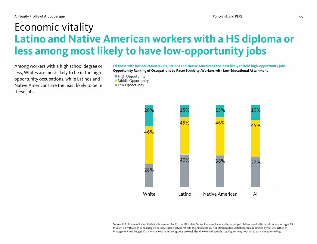
An Equity Profile of Albuquerque PolicyLink and PERE 56
28%
40% 38% 37%
46%
45% 46%45%
26% 15% 15% 19%
White Latino Native American All
22%
44%38%
31%
34%
30%
47%22%
32%
High OpportunityMiddle OpportunityLow Opportunity
Latino and Native American workers with a HS diploma or less among most likely to have low-opportunity jobsAmong workers with a high school degree or
less, Whites are most likely to be in the high-
opportunity occupations, while Latinos and
Native Americans are the least likely to be in
these jobs.
Of those with low education levels, Latinos and Native Americans are least likely to hold high-opportunity jobs
Economic vitality
Opportunity Ranking of Occupations by Race/Ethnicity, Workers with Low Educational Attainment
Source: U.S. Bureau of Labor Statistics; Integrated Public Use Microdata Series. Universe includes the employed civilian non-institutional population ages 25
through 64 with a high school degree or less. Note: Analysis reflects the Albuquerque, NM Metropolitan Statistical Area as defined by the U.S. Office of
Management and Budget. Data for some racial/ethnic groups are excluded due to small sample size. Figures may not sum to total due to rounding.
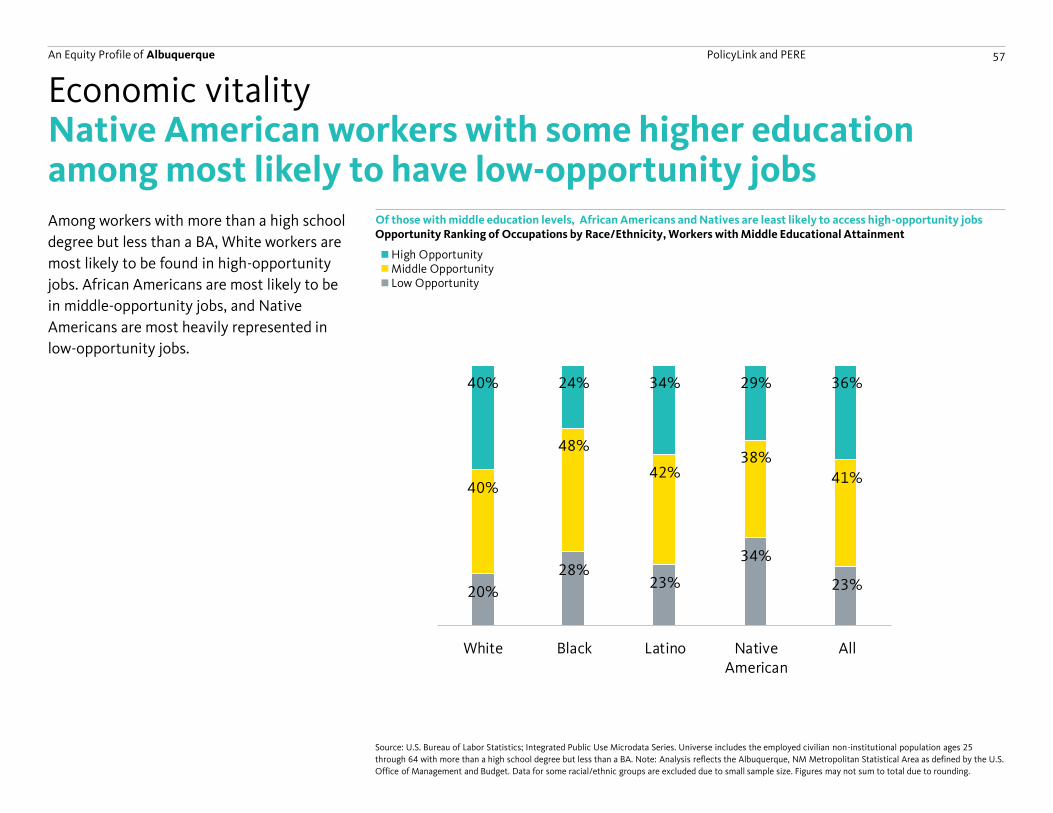
An Equity Profile of Albuquerque PolicyLink and PERE 57
20%
28%23%
34%
23%
40%
48%
42%38%
41%
40% 24% 34% 29% 36%
White Black Latino NativeAmerican
All
22%
44%38%
31%
34%
30%
47%22%
32%
High OpportunityMiddle OpportunityLow Opportunity
Among workers with more than a high school
degree but less than a BA, White workers are
most likely to be found in high-opportunity
jobs. African Americans are most likely to be
in middle-opportunity jobs, and Native
Americans are most heavily represented in
low-opportunity jobs.
Of those with middle education levels, African Americans and Natives are least likely to access high-opportunity jobs
Economic vitality
Opportunity Ranking of Occupations by Race/Ethnicity, Workers with Middle Educational Attainment
Source: U.S. Bureau of Labor Statistics; Integrated Public Use Microdata Series. Universe includes the employed civilian non-institutional population ages 25
through 64 with more than a high school degree but less than a BA. Note: Analysis reflects the Albuquerque, NM Metropolitan Statistical Area as defined by the U.S.
Office of Management and Budget. Data for some racial/ethnic groups are excluded due to small sample size. Figures may not sum to total due to rounding.
Native American workers with some higher education among most likely to have low-opportunity jobs
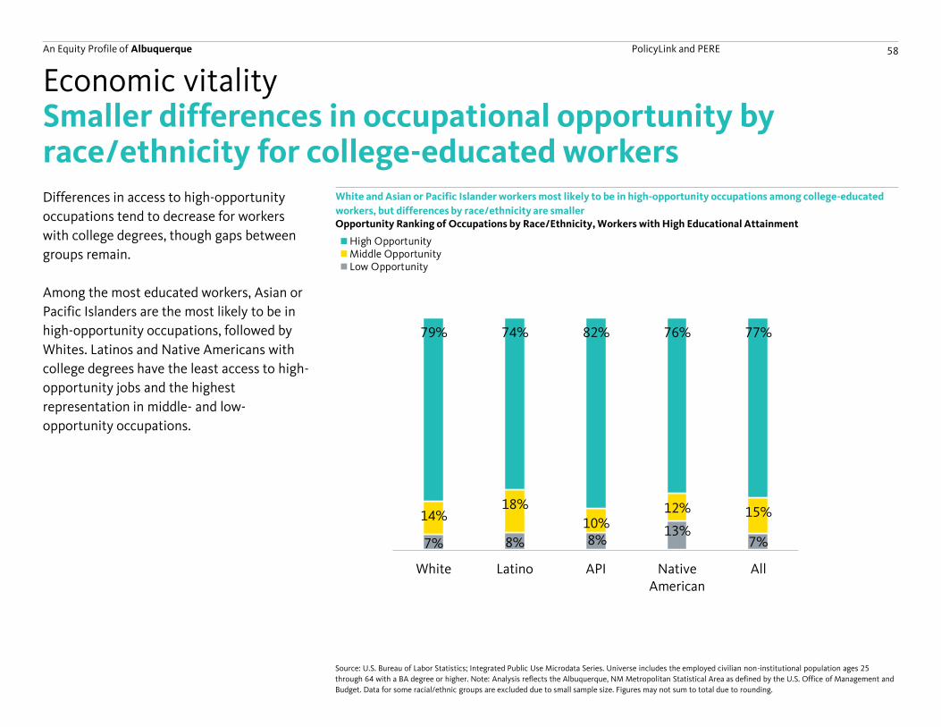
An Equity Profile of Albuquerque PolicyLink and PERE 58
7% 8% 8%13%
7%
14%18%
10%12% 15%
79% 74% 82% 76% 77%
White Latino API NativeAmerican
All
Opportunity Ranking of Occupations by Race/Ethnicity, Workers with High Educational Attainment
Differences in access to high-opportunity
occupations tend to decrease for workers
with college degrees, though gaps between
groups remain.
Among the most educated workers, Asian or
Pacific Islanders are the most likely to be in
high-opportunity occupations, followed by
Whites. Latinos and Native Americans with
college degrees have the least access to high-
opportunity jobs and the highest
representation in middle- and low-
opportunity occupations.
White and Asian or Pacific Islander workers most likely to be in high-opportunity occupations among college-educated
workers, but differences by race/ethnicity are smaller
Economic vitality
Source: U.S. Bureau of Labor Statistics; Integrated Public Use Microdata Series. Universe includes the employed civilian non-institutional population ages 25
through 64 with a BA degree or higher. Note: Analysis reflects the Albuquerque, NM Metropolitan Statistical Area as defined by the U.S. Office of Management and
Budget. Data for some racial/ethnic groups are excluded due to small sample size. Figures may not sum to total due to rounding.
Smaller differences in occupational opportunity by race/ethnicity for college-educated workers
22%
44%38%
31%
34%
30%
47%22%
32%
High OpportunityMiddle OpportunityLow Opportunity
An Equity Profile of Albuquerque PolicyLink and PERE 59
Readiness
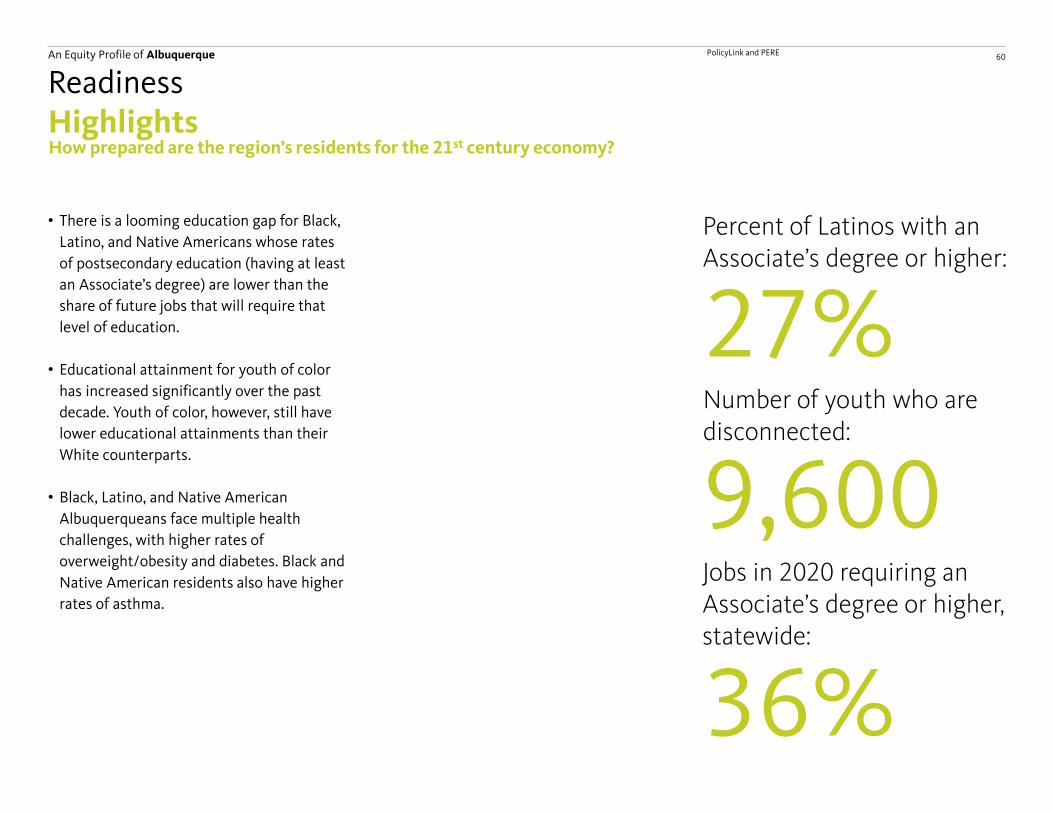
An Equity Profile of Albuquerque PolicyLink and PERE 60
HighlightsReadiness
9,600
How prepared are the region’s residents for the 21st century economy?
Percent of Latinos with an Associate’s degree or higher:
Number of youth who are disconnected:
36%
Jobs in 2020 requiring an Associate’s degree or higher, statewide:
27%
• There is a looming education gap for Black,
Latino, and Native Americans whose rates
of postsecondary education (having at least
an Associate’s degree) are lower than the
share of future jobs that will require that
level of education.
• Educational attainment for youth of color
has increased significantly over the past
decade. Youth of color, however, still have
lower educational attainments than their
White counterparts.
• Black, Latino, and Native American
Albuquerqueans face multiple health
challenges, with higher rates of
overweight/obesity and diabetes. Black and
Native American residents also have higher
rates of asthma.
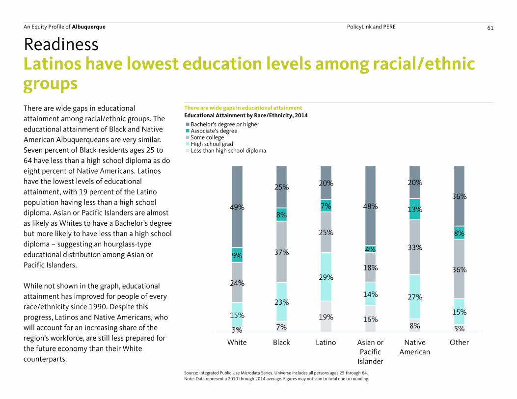
An Equity Profile of Albuquerque PolicyLink and PERE 61
3% 7%
19% 16%8% 5%
15%
23%
29%
14% 27%
15%
24%
37%
25%
18%
33%
36%
9%
8%7%
4%
13%
8%
49%
25%20%
48%
20%
36%
White Black Latino Asian orPacific
Islander
NativeAmerican
Other
Latinos have lowest education levels among racial/ethnic groupsThere are wide gaps in educational
attainment among racial/ethnic groups. The
educational attainment of Black and Native
American Albuquerqueans are very similar.
Seven percent of Black residents ages 25 to
64 have less than a high school diploma as do
eight percent of Native Americans. Latinos
have the lowest levels of educational
attainment, with 19 percent of the Latino
population having less than a high school
diploma. Asian or Pacific Islanders are almost
as likely as Whites to have a Bachelor’s degree
but more likely to have less than a high school
diploma – suggesting an hourglass-type
educational distribution among Asian or
Pacific Islanders.
While not shown in the graph, educational
attainment has improved for people of every
race/ethnicity since 1990. Despite this
progress, Latinos and Native Americans, who
will account for an increasing share of the
region’s workforce, are still less prepared for
the future economy than their White
counterparts.
There are wide gaps in educational attainment
Readiness
Educational Attainment by Race/Ethnicity, 2014
Source: Integrated Public Use Microdata Series. Universe includes all persons ages 25 through 64.
Note: Data represent a 2010 through 2014 average. Figures may not sum to total due to rounding.
3%7%
19%
16%
15%
23%
29%
14%
24%
37%
25%
18%
9%
8%
7%
4%
49%25% 20%
48%
White Black Latino Asian or Pacific Islander
Bachelor's degree or higherAssociate's degreeSome collegeHigh school gradLess than high school diploma
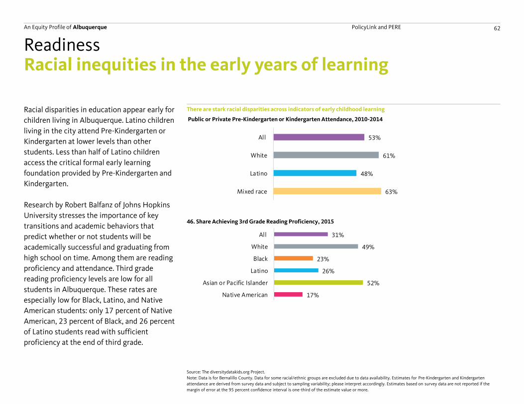
An Equity Profile of Albuquerque PolicyLink and PERE 62
Public or Private Pre-Kindergarten or Kindergarten Attendance, 2010-2014
31%
49%
23%
26%
52%
17%
All
White
Black
Latino
Asian or Pacific Islander
Native American
53%
61%
48%
63%
All
White
Latino
Mixed race
Racial inequities in the early years of learning
Racial disparities in education appear early for
children living in Albuquerque. Latino children
living in the city attend Pre-Kindergarten or
Kindergarten at lower levels than other
students. Less than half of Latino children
access the critical formal early learning
foundation provided by Pre-Kindergarten and
Kindergarten.
Research by Robert Balfanz of Johns Hopkins
University stresses the importance of key
transitions and academic behaviors that
predict whether or not students will be
academically successful and graduating from
high school on time. Among them are reading
proficiency and attendance. Third grade
reading proficiency levels are low for all
students in Albuquerque. These rates are
especially low for Black, Latino, and Native
American students: only 17 percent of Native
American, 23 percent of Black, and 26 percent
of Latino students read with sufficient
proficiency at the end of third grade.
There are stark racial disparities across indicators of early childhood learning
Readiness
Source: The diversitydatakids.org Project.
Note: Data is for Bernalillo County. Data for some racial/ethnic groups are excluded due to data availability. Estimates for Pre-Kindergarten and Kindergarten
attendance are derived from survey data and subject to sampling variability; please interpret accordingly. Estimates based on survey data are not reported if the
margin of error at the 95 percent confidence interval is one-third of the estimate value or more.
46. Share Achieving 3rd Grade Reading Proficiency, 2015
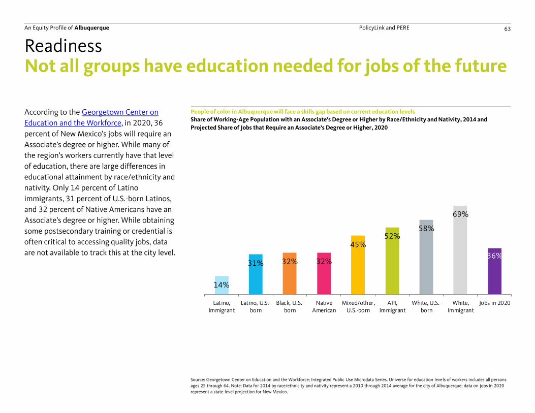
An Equity Profile of Albuquerque PolicyLink and PERE 63
14%
31% 32% 32%
45%52%
58%
69%
36%
Latino,Immigrant
Latino, U.S.-born
Black, U.S.-born
NativeAmerican
Mixed/other,U.S.-born
API,Immigrant
White, U.S.-born
White,Immigrant
Jobs in 2020
Not all groups have education needed for jobs of the future
According to the Georgetown Center on
Education and the Workforce, in 2020, 36
percent of New Mexico’s jobs will require an
Associate’s degree or higher. While many of
the region’s workers currently have that level
of education, there are large differences in
educational attainment by race/ethnicity and
nativity. Only 14 percent of Latino
immigrants, 31 percent of U.S.-born Latinos,
and 32 percent of Native Americans have an
Associate’s degree or higher. While obtaining
some postsecondary training or credential is
often critical to accessing quality jobs, data
are not available to track this at the city level.
People of color in Albuquerque will face a skills gap based on current education levels
Readiness
Share of Working-Age Population with an Associate’s Degree or Higher by Race/Ethnicity and Nativity, 2014 and
Projected Share of Jobs that Require an Associate’s Degree or Higher, 2020
Source: Georgetown Center on Education and the Workforce; Integrated Public Use Microdata Series. Universe for education levels of workers includes all persons
ages 25 through 64. Note: Data for 2014 by race/ethnicity and nativity represent a 2010 through 2014 average for the city of Albuquerque; data on jobs in 2020
represent a state-level projection for New Mexico.
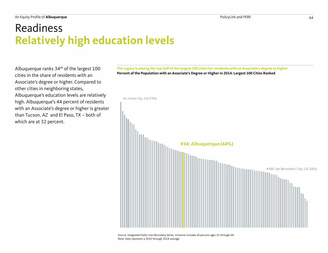
An Equity Profile of Albuquerque PolicyLink and PERE 64
#1: Irvine City, CA (73%)
#34: Albuquerque (44%)
#100: San Bernardino City, CA (16%)
Relatively high education levels
Albuquerque ranks 34th of the largest 100
cities in the share of residents with an
Associate’s degree or higher. Compared to
other cities in neighboring states,
Albuquerque’s education levels are relatively
high. Albuquerque’s 44 percent of residents
with an Associate’s degree or higher is greater
than Tucson, AZ and El Paso, TX – both of
which are at 32 percent.
The region is among the top half of the largest 100 cities for residents with an Associate’s degree or higher
Readiness
Percent of the Population with an Associate’s Degree or Higher in 2014: Largest 100 Cities Ranked
Source: Integrated Public Use Microdata Series. Universe includes all persons ages 25 through 64.
Note: Data represent a 2010 through 2014 average.
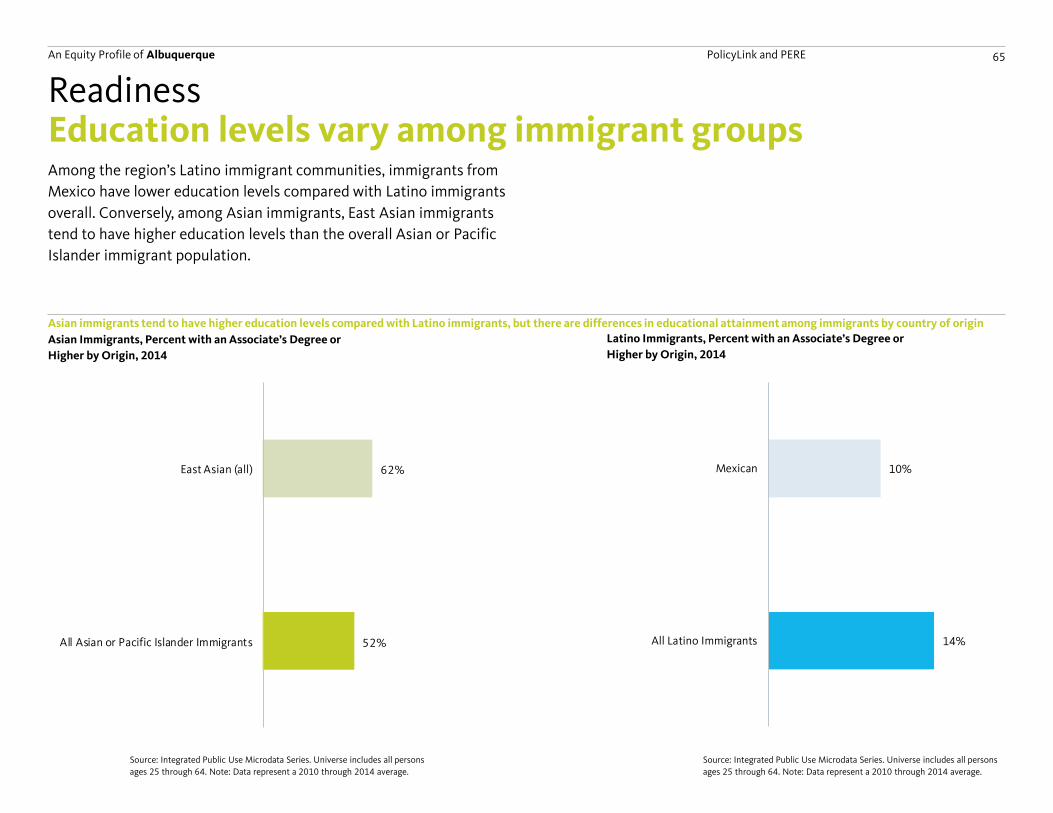
An Equity Profile of Albuquerque PolicyLink and PERE 65
52%
62%
All Asian or Pacific Islander Immigrants
East Asian (all)
14%
10%
All Latino Immigrants
Mexican
Education levels vary among immigrant groups
Asian immigrants tend to have higher education levels compared with Latino immigrants, but there are differences in educational attainment among immigrants by country of origin
Readiness
Asian Immigrants, Percent with an Associate’s Degree or
Higher by Origin, 2014
Source: Integrated Public Use Microdata Series. Universe includes all persons
ages 25 through 64. Note: Data represent a 2010 through 2014 average.
Latino Immigrants, Percent with an Associate’s Degree or
Higher by Origin, 2014
Source: Integrated Public Use Microdata Series. Universe includes all persons
ages 25 through 64. Note: Data represent a 2010 through 2014 average.
Among the region’s Latino immigrant communities, immigrants from
Mexico have lower education levels compared with Latino immigrants
overall. Conversely, among Asian immigrants, East Asian immigrants
tend to have higher education levels than the overall Asian or Pacific
Islander immigrant population.
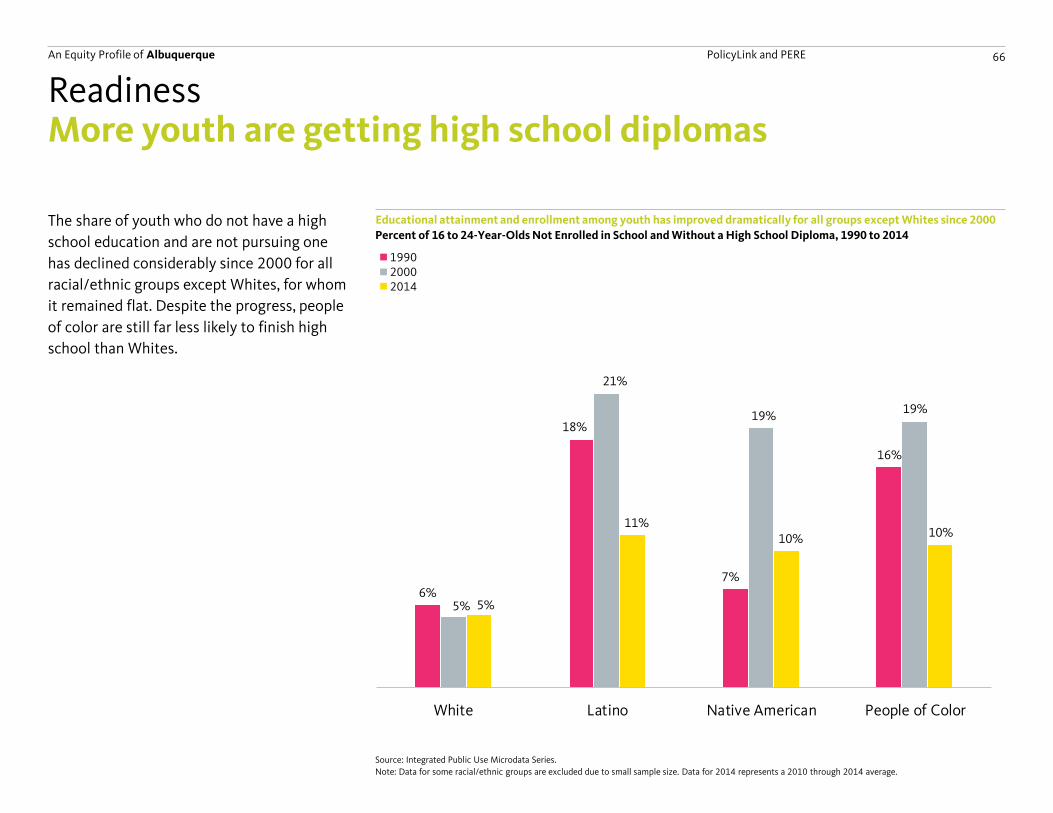
An Equity Profile of Albuquerque PolicyLink and PERE 66
6%
18%
7%
16%
5%
21%
19%19%
5%
11%10% 10%
White Latino Native American People of Color
More youth are getting high school diplomas
The share of youth who do not have a high
school education and are not pursuing one
has declined considerably since 2000 for all
racial/ethnic groups except Whites, for whom
it remained flat. Despite the progress, people
of color are still far less likely to finish high
school than Whites.
Educational attainment and enrollment among youth has improved dramatically for all groups except Whites since 2000
Readiness
Percent of 16 to 24-Year-Olds Not Enrolled in School and Without a High School Diploma, 1990 to 2014
Source: Integrated Public Use Microdata Series.
Note: Data for some racial/ethnic groups are excluded due to small sample size. Data for 2014 represents a 2010 through 2014 average.
11%
20%
0% 0%
11%
16%
54%
0%
3%
15%
23%
0%
White Black Latino API
199020002014
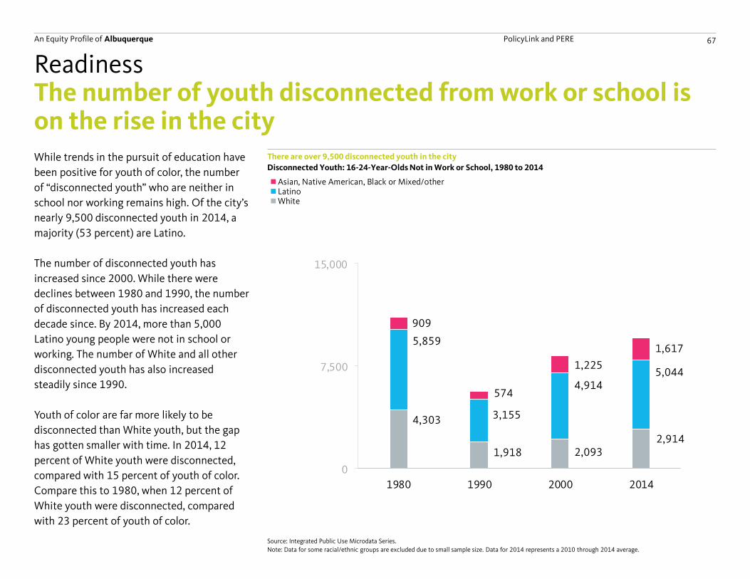
An Equity Profile of Albuquerque PolicyLink and PERE 67
4,303
1,918 2,093 2,914
5,859
3,155
4,914 5,044
909
574
1,225
1,617
0
7,500
15,000
1980 1990 2000 2014
0
20,000
1980 1990 2000 2014
Asian, Native American, Black or Mixed/otherLatinoWhite
The number of youth disconnected from work or school is on the rise in the cityWhile trends in the pursuit of education have
been positive for youth of color, the number
of “disconnected youth” who are neither in
school nor working remains high. Of the city’s
nearly 9,500 disconnected youth in 2014, a
majority (53 percent) are Latino.
The number of disconnected youth has
increased since 2000. While there were
declines between 1980 and 1990, the number
of disconnected youth has increased each
decade since. By 2014, more than 5,000
Latino young people were not in school or
working. The number of White and all other
disconnected youth has also increased
steadily since 1990.
Youth of color are far more likely to be
disconnected than White youth, but the gap
has gotten smaller with time. In 2014, 12
percent of White youth were disconnected,
compared with 15 percent of youth of color.
Compare this to 1980, when 12 percent of
White youth were disconnected, compared
with 23 percent of youth of color.
There are over 9,500 disconnected youth in the city
Readiness
Disconnected Youth: 16-24-Year-Olds Not in Work or School, 1980 to 2014
Source: Integrated Public Use Microdata Series.
Note: Data for some racial/ethnic groups are excluded due to small sample size. Data for 2014 represents a 2010 through 2014 average.
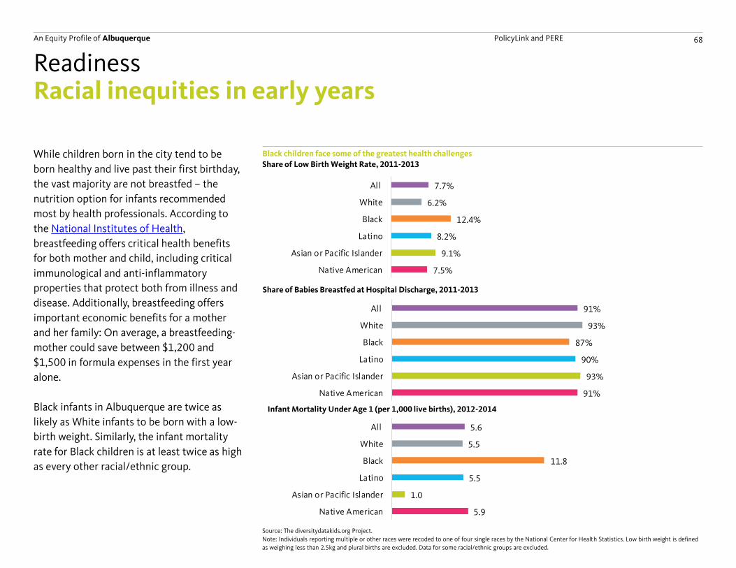
An Equity Profile of Albuquerque PolicyLink and PERE 68
5.6
5.5
11.8
5.5
1.0
5.9
All
White
Black
Latino
Asian or Pacific Islander
Native American
91%
93%
87%
90%
93%
91%
All
White
Black
Latino
Asian or Pacific Islander
Native American
7.7%
6.2%
12.4%
8.2%
9.1%
7.5%
All
White
Black
Latino
Asian or Pacific Islander
Native American
Infant Mortality Under Age 1 (per 1,000 live births), 2012-2014
Racial inequities in early years
While children born in the city tend to be
born healthy and live past their first birthday,
the vast majority are not breastfed – the
nutrition option for infants recommended
most by health professionals. According to
the National Institutes of Health,
breastfeeding offers critical health benefits
for both mother and child, including critical
immunological and anti-inflammatory
properties that protect both from illness and
disease. Additionally, breastfeeding offers
important economic benefits for a mother
and her family: On average, a breastfeeding-
mother could save between $1,200 and
$1,500 in formula expenses in the first year
alone.
Black infants in Albuquerque are twice as
likely as White infants to be born with a low-
birth weight. Similarly, the infant mortality
rate for Black children is at least twice as high
as every other racial/ethnic group.
Black children face some of the greatest health challenges
Readiness
Share of Low Birth Weight Rate, 2011-2013
Source: The diversitydatakids.org Project.
Note: Individuals reporting multiple or other races were recoded to one of four single races by the National Center for Health Statistics. Low birth weight is defined
as weighing less than 2.5kg and plural births are excluded. Data for some racial/ethnic groups are excluded.
Share of Babies Breastfed at Hospital Discharge, 2011-2013
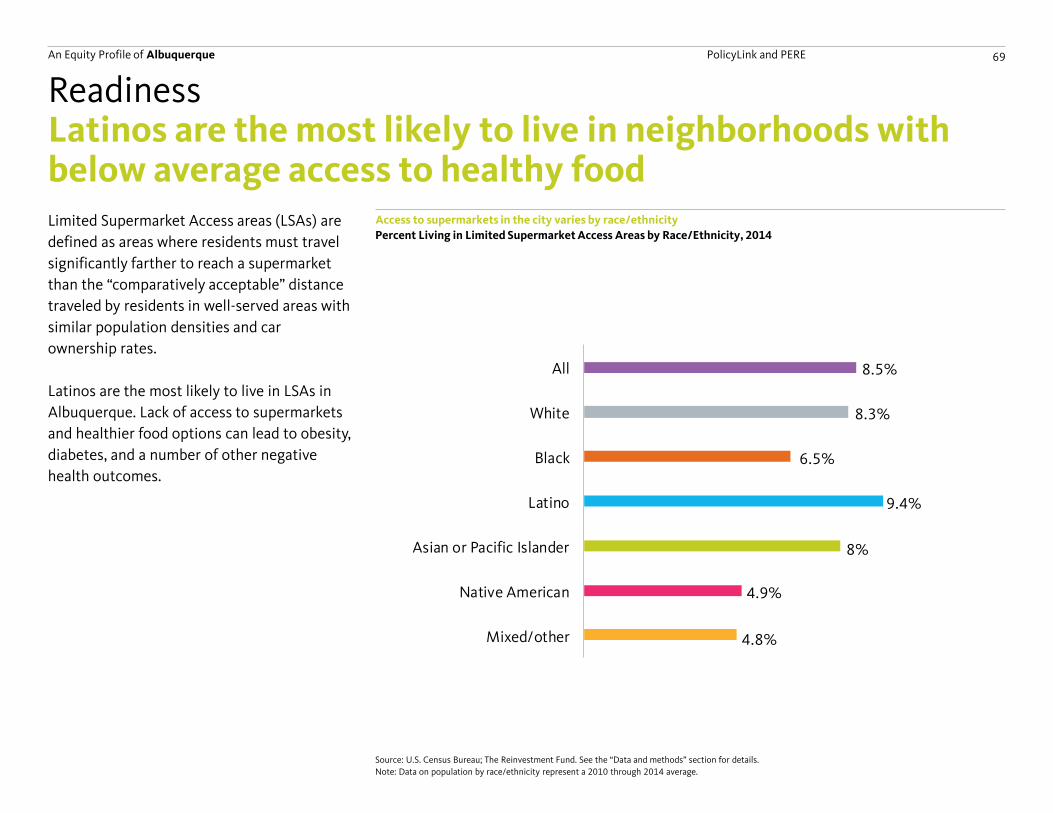
An Equity Profile of Albuquerque PolicyLink and PERE 69
4.8%
4.9%
8%
9.4%
6.5%
8.3%
8.5%
Mixed/other
Native American
Asian or Pacific Islander
Latino
Black
White
All
Latinos are the most likely to live in neighborhoods with below average access to healthy foodLimited Supermarket Access areas (LSAs) are
defined as areas where residents must travel
significantly farther to reach a supermarket
than the “comparatively acceptable” distance
traveled by residents in well-served areas with
similar population densities and car
ownership rates.
Latinos are the most likely to live in LSAs in
Albuquerque. Lack of access to supermarkets
and healthier food options can lead to obesity,
diabetes, and a number of other negative
health outcomes.
Access to supermarkets in the city varies by race/ethnicity
Readiness
Percent Living in Limited Supermarket Access Areas by Race/Ethnicity, 2014
Source: U.S. Census Bureau; The Reinvestment Fund. See the “Data and methods” section for details.
Note: Data on population by race/ethnicity represent a 2010 through 2014 average.
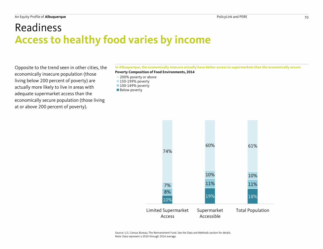
An Equity Profile of Albuquerque PolicyLink and PERE 70
10%19% 18%
8%
11% 11%7%
10% 10%
74%60% 61%
Limited SupermarketAccess
SupermarketAccessible
Total Population
In Albuquerque, the economically insecure actually have better access to supermarkets than the economically secure
Poverty Composition of Food Environments, 2014
30%26% 26%
16%
12% 13%
12%
10% 10%
42% 52% 51…
Limited Food Access Food Accessible Total Population
200% poverty or above150-199% poverty100-149% povertyBelow poverty
Access to healthy food varies by income
Opposite to the trend seen in other cities, the
economically insecure population (those
living below 200 percent of poverty) are
actually more likely to live in areas with
adequate supermarket access than the
economically secure population (those living
at or above 200 percent of poverty).
Readiness
Source: U.S. Census Bureau; The Reinvestment Fund. See the Data and Methods section for details.
Note: Data represent a 2010 through 2014 average.
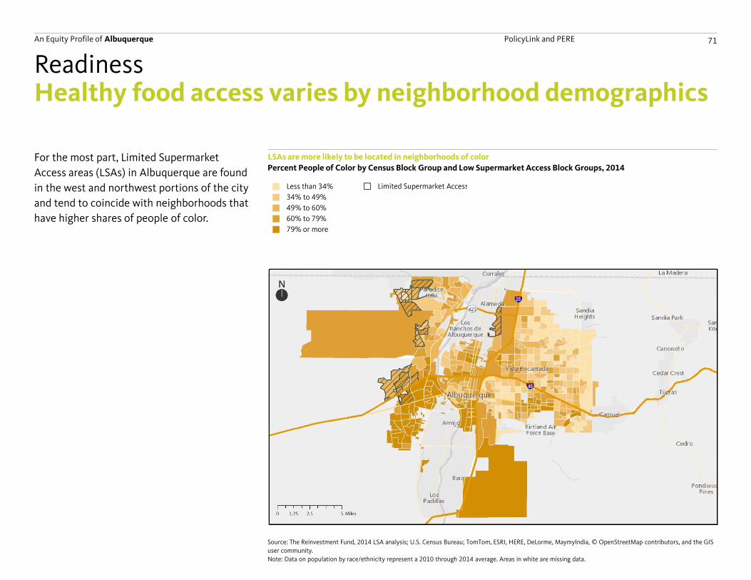
An Equity Profile of Albuquerque PolicyLink and PERE 71
Less than 34%
34% to 49%
49% to 60%
60% to 79%
79% or more
Limited Supermarket Access
Healthy food access varies by neighborhood demographics
For the most part, Limited Supermarket
Access areas (LSAs) in Albuquerque are found
in the west and northwest portions of the city
and tend to coincide with neighborhoods that
have higher shares of people of color.
LSAs are more likely to be located in neighborhoods of color
Readiness
Percent People of Color by Census Block Group and Low Supermarket Access Block Groups, 2014
Source: The Reinvestment Fund, 2014 LSA analysis; U.S. Census Bureau; TomTom, ESRI, HERE, DeLorme, MaymyIndia, © OpenStreetMap contributors, and the GIS
user community.
Note: Data on population by race/ethnicity represent a 2010 through 2014 average. Areas in white are missing data.
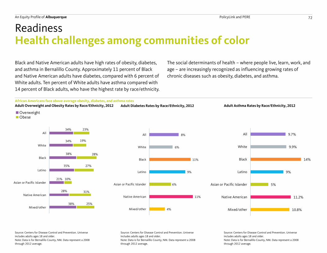
An Equity Profile of Albuquerque PolicyLink and PERE 72
10.8%
11.2%
5%
9%
14%
9.9%
9.7%
Mixed/other
Native American
Asian or Pacific Islander
Latino
Black
White
All
38%
28%
21%
35%
38%
34%
34%
25%
31%
10%
27%
28%
19%
23%
Mixed/other
Native American
Asian or Pacific Islander
Latino
Black
White
All
4%
11%
6%
9%
11%
6%
8%
Mixed/other
Native American
Asian or Pacific Islander
Latino
Black
White
All
Health challenges among communities of color
African Americans face above average obesity, diabetes, and asthma rates
Readiness
Adult Overweight and Obesity Rates by Race/Ethnicity, 2012
Source: Centers for Disease Control and Prevention. Universe
includes adults ages 18 and older.
Note: Data is for Bernalillo County, NM. Data represent a 2008
through 2012 average.
Adult Diabetes Rates by Race/Ethnicity, 2012 Adult Asthma Rates by Race/Ethnicity, 2012
Source: Centers for Disease Control and Prevention. Universe
includes adults ages 18 and older.
Note: Data is for Bernalillo County, NM. Data represent a 2008
through 2012 average.
Source: Centers for Disease Control and Prevention. Universe
includes adults ages 18 and older.
Note: Data is for Bernalillo County, NM. Data represent a 2008
through 2012 average.
Black and Native American adults have high rates of obesity, diabetes,
and asthma in Bernalillo County. Approximately 11 percent of Black
and Native American adults have diabetes, compared with 6 percent of
White adults. Ten percent of White adults have asthma compared with
14 percent of Black adults, who have the highest rate by race/ethnicity.
The social determinants of health – where people live, learn, work, and
age – are increasingly recognized as influencing growing rates of
chronic diseases such as obesity, diabetes, and asthma.
0%
0%
36%
32%
34%
0%
0%
37%
16%
29%
0% 20% 40% 60% 80%
Asian or Pacific Islander
Latino
Black
White
All
OverweightObese
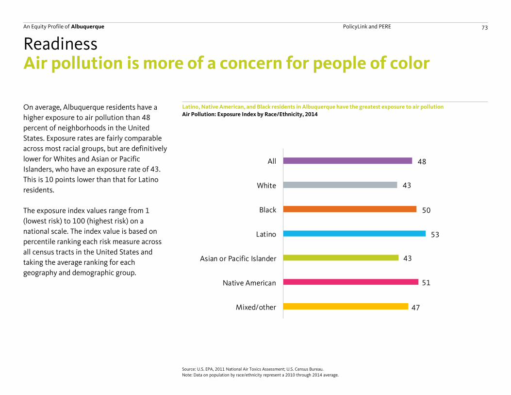
An Equity Profile of Albuquerque PolicyLink and PERE 73
48
43
50
53
43
51
47
All
White
Black
Latino
Asian or Pacific Islander
Native American
Mixed/other
Air pollution is more of a concern for people of color
On average, Albuquerque residents have a
higher exposure to air pollution than 48
percent of neighborhoods in the United
States. Exposure rates are fairly comparable
across most racial groups, but are definitively
lower for Whites and Asian or Pacific
Islanders, who have an exposure rate of 43.
This is 10 points lower than that for Latino
residents.
The exposure index values range from 1
(lowest risk) to 100 (highest risk) on a
national scale. The index value is based on
percentile ranking each risk measure across
all census tracts in the United States and
taking the average ranking for each
geography and demographic group.
Latino, Native American, and Black residents in Albuquerque have the greatest exposure to air pollution
Readiness
Air Pollution: Exposure Index by Race/Ethnicity, 2014
Source: U.S. EPA, 2011 National Air Toxics Assessment; U.S. Census Bureau.
Note: Data on population by race/ethnicity represent a 2010 through 2014 average.
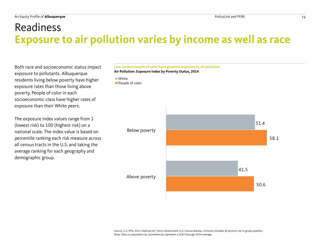
An Equity Profile of Albuquerque PolicyLink and PERE 74
51.4
41.5
58.1
50.6
Below poverty
Above poverty
Exposure to air pollution varies by income as well as race
Both race and socioeconomic status impact
exposure to pollutants. Albuquerque
residents living below poverty have higher
exposure rates than those living above
poverty. People of color in each
socioeconomic class have higher rates of
exposure than their White peers.
The exposure index values range from 1
(lowest risk) to 100 (highest risk) on a
national scale. The index value is based on
percentile ranking each risk measure across
all census tracts in the U.S. and taking the
average ranking for each geography and
demographic group.
Low-income people of color have greatest exposure to air pollution
Readiness
Air Pollution: Exposure Index by Poverty Status, 2014
Source: U.S. EPA, 2011 National Air Toxics Assessment; U.S. Census Bureau. Universe includes all persons not in group quarters.
Note: Data on population by race/ethnicity represent a 2010 through 2014 average.
63.4
57.1
65.7
62.3
Below poverty
Above poverty
WhitePeople of color
An Equity Profile of Albuquerque PolicyLink and PERE 75
Connectedness
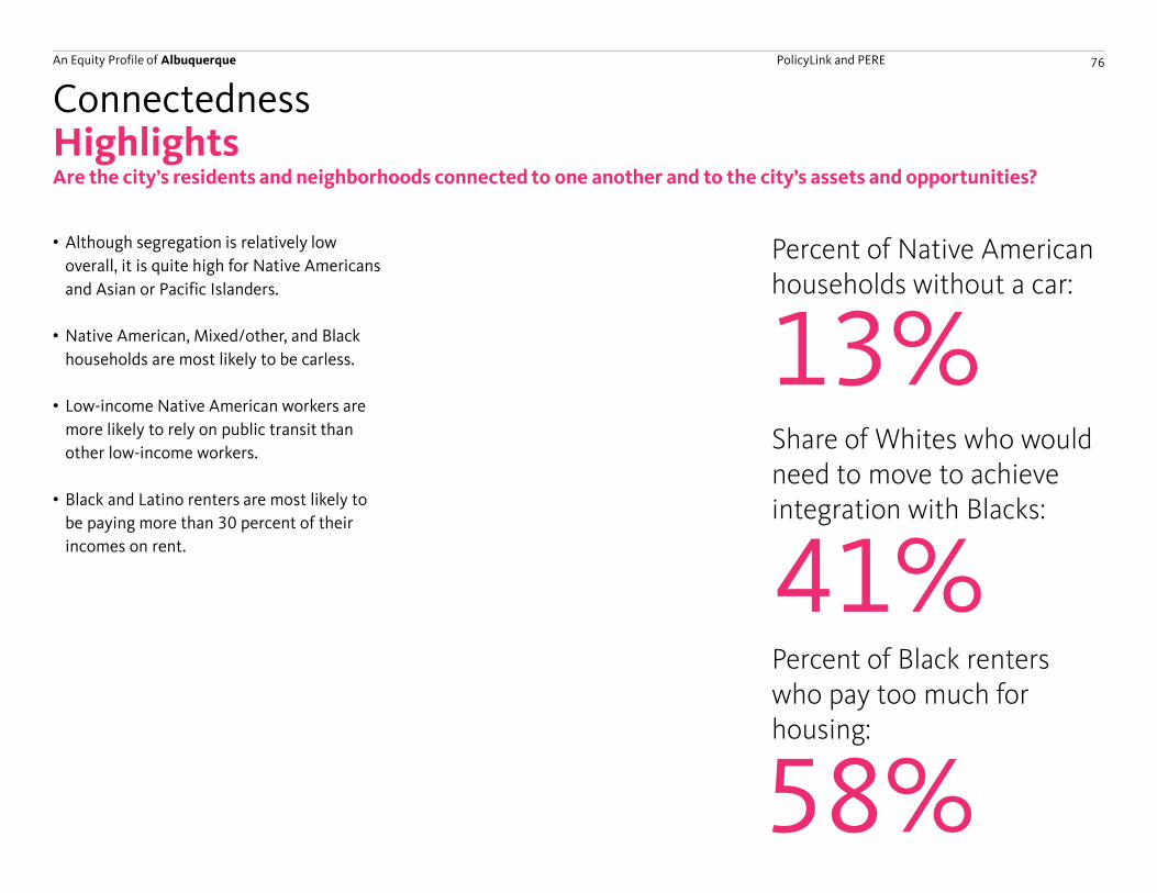
An Equity Profile of Albuquerque PolicyLink and PERE 76
41%
HighlightsConnectedness
Are the city’s residents and neighborhoods connected to one another and to the city’s assets and opportunities?
• Although segregation is relatively low
overall, it is quite high for Native Americans
and Asian or Pacific Islanders.
• Native American, Mixed/other, and Black
households are most likely to be carless.
• Low-income Native American workers are
more likely to rely on public transit than
other low-income workers.
• Black and Latino renters are most likely to
be paying more than 30 percent of their
incomes on rent.
58%
Percent of Black renters who pay too much for housing:
Share of Whites who would need to move to achieve integration with Blacks:
13%Percent of Native American households without a car:
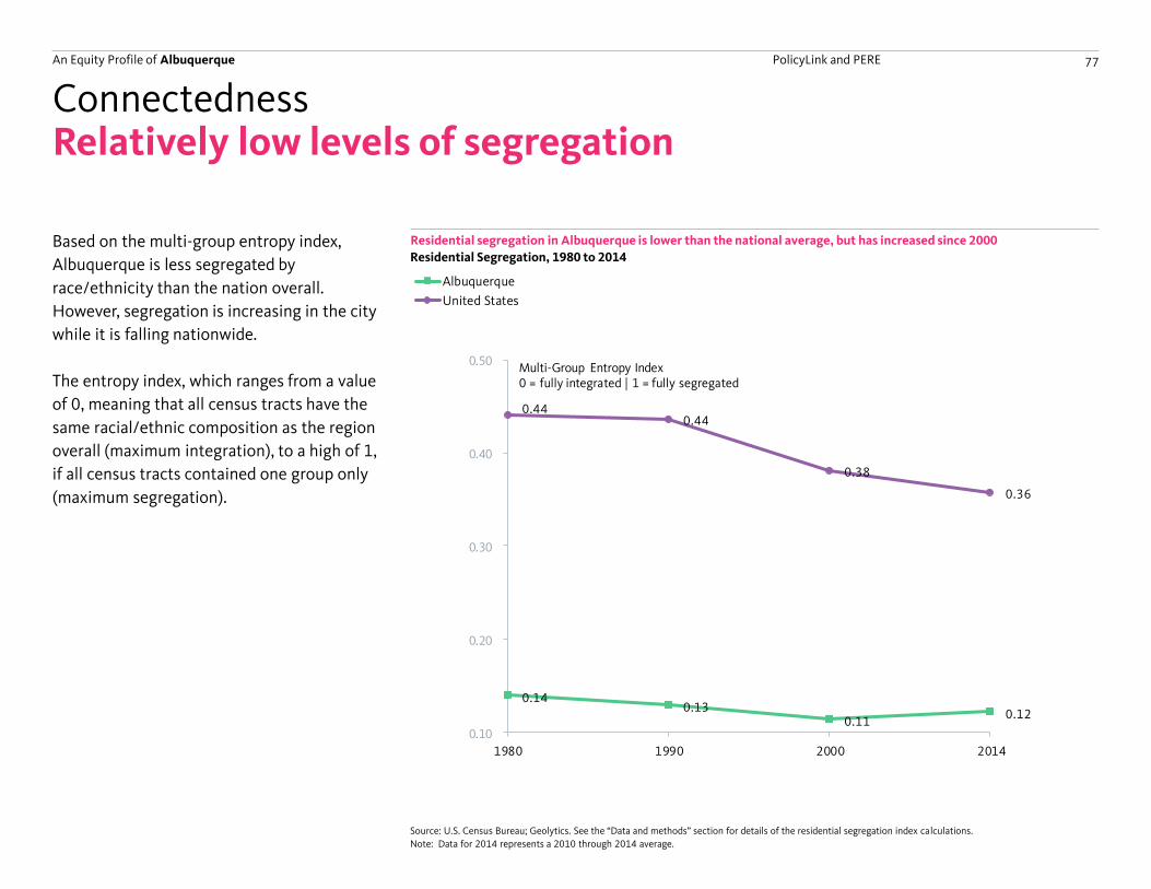
An Equity Profile of Albuquerque PolicyLink and PERE 77
0.14 0.13
0.11 0.12
0.44 0.44
0.38
0.36
0.10
0.20
0.30
0.40
0.50
1980 1990 2000 2014
Multi-Group Entropy Index0 = fully integrated | 1 = fully segregated
Relatively low levels of segregation
Based on the multi-group entropy index,
Albuquerque is less segregated by
race/ethnicity than the nation overall.
However, segregation is increasing in the city
while it is falling nationwide.
The entropy index, which ranges from a value
of 0, meaning that all census tracts have the
same racial/ethnic composition as the region
overall (maximum integration), to a high of 1,
if all census tracts contained one group only
(maximum segregation).
Residential segregation in Albuquerque is lower than the national average, but has increased since 2000
Connectedness
Residential Segregation, 1980 to 2014
Source: U.S. Census Bureau; Geolytics. See the “Data and methods” section for details of the residential segregation index calculations.
Note: Data for 2014 represents a 2010 through 2014 average.
0.44 0.44
0.38
0.36
0.20
0.30
0.40
0.50
1980 1990 2000 2014
Albuquerque
United States
Multi-Group Entropy Index0 = fully integrated | 1 = fully segregated
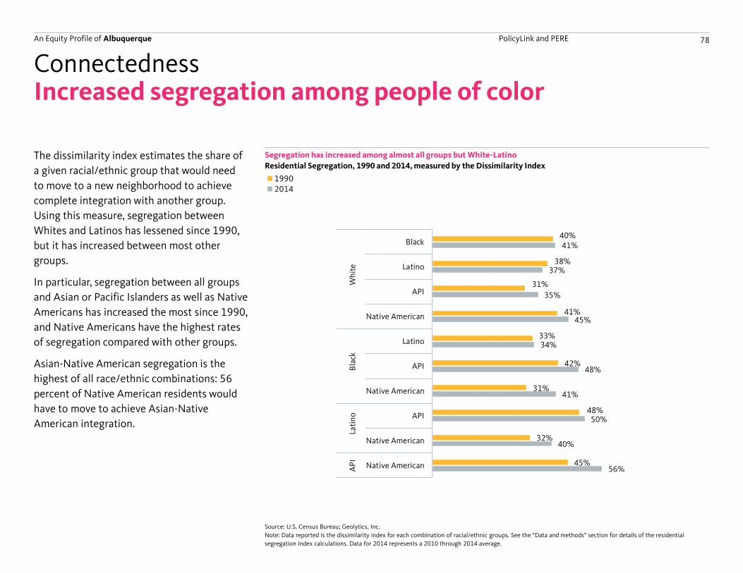
An Equity Profile of Albuquerque PolicyLink and PERE 78
40%
38%
31%
41%
33%
42%
31%
48%
32%
45%
41%
37%
35%
45%
34%
48%
41%
50%
40%
56%
Black
Latino
API
Native American
Latino
API
Native American
API
Native American
Native American
W
hit
e
Bla
ck
Lat
ino
AP
I
63%
50%
41%
49%
59%
56%
69%
50%
48%
55%
48%
53%
48%
58%
47%
60%
68%
65%
64%
67%
Black
Latino
API
Native American
Latino
API
Native American
API
Native American
Native American
W
hit
e
Bla
ck
Lat
ino
AP
I
19902014
Increased segregation among people of color
The dissimilarity index estimates the share of
a given racial/ethnic group that would need
to move to a new neighborhood to achieve
complete integration with another group.
Using this measure, segregation between
Whites and Latinos has lessened since 1990,
but it has increased between most other
groups.
In particular, segregation between all groups
and Asian or Pacific Islanders as well as Native
Americans has increased the most since 1990,
and Native Americans have the highest rates
of segregation compared with other groups.
Asian-Native American segregation is the
highest of all race/ethnic combinations: 56
percent of Native American residents would
have to move to achieve Asian-Native
American integration.
Segregation has increased among almost all groups but White-Latino
Connectedness
Residential Segregation, 1990 and 2014, measured by the Dissimilarity Index
Source: U.S. Census Bureau; Geolytics, Inc.
Note: Data reported is the dissimilarity index for each combination of racial/ethnic groups. See the “Data and methods” section for details of the residential
segregation index calculations. Data for 2014 represents a 2010 through 2014 average.
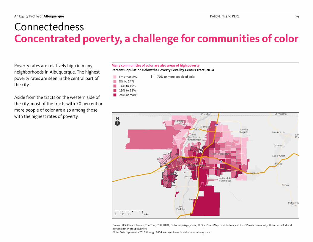
An Equity Profile of Albuquerque PolicyLink and PERE 79
Concentrated poverty, a challenge for communities of color
Poverty rates are relatively high in many
neighborhoods in Albuquerque. The highest
poverty rates are seen in the central part of
the city.
Aside from the tracts on the western side of
the city, most of the tracts with 70 percent or
more people of color are also among those
with the highest rates of poverty.
Many communities of color are also areas of high poverty
Connectedness
Percent Population Below the Poverty Level by Census Tract, 2014
Source: U.S. Census Bureau; TomTom, ESRI, HERE, DeLorme, MaymyIndia, © OpenStreetMap contributors, and the GIS user community. Universe includes all
persons not in group quarters.
Note: Data represent a 2010 through 2014 average. Areas in white have missing data.
8% to 14%
14% to 19%
19% to 28%
28% or more
Less than 8% 70% or more people of color
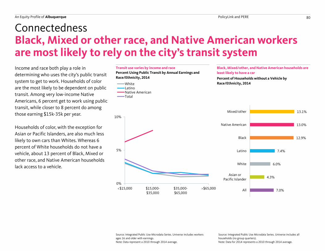
An Equity Profile of Albuquerque PolicyLink and PERE 80
7.0%
4.3%
6.0%
7.4%
12.9%
13.0%
13.1%
All
Asian orPacific Islander
White
Latino
Black
Native American
Mixed/other
0%
5%
10%
<$15,000 $15,000-$35,000
$35,000-$65,000
>$65,000
Black, Mixed or other race, and Native American workers are most likely to rely on the city’s transit systemIncome and race both play a role in
determining who uses the city’s public transit
system to get to work. Households of color
are the most likely to be dependent on public
transit. Among very low-income Native
Americans, 6 percent get to work using public
transit, while closer to 8 percent do among
those earning $15k-35k per year.
Households of color, with the exception for
Asian or Pacific Islanders, are also much less
likely to own cars than Whites. Whereas 6
percent of White households do not have a
vehicle, about 13 percent of Black, Mixed or
other race, and Native American households
lack access to a vehicle.
Transit use varies by income and race
Connectedness
Percent Using Public Transit by Annual Earnings and
Race/Ethnicity, 2014
Source: Integrated Public Use Microdata Series. Universe includes workers
ages 16 and older with earnings.
Note: Data represent a 2010 through 2014 average.
Black, Mixed/other, and Native American households are
least likely to have a car
Percent of Households without a Vehicle by
Race/Ethnicity, 2014
Source: Integrated Public Use Microdata Series. Universe includes all
households (no group quarters).
Note: Data for 2014 represents a 2010 through 2014 average.
0%
1%
2%
3%
4%
5%
6%
7%
8%
9%
<$15,000 $15,000-$35,000
$35,000-$65,000
>$65,000
WhiteLatinoNative AmericanTotal
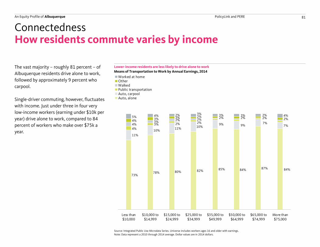
An Equity Profile of Albuquerque PolicyLink and PERE 81
73%78% 80% 82% 85% 84% 87% 84%
11%
10%11%
10%9% 9%
7%7%
4%
3% 2% 2%4%3% 2% 2%4%3% 3% 2% 2% 2% 2% 2%
5% 4% 2% 3% 3% 3% 2% 4%
Less than$10,000
$10,000 to$14,999
$15,000 to$24,999
$25,000 to$34,999
$35,000 to$49,999
$50,000 to$64,999
$65,000 to$74,999
More than$75,000
73%78%
80%82%
85% 84% 87% 84%11%
10% 11% 10% 9% 9% 7%7%
4%3% 2%
2%1% 1% 1%
1%4%3% 3% 2% 2%
5% 4% 2% 3% 3% 3% 2% 4%
Less than $10,000 $10,000 to $14,999 $15,000 to $24,999 $25,000 to $34,999 $35,000 to $49,999 $50,000 to $64,999 $65,000 to $74,999 More than $75,000
Worked at homeOtherWalkedPublic transportationAuto, carpoolAuto, alone
How residents commute varies by income
The vast majority – roughly 81 percent – of
Albuquerque residents drive alone to work,
followed by approximately 9 percent who
carpool.
Single-driver commuting, however, fluctuates
with income. Just under three in four very
low-income workers (earning under $10k per
year) drive alone to work, compared to 84
percent of workers who make over $75k a
year.
Lower-income residents are less likely to drive alone to work
Connectedness
Means of Transportation to Work by Annual Earnings, 2014
Source: Integrated Public Use Microdata Series. Universe includes workers ages 16 and older with earnings.
Note: Data represent a 2010 through 2014 average. Dollar values are in 2014 dollars.
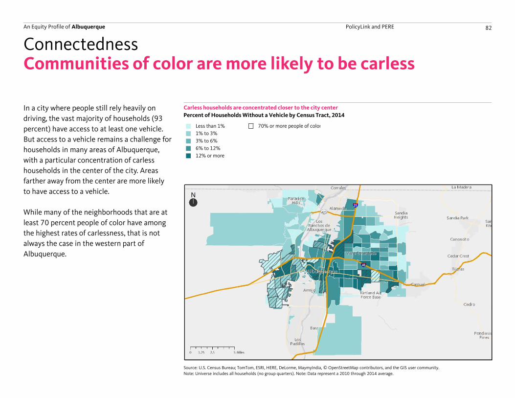
An Equity Profile of Albuquerque PolicyLink and PERE 82
Communities of color are more likely to be carless
In a city where people still rely heavily on
driving, the vast majority of households (93
percent) have access to at least one vehicle.
But access to a vehicle remains a challenge for
households in many areas of Albuquerque,
with a particular concentration of carless
households in the center of the city. Areas
farther away from the center are more likely
to have access to a vehicle.
While many of the neighborhoods that are at
least 70 percent people of color have among
the highest rates of carlessness, that is not
always the case in the western part of
Albuquerque.
Carless households are concentrated closer to the city center
Connectedness
Percent of Households Without a Vehicle by Census Tract, 2014
Source: U.S. Census Bureau; TomTom, ESRI, HERE, DeLorme, MaymyIndia, © OpenStreetMap contributors, and the GIS user community.
Note: Universe includes all households (no group quarters). Note: Data represent a 2010 through 2014 average.
Less than 1%
1% to 3%
3% to 6%
6% to 12%
12% or more
70% or more people of color
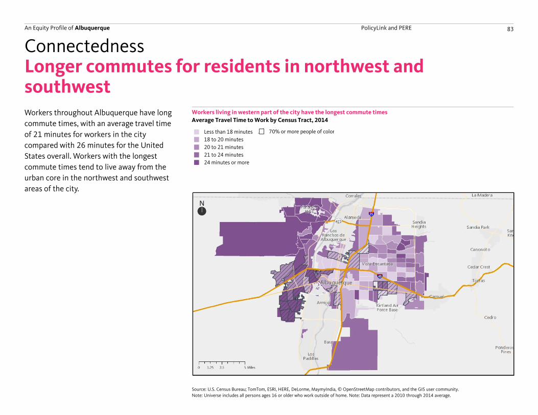
An Equity Profile of Albuquerque PolicyLink and PERE 83
Longer commutes for residents in northwest and southwestWorkers throughout Albuquerque have long
commute times, with an average travel time
of 21 minutes for workers in the city
compared with 26 minutes for the United
States overall. Workers with the longest
commute times tend to live away from the
urban core in the northwest and southwest
areas of the city.
Workers living in western part of the city have the longest commute times
Connectedness
Average Travel Time to Work by Census Tract, 2014
Source: U.S. Census Bureau; TomTom, ESRI, HERE, DeLorme, MaymyIndia, © OpenStreetMap contributors, and the GIS user community.
Note: Universe includes all persons ages 16 or older who work outside of home. Note: Data represent a 2010 through 2014 average.
Less than 18 minutes
18 to 20 minutes
20 to 21 minutes
21 to 24 minutes
24 minutes or more
70% or more people of color
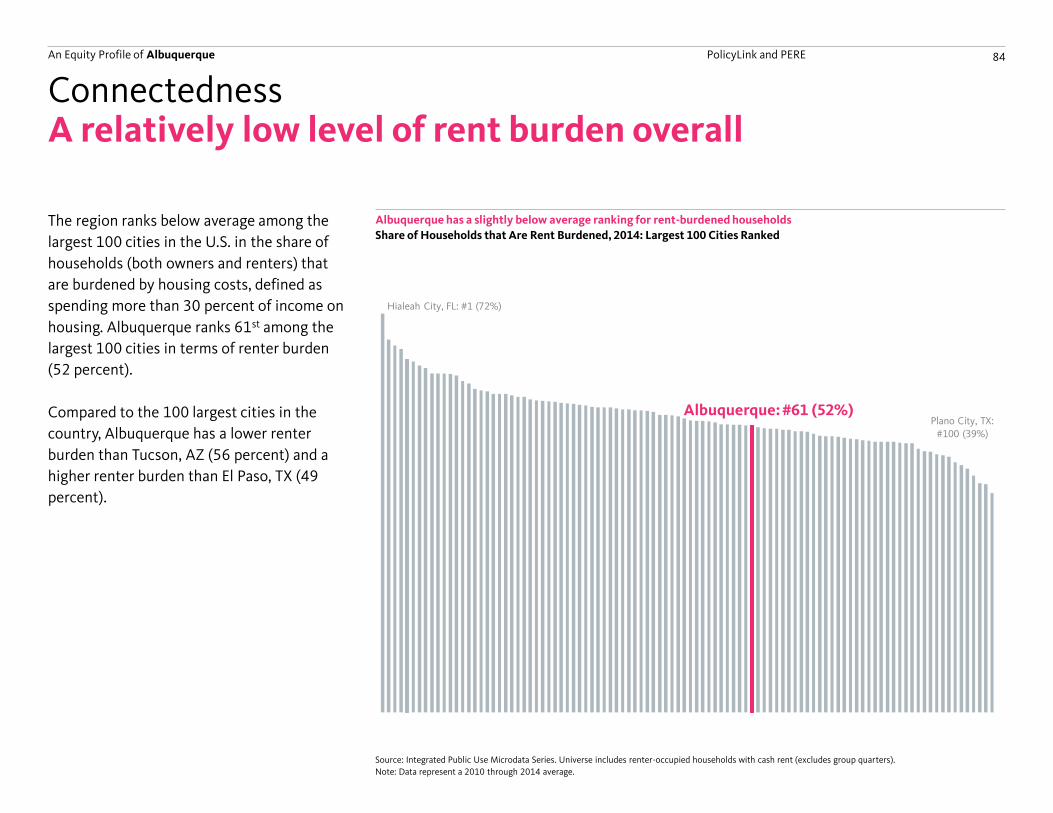
An Equity Profile of Albuquerque PolicyLink and PERE 84
Hialeah City, FL: #1 (72%)
Albuquerque: #61 (52%)Plano City, TX:
#100 (39%)
A relatively low level of rent burden overall
The region ranks below average among the
largest 100 cities in the U.S. in the share of
households (both owners and renters) that
are burdened by housing costs, defined as
spending more than 30 percent of income on
housing. Albuquerque ranks 61st among the
largest 100 cities in terms of renter burden
(52 percent).
Compared to the 100 largest cities in the
country, Albuquerque has a lower renter
burden than Tucson, AZ (56 percent) and a
higher renter burden than El Paso, TX (49
percent).
Albuquerque has a slightly below average ranking for rent-burdened households
Connectedness
Share of Households that Are Rent Burdened, 2014: Largest 100 Cities Ranked
Source: Integrated Public Use Microdata Series. Universe includes renter-occupied households with cash rent (excludes group quarters).
Note: Data represent a 2010 through 2014 average.
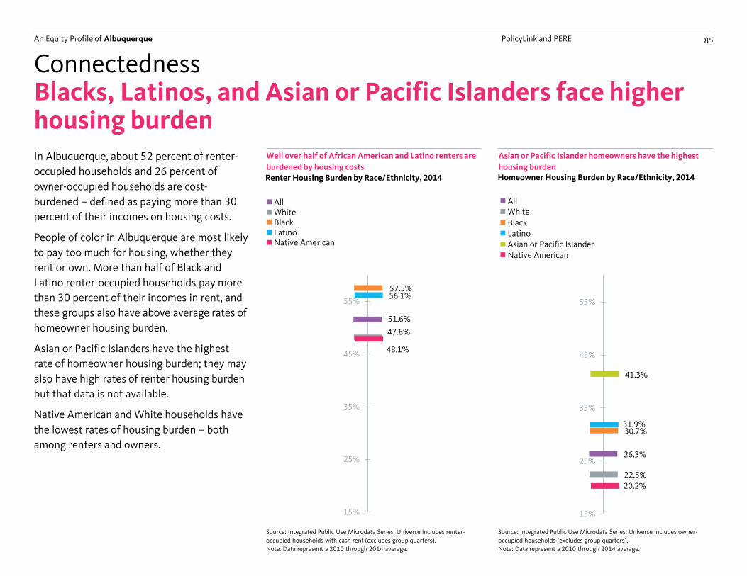
An Equity Profile of Albuquerque PolicyLink and PERE 85
51.6%
48.1%
57.5%56.1%
47.8%
15%
25%
35%
45%
55%
26.3%
22.5%
30.7%31.9%
41.3%
20.2%
15%
25%
35%
45%
55%
26.3%
22.5%
30.7%31.9%
41.3%
20.2%
15%
20%
25%
30%
35%
40%
45%
AllWhiteBlackLatinoAsian or Pacific IslanderNative American
51.6%
48.1%
57.5%56.1%
47.8%
45%
47%
49%
51%
53%
55%
57%
59%
AllWhiteBlackLatinoNative American
Blacks, Latinos, and Asian or Pacific Islanders face higher housing burdenIn Albuquerque, about 52 percent of renter-
occupied households and 26 percent of
owner-occupied households are cost-
burdened – defined as paying more than 30
percent of their incomes on housing costs.
People of color in Albuquerque are most likely
to pay too much for housing, whether they
rent or own. More than half of Black and
Latino renter-occupied households pay more
than 30 percent of their incomes in rent, and
these groups also have above average rates of
homeowner housing burden.
Asian or Pacific Islanders have the highest
rate of homeowner housing burden; they may
also have high rates of renter housing burden
but that data is not available.
Native American and White households have
the lowest rates of housing burden – both
among renters and owners.
Well over half of African American and Latino renters are
burdened by housing costs
Connectedness
Renter Housing Burden by Race/Ethnicity, 2014
Source: Integrated Public Use Microdata Series. Universe includes owner-
occupied households (excludes group quarters).
Note: Data represent a 2010 through 2014 average.
Source: Integrated Public Use Microdata Series. Universe includes renter-
occupied households with cash rent (excludes group quarters).
Note: Data represent a 2010 through 2014 average.
Homeowner Housing Burden by Race/Ethnicity, 2014
Asian or Pacific Islander homeowners have the highest
housing burden
An Equity Profile of Albuquerque PolicyLink and PERE 86
Economic benefits
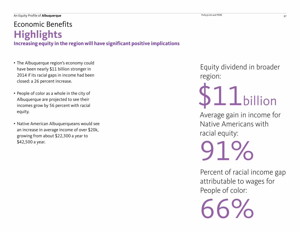
An Equity Profile of Albuquerque PolicyLink and PERE 87
Highlights
Average gain in income for Native Americans with racial equity:
Economic Benefits
Equity dividend in broader region:
Percent of racial income gap attributable to wages for People of color:
91%
$11billion
66%
Increasing equity in the region will have significant positive implications
• The Albuquerque region’s economy could
have been nearly $11 billion stronger in
2014 if its racial gaps in income had been
closed: a 26 percent increase.
• People of color as a whole in the city of
Albuquerque are projected to see their
incomes grow by 56 percent with racial
equity.
• Native American Albuquerqueans would see
an increase in average income of over $20k,
growing from about $22,300 a year to
$42,500 a year.
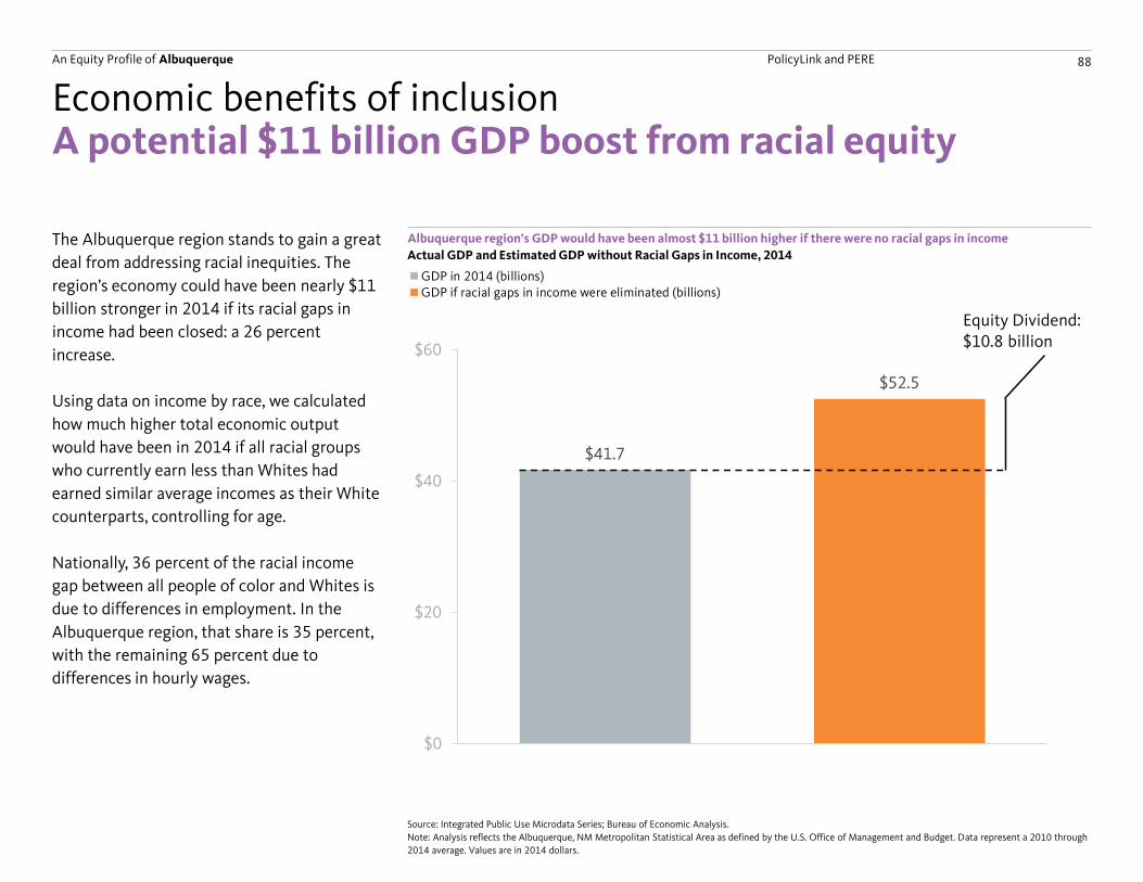
An Equity Profile of Albuquerque PolicyLink and PERE 88
$41.7
$52.5
$0
$20
$40
$60
Equity Dividend: $10.8 billion
A potential $11 billion GDP boost from racial equity
The Albuquerque region stands to gain a great
deal from addressing racial inequities. The
region’s economy could have been nearly $11
billion stronger in 2014 if its racial gaps in
income had been closed: a 26 percent
increase.
Using data on income by race, we calculated
how much higher total economic output
would have been in 2014 if all racial groups
who currently earn less than Whites had
earned similar average incomes as their White
counterparts, controlling for age.
Nationally, 36 percent of the racial income
gap between all people of color and Whites is
due to differences in employment. In the
Albuquerque region, that share is 35 percent,
with the remaining 65 percent due to
differences in hourly wages.
Albuquerque region’s GDP would have been almost $11 billion higher if there were no racial gaps in income
Economic benefits of inclusion
Actual GDP and Estimated GDP without Racial Gaps in Income, 2014
Source: Integrated Public Use Microdata Series; Bureau of Economic Analysis.
Note: Analysis reflects the Albuquerque, NM Metropolitan Statistical Area as defined by the U.S. Office of Management and Budget. Data represent a 2010 through
2014 average. Values are in 2014 dollars.
$41.3
$45.3
$0
$5
$10
$15
$20
$25
$30
$35
$40
$45
$50
GDP in 2014 (billions)GDP if racial gaps in income were eliminated (billions)
Equity Dividend: $4.0 billion
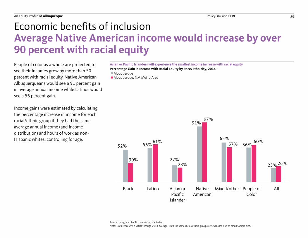
An Equity Profile of Albuquerque PolicyLink and PERE 89
52%56%
27%
91%
65%
56%
30%
61%
23%
97%
57%60%
Black Latino Asian or PacificIslander
Native American Mixed/other People of Color
AlbuquerqueAlbuquerque, NM Metro Area
52% 56%
27%
91%
65%
56%
23%30%
61%
23%
97%
57%60%
26%
Black Latino Asian orPacific
Islander
NativeAmerican
Mixed/other People ofColor
All
People of color as a whole are projected to
see their incomes grow by more than 50
percent with racial equity. Native American
Albuquerqueans would see a 91 percent gain
in average annual income while Latinos would
see a 56 percent gain.
Income gains were estimated by calculating
the percentage increase in income for each
racial/ethnic group if they had the same
average annual income (and income
distribution) and hours of work as non-
Hispanic whites, controlling for age.
Asian or Pacific Islanders will experience the smallest income increase with racial equity
Economic benefits of inclusion
Percentage Gain in Income with Racial Equity by Race/Ethnicity, 2014
Source: Integrated Public Use Microdata Series.
Note: Data represent a 2010 through 2014 average. Data for some racial/ethnic groups are excluded due to small sample size.
Average Native American income would increase by over 90 percent with racial equity
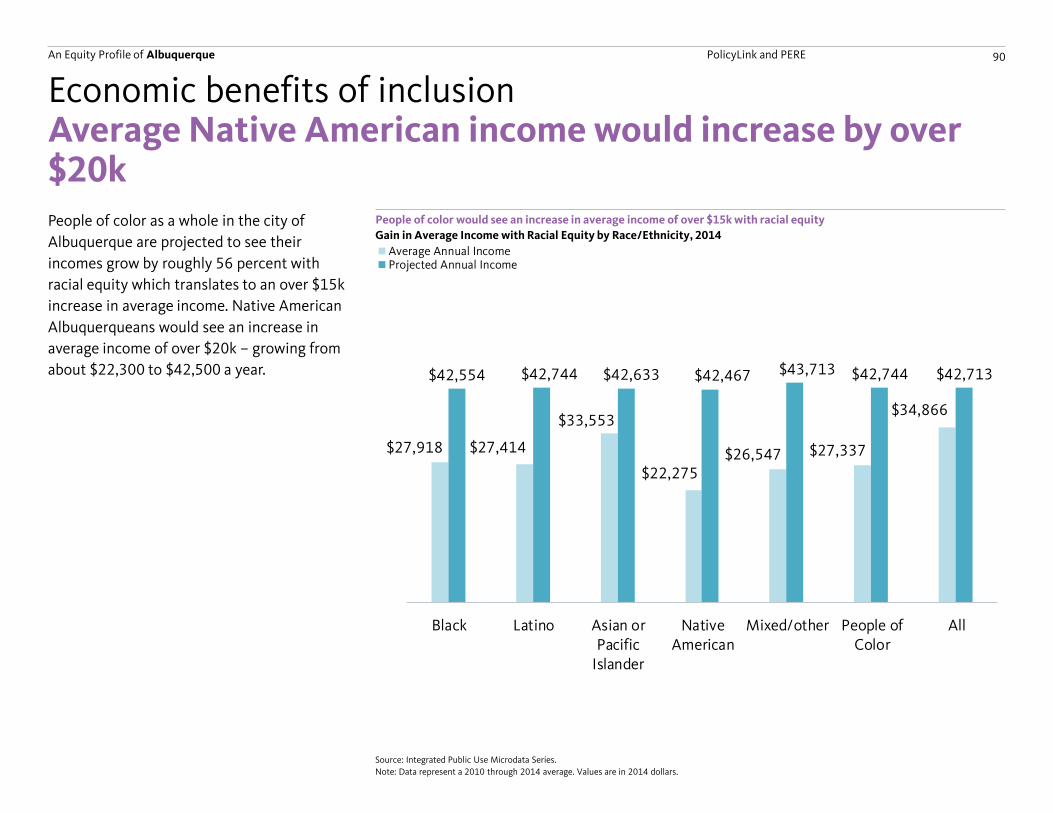
An Equity Profile of Albuquerque PolicyLink and PERE 90
$27,918 $27,414
$33,553
$22,275$26,547 $27,337
$34,866
$42,554 $42,744 $42,633 $42,467 $43,713 $42,744 $42,713
Black Latino Asian orPacific
Islander
NativeAmerican
Mixed/other People ofColor
All
Average Native American income would increase by over $20kPeople of color as a whole in the city of
Albuquerque are projected to see their
incomes grow by roughly 56 percent with
racial equity which translates to an over $15k
increase in average income. Native American
Albuquerqueans would see an increase in
average income of over $20k – growing from
about $22,300 to $42,500 a year.
People of color would see an increase in average income of over $15k with racial equity
Economic benefits of inclusion
Gain in Average Income with Racial Equity by Race/Ethnicity, 2014
Source: Integrated Public Use Microdata Series.
Note: Data represent a 2010 through 2014 average. Values are in 2014 dollars.
$16,550 $17,195
$20,866
$-
$17,445 $17,176
$26,303
$31,271 $30,857 $31,879
$-
$31,452 $31,157 $31,254
Black Latino Asian orPacific
Islander
NativeAmerican
Mixed/other People ofColor
All
Average Annual IncomeProjected Annual Income
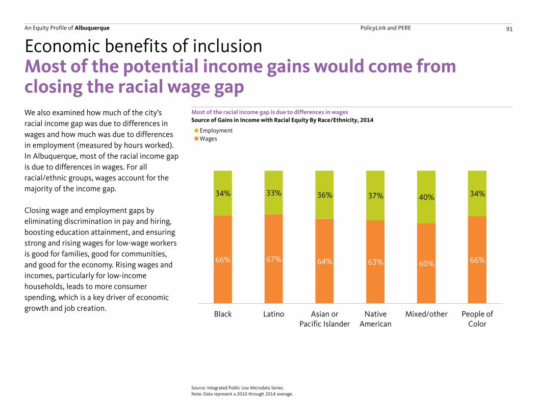
An Equity Profile of Albuquerque PolicyLink and PERE 91
66% 67% 64% 63% 60% 66%
34% 33% 36% 37% 40% 34%
Black Latino Asian orPacific Islander
NativeAmerican
Mixed/other People ofColor
22%
79%
23%
40%31%
78%
40%
21%
77%
60%69%
Black Latino Asian or PacificIslander
Mixed/other People of Color All
Employment
Wages
Most of the potential income gains would come from closing the racial wage gapWe also examined how much of the city’s
racial income gap was due to differences in
wages and how much was due to differences
in employment (measured by hours worked).
In Albuquerque, most of the racial income gap
is due to differences in wages. For all
racial/ethnic groups, wages account for the
majority of the income gap.
Closing wage and employment gaps by
eliminating discrimination in pay and hiring,
boosting education attainment, and ensuring
strong and rising wages for low-wage workers
is good for families, good for communities,
and good for the economy. Rising wages and
incomes, particularly for low-income
households, leads to more consumer
spending, which is a key driver of economic
growth and job creation.
Most of the racial income gap is due to differences in wages
Economic benefits of inclusion
Source of Gains in Income with Racial Equity By Race/Ethnicity, 2014
Source: Integrated Public Use Microdata Series.
Note: Data represent a 2010 through 2014 average.
An Equity Profile of Albuquerque PolicyLink and PERE 92
Implications
An Equity Profile of Albuquerque PolicyLink and PERE 93
Albuquerque’s growing, diverse population is a major economic asset that will help the city compete in the global economy, if the city’s leaders invest in ensuring all of its residents can connect to good jobs and contribute their talent and creativity to building a strong next economy. Business, community, and political leaders must work together to connect communities of color to jobs, business opportunities, quality education and career training. Tremendous work is already underway, which can be strengthened and built upon. PolicyLink and PERE suggest the following areas of focus to ensure all residents – particularly low-income residents and communities of color – contribute to and benefit from the region’s vibrant, equitable economic future.
Grow good jobsJob growth in the Bernalillo County is significantly higher than the nation overall, and the Gross Regional Product remains higher than the national average. However, job growth is not keeping up with population growth and unemployment among people of color in the city is higher than the national average. Albuquerque needs to create a significant number of new, well-paying jobs –
Implications
and ensure that the city’s labor force (particularly women and youth of color) are connected to those jobs. This entails a two-pronged approach. First, economic and workforce development efforts should focus on entrepreneurship and business development in industries that are growing and tend to pay good wages such as construction and life, physical, and social science technicians.
Second, the jobs that are being created need to be good jobs. Wages have declined more than 10 percent for Albuquerque’s lowest income workers since 1979, and the rate of working poverty has been increasing, particularly for workers of color. Advocates and policymakers should consider efforts that will raise wages and provide important worker benefits, such as those outlined by Family Friendly New Mexico.
Connect unemployed and low-wage workers to careers in high-growth industriesIn tandem with job creation efforts, it is vital for Albuquerque to connect its workforce with jobs that pay good wages and offer career opportunities. Communities of color face the
highest unemployment and higher rates of
poverty than their White peers. Our analysis
of strong industries and high-opportunity
occupations reinforces the importance of
current workforce training. Partnerships
between employers and workforce agencies
have proven track records connecting workers
to good careers. In addition, leverage the
economic power of large anchor institutions,
like hospitals and universities. These anchors
can develop intentional strategies to hire
jobseekers facing barriers to employment,
create on-the-job training opportunities, and
purchase more goods and services from local-
and minority-owned businesses who provide
local jobs.
Strengthen educational pathways
Educational attainment for Latino, Black, and
Native American residents is a critical issue
for the long-term economic strength of the
city. While 36 percent of all jobs in New
Mexico by 2020 will require an Associate’s
degree or higher, less than one third of
residents in these groups have attained that
level of
Advancing equity and racial inclusion
An Equity Profile of Albuquerque PolicyLink and PERE 94
education or higher. The city’s rate of
disconnected youth – those not in school or
working – should be prioritized. Scholarships
for programs leading to a postsecondary
vocational certificate or Associate’s degree
can reduce financial barriers to higher
education and can encourage high school
students to stay connected to school,
addressing the high rate of disconnected
youth in the city. Programs like these should
be strengthened and expanded to increase
graduation rates for high school, Associate’s
degrees, and vocational certification
programs throughout the city. Educational
supports should begin even earlier, with
middle-school and high-school curricula that
introduce important 21st century skills, like
coding and app and website development.
Build communities of opportunity throughout the cityAll neighborhoods located throughout the
city should provide their residents with the
ingredients they need to thrive and also open
Implications
up opportunities for low-income residents
and people of color to live in neighborhoods
that are already rich with opportunity (and
from which they’ve historically been
excluded).
Coordinating transportation, housing, and
economic development investments over the
long term will foster more equitable
development patterns and healthier
neighborhoods across the city. Policymakers
should align planning efforts and resources to
promote more affordable transit oriented
development, which is both environmentally
sustainable and a useful vehicle for linking
residents to economic opportunity.
Addressing lingering racially discriminatory
housing and lending practices, and enforcing
fair housing laws, are also critical to expand
opportunity for all.
ConclusionCommunity leaders in the public, private, and nonprofit sectors are already taking steps to connect its more vulnerable communities to educational and economic opportunities, and these efforts must continue. To secure a prosperous future, Albuquerque needs to implement a growth model that is driven by equity –just and fair inclusion into a society in which everyone can participate and prosper. Concerted investments and policies for, and developed from within, communities of color will also be essential to ensure the city’s fastest-growing populations are ready to lead it into the next economy.
Advancing equity and racial inclusion(continued)
PolicyLink and PEREAn Equity Profile of Albuquerque
Data source summary and regional geography
Adjustments made to census summary data on race/ethnicity by age
Adjustments made to demographic projections
95
Data and methods
Broad racial/ethnic origin
Detailed racial/ethnic ancestry
Other selected terms
Selected terms and general notes
Nativity
General notes on analyses
Summary measures from IPUMS microdata
Adjustments at the state and national levels
Estimates and adjustments made to BEA data on GDP
County and metropolitan area estimates
Middle-class analysis
Assembling a complete dataset on employment and wagesby industry
Growth in jobs and earnings by industry wage level, 1990 to 2015
Analysis of occupations by opportunity level
Health data and analysis
Analysis of access to healthy food
Air pollution data and analysis
Measures of diversity and segregation
National projections
County and regional projections
Estimates of GDP without racial gaps in income
103
96
103
97
97
97
98
97
98
101
99
103
105
107
105
105
108
109
110
112
113
114
115
116
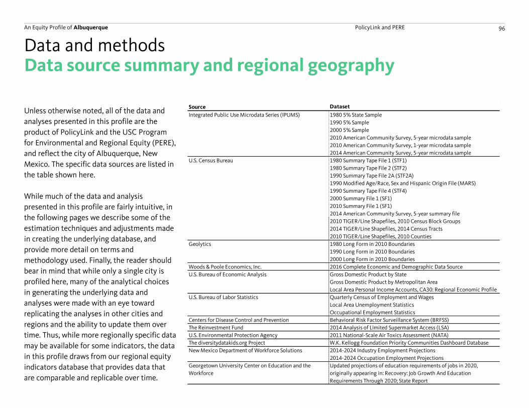
An Equity Profile of Albuquerque PolicyLink and PERE 96
Source Dataset
Integrated Public Use Microdata Series (IPUMS) 1980 5% State Sample
1990 5% Sample
2000 5% Sample
2010 American Community Survey, 5-year microdata sample
2010 American Community Survey, 1-year microdata sample
2014 American Community Survey, 5-year microdata sample
U.S. Census Bureau 1980 Summary Tape File 1 (STF1)
1980 Summary Tape File 2 (STF2)
1990 Summary Tape File 2A (STF2A)
1990 Modified Age/Race, Sex and Hispanic Origin File (MARS)
1990 Summary Tape File 4 (STF4)
2000 Summary File 1 (SF1)
2010 Summary File 1 (SF1)
2014 American Community Survey, 5-year summary file
2010 TIGER/Line Shapefiles, 2010 Census Block Groups
2014 TIGER/Line Shapefiles, 2014 Census Tracts
2010 TIGER/Line Shapefiles, 2010 Counties
Geolytics 1980 Long Form in 2010 Boundaries
1990 Long Form in 2010 Boundaries
2000 Long Form in 2010 Boundaries
Woods & Poole Economics, Inc. 2016 Complete Economic and Demographic Data Source
U.S. Bureau of Economic Analysis Gross Domestic Product by State
Gross Domestic Product by Metropolitan Area
Local Area Personal Income Accounts, CA30: Regional Economic Profile
U.S. Bureau of Labor Statistics Quarterly Census of Employment and Wages
Local Area Unemployment Statistics
Occupational Employment Statistics
Centers for Disease Control and Prevention Behavioral Risk Factor Surveillance System (BRFSS)
The Reinvestment Fund 2014 Analysis of Limited Supermarket Access (LSA)
U.S. Environmental Protection Agency 2011 National-Scale Air Toxics Assessment (NATA)
The diversitydatakids.org Project W.K. Kellogg Foundation Priority Communities Dashboard Database
New Mexico Department of Workforce Solutions 2014-2024 Industry Employment Projections
2014-2024 Occupation Employment Projections
Georgetown University Center on Education and the
Workforce
Updated projections of education requirements of jobs in 2020,
originally appearing in: Recovery: Job Growth And Education
Requirements Through 2020; State Report
Data source summary and regional geography
Unless otherwise noted, all of the data and
analyses presented in this profile are the
product of PolicyLink and the USC Program
for Environmental and Regional Equity (PERE),
and reflect the city of Albuquerque, New
Mexico. The specific data sources are listed in
the table shown here.
While much of the data and analysis
presented in this profile are fairly intuitive, in
the following pages we describe some of the
estimation techniques and adjustments made
in creating the underlying database, and
provide more detail on terms and
methodology used. Finally, the reader should
bear in mind that while only a single city is
profiled here, many of the analytical choices
in generating the underlying data and
analyses were made with an eye toward
replicating the analyses in other cities and
regions and the ability to update them over
time. Thus, while more regionally specific data
may be available for some indicators, the data
in this profile draws from our regional equity
indicators database that provides data that
are comparable and replicable over time.
Data and methods
An Equity Profile of Albuquerque PolicyLink and PERE 97
Selected terms and general notesData and methods
Broad racial/ethnic origin
In all of the analyses presented, all
categorization of people by race/ethnicity and
nativity is based on individual responses to
various census surveys. All people included in
our analysis were first assigned to one of six
mutually exclusive racial/ethnic categories,
depending on their response to two separate
questions on race and Hispanic origin as
follows:
• “White” and “non-Hispanic White” are used
to refer to all people who identify as White
alone and do not identify as being of
Hispanic origin.
• “Black” and “African American” are used to
refer to all people who identify as Black or
African American alone and do not identify
as being of Hispanic origin.
• “Latino” refers to all people who identify as
being of Hispanic origin, regardless of racial
identification.
• “Asian American and Pacific Islander,” “Asian
or Pacific Islander,” “Asian,” and “API” are
used to refer to all people who identify as
Asian American or Pacific Islander alone and
do not identify as being of Hispanic origin.
• “Native American” and “Native American
and Alaska Native” are used to refer to all
people who identify as Native American or
Alaskan Native alone and do not identify as
being of Hispanic origin.
• “Mixed/other” and “other or mixed race” are
used to refer to all people who identify with
a single racial category not included above,
or identify with multiple racial categories,
and do not identify as being of Hispanic
origin.
• “People of color” or “POC” is used to refer
to all people who do not identify as non-
Hispanic White.
Nativity
The term “U.S.-born” refers to all people who
identify as being born in the United States
(including U.S. territories and outlying areas),
or born abroad to American parents. The term
“immigrant” refers to all people who identify
as being born abroad, outside of the United
States, to non-American parents.
Detailed racial/ethnic ancestry
Given the diversity of ethnic origin and large
presence of immigrants among the Latino and
Asian populations, we sometimes present
data for more detailed racial/ethnic
categories within these groups. In order to
maintain consistency with the broad
racial/ethnic categories, and to enable the
examination of second-and-higher generation
immigrants, these more detailed categories
(referred to as “ancestry”) are drawn from the
first response to the census question on
ancestry, recorded in the Integrated Public
Use Microdata Series (IPUMS) variable
“ANCESTR1.” For example, while country-of-
origin information could have been used to
identify Filipinos among the Asian population
or Salvadorans among the Latino population,
it could do so only for immigrants, leaving
only the broad “Asian” and “Latino” racial/
ethnic categories for the U.S.-born
population. While this methodological choice
makes little difference in the numbers of
immigrants by origin we report – i.e., the vast
majority of immigrants from El Salvador mark
“Salvadoran” for their ancestry – it is an
important point of clarification.
An Equity Profile of Albuquerque PolicyLink and PERE 98
Selected terms and general notesData and methods
(continued)
Other selected terms
Below we provide definitions and clarification
for some of the terms used in the profile:
• The term “region” may refer to a city but
typically refers to metropolitan areas or
other large urban areas (e.g. large cities and
counties). The terms “metropolitan area,”
“metro area,” and “metro” are used
interchangeably to refer to the geographic
areas defined as Metropolitan Statistical
Areas under the December 2003 definitions
of the U.S. Office of Management and
Budget (OMB).
• The term “neighborhood” is used at various
points throughout the profile. While in the
introductory portion of the profile this term
is meant to be interpreted in the colloquial
sense, in relation to any data analysis it
refers to census tracts.
• The term “communities of color” generally
refers to distinct groups defined by
race/ethnicity among people of color.
• The term “high school diploma” refers to
both an actual high school diploma as well
as a high school equivalency or a General
Educational Development (GED) certificate.
• The term “full-time” workers refers to all
persons in the IPUMS microdata who
reported working at least 45 or 50 weeks
(depending on the year of the data) and
who usually worked at least 35 hours per
week during the year prior to the survey. A
change in the “weeks worked” question in
the 2008 American Community Survey
(ACS), as compared with prior years of the
ACS and the long form of the decennial
census, caused a dramatic rise in the share
of respondents indicating that they worked
at least 50 weeks during the year prior to
the survey. To make our data on full-time
workers more comparable over time, we
applied a slightly different definition in
2008 and later than in earlier years: in
2008 and later, the “weeks worked” cutoff
is at least 50 weeks while in 2007 and
earlier it is 45 weeks. The 45-week cutoff
was found to produce a national trend in
the incidence of full-time work over the
2005-2010 period that was most
consistent with that found using data from
the March Supplement of the Current
Population Survey, which did not experience a
change to the relevant survey questions. For
more information, see:
https://www.census.gov/content/dam/Census
/library/working-
papers/2012/demo/Gottschalck_2012FCSM_
VII-B.pdf.
General notes on analyses
Below, we provide some general notes about
the analysis conducted:
• With regard to monetary measures (income,
earnings, wages, etc.) the term “real”
indicates the data has been adjusted for
inflation. All inflation adjustments are based
on the Consumer Price Index for all Urban
Consumers (CPI-U) from the U.S. Bureau of
Labor Statistics.
An Equity Profile of Albuquerque PolicyLink and PERE 99
Summary measures from IPUMS microdata
Although a variety of data sources were used,
much of our analysis is based on a unique
dataset created using microdata samples (i.e.,
“individual-level” data) from the Integrated
Public Use Microdata Series (IPUMS), for four
points in time: 1980, 1990, 2000, and 2010-
2014 pooled together. While the 1980
through 2000 files are based on the decennial
census and each cover about 5 percent of the
U.S. population, the 2010-2014 files are from
the ACS and cover only about 1 percent of the
U.S. population each. Five years of ACS data
were pooled together to improve the
statistical reliability and to achieve a sample
size that is comparable to that available in
previous years. Survey weights were adjusted
as necessary to produce estimates that
represent an average over the 2010-2014
period.
Compared with the more commonly used
census “summary files,” which include a
limited set of summary tabulations of
population and housing characteristics, use of
the microdata samples allows for the
flexibility to create more illuminating metrics
Data and methods
of equity and inclusion, and provides a more
nuanced view of groups defined by age,
race/ethnicity, and nativity for various
geographies in the United States.
The IPUMS microdata allows for the
tabulation of detailed population
characteristics, but because such tabulations
are based on samples, they are subject to a
margin of error and should be regarded as
estimates – particularly in smaller regions and
for smaller demographic subgroups. In an
effort to avoid reporting highly unreliable
estimates, we do not report any estimates
that are based on a universe of fewer than
100 individual survey respondents.
A key limitation of the IPUMS microdata is
geographic detail. Each year of the data has a
particular lowest level of geography
associated with the individuals included,
known as the Public Use Microdata Area
(PUMA) for years 1990 and later, or the
County Group in 1980. PUMAs are generally
drawn to contain a population of about
100,000, and vary greatly in geographic size
from being fairly small in densely populated
urban areas, to very large in rural areas, often
with one or more counties contained in a
single PUMA.
The major challenge for our purposes is that
PUMAs do not neatly align with the
boundaries of cities and metro areas, often
with several PUMAs entirely contained within
the core of the city or metro areas but several
other, more peripheral PUMAs, straddling the
boundary.
Because PUMAs do not neatly align with the
boundaries of cities and metro areas, we
created a geographic crosswalk between
PUMAs and each geography for the 1980,
1990, 2000, and 2010-2014 microdata. For
simplicity, the description below refers only to
the PUMA-to-city crosswalk but the same
procedure was used to generate the PUMA-
to-metro area crosswalk.
We first estimated the share of each PUMA’s
population that fell inside each city using
population information specific to each year
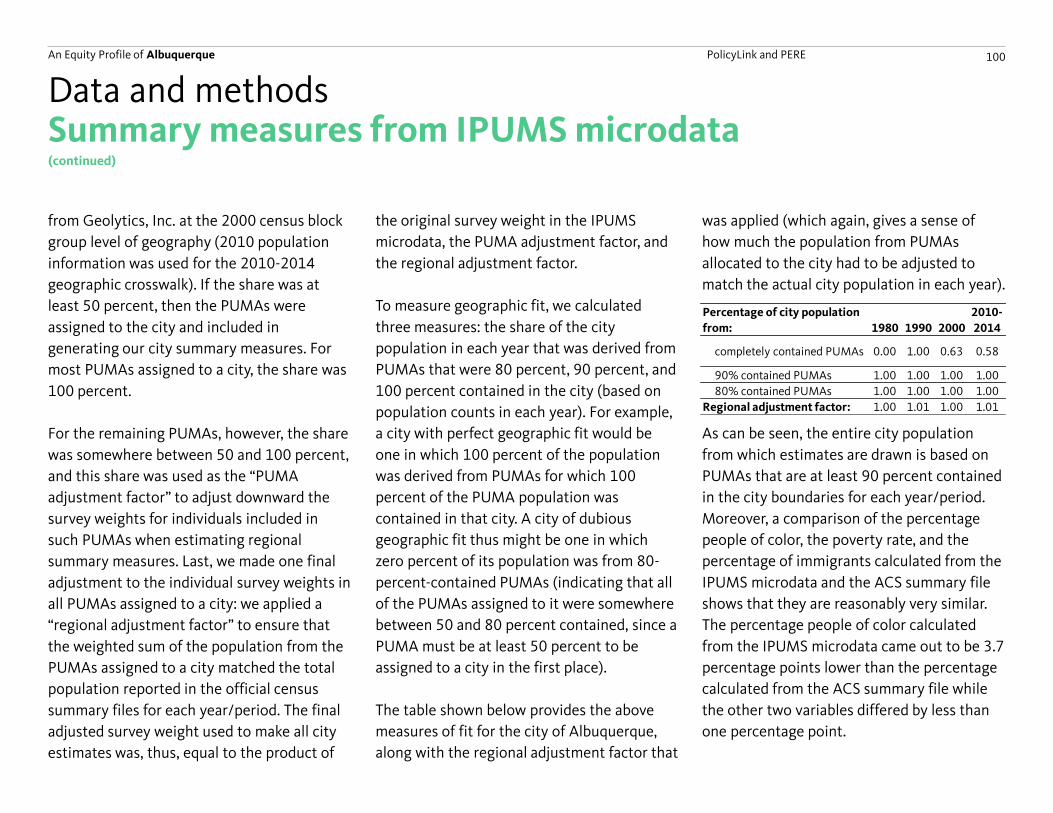
An Equity Profile of Albuquerque PolicyLink and PERE 100
was applied (which again, gives a sense of
how much the population from PUMAs
allocated to the city had to be adjusted to
match the actual city population in each year).
As can be seen, the entire city population
from which estimates are drawn is based on
PUMAs that are at least 90 percent contained
in the city boundaries for each year/period.
Moreover, a comparison of the percentage
people of color, the poverty rate, and the
percentage of immigrants calculated from the
IPUMS microdata and the ACS summary file
shows that they are reasonably very similar.
The percentage people of color calculated
from the IPUMS microdata came out to be 3.7
percentage points lower than the percentage
calculated from the ACS summary file while
the other two variables differed by less than
one percentage point.
Percentage of city population
from: 1980 1990 2000
2010-
2014
completely contained PUMAs 0.00 1.00 0.63 0.58
90% contained PUMAs 1.00 1.00 1.00 1.00
80% contained PUMAs 1.00 1.00 1.00 1.00
Regional adjustment factor: 1.00 1.01 1.00 1.01
Summary measures from IPUMS microdata
from Geolytics, Inc. at the 2000 census block
group level of geography (2010 population
information was used for the 2010-2014
geographic crosswalk). If the share was at
least 50 percent, then the PUMAs were
assigned to the city and included in
generating our city summary measures. For
most PUMAs assigned to a city, the share was
100 percent.
For the remaining PUMAs, however, the share
was somewhere between 50 and 100 percent,
and this share was used as the “PUMA
adjustment factor” to adjust downward the
survey weights for individuals included in
such PUMAs when estimating regional
summary measures. Last, we made one final
adjustment to the individual survey weights in
all PUMAs assigned to a city: we applied a
“regional adjustment factor” to ensure that
the weighted sum of the population from the
PUMAs assigned to a city matched the total
population reported in the official census
summary files for each year/period. The final
adjusted survey weight used to make all city
estimates was, thus, equal to the product of
Data and methods
the original survey weight in the IPUMS
microdata, the PUMA adjustment factor, and
the regional adjustment factor.
To measure geographic fit, we calculated
three measures: the share of the city
population in each year that was derived from
PUMAs that were 80 percent, 90 percent, and
100 percent contained in the city (based on
population counts in each year). For example,
a city with perfect geographic fit would be
one in which 100 percent of the population
was derived from PUMAs for which 100
percent of the PUMA population was
contained in that city. A city of dubious
geographic fit thus might be one in which
zero percent of its population was from 80-
percent-contained PUMAs (indicating that all
of the PUMAs assigned to it were somewhere
between 50 and 80 percent contained, since a
PUMA must be at least 50 percent to be
assigned to a city in the first place).
The table shown below provides the above
measures of fit for the city of Albuquerque,
along with the regional adjustment factor that
(continued)
An Equity Profile of Albuquerque PolicyLink and PERE 101
Adjustments made to census summary data on race/ethnicity by ageFor the racial generation gap indicator, we
generated consistent estimates of
populations by race/ethnicity and age group
(under 18, 18-64, and over 64 years of age)
for the years 1980, 1990, 2000, and 2014
(which reflects a 2010-2014 average), at the
city and county levels, which were then
aggregated to the regional level and higher.
The racial/ethnic groups include non-Hispanic
White, non-Hispanic Black, Hispanic/Latino,
non-Hispanic Asian and Pacific Islander, non-
Hispanic Native American/Alaska Native, and
non-Hispanic Other (including other single
race alone and those identifying as
multiracial, with the latter group only
appearing in 2000 and later due to a change
in the survey question). While for 2000 and
later years, this information is readily
available in SF1 and in the ACS, for 1980 and
1990, estimates had to be made to ensure
consistency over time, drawing on two
different summary files for each year.
For 1980, while information on total
population by race/ethnicity for all ages
combined was available at the city and county
Data and methods
levels for all the requisite groups in STF2, for
race/ethnicity by age group we had to look to
STF1, where it was only available for non-
Hispanic White, non-Hispanic Black, Hispanic,
and the remainder of the population. To
estimate the number of non-Hispanic Asian
or Pacific Islanders, non-Hispanic Native
Americans, and non-Hispanic Others among
the remainder for each age group, we applied
the distribution of these three groups from
the overall city and county populations
(across all ages) to that remainder.
For 1990, the level of detail available in the
underlying data differed at the city and
county levels, calling for different estimation
strategies. At the county level, data by
race/ethnicity was taken from STF2A, while
data by race/ethnicity and age was taken from
the 1990 MARS file—a special tabulation of
people by age, race, sex, and Hispanic origin.
However, to be consistent with the way race
is categorized by the OMB’s Directive 15, the
MARS file allocates all persons identifying as
“other race alone” or multiracial to a specific
race. After confirming that population totals
by county (across all ages) were consistent
between the MARS file and STF2A, we
calculated the number of “other race alone” or
multiracial people who had been added to
each racial/ethnic group in each county by
subtracting the number who were reported in
STF2A for the corresponding group. We then
derived the share of each racial/ethnic group
in the MARS file (across all ages) that was
made up of “other race alone” or multiracial
people and applied it to estimate the number
of people by race/ethnicity and age group
exclusive of “other race alone” or multiracial
people and the total number of “other race
alone” or multiracial people in each age
group.
For the 1990 city-level estimates, all data
were from STF1, which provided counts of the
total population for the six broad racial/ethnic
groups required but not counts by age. Rather,
age counts were only available for people by
single race alone (including those of Hispanic
origin) as well as for all people of Hispanic
origin combined. To estimate the number of
people by race/ethnicity and age for the six
An Equity Profile of Albuquerque PolicyLink and PERE 102
Adjustments made to census summary data on race/ethnicity by agebroad racial/ethnic groups that are detailed in
the profile, we first calculated the share of
each single-race alone group that was
Hispanic based on the overall population
(across all ages). We then applied it to the
population counts by age and race alone to
generate an initial estimate of the number of
Hispanic and non-Hispanic people in each
age/race alone category. This initial estimate
was multiplied by an adjustment factor
(specific to each age group) to ensure that the
sum of the estimated number of Hispanic
people across the race alone categories within
each age group equated to the “actual”
number of Hispanic origin by age as reported
in STF1. Finally, an Iterative Proportional
Fitting (IPF) procedure was applied to ensure
that our final estimate of the number of
people by race/ ethnicity and age was
consistent with the total population by
race/ethnicity (across all ages) and total
population by age group (across all
racial/ethnic categories) as reported in STF1.
Data and methods
(continued)
An Equity Profile of Albuquerque PolicyLink and PERE 103
Adjustments made to demographic projections
National projections
National projections of the non-Hispanic
White share of the population are based on
the U.S. Census Bureau’s 2014 National
Population Projections. However, because
these projections follow the OMB 1997
guidelines on racial classification and
essentially distribute the other single-race
alone group across the other defined
racial/ethnic categories, adjustments were
made to be consistent with the six
broad racial/ethnic groups used in our
analysis.
Specifically, we compared the percentage of
the total population composed of each
racial/ethnic group from the Census Bureau’s
Population Estimates program for 2015
(which follows the OMB 1997 guidelines) to
the percentage reported in the 2015 ACS 1-
year Summary File (which follows the 2000
Census classification). We subtracted the
percentage derived using the 2015
Population Estimates program from the
percentage derived using the 2015 ACS to
obtain an adjustment factor for each group
Data and methods
(all of which were negative, except for the
Mixed/other group) and carried this
adjustment factor forward by adding it to the
projected percentage for each group in each
projection year. Finally, we applied the
resulting adjusted projected population
distribution by race/ethnicity to the total
projected population from the 2014 National
Population Projections to get the projected
number of people by race/ethnicity in each
projection year.
County and regional projections
Similar adjustments were made in generating
county and regional projections of the
population by race/ethnicity. Initial county-
level projections were taken from Woods &
Poole Economics, Inc. Like the 1990 MARS
file described above, the Woods & Poole
projections follow the OMB Directive 15-race
categorization, assigning all persons
identifying as other or multiracial to one of
five mutually exclusive race categories: White,
Black, Latino, Asian or Pacific Islander, or
Native American. Thus, we first generated an
adjusted version of the county-level Woods &
Poole projections that removed the other or
multiracial group from each of these five
categories. This was done by comparing the
Woods & Poole projections for 2010 to the
actual results from SF1 of the 2010 Census,
figuring out the share of each racial/ethnic
group in the Woods & Poole data that was
composed of other or mixed-race persons in
2010, and applying it forward to later
projection years. From these projections, we
calculated the county-level distribution by
race/ethnicity in each projection year for five
groups (White, Black, Latino, Asian or Pacific
Islander, and Native American), exclusive of
other and mixed-race people.
To estimate the county-level share of
population for those classified as other or
mixed race in each projection year, we then
generated a simple straight-line projection of
this share using information from SF1 of the
2000 and 2010 Census. Keeping the
projected other or mixed race share fixed, we
allocated the remaining population share to
each of the other five racial/ethnic groups by
applying the racial/ethnic distribution implied
An Equity Profile of Albuquerque PolicyLink and PERE 104
Adjustments made to demographic projectionsData and methods
(continued)
by our adjusted Woods & Poole projections
for each county and projection year. The
result was a set of adjusted projections at the
county level for the six broad racial/ethnic
groups included in the profile, which were
then applied to projections of the total
population by county from the Woods & Poole
data to get projections of the number of
people for each of the six racial/ethnic
groups.
Finally, an Iterative Proportional Fitting (IPF)
procedure was applied to bring the county-
level results into alignment with our adjusted
national projections by race/ethnicity
described above. The final adjusted county
results were then aggregated to produce a
final set of projections at the regional, metro
area, and state levels.
An Equity Profile of Albuquerque PolicyLink and PERE 105
Estimates and adjustments made to BEA data on GDP
The data on national gross domestic product
(GDP) and its analogous regional measure,
gross regional product (GRP) – both referred
to as GDP in the text – are based on data from
the U.S. Bureau of Economic Analysis (BEA).
However, due to changes in the estimation
procedure used for the national (and state-
level) data in 1997, and a lack of metropolitan
area estimates prior to 2001, a variety of
adjustments and estimates were made to
produce a consistent series at the national,
state, metropolitan-area, and county levels
from 1969 to 2014.
Adjustments at the state and national levels
While data on gross state product (GSP) are
not reported directly in the profile, they were
used in making estimates of gross product at
the county level for all years and at the
regional level prior to 2001, so we applied the
same adjustments to the data that were
applied to the national GDP data. Given a
change in BEA’s estimation of gross product
at the state and national levels from a
standard industrial classification (SIC) basis to
a North American Industry Classification
Data and methods
System (NAICS) basis in 1997, data prior to
1997 were adjusted to prevent any erratic
shifts in gross product in that year. While the
change to a NAICS basis occurred in 1997,
BEA also provides estimates under an SIC
basis in that year. Our adjustment involved
figuring the 1997 ratio of NAICS-based gross
product to SIC-based gross product for each
state and the nation, and multiplying it by the
SIC-based gross product in all years prior to
1997 to get our final estimate of gross
product at the state and national levels.
County and metropolitan area estimates
To generate county-level estimates for all
years, and metropolitan-area estimates prior
to 2001, a more complicated estimation
procedure was followed. First, an initial set of
county estimates for each year was generated
by taking our final state-level estimates and
allocating gross product to the counties in
each state in proportion to total earnings of
employees working in each county – a BEA
variable that is available for all counties and
years. Next, the initial county estimates were
aggregated to metropolitan-area level, and
were compared with BEA’s official
metropolitan-area estimates for 2001 and
later. They were found to be very close, with a
correlation coefficient very close to one
(0.9997). Despite the near-perfect
correlation, we still used the official BEA
estimates in our final data series for 2001 and
later. However, to avoid any erratic shifts in
gross product during the years until 2001, we
made the same sort of adjustment to our
estimates of gross product at the
metropolitan-area level that was made to the
state and national data – we figured the 2001
ratio of the official BEA estimate to our initial
estimate, and multiplied it by our initial
estimates for 2000 and earlier to get our final
estimate of gross product at the
metropolitan-area level.
We then generated a second iteration of
county-level estimates – just for counties
included in metropolitan areas – by taking the
final metropolitan-area-level estimates and
allocating gross product to the counties in
each metropolitan area in proportion to total
earnings of employees working in each
An Equity Profile of Albuquerque PolicyLink and PERE 106
Estimates and adjustments made to BEA data on GDP
county. Next, we calculated the difference
between our final estimate of gross product
for each state and the sum of our second-
iteration county-level gross product estimates
for metropolitan counties contained in the
state (that is, counties contained in
metropolitan areas). This difference, total
nonmetropolitan gross product by state, was
then allocated to the nonmetropolitan
counties in each state, once again using total
earnings of employees working in each county
as the basis for allocation. Finally, one last set
of adjustments was made to the county-level
estimates to ensure that the sum of gross
product across the counties contained in each
metropolitan area agreed with our final
estimate of gross product by metropolitan
area, and that the sum of gross product across
the counties contained in state agreed with
our final estimate of gross product by state.
This was done using a simple IPF procedure.
The resulting county-level estimates were
then aggregated to the regional and metro
area levels.
We should note that BEA does not provide
Data and methods
data for all counties in the United States, but
rather groups some counties that have had
boundary changes since 1969 into county
groups to maintain consistency with historical
data. Any such county groups were treated
the same as other counties in the estimate
techniques described above.
(continued)
An Equity Profile of Albuquerque PolicyLink and PERE 107
Middle-class analysis
To analyze middle-class decline over the past
four decades, we began with the regional
household income distribution in 1979 – the
year for which income is reported in the 1980
Census (and the 1980 IPUMS microdata). The
middle 40 percent of households were
defined as “middle class,” and the upper and
lower bounds in terms of household income
(adjusted for inflation to be in 2010 dollars)
that contained the middle 40 percent of
households were identified. We then adjusted
these bounds over time to increase (or
decrease) at the same rate as real average
household income growth, identifying the
share of households falling above, below, and
within the adjusted bounds as the upper,
lower, and middle class, respectively, for each
year shown. Thus, the analysis of the size of
the middle class examined the share of
households enjoying the same relative
standard of living in each year as the middle
40 percent of households did in 1979.
Data and methods
An Equity Profile of Albuquerque PolicyLink and PERE 108
Assembling a complete dataset on employment and wages by industryAnalysis of jobs and wages by industry,
reported on pages 44-45, and 48-49, is based
on an industry-level dataset constructed
using two-digit NAICS industries from the
U.S. Bureau of Labor Statistics’ Quarterly
Census of Employment and Wages (QCEW).
Due to some missing (or nondisclosed) data
at the county and regional levels, we
supplemented our dataset using information
from Woods & Poole Economics, Inc., which
contains complete jobs and wages data for
broad, two-digit NAICS industries at multiple
geographic levels. (Proprietary issues barred
us from using Woods & Poole data directly, so
we instead used it to complete the QCEW
dataset.)
Given differences in the methodology
underlying the two data sources (in addition
to the proprietary issue), it would not be
appropriate to simply “plug in” corresponding
Woods & Poole data directly to fill in the
QCEW data for nondisclosed industries.
Therefore, our approach was to first calculate
the number of jobs and total wages from
nondisclosed industries in each county, and
Data and methods
then distribute those amounts across the
nondisclosed industries in proportion to their
reported numbers in the Woods & Poole data.
To make for a more accurate application of
the Woods & Poole data, we made some
adjustments to it to better align it with the
QCEW. One of the challenges of using Woods
& Poole data as a “filler dataset” is that it
includes all workers, while QCEW includes
only wage and salary workers. To normalize
the Woods & Poole data universe, we applied
both a national and regional wage and salary
adjustment factor; given the strong regional
variation in the share of workers who are
wage and salary, both adjustments were
necessary. Another adjustment made was to
aggregate data for some Woods & Poole
industry codes to match the NAICS codes
used in the QCEW.
It is important to note that not all counties
and regions were missing data at the two-
digit NAICS level in the QCEW, and the
majority of larger counties and regions with
missing data were only missing data for a
small number of industries and only in certain
years. Moreover, when data are missing it is
often for smaller industries. Thus, the
estimation procedure described is not likely
to greatly affect our analysis of industries,
particularly for larger counties and regions.
The same above procedure was applied at the
county and state levels. To assemble data at
for regions and metro areas, we aggregated
the county-level results.
An Equity Profile of Albuquerque PolicyLink and PERE 109
Growth in jobs and earnings by industry wage level, 1990 to 2015The analysis on pages 44-45 uses our filled-in
QCEW dataset (see the previous page) and
seeks to track shifts in regional job
composition and wage growth by industry
wage level.
Using 1990 as the base year, we classified all
broad private sector industries (at the two-
digit NAICS level) into three wage categories:
low-, middle-, and high-wage. An industry’s
wage category was based on its average
annual wage, and each of the three categories
contained approximately one-third of all
private industries in the region.
We applied the 1990 industry wage category
classification across all the years in the
dataset, so that the industries within each
category remained the same over time. This
way, we could track the broad trajectory of
jobs and wages in low-, middle-, and high-
wage industries.
Data and methods
This approach was adapted from a method
used in a Brookings Institution report by
Jennifer S. Vey, Building From Strength:
Creating Opportunity in Greater Baltimore's
Next Economy (Washington D.C.: Brookings
Institution, 2012).
While we initially sought to conduct the
analysis at a more detailed NAICS level, the
large amount of missing data at the three- to
six-digit NAICS levels (which could not be
resolved with the method that was applied to
generate our filled-in two-digit QCEW
dataset) prevented us from doing so.
An Equity Profile of Albuquerque PolicyLink and PERE 110
Analysis of occupations by opportunity levelData and methods
The analysis of occupations on pages 50-58
seeks to classify occupations in the region by
opportunity level. To identify “high-
opportunity” occupations, we developed an
“occupation opportunity index” based on
measures of job quality and growth, including
median annual wage, wage growth, job
growth (in number and share), and median
age of workers (which represents potential
job openings due to retirements). Once the
“occupation opportunity index” score was
calculated for each occupation, they were
sorted into three categories (high, middle, and
low opportunity). Occupations were evenly
distributed into the categories based on
employment.
There are some aspects of this analysis that
warrant further clarification. First, the
“occupation opportunity index” that is
constructed is based on a measure of job
quality and set of growth measures, with the
job-quality measure weighted twice as much
as all of the growth measures combined. This
weighting scheme was applied both because
we believe pay is a more direct measure of
“opportunity” than the other available
measures, and because it is more stable than
most of the other growth measures, which are
calculated over a relatively short period
(2005-2011). For example, an increase from
$6 per hour to $12 per hour is fantastic wage
growth (100 percent), but most would not
consider a $12-per-hour job as a “high-
opportunity” occupation.
Second, all measures used to calculate the
“occupation opportunity index” are based on
data for metropolitan statistical areas from
the Occupational Employment Statistics
(OES) program of the U.S. Bureau of Labor
Statistics (BLS), with one exception: median
age by occupation. This measure, included
among the growth metrics because it
indicates the potential for job openings due
to replacements as older workers retire, is
estimated for each occupation from the 2010
5-year IPUMS ACS microdata file (for the
employed civilian noninstitutional population
ages 16 and older). It is calculated at the
metropolitan statistical area level (to be
consistent with the geography of the OES
data), except in cases for which there were
fewer than 30 individual survey respondents
in an occupation; in these cases, the median
age estimate is based on national data.
Third, the level of occupational detail at which
the analysis was conducted, and at which the
lists of occupations are reported, is the three-
digit standard occupational classification
(SOC) level. While considerably more detailed
data is available in the OES, it was necessary
to aggregate to the three-digit SOC level in
order to align closely with the occupation
codes reported for workers in the ACS
microdata, making the analysis reported on
pages 55-58 possible.
Fourth, while most of the data used in the
analysis are regionally specific, information on
the education level of “typical workers” in
each occupation, which is used to divide
occupations in the region into the three
groups by education level (as presented on
pages 52-54), was estimated using national
2010 IPUMS ACS microdata (for the
employed civilian noninstitutional population
An Equity Profile of Albuquerque PolicyLink and PERE 111
Analysis of occupations by opportunity levelData and methods
ages 16 and older). Although regionally
specific data would seem to be the better
choice, given the level of occupational detail
at which the analysis is conducted, the sample
sizes for many occupations would be too
small for statistical reliability. And, while using
pooled 2006-2010 data would increase the
sample size, it would still not be sufficient for
many regions, so national 2010 data were
chosen given the balance of currency and
sample size for each occupation. The implicit
assumption in using national data is that the
occupations examined are of sufficient detail
that there is not great variation in the typical
educational level of workers in any given
occupation from region to region. While this
may not hold true in reality, it is not a terrible
assumption, and a similar approach was used
in a Brookings Institution report by Jonathan
Rothwell and Alan Berube, Education, Demand,
and Unemployment in Metropolitan America
(Washington D.C.: Brookings Institution,
September 2011).
We should also note that the BLS does publish
national information on typical education
needed for entry by occupation. However, in
comparing these data with the typical
education levels of actual workers by
occupation that were estimated using ACS
data, there were important differences, with
the BLS levels notably lower (as expected).
The levels estimated from the ACS were
determined to be the appropriate choice for
our analysis as they provide a more realistic
measure of the level of educational
attainment necessary to be a viable job
candidate – even if the typical requirement
for entry is lower.
Fifth, it is worthwhile to clarify an important
distinction between the lists of occupations
by typical education of workers and
opportunity level, presented on pages 52-54,
and the charts depicting the opportunity level
associated with jobs held by workers with
different education levels and backgrounds by
race/ethnicity, presented on pages 56-58.
While the former are based on the national
estimates of typical education levels
by occupation, with each occupation assigned
to one of the three broad education levels
described, the latter are based on actual
education levels of workers in the region (as
estimated using 2010 5-year IPUMS ACS
microdata), who may be employed in any
occupation, regardless of its associated
“typical” education level.
Lastly, it should be noted that for all of the
occupational analysis, it was an intentional
decision to keep the categorizations by
education and opportunity broad, with three
categories applied to each. For the
categorization of occupations, this was done
so that each occupation could be more
justifiably assigned to a single typical
education level; even with the three broad
categories some occupations had a fairly even
distribution of workers across them
nationally, but, for the most part, a large
majority fell in one of the three categories. In
regard to the three broad categories of
opportunity level and education levels of
workers, this was done to ensure reasonably
large sample sizes in the 2010 5-year IPUMS
ACS microdata that was used for the analysis.
(continued)
An Equity Profile of Albuquerque PolicyLink and PERE 112
Health data and analysisData and methods
While the data allow for the tabulation of
personal health characteristics, it is important
to keep in mind that because such tabulations
are based on samples, they are subject to a
margin of error and should be regarded as
estimates – particularly in smaller regions and
for smaller demographic subgroups.
To increase statistical reliability, we combined
five years of survey data, for 2008-2012. As
an additional effort to avoid reporting
potentially misleading estimates, we do not
report any estimates that are based on a
universe of fewer than 100 individual survey
respondents. This is similar to, but more
stringent than, a rule indicated in the
documentation for the 2012 BRFSS data of
not reporting (or interpreting) percentages
based on a denominator of fewer than 50
respondents (see:
https://www.cdc.gov/brfss/annual_data/2012
/pdf/Compare_2012.pdf). Even with this
sample size restriction, county and regional
estimates for smaller demographic subgroups
should be regarded with particular care.
Health data presented are from the
Behavioral Risk Factor Surveillance System
(BRFSS) database, housed in the Centers for
Disease Control and Prevention. The BRFSS
database is created from randomized
telephone surveys conducted by states, which
then incorporate their results into the
database on a monthly basis.
The results of this survey are self-reported
and the population includes all related adults,
unrelated adults, roomers, and domestic
workers who live at the residence. The survey
does not include adult family members who
are currently living elsewhere, such as at
college, a military base, a nursing home, or a
correctional facility.
The most detailed level of geography
associated with individuals in the BRFSS data
is the county. Using the county-level data as
building blocks, we created additional
estimates for the region, state, and country.
For more information and access to the BRFSS
database, see:
http://www.cdc.gov/brfss/index.html.
An Equity Profile of Albuquerque PolicyLink and PERE 113
Analysis of access to healthy food
Analysis of access to healthy food is based on
the 2014 Analysis of Limited Supermarket
Access (LSA) from the The Reinvestment Fund
(TRF). LSA areas are defined as one or more
contiguous census block groups (with a
collective population of at least 5,000) where
residents must travel significantly farther to
reach a supermarket than the “comparatively
acceptable” distance traveled by residents in
well-served areas with similar population
densities and car ownership rates.
The methodology’s key assumption is that
block groups with a median household
income greater than 120 percent of their
respective metropolitan area’s median (or
nonmetro state median for nonmetropolitan
areas) are adequately served by supermarkets
and thus travel an appropriate distance to
access food. Thus, higher-income block
groups establish the benchmark to which all
block groups are compared, controlling for
population density and car ownership rates.
Data and methods
An LSA score is calculated as the percentage
by which the distance to the nearest
supermarket would have to be reduced to
make a block group’s access equal to the
access observed for adequately served areas.
Block groups with an LSA score greater than
45 were subjected to a spatial connectivity
analysis, with 45 chosen as the minimum
threshold because it was roughly equal to the
average LSA score for all LSA block groups in
the 2011 TRF analysis.
Block groups with contiguous spatial
connectivity of high LSA scores are referred to
as LSA areas. They represent areas with the
strongest need for increased access to
supermarkets. Our analysis of the percent of
people living in LSA areas by race/ethnicity
and poverty level was done by merging data
from the 2014 5-year ACS summary file with
LSA areas at the block group level and
aggregating up to the city, county, and higher
levels of geography.
For more information on the 2014 LSA
analysis, see:
https://www.reinvestment.com/wp-
content/uploads/2015/12/2014_Limited_Sup
ermarket_Access_Analysis-Brief_2015.pdf.
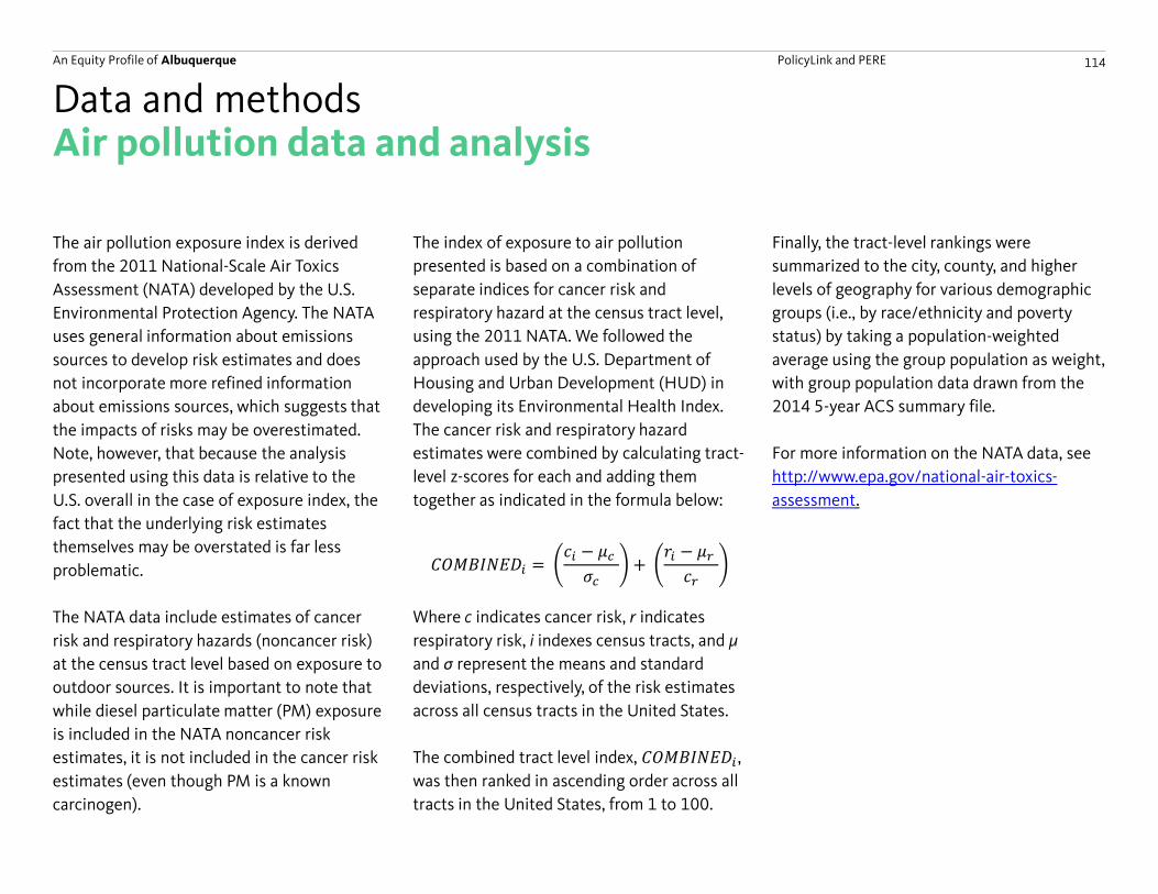
An Equity Profile of Albuquerque PolicyLink and PERE 114
Air pollution data and analysis
The air pollution exposure index is derived
from the 2011 National-Scale Air Toxics
Assessment (NATA) developed by the U.S.
Environmental Protection Agency. The NATA
uses general information about emissions
sources to develop risk estimates and does
not incorporate more refined information
about emissions sources, which suggests that
the impacts of risks may be overestimated.
Note, however, that because the analysis
presented using this data is relative to the
U.S. overall in the case of exposure index, the
fact that the underlying risk estimates
themselves may be overstated is far less
problematic.
The NATA data include estimates of cancer
risk and respiratory hazards (noncancer risk)
at the census tract level based on exposure to
outdoor sources. It is important to note that
while diesel particulate matter (PM) exposure
is included in the NATA noncancer risk
estimates, it is not included in the cancer risk
estimates (even though PM is a known
carcinogen).
Data and methods
The index of exposure to air pollution
presented is based on a combination of
separate indices for cancer risk and
respiratory hazard at the census tract level,
using the 2011 NATA. We followed the
approach used by the U.S. Department of
Housing and Urban Development (HUD) in
developing its Environmental Health Index.
The cancer risk and respiratory hazard
estimates were combined by calculating tract-
level z-scores for each and adding them
together as indicated in the formula below:
𝐶𝑂𝑀𝐵𝐼𝑁𝐸𝐷𝑖 =𝑐𝑖 − 𝜇𝑐𝜎𝑐
+𝑟𝑖 − 𝜇𝑟𝑐𝑟
Where c indicates cancer risk, r indicates
respiratory risk, i indexes census tracts, and µ
and σ represent the means and standard
deviations, respectively, of the risk estimates
across all census tracts in the United States.
The combined tract level index, 𝐶𝑂𝑀𝐵𝐼𝑁𝐸𝐷𝑖 ,
was then ranked in ascending order across all
tracts in the United States, from 1 to 100.
Finally, the tract-level rankings were
summarized to the city, county, and higher
levels of geography for various demographic
groups (i.e., by race/ethnicity and poverty
status) by taking a population-weighted
average using the group population as weight,
with group population data drawn from the
2014 5-year ACS summary file.
For more information on the NATA data, see
http://www.epa.gov/national-air-toxics-
assessment.
An Equity Profile of Albuquerque PolicyLink and PERE 115
Measures of diversity and segregation
In the profile, we refer to measures of
residential segregation by race/ethnicity (the
“multi-group entropy index” on page 77 and
the “dissimilarity index” on page 78). While
the common interpretation of these measures
is included in the text of the profile, the data
used to calculate them, and the sources of the
specific formulas that were applied, are
described below.
Both measures are based on census-tract-
level data for 1980, 1990, and 2000 from
Geolytics, and for 2014 (which reflects a
2010-2014 average) from the 2014 5-year
ACS. While the data for 1980, 1990, and 2000
originate from the decennial censuses of each
year, an advantage of the Geolytics data we
use is that it has been “re-shaped” to be
expressed in 2010 census tract boundaries,
and so the underlying geography for our
calculations is consistent over time; the
census tract boundaries of the original
decennial census data change with each
release, which could potentially cause a
change in the value of residential segregation
indices even if no actual change in residential
Data and methods
segregation occurred. In addition, while most
of the racial/ethnic categories for which
indices are calculated are consistent with all
other analyses presented in this profile, there
is one exception. Given limitations of the
tract-level data released in the 1980 Census,
Native Americans are combined with Asians
or Pacific Islanders in that year. For this
reason, we set 1990 as the base year (rather
than 1980) in the chart on page 78, but keep
the 1980 data in the chart on page 77 as this
minor inconsistency in the data is not likely to
affect the analysis.
The formula for the multi-group entropy index
was drawn from a 2004 report by John Iceland
of the University of Maryland, The Multigroup
Entropy Index (Also Known as Theil’s H or the
Information Theory Index) available at:
https://www.census.gov/topics/housing/hous
ing-patterns/about/multi-group-entropy-
index.html. In that report, the formula used to
calculate the multi-group entropy index
(referred to as the “entropy index” in the
report) appears on page 8.
The formula for the dissimilarity index is well
established, and is made available by the U.S.
Census Bureau at:
https://www.census.gov/library/publications/
2002/dec/censr-3.html.
An Equity Profile of Albuquerque PolicyLink and PERE 116
Estimates of GDP without racial gaps in income
Estimates of the gains in average annual
income and GDP under a hypothetical
scenario in which there is no income
inequality by race/ethnicity are based on the
2014 5-Year IPUMS ACS microdata. We
applied a methodology similar to that used by
Robert Lynch and Patrick Oakford in chapter
two of All-In Nation: An America that Works for
All, with some modification to include income
gains from increased employment (rather
than only those from increased wages). As in
the Lynch and Oakford analysis, once the
percentage increase in overall average annual
income was estimated, 2014 GDP was
assumed to rise by the same percentage.
We first organized individuals aged 16 or
older in the IPUMS ACS into six mutually
exclusive racial/ethnic groups: White, Black,
Latino, Asian or Pacific Islander, Native
American, and Mixed/other (with all defined
non-Hispanic except for Latinos, of course).
Following the approach of Lynch and Oakford
in All-In Nation, we excluded from the non-
Hispanic Asian/Pacific Islander category
subgroups whose average incomes were
Data and methods
higher than the average for non-Hispanic
Whites. Also, to avoid excluding subgroups
based on unreliable average income estimates
due to small sample sizes, we added the
restriction that a subgroup had to have at
least 100 individual survey respondents in
order to be included.
We then assumed that all racial/ethnic groups
had the same average annual income and
hours of work, by income percentile and age
group, as non-Hispanic Whites, and took
those values as the new “projected” income
and hours of work for each individual. For
example, a 54-year-old non-Hispanic Black
person falling between the 85th and 86th
percentiles of the non-Hispanic Black income
distribution was assigned the average annual
income and hours of work values found for
non-Hispanic White persons in the
corresponding age bracket (51 to 55 years
old) and “slice” of the non-Hispanic White
income distribution (between the 85th and
86th percentiles), regardless of whether that
individual was working or not. The projected
individual annual incomes and work hours
were then averaged for each racial/ethnic
group (other than non-Hispanic Whites) to
get projected average incomes and work
hours for each group as a whole, and for all
groups combined.
One difference between our approach and
that of Lynch and Oakford is that we include
all individuals ages 16 years and older, rather
than just those with positive income. Those
with income values of zero are largely non-
working, and were included so that income
gains attributable to increased hours of work
would reflect both more hours for the those
currently working and an increased share of
workers – an important factor to consider
given differences in employment rates by
race/ethnicity. One result of this choice is
that the average annual income values we
estimate are analogous to measures of per
capita income for the age 16- and-older
population and are thus notably lower than
those reported in Lynch and Oakford. Another
is that our estimated income gains are
relatively larger as they presume increased
employment rates.
An Equity Profile of Albuquerque PolicyLink and PERE 117
Estimates of GDP without racial gaps in income
Note that because no GDP data is available at
the city level (partly because economies tend
to operate at well beyond city boundaries),
our estimates of gains in GDP with racial
equity are only reported at the regional level.
Estimates of income gains and the source of
gains by race/ethnicity, however, are reported
for the profiled geography.
Data and methods
(continued)

Photo credits
Cover
Left photo: OpenThreads/ Flickr
Right photo: PolicyLink
Introduction
L: Robert Adams/Flickr
R: Robert Adams/Flickr
Demographics
L: National Nuclear Security
Administration/Flickr
R: Richie Diesterheft/Flickr
Economic vitality
L: Forever Southwest/Flickr
R: Jay Galvin/Flickr
Readiness
L: Carlos Villarreall/Flickr
R: Woody Hibbard/Flickr
Connectedness
L: Jacqueline Poggi/Flickr
R: Ron Cogswell/Flickr
Economic benefits
L: Archman8/Flickr
R: Richie Diesterheft/Flickr
Implications
L: Jay Rogers/Flickr
R: Siserrano/Flickr
This work is licensed under Creative Commons Attribution 4.0.
PolicyLink is a national research and action
institute advancing racial and economic
equity by Lifting Up What Works®.
Headquarters:
1438 Webster Street
Suite 303
Oakland, CA 94612
t 510 663-2333
f 510 663-9684
Communications:
75 Broad Street
Suite 701
New York, NY 10004
t 212 629-9570
f 212 730-2944
http://www.policylink.org
The USC Program for Environmental and
Regional Equity (PERE) conducts research and
facilitates discussions on issues of
environmental justice, regional inclusion, and
social movement building.
University of Southern California
950 W. Jefferson Boulevard
JEF 102
Los Angeles, CA 90089
t 213 821-1325
f 213 740-5680
http://dornsife.usc.edu/pere
©2018 by PolicyLink and PERE.
All rights reserved.