an equivalent isobaric geopotential height and its

VOLUME 127 FEBRUARY 1999M O N T H L Y W E A T H E R R E V I E W

q 1999 American Meteorological Society 145

An Equivalent Isobaric Geopotential Height and Its Application to Synoptic Analysisand a Generalized v Equation in s Coordinates

QIU-SHI CHEN AND DAVID H. BROMWICH

Polar Meteorology Group, Byrd Polar Research Center, The Ohio State University, Columbus, Ohio

(Manuscript received 30 April 1997, in final form 11 March 1998)

ABSTRACT

In s coordinates, a variable f e(x, y, s, t) whose horizontal gradient 2=f e is equal to the irrotational part ofthe horizontal pressure gradient force is referred to as an equivalent isobaric geopotential height. Its inner partcan be derived from the solution of a Poisson equation with zero Dirichlet boundary value. Because 2=f (x,y, p, t) is also the irrotational part of the horizontal pressure gradient force in p coordinates, the equivalentgeopotential f e in s coordinates can be used in the same way as the geopotential f (x, y, p, t) used in pcoordinates. In the sea level pressure (SLP) analysis over Greenland, small but strong high pressure systemsoften occur due to extrapolation. These artificial systems can be removed if the equivalent geopotential f e isused in synoptic analysis on a constant s surface, for example, at s 5 0.995 level. The geostrophic relationbetween the equivalent geopotential and streamfunction at s 5 0.995 is approximately satisfied.

Because weather systems over the Tibetan Plateau are very difficult to track using routine SLP, 850-hPa, and700-hPa analyses, equivalent isobaric geopotential analysis in s coordinates is especially useful over this area.An example of equivalent isobaric geopotential analysis at s 5 0.995 shows that a secondary high separatedfrom a major anticyclone over the Tibetan Plateau when cold air affected the northeastern part of the plateau,but this secondary high is hardly resolved by the SLP analysis. The early stage of a low (or vortex), called asouthwest vortex due to its origin in southwest China, over the eastern flank of the Tibetan Plateau is moreclearly identified by equivalent isobaric geopotential analysis at s 5 0.825 and 0.735 than by routine isobaricanalysis at the 850- and 700-hPa levels. Anomalous high and low systems in the SLP analysis over the TibetanPlateau due to extrapolation are all removed by equivalent isobaric geopotential analysis at s 5 0.995.

Use of equivalent geopotential f e in the vorticity and divergence equations is presented, and the equivalentgeopotential equation is derived. These equations can be used in numerical models, initializations, and otherdynamical studies. As an example, it is shown how these equations are used to derive a velocity potential formof the generalized v equation in s coordinates. As a check, retrieval of precipitation over Greenland using thisv equation shows that the computed precipitation distributions for 1987 and 1988 are in good agreement withthe observed annual accumulation.

1. Introduction

Synoptic and climatological analyses are very com-plicated in many high mountain regions, such as theTibetan Plateau, the Rocky Mountains, and westernUnited States (Sangster 1960, 1987; Harrison 1970; Hill1993). These analyses are also very difficult over Green-land and Antarctica due to the topography of the icesheets. The difficulty is caused by the fact that no singleelevation or pressure surface can be used to track sys-tems across the mountain region. Methods used to re-duce station pressure to sea level pressure (SLP) maynot be successful at capturing the isobaric pattern thatwould exist if the earth’s surface of the mountain region

Corresponding author address: Qiu-shi Chen, Byrd Polar ResearchCenter, The Ohio State University, 1090 Carmack Road, Columbus,OH 43210.E-mail: [email protected]

were at sea level. Thus, such an SLP pattern is oftennot representative of the true circulation that exists atground level across the elevated terrain.

The situation is perhaps worst over the Tibetan Pla-teau. The topography of east Asia is shown by Fig. 1aand it is derived from the U.S. Navy high-resolution109 3 109 dataset provided by the National Center forAtmospheric Research (NCAR). Figure 1a shows thatthe average elevation of the Tibetan Plateau is morethan 4000 m. Routine synoptic analyses at sea level andat the 850-and 700-hPa levels are all extrapolated fromthe upper troposphere and cannot track weather systemsover or moving across the Tibetan Plateau. However,such systems do exist and they often produce precipi-tation over Sichuan Basin and other downstream regionsafter they move away from the plateau.

The vertical coordinate s (Phillips 1957) defined bys 5 p/p*, where p*(x, y, t) is the pressure at the earth’ssurface, has been widely and successfully used to rep-resent orographic effects in numerical models, but it has

146 VOLUME 127M O N T H L Y W E A T H E R R E V I E W

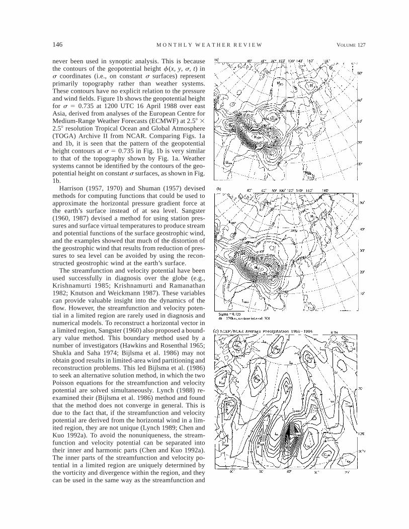
never been used in synoptic analysis. This is becausethe contours of the geopotential height f (x, y, s, t) ins coordinates (i.e., on constant s surfaces) representprimarily topography rather than weather systems.These contours have no explicit relation to the pressureand wind fields. Figure 1b shows the geopotential heightfor s 5 0.735 at 1200 UTC 16 April 1988 over eastAsia, derived from analyses of the European Centre forMedium-Range Weather Forecasts (ECMWF) at 2.58 32.58 resolution Tropical Ocean and Global Atmosphere(TOGA) Archive II from NCAR. Comparing Figs. 1aand 1b, it is seen that the pattern of the geopotentialheight contours at s 5 0.735 in Fig. 1b is very similarto that of the topography shown by Fig. 1a. Weathersystems cannot be identified by the contours of the geo-potential height on constant s surfaces, as shown in Fig.1b.

Harrison (1957, 1970) and Shuman (1957) devisedmethods for computing functions that could be used toapproximate the horizontal pressure gradient force atthe earth’s surface instead of at sea level. Sangster(1960, 1987) devised a method for using station pres-sures and surface virtual temperatures to produce streamand potential functions of the surface geostrophic wind,and the examples showed that much of the distortion ofthe geostrophic wind that results from reduction of pres-sures to sea level can be avoided by using the recon-structed geostrophic wind at the earth’s surface.

The streamfunction and velocity potential have beenused successfully in diagnosis over the globe (e.g.,Krishnamurti 1985; Krishnamurti and Ramanathan1982; Knutson and Weickmann 1987). These variablescan provide valuable insight into the dynamics of theflow. However, the streamfunction and velocity poten-tial in a limited region are rarely used in diagnosis andnumerical models. To reconstruct a horizontal vector ina limited region, Sangster (1960) also proposed a bound-ary value method. This boundary method used by anumber of investigators (Hawkins and Rosenthal 1965;Shukla and Saha 1974; Bijlsma et al. 1986) may notobtain good results in limited-area wind partitioning andreconstruction problems. This led Bijlsma et al. (1986)to seek an alternative solution method, in which the twoPoisson equations for the streamfunction and velocitypotential are solved simultaneously. Lynch (1988) re-examined their (Bijlsma et al. 1986) method and foundthat the method does not converge in general. This isdue to the fact that, if the streamfunction and velocitypotential are derived from the horizontal wind in a lim-ited region, they are not unique (Lynch 1989; Chen andKuo 1992a). To avoid the nonuniqueness, the stream-function and velocity potential can be separated intotheir inner and harmonic parts (Chen and Kuo 1992a).The inner parts of the streamfunction and velocity po-tential in a limited region are uniquely determined bythe vorticity and divergence within the region, and theycan be used in the same way as the streamfunction and

FEBRUARY 1999 147C H E N A N D B R O M W I C H

FIG. 1. (a) The topography of east Asia (in m with a contour intervalof 300 m). (b) The geopotential height, f(x, y, s, t), of the constant ssurface over east Asia at s 5 0.735 at 1200 UTC 16 April 1988 (in 10m2 s22 and contour interval: 300 3 10 m2 s22). (c) Mean annual pre-cipitation for 1982–94 computed by the NCEP–NCAR Reanalysis basedon a T62 model (in cm with a contour interval of 25 cm). (d) Observedannual mean precipitation distribution over Greenland from Ohmura andReeh (1991) in cm with a contour interval of 10 cm if smaller than 100cm, and 50 cm if larger than 100 cm. (e) The topography of Greenlandand adjacent areas (in m with a contour interval of 400 m).

velocity potential are used over the globe. This is dis-cussed in section 2.

In this paper, a new variable, f e, is proposed insteadof the geopotential height in s coordinates. The hori-zontal pressure gradient force in s coordinates can beseparated into its irrotational and rotational parts, wherethe irrotational part is denoted by 2=f e. If the vorticityand divergence equations are used, the irrotational androtational parts are always present independently inthese two equations. In p coordinates, 2=f (x, y, p, t)is also the irrotational part of the horizontal pressuregradient force; the irrotational part 2=f e in s coor-dinates can be used in the same manner as 2=f (x, y,p, t) is used in p coordinates. Thus, the variable f e isreferred to as an equivalent isobaric geopotential heightin s coordinates. Its analytic expression is given in sec-tion 3.

The geostrophic wind relation holds approximatelybetween the equivalent geopotential f e and the hori-zontal wind in s coordinates for synoptic-scale atmo-spheric motion in middle and high latitudes. The equiv-alent geopotential f e can be used to analyze weathersystems on constant s surfaces. This method is veryuseful near high mountains. Several synoptic examplesof this method over Greenland and the Tibetan Plateauare presented in section 4.

The equivalent geopotential f e in s coordinates canbe used not only in synoptic analysis but also in dynamicstudies. Use of the equivalent geopotential f e in thevorticity and divergence equations is discussed in sec-tion 5. In section 6, the equation for the equivalent geo-potential f e is developed. These equations can be usedin numerical models, initialization, and other dynamicalproblems. As a simple example, it is shown how theseequations are used in deriving a generalized v equationin s coordinates and how precipitation over Greenlandis retrieved using this derived equation.

Recently, climate change has been studied by ana-lyzing layers of ice from deep cores drilled from theGreenland Ice Sheet (e.g., Johnsen et al. 1992; Alley etal. 1993; Taylor et al. 1993). To help understand suchevents, it is necessary to investigate the present precip-itation characteristics over Greenland. The observationsof Greenland precipitation are limited and generally in-accurate (Bromwich and Robasky 1993). In particular,gauge measurements of the mostly solid precipitationare strongly contaminated by wind effects and are pri-marily confined to the complex coastal environment.Snow accumulation (the net result of precipitation, sub-limation/evaporation, and drifting) determinations fromthe ice sheet are limited in space and time. However,the analyzed wind, geopotential height, and moisturefields are available for recent years. The precipitationshould be retrievable from these fields by a dynamicapproach.

A natural method for retrieving precipitation overGreenland from the observed wind, geopotential height,and moisture fields is using a four-dimensional data as-


similation (FDDA) system. The National Centers forEnvironmental Prediction (NCEP) and NCAR (Kalnayet al. 1996) are cooperating in a project (denoted ‘‘re-analysis’’) to produce a 40-yr (1957–96) record of glob-al analyses of atmospheric fields, which includes theglobal recovery of precipitation. The model used fordata assimilation has a resolution of T62 (triangulartruncation at 62 waves), which is equivalent to about210 km, with 28 nonuniformly spaced vertical levels.

The mean annual precipitation over the Greenlandregion for 1982–94 from the reanalysis (Kalnay et al.1996) is shown in Fig. 1c. The observed mean annualprecipitation pattern over Greenland given by Ohmuraand Reeh (1991) is shown in Fig. 1d, which is basedon accumulation measurements of 251 pits and coreson the ice sheet and precipitation measurements at 35meteorological stations in the coastal region. From Fig.1c, it can be seen that a wave train pattern of the meanannual precipitation extends toward the southeast fromthe southeast coast. The topography over Greenland ispresented in Fig. 1e, and it shows that the slopes arevery steep near the southeast coast of Greenland. Thisquasi-stationary small-scale feature of the reanalysisprecipitation seems to be closely related to these steepslopes. Prevailing wisdom is that this precipitation pat-tern is the so-called spectral rain and it is a consequenceof the model’s inexact horizontal diffusion of humidityin the vicinity of steep mountain slopes (W. M. Ebi-suzaki 1996, personal communication).

It is seen that the highest amount of the mean annualprecipitation along the southeast coast in Fig. 1c is 388cm yr21, and the amounts are about twice those observedalong the southeast and southwest coasts (Fig. 1d).There is also a high precipitation area with a maximumof 110 cm yr21 in the central region of Greenland, wherethe observed accumulation is about 20 cm yr21 (Fig.1d). The NCEP–NCAR Reanalysis precipitation errorsover Greenland are much larger than those over thesoutheastern United States (Higgins et al. 1996). Exceptfor some effects of inaccurate observation over Green-land, these larger errors are probably caused, as men-tioned before, by the numerical model’s inability to dealproperly with the steep slopes near the coast of Green-land.

It is interesting to know whether the capability of anumerical model in dealing with complicated mountainsis improved if the equivalent isobaric geopotential isused. However, FDDA systems for limited regions arestill under development, and they are computationallyvery demanding. Because we only want to determinesome basic features of precipitation over Greenland, therelatively simple approach used by Bromwich et al.(1993) is adopted. Bromwich et al. (1993) applied asimplified quasigeostrophic v equation in p coordinateswith a statistical method to calculate the annual precip-itation over the Greenland Ice Sheet. The major short-coming of their simulated precipitation over Greenlandis caused by orographic effects.

Because the quasigeostrophic approximation is notaccurate enough, a number of generalized v equationswith fewer assumptions have been developed (e.g.,Krishnamurti 1968a,b; Tarbell et al. 1981; DiMego andBosart 1982; Iversen and Nordeng 1984; Hirschberg andFritsch 1991; Pauley and Nieman 1992; Raisanen 1995).However, the quasigeostrophic v equation and its gen-eralizations always use p coordinates, and its boundarycondition at the earth’s surface is usually given by thatat p 5 1000 hPa, w 5 V · =H*, where w is the verticalvelocity and H* is the elevation of the earth’s surface.Under this boundary condition, it is necessary to cal-culate the vorticity and temperature advections at the850 hPa and other lower levels in deriving the solutionof the v equation. These advections cannot be computedcorrectly over Greenland because the 850 hPa and otherlower levels are actually below the earth’s surface. Thus,the solution of the quasigeostrophic v equation in pcoordinates cannot be derived accurately over Green-land. In this case, the equivalent geopotential f e is usedto develop a generalized v equation without the qua-sigeostrophic approximation in s coordinates to im-prove the retrieval of precipitation over Greenland.

By means of the equivalent geopotential f e, a velocitypotential form of the generalized v equation without thequasigeostrophic approximation in s coordinates and itssolution are shown in section 7. Some test results forprecipitation over Greenland are presented in section 8.

2. Inner part analysis

a. Use of the inner parts of the streamfunction andvelocity potential in a limited region

In coordinates of a conformal map projection, let U,V, V, D be

u y z dU 5 , V 5 , V 5 , D 5 , (2.1)

2 2m m m m

where u and y are the horizontal components of thewind field, z the vertical component of the vorticity, dthe horizontal divergence, and m the map scale factor.The horizontal wind components are expressed by:

]c ]x ]c ]xU 5 2 1 , V 5 1 , (2.2)

]y ]x ]x ]y

where the streamfunction c and velocity potential xsatisfy the following Poisson equations,

¹2c 5 V, ¹2x 5 D, (2.3)

within the limited region, and at the boundary they sat-isfy the conditions

]c ]xs · V 5 1 5 V ,t]n ]s

]c ]xn · V 5 2 1 5 V . (2.4)n]s ]n


Here s and n are tangential and normal unit vectors,respectively, and s and n are distances along and normalto the boundary.

The partitioning problem in a limited region is tosolve the streamfunction and velocity potential from thetwo Poisson equations (2.3) with boundary conditions(2.4). The conditions (2.4) are referred to as coupledboundary conditions because the normal and tangentialderivatives are coupled together (Chen and Kuo 1992b).They are neither Dirichlet nor Neumann boundary con-ditions. This partitioning problem is a special problemof mathematical physics.

Lynch (1989) and Chen and Kuo (1992a) found thatpartitioning the wind in a limited region into nondiv-ergent and irrotational components is not unique. Thenonuniqueness is closely related to a portion of the windbeing both nondivergent and irrotational in a limitedregion. A limited region, R, is only a portion of theglobal area. The region over the globe outside regionR is referred to as an external region. From a globalperspective, the streamfunction and velocity potential,as well as the horizontal wind, in region R depend uponthe vorticity and divergence not only within region Rbut also in the external region. The portion of the windfield that is both nondivergent and irrotational withinregion R is referred to as an external wind. Due to theproperties of nondivergence and irrotation, no matterhow the vorticity and divergence vary within the regionR, the external wind does not change. Thus, the externalwind has no relation to the vorticity and divergencewithin the region R. However, from a global view, theexternal wind must depend only on the vorticity anddivergence in the external region, which is why it iscalled the ‘‘external’’ wind. For the global area, a bothnondivergent and irrotational wind is always zero, thusthe external wind must vanish, and also there is noexternal region.

To enable the streamfunction and velocity potentialin a limited region to be used as conveniently as thoseused on the globe and to avoid the nonuniqueness, Chenand Kuo (1992a) separated the streamfunction and ve-locity potential in a limited region into the inner andharmonic parts as

c 5 c i 1 ch, x 5 x i 1 xh, (2.5)

where the inner parts, c i and xi, satisfy the Poissonequations

¹2ci 5 V, ¹2xi 5 D (2.6)

with zero Dirichlet boundary value. The wind computedfrom the inner part as

]c ]x ]c ]xi i i iU 5 2 1 , V 5 1 . (2.7)I I]y ]x ]x ]y

is called an internal wind. Because the solution of aPoisson equation with a Dirichlet boundary value isunique, these inner parts and the internal wind areuniquely determined by the vorticity and divergence

within the limited region R. No matter how the vorticityand divergence vary in the external region (outside theregion R), the inner parts of the streamfunction andvelocity potential, as well as the internal wind, do notvary.

The difference between the wind and internal windcan be expressed by

UE 5 U 2 UI, VE 5 V 2 VI. (2.8)

According to (2.2) and (2.7), the relationship betweenVE and the harmonic parts of the streamfunction andvelocity potential is expressed by

]c ]x ]c ]xh h h hU 5 2 1 , V 5 1 . (2.9)E E]y ]x ]x ]y

From (2.3) and (2.6), the harmonic parts satisfy Laplaceequations

¹2ch 5 0, ¹2xh 5 0 (2.10)

with the coupled boundary conditions

]c ]xh hU | 5 2 1 ,E S 1 2)]y ]xS

]c ]xh hV | 5 1 . (2.11)E S 1 2)]x ]yS

The wind VE that satisfies (2.9), (2.10), and (2.11)must be both nondivergent and irrotational within thelimited region R, thus it must be the external wind. Byusing the above method, the external wind can be sep-arated from the wind field in a limited region.

The above method is used to separate the horizontalwind into the internal and external wind. The internalwind can be further separated into its internal nondiv-ergent and irrotational components based on (2.7). Thus,the horizontal wind in a limited area is expressed by asum of three parts as

V 5 k 3 =ci 1 =xi 1 VE, (2.12)

where k 3 =c i is the internal nondivergent componentand =xi is the internal irrotational component. Becausethe inner parts of the streamfunction and velocity po-tential are uniquely determined in a limited region, theycan be used in the same way as the streamfunction andvelocity potential are used on the globe. The internalwind in a limited region is dealt with the same as thehorizontal wind on the globe. Using the above methodin (2.12), any horizontal vector in a limited region canbe separated into its internal nondivergent, internal ir-rotational, and external components.

b. The inner part of the geopotential height

The geopotential height on the constant s surface ina limited region can also be separated into the harmonicand inner parts,


f 5 f h(x, y, s, t) 1 f i(x, y, s, t), (2.13)

where its harmonic part satisfies the Laplace equation

¹2f h(x, y, s, t) 5 0 (2.14)

with the Dirichlet boundary value of the geopotentialheight itself as

f h|S 5 f |S, (2.15)

and its inner part is derived from the difference betweenf and its harmonic part,

f i 5 f 2 f h. (2.16)

If the Laplacian of geopotential heght, ¹2f, is knownin a limited region, the inner part can also be derivedfrom the Poisson equation

¹2f i 5 (¹2f )(x, y) (2.17)

with zero Dirichlet boundary value. Here the right-handside of (2.17) is a known function in the region.

If an equation A 5 B is satisfied in a limited regionand both sides of the equation are separated into theirinner and harmonic parts, the following equations

Ah 5 Bh and Ai 5 Bi, (2.18)

are satisfied in the limited region based on the unique-ness of a harmonic function with a Dirichlet boundaryvalue.

c. Inner part analysis

If a limited-area model is formulated in terms of thevorticity and divergence equations and is nested in aglobal model by the one-way method, at each time steponly the vorticity and divergence within the region canbe predicted by the limited-area model. This means thatonly the internal wind and inner parts can be predictedfrom the limited-area model, whereas the external windand harmonic parts must be derived from the predictionof the global model. In this case, the external wind andharmonic parts can be used as the lateral boundary con-dition for the limited-area model. This method has beensuccessfully used in the harmonic-Fourier spectral lim-ited-area model studied by Chen et al. (1997a) (hereafterreferred to as CBB), and very good predicted resultshave been obtained.

The predicted variables of this limited-area model arethe inner parts of the streamfunction, velocity potential,and geopotential height, and they describe the devel-opment of motion systems very well in the model. Thus,these inner parts must be able to be used in synopticanalysis of a limited region. A method of using the innerparts of the streamfunction, velocity potential, and othervariables to describe motion systems in a limited regionis referred to as inner part analysis.

The inner part variables are dependent on the hori-zontal scale of the limited region chosen for study, thus,the horizontal scale of the studied region must be chosen

to be large enough so that the studied motion systemsare completely described by the vorticity and divergencewithin the region. The harmonic parts and the compo-nents of the external wind are all harmonic functions inthe limited domain. These harmonic functions attaintheir largest and smallest values at the boundary, andtheir horizontal scale must be larger than that of thelimited region. Thus, the horizontal scale of the har-monic parts and external wind are much larger thanthose of the motion systems studied in the limited re-gion.

3. An equivalent isobaric geopotential height ins coordinates

a. Definition of equivalent isobaric geopotentialheight

The horizontal pressure gradient force in p coordi-nates is expressed by 2=f (x, y, p, t), where f (x, y, p,t) is the geopotential height in p coordinates. When itis transformed into s coordinates, it is expressed by

G 5 2=f(x, y, s, t)

2 RT(x, y, s, t)= lnp (x, y, t), (3.1)*

where G denotes the horizontal pressure gradient force,and f (x, y, s, t) is the geopotential height in s coor-dinates. It is seen that the vector 2=f (x, y, p, t) isirrotational, but the total vector on the right-hand sideof (3.1) is not irrotational because T is a function of xand y.

Similar to the pressure gradient force in p coordinates,we can look for a vector expressed by 2=f e(x, y, s,t) that represents the irrotational part of the horizontalpressure gradient force in s coordinates. In this case,the irrotational part of 2=f e(x, y, s, t) must be equalto the irrotational part of the total vector on the right-hand side of (3.1), thus we have

] ] lnp ] ] lnp2 2 * *¹ f 5 ¹ f 1 RT 1 RT .e 1 2 1 2]x ]x ]y ]y

(3.2)

The total vector on the right-hand side of (3.1) has arotational part. The irrotational and rotational parts ofthe horizontal pressure gradient force are independentof each other in the divergence and vorticity equations.The rotational part is very small, and it is proved in thenext section that the magnitude of the rotational part isone order smaller than the irrotational part even overhigh mountain regions. The irrotational part 2=f e canbe used in s coordinates in the same way as 2=f (x,y, p, t) is used in p coordinates. Thus, the variable f e

is referred to as an equivalent isobaric geopotentialheight, or briefly, an equivalent geopotential in s co-ordinates.

Over the globe, the Poisson equation (3.2) is easily


solved without lateral boundary conditions. If equation(3.2) needs to be solved in a limited region, similar to(2.13), the equivalent geopotential in s coordinates canbe separated into its inner and harmonic parts as

f e 5 f ei(x, y, s, t) 1 f eh(x, y, s, t). (3.3)

Based on (3.2), the inner part of the equivalent geo-potential, f ei , in s coordinates can be derived from thesolution of the following Poisson equation

] ] lnp ] ] lnp2 2 * *¹ f 5 ¹ f 1 RT 1 RTei i 1 2 1 2]x ]x ]y ]y

(3.4)

with zero Dirichlet boundary value. The solution of(3.4) can be expressed by

] ] lnp ] ] lnp22 * *f 5 f 1 = RT 1 RT , (3.5)ei i 1 2]x ]x ]y ]y

where ¹22 is an integral operator shown in the appendixto denote the solution of the Poisson equation with zeroDirichlet boundary value. From (3.5), the inner part ofthe equivalent geopotential f ei can be derived.

b. Physical interpretation of the equivalentgeopotential height

To show the physical basis for f e, (3.4) can be re-written as

2 2¹ (f 2 f ) 5 ¹ fi ei ci

] ] lnp ] ] lnp* *5 2 RT 2 RT1 2 1 2]x ]x ]y ]y

5 = · (2RT= lnp ), (3.6)*

where f ci 5 f i 2 f ei is a potential function of thevector 2RT= lnp*.

The horizontal gradient of the surface pressure p*(x,y, t) caused by topography is much larger than by thatcaused by synoptic disturbances, especially near highmountain regions. Thus, the contours of the height ofthe earth’s surface, H*(x, y), are roughly parallel to thecontours of p* or lnp*. A low value center of p* or lnp*is located in the region where H*(x, y) is high. Thevector 2RT= lnp* has the direction from high valuesof lnp* to low values. Thus, over a high mountain re-gion, the vector 2RT= lnp* must converge, that is,= · (2RT = lnp*) , 0. If this distribution of= · (2RT= lnp*) is solved from the Poisson equation(3.6), f ci must have a positive center over the highmountain region. (It is easy to estimate the solution ofthe Poisson equation because the solution is an inverseoperator of the Lapalacian operator ¹2.) The potentialfunction f ci has the property that =f ci 5 2RT= lnp*.Thus, =f ei 5 =f i 2 =f ci . The potential function f ci

acts to reduce the value of f (x, y, s, t) to f e(x, y, s,

x), and to make =f e(x, y, s, t) equal to the irrotationalpart of the horizontal pressure gradient force.

The physical implication of f e can also be understoodfrom a comparison between f (x, y, s, t) and f (x, y, p,t). In s coordinates, the earth’s surface is a coordinatesurface. The major difference between f (x, y, s, t) andf (x, y, p, t) is that =f (x, y, s, t) is not equal to thehorizontal pressure gradient force because f (x, y, s, t)has been altered by orography. The value of f (x, y, s,t) is computed from the hydrostatic equation in s co-ordinates. The topography has two ways to affect thecomputation of f (x, y, s, t). One is through the initialvalue f*, where f* 5 gH* is used in the integrationof the hydrostatic equation. This is the direct effect fromthe topography itself. The second effect is indirectlythrough the temperature T(x, y, s, t), where the tem-perature used in the integration in s coordinates hasbeen altered by orography.

Equation (3.6) can be rewritten as

¹2f ci 5 2RT¹2 lnp* 2 R=T · = lnp*. (3.7)

As mentioned above, a low value center of p* or lnp*is located over a mountain region where the elevationis high. Over the high mountain region, ¹2 lnp* . 0and 2RT¹2 lnp* , 0 due to the low value center oflnp*.

The temperature T(x, y, s, t) in s coordinates can beseparated into two parts as

T(x, y, s, t) 5 Tor 1 TSL, (3.8)

where TSL(x, y, s, t) is the temperature that is not af-fected by orography. It is the temperature in s coor-dinates if p* 5 p0(x, y, t), where p0(x, y, t) is the SLPat H* 5 0, and it is equivalent to the temperature in pcoordinates. From (3.8), we have Tor 5 T(x, y, s, t) 2TSL, where Tor is the temperature caused by orography.If p* 5 p0(x, y, t) at H* 5 0, then T(x, y, s, t) 5 TSL,and Tor 5 0. The temperature Tor is the major differencebetween T(x, y, s, t) and T(x, y, p, t). The temperatureTSL can further be divided into three parts as

T (x, y, s, t) 5 T (s) 1 T (x, y, s)SL 0 cl

1 T (x, y, s, t), (3.9)sy

where T0(s) is the mean value of TSL averaged over theconstant s surface, Tcl is temperature deviation causedby climate without the effect of orography (equivalentto the climate state in p coordinates), and Tsy is causedby the transient synoptic disturbances.

The temperature caused by orography, Tor, is pro-duced through temperature decrease with height. Thehorizontal temperature gradient caused by orography,=Tor, is the major part of the temperature gradient nearhigh mountain regions. The isotherms for Tor are almostparallel to the contours of lnp* over high mountain re-gions. The cold center of Tor is located in the regionwhere lnp* is low (or the elevation is high). Over a highmountain region, the vectors =Tor and = lnp* have the


same direction, thus 2R=Tor · = lnp* , 0, and its larg-est negative value is over steep slopes, where the ab-solute values of both =Tor and = lnp* are very large.

If the sum of the two terms on the right-hand side of(3.7) is solved from this Poisson equation, f ci has apositive center over the high mountain region. In theregion where the effect of topography is small, =p*(x,y, t) and =Tor are both very small, the value of f ci isalso very small, and vice versa. Thus, the distributionof f ci produced by the two terms on the right-hand sideof (3.7) mainly represents the part of f (x, y, s, t) thatis produced by the effects of topography. These effectsinclude those directly from terrain itself, =p*, and in-directly from the temperature field, =Tor.

The equation f ei 5 f i 2 f ci means that the part ofgeopotential produced by the effect of topography, f ci ,is removed from f (x, y, s, t), and the remainder is f e.Thus, the equivalent geopotential f e is similar to f (x,y, p, t), which is not affected by topography. The equiv-alent geopotential f e is a variable in s coordinates, butit plays the same role as the geopotential height f (x, y,p, t) does in p coordinates.

c. The geostrophic approximation for the rotationalwind in s coordinates

In s coordinates, where s 5 p/p*, the momentumequation is expressed by

]V ]V1 V · =V 1 s 1 f k 3 V

]t ]s

5 =f 2 RT= lnp 1 P, (3.10)*

where P is the friction caused by the vertical fluxes ofmomentum due to convection and boundary layer tur-bulence. The geostrophic wind approximation in s co-ordinates can be denoted by

f k 3 V ù 2=f 2 RT = lnp*. (3.11)

The horizontal pressure gradient force in the right-hand side of (3.11) can be partitioned into the irrota-tional and rotational parts, and (3.11) can be written as

f k 3 V ù 2=f e 2 k 3 =h, (3.12)

where 2k 3 =h is the rotational part of the horizontalpressure gradient force, and h is referred to as a geo-streamfunction. Equation (3.12) is similar to that usedby Sangster (1960) to compute the surface geostrophicwind over mountain regions. The geo-streamfunctionsatisfies

]T ] lnp ]T ] lnp2 * *¹ h 5 R 2 (3.13)1 2]x ]y ]y ]x

without the boundary condition over the globe. If equa-tion (3.13) is solved in a limited region, the geo-stream-function can also be separated into its inner and har-monic parts, then the inner part of the geo-streamfunc-

tion, hi, can be derived from the following Poissonequation

]T ] lnp ]T ] lnp2 * *¹ h 5 R 2 (3.14)i 1 2]x ]y ]y ]x

with zero Dirichlet boundary value. Equation (3.12) canbe rewritten as

u 1 ]f 1 ]heU 5 ù 2 1 ,m f ]y f ]x0 0

y 1 ]f 1 ]heV 5 ù 1 . (3.15)m f ]x f ]y0 0

From (3.15), the vorticity is approximately expressedby

12 2V 5 ¹ c ù ¹ f . (3.16)ef0

In (3.16), only the irrotational part of the horizontalpressure gradient force is considered, and the rotationalpart is eliminated automatically. Equation (3.16) can besolved with zero Dirichlet boundary value in a limitedregion, and its solution is

f 0ci ù f ei. (3.17)

Equation (3.17) is the geostrophic approximation for therotational wind in s coordinates.

4. Some examples of synoptic analysis using theequivalent isobaric geopotential in scoordinates

a. A synoptic example over Greenland analyzed bythe inner part of the equivalent isobaricgeopotential at s 5 0.995

The equivalent isobaric geopotential height can beused in synoptic analysis over orographically compli-cated regions, such as Greenland and the Tibetan Pla-teau. The topography of the studied region near Green-land is presented in Fig. 1e. Data from ECMWF at 2.583 2.58 resolution (TOGA Archive II from NCAR) areinterpolated to 16 s levels in the vertical, at s 5 0.015,0.045, 0.075, 0.105, 0.140, 0.200, 0.285, 0.390, 0.510,0.630, 0.735, 0.825, 0.900, 0.950, 0.980, and 0.995. Themesh size of the limited region used in analysis is 1113 81 and the grid spacing is 50 km.

In Greenland, snow and ice surfaces typically havean albedo larger than 0.80, implying that more thanthree-quarters of the incident shortwave radiation fromthe sun are reflected. Little of this reflected solar radi-ation is absorbed by the overlying atmosphere. In ad-dition, the ice surface acts nearly like a blackbody forlongwave radiation. Thus, the ice surface efficiently ra-diates thermal energy to outer space. The cold sourceat the ice and snow surface will reduce the air temper-ature in the boundary layer by downward sensible heat


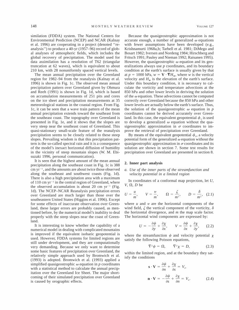
FIG. 2. (a) The inner part of the equivalent isobaric geopotentialheight at 0000 UTC 8 January 1992 at s 5 0.995 (in 10 m2 s22 andcontour interval: 40 3 10 m2 s22). (b) Same as (a) except for 1200UTC 8 January 1992. (c) Same as (a) except for 0000 UTC 9 January1992. (d) Same as (a) except for 1200 UTC 9 January 1992. (e) SLPat 0000 UTC 8 January 1992 (5-hPa isobar spacing). (f ) Same as (e)except for 1200 UTC 8 January 1992. (g) Same as (e) except for0000 UTC 9 January 1992. (h) Same as (e) except for 1200 UTC 9January 1992. (i) The inner part of the geo-streamfunction at 1200UTC 8 January 1992 at s 5 0.995 (in 10 m2 s22 and contour interval:20 3 10 m2 s22). (j) Same as (i) except for 1200 UTC 9 January1992. (k) Schematic diagram of a mountain with an idealized ellipticalshape and a temperature field that decreases with latitude.


FIG. 2 (Continued) (l) The inner part of the streamfunction at 1200 UTC 8 January 1992 at s 5 0.995 (in 106 m2 s21 and contour interval:2 3 106 m2 s21). (m) Same as (i) except for 1200 UTC 9 January 1992. (n) The inner part of the velocity potential at 1200 UTC 8 January1992 at s 5 0.995 (in 106 m2 s21 and contour interval: 2 3 106 m2 s21). (o) Same as (n) except for 1200 UTC 9 January 1992.

transfer. Thus, a cold high pressure system is often lo-cated over Greenland if the circulation is not disturbedby synoptic systems.

The inner part of the equivalent isobaric geopotentialheight computed from (3.5) at s 5 0.995 for 0000 UTC8 January 1992 is shown in Fig. 2a. In Fig. 2a, there isan anticyclone over most of Greenland. A cyclone lo-cated in the Labrador Sea is moving eastward towardthe southwest coast of Greenland, and another cycloniccenter is over Baffin Bay.

The inner part of the equivalent isobaric geopotentialheight at s 5 0.995 for 1200 UTC 8 and 0000 and 1200UTC 9 January 1992 are presented in Figs. 2b–d, re-spectively. The Labrador Sea cyclone reaches the south-west coast of Greenland in the next 12 h as shown inFig. 2b, and the anticyclone weakens to a high pressure

ridge over the east coast. In Figs. 2c and 2d, the centerof the equivalent geopotential low has moved to thesoutheast coast and develops on the lee side of the south-ern part of Greenland, respectively. At the same time,the cyclone in Baffin Bay moves northward, weakens,and dissipates.

The SLP analyses at 0000 UTC and 1200 UTC 8January and 0000 and 1200 UTC 9 January 1992 arepresented in Figs. 2e–h, respectively. These analyses aredirectly based on ECMWF analysis and we do not sep-arate the inner and harmonic parts of the SLP. Becausethe harmonic parts are the harmonic functions and attaintheir largest and smallest values at the boundary, theirabsolute values in the inner region are relatively small.Thus, only the inner region of Figs. 2e–h can be usedfor comparison with Figs. 2a–d, which represent only


the inner parts of the equivalent geopotential solvedfrom (3.4) with zero Dirichlet boundary value. The innerregion of Figs. 2e–h over the oceanic region outsideGreenland are very similar to Figs. 2a–d, respectively.The development and displacement of the cyclone ini-tially located over the Labrador Sea are the same asthose shown in Figs. 2a–d. However, there are manysmall but strong high centers (as well as low centers)in these SLP maps over Greenland shown in Figs. 2e–h. These are major differences between the analyses ofthe equivalent isobaric geopotential and of the SLP overGreenland. These small but strong high pressure systemsare caused by reduction of pressure to sea level usingcold temperatures at the top of the ice sheet. Thesesystems do not exist in the real atmosphere. If the equiv-alent isobaric geopotential at s 5 0.995 is used as shownin Figs. 2a–d, these small but strong high pressure sys-tems over Greenland are all removed. The circulationat s 5 0.995 becomes very smooth and it representsthe true circulation that exists near the ground of theGreenland Ice Sheet.

Details about how to separate a variable into its innerand harmonic parts and how to derive the solution ofthe Poisson equation to perform synoptic analyses arethe same as those discussed by Chen and Kuo (1992a)and Chen et al. (1997a). The harmonic-sine spectralmethod is used in all of these computations. These com-putations can also be implemented by a finite-differencemethod.

b. Some characteristics of the geo-streamfunction andthe geostrophic approximation in s coordinates

Figures 2i and 2j are the inner part of the geo-stream-function at s 5 0.995 level for 1200 UTC 8 and 9January 1992, respectively. They are derived from(3.14) with zero Dirichlet boundary value. The times ofFigs. 2i and 2j are the same as those of Figs. 2b and2d. From Figs. 2b and 2d, it can be seen that a cyclonedevelops in Fig. 2d on the east coast of Greenland inplace of the high pressure ridge shown in Fig. 2b, where-as Figs. 2i and 2j do not show important changes inthese two features. The fields shown in Figs. 2i and 2jlook the same; there is a low of the geo-streamfunctionon the east coast of Greenland and a high in the west.We cannot find clear relationship between the geo-streamfunction and the current synoptic systems.


¹2hi 5 k · (R=T 3 = lnp*). (4.1)

Based on (3.8) and (3.9), the temperature on the constants surface can be divided into four parts: Tor, T0(s), Tcl ,and Tsy. The temperature gradient caused by topography,=Tor, is a major part of the temperature gradient nearhigh mountain regions. The isotherm of Tor is almostparallel to the isobaric contours of p*. The colder areais located in the region where p* is lower. Thus, the

vectors =Tor and = lnp* have the same direction, andthe quantity =Tor 3 = lnp* is nearly zero.

In general, the temperature gradient caused by syn-optic disturbances, =Tsy, is smaller than that caused byclimate, =Tcl . The primary part of =Tcl in the high andmiddle latitudes is that the temperature decreases fromsouth to north. If a mountain has an idealized ellipticalshape with its long axis along the north–south direction,its contours of p* are shown in Fig. 2k. The temperaturedecrease from south to north is also shown in Fig. 2k.The quantity k · (=T 3 = lnp*) can easily be deducedbased on the distribution of lnp* and T shown in Fig.2k. In this case, it is positive on the east slope of themountain and negative on the west slope. If this distri-bution of k · (=T 3 = lnp*) is solved from the Poissonequation (4.1), a negative region of the geo-stream-function will be located over the east side of the moun-tain and a positive region over the west side. The dis-tribution of the geo-streamfunction shown in Figs. 2iand 2j is similar to this idealized case. Thus, the dis-tribution of the geo-streamfunction is determined by theshape of the mountain and basic climate temperaturedistribution.

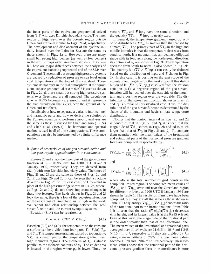
Noting that the contour interval in Figs. 2b and 2dis double of that in Figs. 2i and 2j, it is seen that themagnitude of =f ei shown in Figs. 2b and 2d is muchlarger than that of =h i in Figs. 2i and 2j. To comparethem quantitatively, the mean values of the irrotationaland rotational parts of the horizontal pressure gradientforce are computed, respectively, by

1/22 2M N1 ]f ]fei ei|=f | 5 1 (4.2)O Oei m 1 2 1 2[ ]MN ]x ]yl51 j51 l, j l, j

and1/22 2M N1 ]h ]hi i|=h | 5 1 , (4.3)O Oi m 1 2 1 2[ ]MN ]x ]yl51 j51 l, j l, j

where MN is the total number of grid points in thecomputed limited region. The computed mean values of|=f ei|m and |=hi|m over and near the Greenland regionfor different s levels at 1200 UTC 8 January 1992 areshown in Table 1. The results of many days have beencomputed, but they are all the same as those shown inTable 1. The quantity (|=hi|m)/(|=f ei|m) denotes the ratioof the rotational part to the irrotational one. From Table1 it is seen that the ratio (|=hi|m)/(|=f ei|m) decreaseswith height, and its largest value is at the 0.995 s level.Even at this level, the magnitude of the rotational partis one order smaller than that of the irrotational one.The mean values of the irrotational and rotational partsaveraged over all s levels are 21.616 3 1024 and 1.3483 1024 m s22, respectively. If they are divided by f 0,using a mean latitude of 708N, the two mean valuesbecome 15.78 and 0.984 m s21, respectively. These twomean values show that the rotational part of the hori-zontal pressure gradient force in s coordinates is more


TABLE 1. Mean values of the irrotational and rotational parts ofthe horizontal pressure gradient force in s coordinates (unit: 1024 ms22). Computed over and near the Greenland region at 1200 UTC 8January 1992.

s-levels | =sei |m | =hi |m | =hi |m/| =sei |m

0.025 37.7305 1.2405 0.032880.075 25.5285 0.9953 0.037810.105 23.3589 0.9123 0.039060.125 22.6787 0.9270 0.040870.170 22.5612 0.9819 0.043520.240 23.6746 1.2636 0.052930.325 25.5012 0.9785 0.038370.430 24.1709 1.1585 0.047930.550 21.6993 1.4696 0.067730.670 19.6732 1.3755 0.069920.775 18.0731 1.2353 0.068350.855 16.5819 1.3721 0.082750.915 15.8623 1.6356 0.103110.955 15.8803 1.8660 0.117500.980 16.1932 2.0390 0.125910.995 16.4882 2.1470 0.13021Mean value 21.6160 1.3480 0.06326

than one order of magnitude smaller than its irrotationalpart. Thus, the geostrophic approximation (3.12) can beapproximately rewritten as

f k 3 V ù 2=f e. (4.4)

The irrotational and rotational parts of the horizontalpressure gradient force can be independent of each other.The geostrophic approximation for the irrotational pres-sure gradient force (or the rotational wind) is expressedby (3.17). Figures 2l and 2m are the inner part of thestreamfunction at the s 5 0.995 level for 1200 UTC 8and 9 January 1992, respectively. They are derived from(2.6) based on the wind field of the ECMWF analysis.Comparing Figs. 2l and 2m with Figs. 2b and 2d, re-spectively, it is seen that they are very similar over theregion including Greenland. Thus, from qualitative in-spection, the geostrophic relation for the rotational wind(3.17) is approximately satisfied at s 5 0.995 overGreenland.

The geostrophic approximation for the rotationalpressure gradient force (or the divergent wind) is ex-pressed by

12 2D 5 ¹ x ù ¹ h. (4.5)

f0

Equation (4.5) can be solved with zero Dirichlet bound-ary value in a limited region; its solution becomes

f 0hi . xi. (4.6)

Figures 2n and 2o are the inner part of the velocitypotential derived from (2.6) based on the wind field atthe s 5 0.995 level for 1200 UTC 8 and 9 January1992, respectively. From Fig. 2n, it is seen that thevelocity potential is very small over the Greenland re-gion. When the cyclone develops over the east coast ofGreenland at 1200 UTC 9 January 1992, an area of high

velocity potential also develops over that region at thes 5 0.995 level as shown in Fig. 2o. A center of highvelocity potential corresponds to wind convergence.Comparing Figs. 2n and 2o with Figs. 2l and 2m, re-spectively, we cannot find any relation satisfying ap-proximation (4.6). In Fig. 2o, there is a region of highvelocity potential over the east coast of Greenland. Ac-cording to (4.6), the geo-streamfunction should alsohave a high value region over that area. However, thecomputed geo-streamfunction shown in Fig. 2m is a lowcenter over that region. It is seen that the approximation(4.6) between the inner parts of the geo-streamfunctionand divergent wind does not exist in the real atmosphere.

The geostrophic approximation (3.11) is the first-or-der approximation of (3.10), which means that the mag-nitudes of the last term on the left-hand side of (3.10)and first two terms on its right-hand side are one orderlarger than that of the other terms in the equation. Ifthe horizontal pressure gradient force is separated intoits irrotational and rotational parts, and the magnitudeof the rotational part is one order smaller than that ofthe irrotational part, the magnitude of the terms in(3.10), which correspond to the two terms in (4.6), isno longer one order larger than that of the other termsin (3.10). Thus, approximation (4.6) does not exist. Thegeostrophic approximation in s coordinates can be ex-pressed only by (3.17) and (4.4) but not by (4.6).

The above computed example further shows that, be-cause the rotational part of the horizontal pressure gra-dient force is so small, it need not be considered in thegeostrophic approximation and synoptic analysis.

The purpose of this paper is to propose a new variablef e that is used in s coordinates in the same manner asf (x, y, p, t) is used in p coordinates, rather than justcalculating the geostrophic wind over mountain regions.The equivalent geopotential f e can also be used in trop-ical and equatorial regions. However, the geostrophicapproximation is a useful tool for geopotential analysison isobaric surfaces. The geostrophic approximationshown by (4.4) and (3.17) for f e is the same as thatfor f (x, y, p, t), thus it must be very useful for equivalentgeopotential analysis on constant s surfaces.

c. Systems over the Tibetan Plateau analyzed by theinner part of the equivalent isobaric geopotentialat s 5 0.995

Because weather systems over the Tibetan Plateau arevery difficult to identify on lower-tropospheric synopticanalyses (e.g., SLP, 850 hPa, and 700 hPa), the equiv-alent isobaric geopotential analysis on the constant ssurface is especially useful for this plateau region. Fig-ure 1a shows the topography over east Asia, in whichthe largest mountain is the huge Tibetan Plateau, whosemaximum height is greater than 5000 m. The Altai-Sayan Mountains, with a height of about 2200 m, arelocated to the southwest of Lake Baikal. The height andhorizontal scale of the Altai-Sayan Mountains are com-


FIG. 3. (a) The inner part of the equivalent isobaric geopotential height at 1200 UTC 14 April 1988 at s 5 0.995 (in 10 m2 s22 andcontour interval: 30 3 10 m2 s22; the heavy dashed line shows the sketch of the Tibetan Plateau and the fronts have also been presented).(b) Same as (a) except for 0000 UTC 15 April 1988. (c) Same as (a) except for 1200 UTC 15 April 1988. (d) Same as (a) except for 0000UTC 16 April 1988. (e) SLP at 1200 UTC 14 April 1988 (3-hPa isobar spacing). (f ) Same as (e) except for 0000 UTC 15 April 1988. (g)Same as (e) except for 1200 UTC 15 April 1988. (h) Same as (e) except for 0000 UTC 16 April 1988. (i) The inner part of the streamfunctionat 1200 UTC 14 April 1988 at the level s 5 0.995 (in 105 m2 s21 and contour interval: 30 3 105 m2 s21). (j) A schematic diagram for theearly stage of an SW vortex formed on the eastern flank of the Tibetan Plateau.

parable to those of the Alps. In the lee of the Altai-Sayan Mountains, lee cyclogenesis often occurs. In theanalysis of the constant s surface, 16 s levels shownabove are used. The mesh size of the limited region is61 3 51 and the grid spacing is 170 km.

The inner part of the equivalent isobaric geopotentialat s 5 0.995 for 1200 UTC 14 April 1988 is shown inFig. 3a. It is seen from Fig. 3a that a mature cyclonemoves eastward to the north of Lake Baikal, which maybe referred to as the parent cyclone according to Palmenand Newton (1969). A front trailing from the cycloneis oriented from northeast to southwest with a cold high

behind. The inner part of the equivalent geopotential ats 5 0.995 for 0000 and 1200 UTC 15 April and 0000UTC 16 April 1988 is presented in Figs. 3b–d, respec-tively. In Fig. 3b, a pressure ridge is formed on thewindward side of Altai-Sayan when the front movingeastward is retarded by mountains. At the same time,the equivalent isobaric geopotential on the lee side ofthe mountains starts to fall and a pressure trough appearsover the Mongolian Plateau ahead of the front. Twelvehours later as shown in Fig. 3c, a lee cyclone has formedwith the central height of about 275.9 m. The value ofthe inner part of the equivalent isobaric geopotential


FIG. 3 (Continued)


FIG. 4. (a) The geopotential height [solid line at 80 gpm (geopotential meter) spacing], wind (arrows with scale in m s21 at bottom), andtemperature (dashed line in 4 K increments) at the 850-hPa level at 0000 UTC 15 April 1988; the heavy dashed line shows the outline of

height is relative, corresponding to zero value at theboundary. At 0000 UTC 16 April as shown in Fig. 3d,this cyclone has grown to its mature state. However, thecentral value does not decrease, but rather increases andthen stays unchanged at 270 m. The lee cyclone sep-arates from the parent cyclone as the latter moves awayfrom the limited region.

The SLP analyses at 1200 UTC 14 April, 0000 and1200 UTC 15 April, and 0000 UTC 16 April 1988 arepresented in Figs. 3e–h, respectively. These analyses aredirectly based on ECMWF analysis and do not separatethe inner and harmonic parts. Thus, only the inner regionof Figs. 3e–h can be compared with Figs. 3a–d. Theheavy dashed line is the outline of the Tibetan Plateau.These analyses are very similar to Figs. 3a–d, respec-

tively, in the region far away from the Tibetan Plateau.They have a similar depiction of the lee cyclone de-velopment. However, over the Tibetan Plateau, the an-alyses in Figs. 3e–h are different from those in Figs.3a–d, respectively. In Figs. 3e–h over the Tibetan Pla-teau, there are many anomalous high and low centersin these SLP maps. These high and low systems arecaused by reduction of pressure to sea level using thedata from upper-atmospheric levels. Some of them looklike the topography, and there is no weather significanceattached to these anomalous systems. However, if theequivalent isobaric geopotential at s 5 0.995 is usedas shown in Figs. 3a–d, these artificial systems over theTibetan Plateau are all removed.

From 1200 UTC 14 April (Fig. 3a) to 0000 16 April


FIG. 4 (Continued) the Tibetan Plateau. (b) Same as (a) except for the 700-hPa level. (c) Same as (a) except for 1200 UTC 15 April 1988.(d) Same as (c) except for the 700-hPa level. (e) Same as (a) except for 0000 UTC 16 April 1988. (f ) Same as (e) except for the 700-hPalevel.

1988 (Fig. 3d), the anticyclone behind the lee cyclonemoves toward the southeast, and it causes cold air toaffect the eastern part of the Tibetan Plateau. The coldair is separated from the major anticyclone to form asecondary high over the Tibetan Plateau at 0000 16April 1988. This secondary high can be seen clearly inFig. 3d over the plateau, but cannot be identified in Fig.3h.

Figure 3i is the inner part of the streamfunction de-rived from the wind field at s 5 0.995 level for 1200UTC 14 April 1988. Comparing Fig. 3i with Fig. 3a, itis seen that they are similar over the region includingthe Tibetan Plateau. The geostrophic relation for therotational wind on the constant s surface (3.17) is ap-proximately satisfied at the s 5 0.995 level over theTibetan Plateau, although this approximation is not asgood as that in high latitudes, such as the approximationbetween Figs. 2b and 2l and that between Figs. 2d and2m.

d. A southwest vortex analyzed by the equivalentisobaric geopotential at s 5 0.825 and 0.735 nearthe Tibetan Plateau

Over the eastern flank of the Tibetan Plateau, a lowpressure system called a southwest (SW) vortex (due toits origin in southwestern China) is frequently observedbetween the 700- and 850-hPa levels, and a schematicthree-dimensional diagram for the early stage of an SWvortex is shown in Fig. 3j. The SW vortices are cyclonicand their horizontal scale is several hundred kilometers.It is not clear what is the major factor causing these lowvortices at their early stage. The vortices normally form

in regions with horizontally uniform temperature andaway from major baroclinic zones. Some remain in thisenvironment for several days and then decay locally.Others are affected by cold fronts arriving from the northalong the eastern edge of the Tibetan Plateau. If thevortices are affected by cold fronts, they move awayfrom their place of origin, develop further, and produceprecipitation in the downstream region (Kuo et al. 1986;Ma and Bosart 1987; Wang et al. 1993). This is animportant type of rain-producing system in China. It iseasy to see from Fig. 3j that the early stage of an SWvortex is very difficult to identify on the isobaric ana-lyses at the 850- and 700-hPa levels. Sometimes we canfind only half of the wind circulation on these isobaricsurfaces. However, the equivalent isobaric geopotentialanalysis is very useful for identifying the early stage ofSW vortices.

We compare the equivalent isobaric geopotential an-alyzed at the levels s 5 0.825 and 0.735 with the geo-potential, temperature, and wind analyses at the 850-and 700-hPa levels. The examples are the same as thosestudied in section 4c. The geopotential, temperature, andwind fields at the 850- and 700-hPa levels from 0000UTC 15 April to 0000 UTC 16 April 1988 are shownin Figs. 4a–4f, respectively. These figures are analyzedfrom the data of ECMWF. Because the 850- and 700-hPa levels over the Tibetan Plateau are below the earth’ssurface, the data at these levels are all extrapolated fromthe upper troposphere.

The inner part of the equivalent geopotential at s 50.825 and 0.735 levels for 0000 and 1200 UTC 15 Apriland 0000 UTC 16 April 1988 is presented in Figs. 5a–


→

FIG. 5. (a) The inner part of the equivalent isobaric geopotential height at 0000 UTC 15 April 1988 at s 5 0.825 (in 10 m2 s22 and contourinterval: 30 3 10 m2 s22; the heavy dashed line shows the sketch of the Tibetan Plateau). (b) Same as (a) except for s 5 0.735. (c) Sameas (a) except for 1200 UTC 15 April 1988. (d) Same as (c) except for s 5 0.735. (e) Same as (a) except for 0000 UTC 16 April 1988. (f )Same as (e) except for s 5 0.735.

f, respectively. In Figs. 5a and 5b, there is a high geo-potential region over the major part of the Tibetan Pla-teau, but a weak low value region is located over itseastern flank and the Sichuan Basin. In Figs. 5c and 5d,in addition to a low geopotential system developing overthe Mongolian Plateau associated with lee cyclogenesis,there is an SW low vortex present over the eastern flankof the Tibetan Plateau and the Sichuan Basin. However,as shown in Figs. 4c and 4d, this SW low vortex isdifficult to identify on the corresponding 850- and 700-hPa analyses.

In Figs. 5e and 5f, the troughs associated with the leecyclone at s 5 0.825 and 0.735 levels are further de-veloped, and their southern parts affect the SW low. TheSW low is influenced by the cold air arriving from thenorth along the eastern edge of the Tibetan Plateau, andit becomes the shortwave trough shown in Figs. 5e and5f. In this situation, the shortwave trough often moveseastward and develops further. Its further developmentis away from the Tibetan Plateau, and it will be thesame as the analyses in p coordinates and is not dis-cussed here.

The early stages of an SW low can be identified bythe equivalent isobaric geopotential analysis at s 50.825 and 0.735 as shown more clearly by Figs. 5c and5d. On the other hand, the secondary high over theTibetan Plateau shown in Fig. 3d can also be seen inthe analyses for the same time at s 5 0.825 as shownin Fig. 5e. This secondary high is associated with arelatively cold area in the temperature field over theTibetan Plateau as revealed by Figs. 4e and 4f.

It is seen from the above that equivalent isobaric geo-potential analysis at s 5 0.825 and 0.735 levels canidentify weather systems more clearly than the conven-tional analyses at the 850- and 700-hPa levels over andnear the Tibetan Plateau.

5. Application of the equivalent isobaricgeopotential to the inner part equations ofstreamfunction and velocity potential

a. Application of the equivalent geopotential to thevorticity and divergence equations

It is assumed that

f 5 f 0 1 f 9, and m2 5 1 (m2)9,2m0 (5.1)

where f 0 and are the averaged values of the Coriolis2m0

parameter and m2, respectively, over the integration re-gion, and f 9 and (m2)9 are their deviations, respectively.The temperature is divided into a stationary portion andits deviation, and is expressed by

T 5 T (x, y, s) 1 T9(x, y, s, t)0

5 T (x, y, s) 1 (T(x, y, s, t) 2 T (x, y, s)). (5.2)0 0

If the model is used for a diagnostic study or a shorttime integration, the stationary portion is assumed to bethe initial value as

T0(x, y, s) 5 T(x, y, s, t0). (5.3)

The vorticity and divergence equation are derivedfrom (3.10) and written in the form

]z25 2 f d 1 m V (5.4)0 adv]t

]d2 2 25 f z 2 m ¹ f 2 m = · (RT (x, y, s)= lnp )0 0 *]t

2 2 21m D 2 m ¹ E, (5.5)adv

where

] y ] u2z 5 k · = 3 V 5 m 2 ,1 2 1 2[ ]]x m ]y m

] u ] y2d 5 = · V 5 m 11 2 1 2[ ]]x m ]y m

u ]( f9 1 z) y ]( f9 1 z) dV 5 2 1 2 ( f9 1 z)adv 21 2m ]x m ]y m

]T (x, y, s) ] lnp ]T (x, y, s) ] lnp0 0* *1 R 21 2]x ]y ]y ]x

]F ]Fy u1 2 , (5.6)]x ]y

y ]( f9 1 z) u ]( f9 1 z) zD 5 2 1 ( f9 1 z)adv 2m ]x m ]y m

2 2]F ]F u 1 yu y1 1 , E 5 . (5.7)]x ]y 2

Here

]u/m ] lnp Px*F 5 2s 2 RT9(x, y, s, t) 1 ,u ]s ]x m

P]y /m ] lnp y*F 5 2s 2 RT9(x, y, s, t) 1 . (5.8)y ]s ]y m

The main parts of Vadv and Dadv on the right-hand sideof (5.6) and (5.7) are advection, so that Vadv and Dadv

are briefly termed the generalized vorticity and diver-


gence advection, respectively. Using the definition sim-ilar to (3.13), (5.6) can be written as

u ]( f9 1 z) y ]( f9 1 z)V 5 2 1adv 1 2m ]x m ]y

d ]F ]Fy u22 ( f9 1 z) 2 ¹ h 1 2 . (5.69)2m ]x ]y

Based on Figs. 2i and 2j, it is seen from (5.6a) that theeffect of the rotational part of the horizontal pressuregradient force increases anticyclonic and cyclonic vor-ticity in the east and west flanks of mountains, respec-tively, in the middle and high latitudes of the NorthernHemisphere. Using (2.6), (5.4) and (5.5) in a limitedregion are rewritten as

2]¹ ci 25 2 f ¹ x 1 V (5.9)0 i adv]t2]¹ xi 2 25 f ¹ c 2 ¹ f 2 = · (RT (x, y, s)= lnp )0 i i 0 *]t

22 ¹ E 1 D . (5.10)i adv

In s coordinates, the thermodynamic, continuity, andhydrostatic equations are expressed by

]T ]T RT5 2V · =T 2 s 1 v

]t ]s C Pp

11 [L(C 2 E ) 1 Q ] (5.11)TCp

] lnp ]s* 5 V · = lnp 2 = · V 2 (5.12)*]t ]s

]f RT5 2 , (5.13)

]s s

where C and E are the rate of condensation and evap-oration per unit mass, respectively, QT is the heatingrate per unit mass due to the turbulent transfer and ra-diation.

b. The inner part equations of the streamfunction andvelocity potential

Let us introduce two variables, cadv,i and xadv,i, whichsatisfy the following equations:

¹2cadv,i 5 Vadv, ¹2xadv,i 5 Dadv (5.14)

with the homogeneous Dirichlet boundary values. Thevariables cadv,i and xadv,i are referred to as the variationrates caused primarily by advection for the inner partsof the streamfunction and velocity potential, respec-tively.

If the integral operator ¹22, shown in the appendix,is used for the solution of the Poisson equation withzero Dirichlet boundary value, then the solutions of(5.14) are expressed by

cadv,i 5 ¹22Vadv, xadv,i 5 ¹22Dadv. (5.15)

For a synoptic analysis or a diagnostic study, T9 van-ishes in (5.2) because only the time at t0 is considered.Thus, the inner part of the equivalent isobaric geopo-tential height (3.5) can be further rewritten in the form

] ] lnp22 *f 5 f 1 ¹ RT (x, y, s)ei i 01 2[]x ]x

] ] lnp*1 RT (x, y, s) , (5.16)01 2]]y ]y

where T0(x, y, s) satisfies (5.3).In a general dynamical study, such as short-range

weather prediction, T9 does not vanish. Equation (5.16)can be considered a new definition for the inner part ofthe equivalent isobaric geopotential in the general case.Comparing (5.2) with (3.8) and (3.9), T9(x, y, s, t) cor-responds to Tsy, the temperature caused by the transientsynoptic disturbances. The stationary portion, T0(x, y,s), corresponds to the sum of T0(s), Tor, and Tcl . Asmentioned in section 3, the temperature caused by to-pography, Tor, is a major part of T(x, y, s, t) over highmountain regions, and it makes an important contri-bution to f ei. Many spectral models and CBB use thegeneralized geopotential derived based on T0(s) only.Over high mountain regions, the equivalent geopotentialderived from (5.16) is quite different from the gener-alized geopotential derived based only on T0(s).

Utilizing (5.15) and (5.16), (5.9) and (5.10) can besolved with zero Dirichlet boundary values, and theirsolutions become

]ci 1 f x 5 c (5.17)0 i adv,i]t

]xi 1 f 2 f c 5 x 2 E . (5.18)ei 0 i adv,i i]t

Equations (5.17) and (5.18) are the inner part equationsof streamfunction and velocity potential, respectively.

During computations with the primitive equations ins coordinates, the absolute values of the first two termson the right-hand side of (3.10) are very large near highmountains. The horizontal pressure gradient force isonly a small difference between these two large terms,and its computational errors become very large nearsteep slopes. A number of authors (e.g., Corby et al.1972; Gary 1973; Sundqvist 1976; Nakamura 1978;Mesinger et al. 1988) examined how these errors canbe reduced during computations with primitive equationmodels. If the horizontal pressure gradient force is sep-arated into its irrotational and rotational parts, the firsttwo terms on the right-hand side of (3.10) are replacedby the two terms on the right-hand side of (3.12). Inthis case, the computational problem in primitive equa-tion models is automatically eliminated.


FIG. 6. The vertical distribution of the variables.

6. The inner part equation of the equivalentisobaric geopotential height

a. The vertical difference form of the continuityequation and hydrostatic equation

To develop the equivalent isobaric geopotential equa-tion, the vertical difference forms of the continuity, hy-drostatic, and thermodynamic equations need to be used.The vertical distribution of variables is shown in Fig.6. Based on (2.24) of CBB, the vertical difference formof the continuity equation (5.12) can be rewritten as

] lnp2* 1 m PD↓ 5 P , (6.1)0 adv

]t

where Padv is dominated by the surface pressure advec-tion and it is expressed by

N ] lnp ] lnp2 * *P 5 2m U 1 V DsOadv j j j1 2]x ]yj51

22 (m )9PD↓, (6.2)

and D↓ and P indicate the column vector and row vec-tor, respectively, as

TD↓ 5 (D , . . . , D , . . . , D ) ,1 k N

P 5 (Ds , . . . , Ds , . . . , Ds ), (6.3)1 k N

where (. . .)T is for transpose. As shown in CBB, boththe sigma vertical velocity, , and local pressuresk11/2

tendency, (] lnp*/]t), can be divided into their divergentpart and surface pressure advective part, and the verticaldifference forms of these two parts are expressed by

N k

s 5 s d Ds 2 d Ds ,O Odiv,k11/2 k11/2 j j j jj51 j51

N

s 5 s V · = lnp DsOspa,k11/2 k11/2 j j*j51

k

2 V · = lnp Ds (6.4)O j j*j51

N] lnp* 5 2 d Ds ,O j j1 2]t j51div

N] lnp* 5 2 V · lnp Ds . (6.5)O j j1 2 *]t j51spa

Based on (A.17) of CBB, the pressure vertical ve-locity is written by

v ] lnp ] lnp2 * *↓ 5 m (I 2 C) U↓ 1 V↓1 2 1 2p ]x ]y

22 m CD↓, (6.6)

where I is an unit matrix, and C is a lower-triangularmatrix denoted by (A.15) of CBB.

Based on (A.28) of CBB, the finite difference formof the hydrostatic equation is expressed by

f↓ 5 f*↓ 1 RBT↓, (6.7)

where matrix B is an upper-triangular matrix expressedby (A.29) of CBB, and f*↓ 5 f*I. Here f* 5 gH*,and H* is the height of the earth’s surface.

b. The vertical difference form of the thermodynamicequation

The thermodynamic equation (5.11) can be rewritten as

2k]T9 u ]T y ]T ]T2 k5 2m 1 2 s s[ ]]t m ]x m ]y ]s

1 kT ln p 1 P , (6.8)T*

where k 5 R/Cp and PT 5 (L(C 2 E) 1 QT)/Cp. Thestationary portion of temperature can further be sepa-rated into two parts:

T (x, y, s) 5 T (s) 1 T9(x, y, s)0 00 0

5 T (s) 1 (T (x, y, s) 2 T (s)), (6.9)00 0 00

where T00(s) is the averaged value of T0 over the con-stant s surface, and is its deviation.T90

Based on the separations (6.4) and (6.5), Eq. (6.8)can be rewritten as

2k]T9 ]T s ] lnp00k *5 2s s 1 kTdiv 001 2]t ]s ]tdiv

1 T 1 P , (6.10)adv T

where


2ku ]T y ]T ](T9 1 T9)s02 kT 5 2m 1 2 s sadv div[ ]m ]x m ]y ]s

2k] lnp ]Tsk*1 k(T9 1 T9) 2 s s0 spa1 2]t ]s

div

] lnp u ] lnp y ] lnp2* * *1 kT 1 kTm 1 .1 2 [ ]]t m ]x m ]y

spa

(6.11)

Substituting (6.4) and (6.5) into (6.10) and (6.11),similar to (A.33) of CBB, the vertical difference formof (6.10) can be written as

N]T9k 25 T 2 m F D 1 P , (6.12)Oadv,k k,l l T,k]t l51

where Tadv,k is the vertical difference form of (6.11), andthe elements of matrix F are defined as

ks k 2k 2kF 5 [(T s 2 T s )(s Ds 2 e )k,l 00,k11 k11 00,k k k11/2 l 12Dsk

2k 2k1 (T s 2 T s )(s Ds 2 e )]00,k k 00,k21 k21 k21/2 l 2

1 kT Ds . (6.13)00,k l

Here

0, if l . k,« 51 5Ds , if l # k,l

0, if l . k 2 1,« 5 (6.14)2 5Ds , if l # k 2 1.l

c. The equation of the inner part of the equivalentisobaric geopotential height

Substituting the inner part of the hydrostatic equation(6.7) into (5.16), the vertical difference form of (5.16)is expressed by

f ↓ 5 f ↓ 1 RBT ↓ei i i*

] ] lnp ] ] lnp22 * *1 ¹ RT ↓ 1 RT ↓ .0 01 2 1 2[ ]]x ]x ]y ]y

(6.15)

Taking the partial derivative of (6.15) with respect to t,and utilizing (6.9), we have

]f ↓ ]T9↓ ] lnpei i i*5 RB 1 RT ↓00]t ]t ]t

] ] ] lnp22 *1 ¹ RT9↓01 2[]x ]x ]t

] ] ] lnp*1 RT9↓ . (6.16)01 2]]y ]y ]t

Utilizing (2.18), the inner part equations of (6.1) and(6.12) can be derived. Substituting (6.1) and the derivedinner part equations of (6.1) and (6.12) into (6.16), then(6.16) becomes

]f ↓ei 21 m AD ↓ 5 F ↓, (6.17)0 i e,had,i]t

where matrix A is

A 5 R(BF 1 T00↓ P) (6.18)

and Fe,had,i↓ denotes the variation rate of the inner partof the equivalent isobaric geopotential caused by theadvection and heating, and it is expressed by

F ↓ 5 RBT ↓ 1 RT ↓P 1 RBP ↓e,had,i adv,i 00 adv,i T,i

2] ](P 2 m PD↓)adv 0221 ¹ RT9↓01 2[]x ]x

2] ](P 2 m PD↓)adv 01 RT9↓ .01 2]]y ]y

(6.19)

Based on

D↓ 5 Di↓ 1 Dh↓ (6.20)

and (2.6), the vertical difference form of the inner partequation of the equivalent isobaric geopotential (6.17)is rewritten in the form

]f ↓ei 2 2 21 m A¹ x ↓ 5 F ↓ 1 m AD ↓. (6.21)0 i e,had,i 0 h]t

Equations (5.17), (5.18), and (6.21) are the basic equa-tions for application of the equivalent isobaric geopo-tential to numerical prediction, initialization, and otherdynamic studies. As a simple example, these equationsare used to derive a generalized v equation in s co-ordinates presented in the next section.

7. A velocity potential form of the generalized vequation in the balanced ageostrophicapproximation and its solution

a. An ageostrophic geopotential height ins coordinates

Utilizing the wind patitioning into the streamfunctionand velocity potential, the inner part of the equivalentisobaric geopotential can be separated into a geostrophicpart and an ageostrophic part as

f ei 5 f ei,g 1 f ei,a, (7.1)

where the geostrophic part based on (3.17) is definedby

f ei,g 5 f 0ci, (7.2)

and the ageostrophic part is defined by the differencebetween the equivalent geopotential and its geostrophicpart, and expressed by


f ei,a 5 f ei 2 f ei,g 5 f ei 2 f 0ci. (7.3)

In definitions (7.2) and (7.3), f 0 is not present in thedenominator. In the equatorial region where f 0 ap-proaches zero, the geostrophic part becomes zero, thatis, f ei,g 5 0; and the ageostrophic part (7.3) becomesthe equivalent geopotential, that is, f ei,a 5 f ei . Thus,definitions (7.2) and (7.3) are different from the tradi-tional definitions of the geostrophic and ageostrophicwinds, and they can be used all over the globe includingthe equatorial region.

The vertical difference form of the inner part equa-tions for streamfunction and velocity potential (5.17)and (5.18) can be rewritten, respectively, as

]c ↓i 1 f x ↓ 5 c ↓, (7.4)0 i adv,i]t

]x ↓i 1 f ↓ 5 x ↓ 2 E ↓. (7.5)ei,a adv,i i]t

b. The equation of the inner part of the ageostrophicgeopotential height

From (7.4) and (6.21), the equation of the inner partof the ageostrophic geopotential can be derived and itis denoted by

]f ↓ei,a 2 2 2 21 m A¹ x ↓ 2 f x ↓ 5 F ↓ 1 m AD ↓,0 i 0 i e,had,ia 0 h]t(7.6)

where

Fe,had,ia↓ 5 Fe,had,i↓ 2 f 0cadv,i↓ (7.7)

is referred to as the variation rate of the ageostrophicgeopotential caused by advection and heating.

Equations (7.4), (7.5), and (7.6) are the basic equa-tions in a limited region for three variables: the innerparts of the streamfunction, velocity potential, andageostrophic geopotential.

c. A velocity potential form of the generalized vequation in s coordinates with the balancedageostrophic approximation

Recently, an approximation where the tendencies ofthe ageostrophic geopotential and velocity potential in(7.6) and (7.5) vanish has been used in an initializationby Chen et al. (1996) and referred to as the balancedageostrophic approximation. They proved that the bal-anced ageostrophic approximation is much more ac-curate than the quasigeostrophic approximation.

If the tendency of the ageostrophic geopotential isneglected in (7.6), (7.6) becomes

A¹2x i↓ 2 xi↓ 5 Fe,had,ia↓ 1 ADh↓. (7.8)2 2 2m f m0 0 0

Equation (7.8) is a velocity potential form of the gen-eralized v equation in s coordinates with the balancedageostrophic approximation. The advection terms com-

puted by the ageostrophic wind in (7.8) are the same asthose in the generalized v equation in p coordinates(Pauley and Nieman 1992), but the effect of orographyon the vertical motion is better described by (7.8).

If the variation rate of the ageostrophic geopotentialcaused by advection and diabatic heating is computedfrom the geostrophic wind, and it is expressed byFe,had,ia,g↓, then (7.8) becomes

A¹2x i↓ 2 xi↓ 5 Fe,had,ia,g↓ 1 ADh↓. (7.9)2 2 2m f m0 0 0

Equation (7.9) is a velocity potential form of the qua-sigeostrophic v equation in s coordinates.

d. The solution of the velocity potential form of thegeneralized v equation

Equation (7.8) can easily be solved by transformingit into vertical mode space. For this purpose, we intro-duce a matrix, E, in order that the following relation issatisfied

E21AE 5 G 5 diag(gh1, gh2, . . . , ghN). (7.10)

The matrix E is derived from the eigenvectors of thematrix A, and these eigenvectors are denoted by Ej↓, j5 1, . . . , N. The matrix E is an eigenvector matrix witheach column representing an eigenvector Ej↓. The ma-trix E21 is the inverse of the matrix E. The matrix G isa diagonal matrix with the diagonal elements given bythe N eigenvalues, (gh1, gh2, . . . , ghN), of the matrixA.

The transformation of velocity potential between thevertical mode and physical space is expressed by

xi*↓ 5 E21xi↓, xi↓ 5 Exi*↓. (7.11)

If Eq. (7.8) is multiplied from left by the matrix E21,then (7.8) becomes

G¹2x i*↓ 2 xi*↓ 5 Fe,had,ia*↓ 1 GDh*↓,2 2 2m f m0 0 0

(7.12)

where

Fe,had,ia*↓ 5 E21Fe,had,ia↓, Dh*↓ 5 E21Dh↓.(7.13)


1 12 2¹ x 2 x 5 (F 1 C D ),i*k i*k e,had,ia*k k h*k2 2L C0k k

k 5 1, 2, . . . , N, (7.14)

where

22m gh C0 k k2C 5 m Ïgh , and L 5 5 (7.15)k 0 k 0k 2 1 2f f0 0

are the gravity wave phase speed and radius of defor-mation of the kth vertical mode, respectively.

Because the lateral boundary value of the inner partof the velocity potential is homogeneous, the solution


of the Helmholtz equation (7.14) can be derived fromthe double sine series. Based on (A.2) and (A.3) in theappendix, the solution of (7.14) is written in the form

211 1 12x 5 2F (F 1 C D ) 1 .i*k,mn e,had,ia*k k h*k2 2 21 2[ ]C L Lk mn 0k

(7.16)

After the vertical mode of the velocity potential,xi*,mn↓, is derived, we have

xi*k 5 F21[xi*k,mn], xi↓ 5 Exi*↓. (7.17)

Based on (6.6), the pressure vertical velocity is de-termined by

v ] lnp ] lnp2 * *↓ 5 m (I 2 C) U↓ 1 V↓1 2 1 2p ]x ]y

2 22 m C¹ x ↓. (7.18)i

The horizontal divergence in (7.18) can also be com-puted directly from the observed wind, and it is referredto as a kinematic method. However, the horizontal di-vergence derived from the kinematic method is sensitiveto small errors in the observed wind. The divergencederived from (7.16) is determined from terms of similarmagnitude and is less sensitive to observational errorsthan the kinematic method; it is referred to as an v-equation method. Because the v-equation method in-volves computations of higher-order derivatives than thekinematic method, this diminishes the advantages if thecomputation of derivatives is not accurate enough. Thus,in order to reduce computational errors, a harmonic-sinespecial method (Chen and Kuo 1992a) is used here.

8. Some test results of the annual precipitationover Greenland

The computation procedure for precipitation based oncomputed vertical motion is given by Chen et al.(1997b). Only large-scale condensation is considered inthe precipitation. The computation procedure for thelarge-scale condensation and precipitation is similar tothat discussed by Arakawa and Lamb (1977). In thiscomputation procedure, the temperature variation in atime step is computed from horizontal and vertical ad-vection and adiabatic variation based on the thermo-dynamic equation (6.11) and (6.12). The specific hu-midity variation in a time step is deduced from the con-tinuity equation for specific humidity. In these equa-tions, the sigma vertical velocity, , is computedsk11/2

from (6.4), in which the horizontal divergence is ob-tained from solution (7.16). The precipitation rate isonly computed for one time step, which is 30 min, andthen it is applied to a 12-h period. The precipitation iscalculated twice per day based on the analyzed data at0000 and 1200 UTC from ECMWF. The annual pre-cipitation is derived by summing precipitation day-by-day for one year. The mesh size of the limited region

shown in Fig. 1e is 111 3 81 and the grid spacing is50 km. In the vertical, the 16 s levels are the same asused in section 4.

Of course, the above method for retrieving precipi-tation is not rigorous, but it is very simple in comparisonto a limited-area FDDA system. As we only want todetermine some basic features of the annual precipita-tion over Greenland, this simple method is used to seewhether or not precipitation is reasonably retrieved ifthe equivalent isobaric geopotential height is used in thegeneralized v equation.

The retrieved precipitation distributions for 1987 and1988 are shown in Figs. 7a and 7b, respectively. Todetermine whether the computed annual precipitationdistribution is reasonable, we compare it with the ob-served mean annual accumulation over the GreenlandIce Sheet shown in Fig. 1d. From Figs. 7a and 7b, it isseen that the maximum values of more than 100 cm yr21

are located along the southeastern coast and south-western edge of Greenland. A large area of very lowprecipitation (less than 20 cm yr21), which dominatesthe central interior region of Greenland, is also shownin Figs. 7a and 7b. Thus, the retrieved precipitationcaptures the main features. A secondary band of rela-tively high precipitation is present just along the westerncoast of Greenland from Jakobshavn to Thule, which isunderestimated in the simulation by Bromwich et al.(1993). However, the corresponding band in Fig. 1(d)near Jakobshavn is shifted slightly eastward into Green-land. Thus, this method also needs to be further en-hanced.

The annual precipitation over Greenland simulatedby the NCEP–NCAR Reanalysis for 1987 and 1988 isshown in Figs. 7c and 7d, respectively. It can be seenthat the annual precipitation pattern over Greenland foran individual year shown in Figs. 7c or 7d is very similarto that of the mean annual precipitation for 1982–94 inFig. 1c. A wave train pattern extending southeastward,caused by the steep slopes on the southeast coast ofGreenland, is also found in the annual precipitation inFigs. 7c and 7d for 1987 and 1988, but does not occurin Figs. 7a and 7b.

Comparing Figs. 7c and 7d with Figs. 1d and 7a and7b, it can be seen that the precipitation amounts fromthe reanalysis are about twice those observed in Fig. 1dand those retrieved in Figs. 7a and 7b. There are highprecipitation areas in the central region of Greenlandwith maxima of 111 and 101 cm yr21 in Figs. 7c and7d, respectively. They are much larger than the observedamount and the retrieved values in Figs. 7a and 7b. Theshortcomings in the mean precipitation reanalysis overGreenland shown by Fig. 1c are also present in Figs.7c and 7d.

It is seen from the above that the precipitation dis-tributions over Greenland retrieved for 1987 and 1988by the above simple method are superior to those ob-tained by NCEP–NCAR Reanalysis. This simple meth-od has been used to retrieve precipitation over Green-


FIG. 7. (a) The retrieved annual precipitation for 1987 in cm with a contour interval of 20 cm, but 10 cm if smaller than 40, and 30 cmif larger than 100. (b) Same as (a) but for 1988. (c) Annual precipitation for 1987 computed by the NCEP–NCAR Reanalysis based on aT62 model. The contour interval is 25 cm. (d) Same as (c) but for 1988.

land with reasonable accuracy, and the retrieved resultshave been used to study the basic features of the pre-cipitation over Greenland (Chen et al. 1997b).

9. Conclusions

Based on the studies shown in the above sections, thefollowing conclusions can be reached.

1) A variable f e(x, y, s, t) whose horizontal gradient2=f e on the constant s surface is equal to the irro-tational part of the horizontal pressure gradient force ins coordinates is referred to as the equivalent isobaricgeopotential height. It plays the same role in s coor-dinates as the geopotential f (x, y, p, t) does in p co-

ordinates. The analytic expression for the inner part ofthe equivalent isobaric geopotential is given by (3.5),and it is also shown by (5.16) if T0(x, y, s) is equal tothe initial value. The horizontal pressure gradient forcein s coordinates can be separated into its irrotationaland rotational parts, but the magnitude of the rotationalpart is one order smaller than that of the irrotationalpart even over high mountain regions.

2) To enable the streamfunction and velocity potentialin a limited region to be used in the same way as thestreamfunction and velocity potential on the globe and toavoid nonuniqueness, it is necessary to use the inner partsof the streamfunction and velocity potential instead of thestreamfunction and velocity potential themselves.


A horizontal vector in a limited region can be sep-arated into its internal nondivergent, internal irrotation-al, and external components as shown by (2.12). Theinner part analysis uses the inner parts of the stream-function and velocity potential and other inner part var-iables to describe motion systems in a limited region.

3) It is very difficult to use single elevation or pres-sure surface to track systems across a mountain regionat ‘‘ground’’ level. Equivalent isobaric geopotentialanalysis on the constant s surface can be used to solvethis problem. For example, if the equivalent isobaricgeopotential is used at s 5 0.995 over Greenland asshown in Figs. 2a–d, the small but strong high pressuresystems caused by pressure reduction to sea level usinglower temperatures at the top of the Greenland Ice Sheetare removed and the circulation becomes very smooth.The geostrophic relation (3.17) between the equivalentgeopotential and streamfunction on the constant s sur-face is approximately satisfied at s 5 0.995.

4) Because weather systems are very difficult to trackon synoptic analyses at sea level and at the 850- and700-hPa levels over the Tibetan Plateau, equivalent iso-baric geopotential analysis in s coordinates is especiallyuseful over this area. An example of equivalent geo-potential analysis at s 5 0.995 (Fig. 3d) shows that coldair separated from a major anticyclone to form a sec-ondary high over the Tibetan Plateau at 0000 UTC 16April 1988, but this secondary high is hard to see inthe SLP analysis (Fig. 3h). It is also found that the earlystage of an SW low (or vortex) is more clearly identifiedby equivalent isobaric geopotential analysis at s 50.825 and 0.735 (Figs. 5c and d) than by conventionalanalyses at the 850- and 700-hPa levels over and nearthe Tibetan Plateau. Anomalous high and low pressuresystems in the SLP analysis over the Tibetan Plateaucaused by extrapolation of the data from upper-tropo-spheric levels are all removed if the equivalent isobaricgeopotential is analyzed at s 5 0.995, as shown in Figs.3a–d.

5) The equivalent isobaric geopotential height in scoordinates can be used not only in synoptic analysis,but also in a dynamic study. Use of the equivalent iso-baric geopotential in the vorticity and divergence equa-tions and the corresponding inner part equations ofstreamfunction and velocity potential have been pre-sented in (5.17) and (5.18), respectively. The equationfor the equivalent isobaric geopotential in s coordinatesis given by (6.21). Equations (5.17), (5.18), and (6.21)are the basic equations for application of the equivalentisobaric geopotential to numerical prediction, initiali-zation, and other dynamic studies. As an example, Eqs.(5.17), (5.18), and (6.21) are used to derive a velocitypotential form of the generalized v equation in s co-ordinates with the balanced ageostrophic approxima-tion. This equation can easily be solved by the doublesine series and its solution is shown by (7.16). Themethod to compute vertical motion from (7.16), (7.17),

and (7.18) is referred to as the v equation method in scoordinates.

6) The vertical motion over some high mountain re-gions, such as Greenland, can be computed by this vequation method. Some test results of precipitation overGreenland retrieved by this v equation method showthat the precipitation distributions for 1987 and 1988are in good agreement with the observed annual accu-mulation distribution over the Greenland Ice Sheet, andthey are superior to the precipitation distribution derivedfrom the NCEP–NCAR Reanalysis. The computed pre-cipitation also shows that a secondary band of relativelyhigh precipitation is present along the western coast ofGreenland. The major shortcoming in the simulation byBromwich et al. (1993) is corrected. Thus, the v-equa-tion method in s coordinates is very useful for retrievingthe basic features of precipitation over Greenland.

Acknowledgments. We would like to thank the editor,Prof. Frederick Sanders, and two anonymous reviewersfor their valuable comments. Special thanks go to Lesh-eng Bai for performing some of the computations andproducing some of the figures. This research was spon-sored by NASA Grant NAGW-3677, Supplement 3, andby NOAA-Office of Global Programs GrantNA36GP0314-01. It was also supported by CentralWeather Bureau, Taipei, Taiwan, China, under ContractCWB84-3M-09. This is Contribution 1072 of the ByrdPolar Research Center.

APPENDIX

An Integral Operator ¹22 of the Poisson Equationwith Zero Dirichlet Boundary Value

The inner part of the streamfunction satisfies the Pois-son equation

¹2ci 5 V (A.1)

within the rectangular region [0 # x # Lx, 0 # y #Ly] with zero Dirichlet boundary value.

Let F denote a finite Fourier sine transform operatorin the two-dimensional rectangular region; that is,

F [V(x, y)] 5 Vmn

L Lx y4 mpx np y5 V(x, y) sin sin dx dy,E EL L L Lx y x y0 0

(A.2)

where V(x, y) can be an arbitrary function defined inthe rectangular region. The double Fourier sine seriesof f i are expressed by

21f (x, y) 5 F [F ]i I,mn

M N mpx np y5 F sin sin , (A.3)O O I,mn L Lm51 n51 x y

where F21 is the inverse Fourier sine transform operatorfrom wave to physical space, f i(x, y) is a function in


the rectangular region with zero boundary value, andFl,mn is the Fourier transform of f i.

The solution of (A.1) in wave space is expressed by

211C 5 2V , (A.4)I,mn mn 21 2Lmn

where Lmn is referred to as the horizontal scale of awavenumber (m, n), and it is expressed by

2 2 2 21 m p n p5 1 , (A.5)

2 2 2L L Lmn x y

and C l,mn is the Fourier transform of ci. Then, the so-lution of (A.1) in physical space is denoted by

21121c (x, y) 5 2F V . (A.6)i mn 21 2[ ]Lmn

The expression (A.6) can also be written in another form

ci 5 ¹22V (A.7)

thus,

21122 21¹ V 5 2F V , (A.8)mn 21 2[ ]Lmn

where ¹22 is referred to as an integral operator of thePoisson equation with zero Dirichlet boundary value.

REFERENCES

Alley, R. B., and Coauthors, 1993: Abrupt increase in Greenlandsnow accumulation at the end of the Younger Dryas event. Na-ture, 362, 527–529.

Arakawa, A., and V. R. Lamb, 1977: Computational design of thebasic dynamical process of the UCLA general circulation model.Methods Comput. Phys., 17, 173–265.

Bijlsma, S. J., L. M. Hafkensheid, and P. Lynch, 1986: Computationof the streamfunction and velocity potential and reconstructionof the wind field. Mon. Wea. Rev., 114, 1547–1551.

Bromwich, D. H., and F. M. Robasky, 1993: Recent precipitationvariations over the polar ice sheets. Meteor. Atmos. Phys., 51,259–274., , R. A. Keen, and J. F. Bolzan, 1993: Modeled variationsof precipitation over the Greenland Ice Sheet. J. Climate, 6,1253–1268.

Chen, Q.-S., and Y.-H. Kuo, 1992a: A harmonic-sine series expansionand its application to the partitioning and reconstruction problemin a limited area. Mon. Wea. Rev., 120, 91–112., and , 1992b: A consistency condition for the wind fieldreconstruction in a limited area and a harmonic-cosine seriesexpansion. Mon. Wea. Rev., 120, 2653–2670., , and D. H. Bromwich, 1996: A balanced ageostrophicinitialization with a fixed external wind lateral boundary valuefor limited-area models. J. Meteor. Soc. Japan., 74, 325–342., L. Bai, and D. H. Bromwich, 1997a: A harmonic-Fourier spec-tral limited-area model with an external wind lateral boundarycondition. Mon. Wea. Rev., 125, 143–167., D. H. Bromwich, and L. Bai, 1997b: Precipitation over Green-land retrieved by a dynamic method and its relation to cyclonicactivity. J. Climate, 10, 839–870.

Corby, G. A., A. Gilchrist, and R. L. Newson, 1972: A general cir-culation model of the atmosphere suitable for long period in-tegration. Quart. J. Roy. Meteor. Soc., 98, 809–832.

DiMego, G. J., and L. F. Bosart, 1982: The transformation of TropicalStorm Agnes into an extratropical cyclone. Part I: The observedfields and vertical motion computations. Mon. Wea. Rev., 110,385–411.

Gary, J. M., 1973: Estimate of truncation error in transformed co-ordinate, primitive equation atmospheric models. J. Atmos. Sci.,30, 223–233.

Harrison, L. P., 1957: Report on the problem of ‘‘reduction of pres-sure.’’ Report of the Working Group on Barometry to the WorldMeteorological Organization, Commission for Instruments andMethods of Observation (CIMO-II), 118 pp., 1970: Reduction of surface pressure to functions useful inanalysis and forecasting. Meteorological Observations and In-strumentation, Meteor. Monogr., No. 33, Amer. Meteor. Soc.,121–136.

Hawkins, H. F., and S. L. Rosenthal, 1965: On the computation ofstreamfunction from the wind field. Mon. Wea. Rev., 93, 245–252.

Higgins, R. W., K. C. Mo, and S. D. Schubert, 1996: The moisturebudget of the central United States in spring as evaluated in theNCEP/NCAR and the NASA/DAO reanalysis. Mon. Wea. Rev.,124, 939–963.

Hill, C. D., 1993: Forecast problems in the western region of theNational Weather Service: An overview. Wea. Forecasting, 8,158–165.

Hirschberg, P. A., and J. M. Fritsch, 1991: Tropopause undulationsand the development of extratropical cyclones. Part II: Diag-nostic analysis and conceptual model. Mon. Wea. Rev., 119, 518–550.

Iversen, T., and T. E. Nordeng, 1984: A hierarchy of nonlinear filteredmodels—Numerical solutions. Mon. Wea. Rev., 112, 2048–2059.

Johnsen, S. J., and Coauthors, 1992: Irregular glacial interstadialsrecorded in a new Greenland ice core. Nature, 359, 311–313.

Kalnay, E., and Coauthors, 1996: The NCEP/NCAR 40-Year Re-analysis Project. Bull. Amer. Meteor. Soc., 77, 437–471.

Knutson, T. R., and K. M. Weickmann, 1987: 30–60 day atmosphericoscillations: Composite life cycles of convection and circulationanomalies. Mon. Wea. Rev., 115, 1407–1436.

Krishnamurti, T. N., 1968a: A diagnostic balance model for studiesof weather systems of low and high latitudes. Rossby numberless than 1. Mon. Wea. Rev., 96, 197–207., 1968b: A study of a developing wave cyclone. Mon. Wea. Rev.,96, 208–217., 1985: Summer monsoon experiment—A review. Mon. Wea.Rev., 113, 1590–1626., and Y. Ramanathan, 1982: Sensitivity of monsoon onset todifferential heating. J. Atmos. Sci., 39, 1290–1306.

Kuo, Y.-H., L. Cheng, and R. A. Anthes, 1986: Mesoscale analysesof the Sichuan flood catastrophe, 11–15 July 1981. Mon. Wea.Rev., 114, 1984–2003.

Lynch, P., 1988: Deducing the wind from vorticity and divergence.Mon. Wea. Rev., 116, 86–93., 1989: Partitioning the wind in a limited domain. Mon. Wea.Rev., 117, 1492–1500.

Ma, K. Y., and L. F. Bosart, 1987: A synoptic overview of a heavyrain event in southern China. Wea. Forecasting, 2, 89–112.

Mesinger, F., Z. Janjic, S. Nickovic, D. Gavrilov, and D. G. Deaven,1988: The step mountain coordinate: Model description and per-formance for cases of Alpine lee cyclogenesis and for a case ofan Appalachian redevelopment. Mon. Wea. Rev., 116, 1493–1518.

Nakamura, H., 1978: Dynamical effects of mountains on the generalcirculation of atmosphere. Part I: Development of finite-differ-ence scheme suitable for incorporating mountains. J. Meteor.Soc. Japan, 56, 317–340.

Ohmura, A., and N. Reeh, 1991: New precipitation and accumulationmaps for Greenland. J. Glaciol., 37, 140–148.

Palmen, E., and C. W. Newton, 1969: Atmospheric Circulation Sys-tems. Academic Press, 419 pp.

Pauley, P. M., and S. J. Nieman, 1992: A comparison of quasigeo-


strophic and nonquasigeostrophic vertical motions for a model-simulated rapidly intensifying marine extratropical cyclone.Mon. Wea. Rev., 120, 1108–1134.

Phillips, N. A., 1957: A coordinate system having some special ad-vantages for numerical forecasting. J. Meteor., 14, 184–185.

Raisanen, J., 1995: Factors affecting synoptic-scale vertical motion:A statistical study using a generalized omega equation. Mon.Wea. Rev., 123, 2447–2460.

Sangster, W. E., 1960: A method of representing the horizontal pres-sure force without reduction of station pressure to sea level. J.Meteor., 17, 166–176., 1987: An improved technique for computing the horizontalpressure-gradient force at the earth’s surface. Mon. Wea. Rev.,115, 1358–1369.

Shukla, J., and K. R. Saha, 1974: Computation of non-divergentstreamfunction and irrotational velocity potential from the ob-served winds. Mon. Wea. Rev., 102, 419–425.

Shuman, F. G., 1957: On the problem of comparing station pressures

at varying elevations. Joint Numerical Weather Prediction UnitOffice Note 7, 10 pp. [Available from National Centers for En-vironmental Prediction, National Oceanic and Atmospheric Ad-ministration, 4700 Silver Hill Rd., Stop 9910, Washington, DC20233.]

Sundqvist, H., 1976: On vertical interpolation and truncation in con-nection with use of sigma models. Atmosphere, 14, 37–52.

Tarbell, T. C., T. T. Warner, and R. A. Anthes, 1981: An example ofthe initialization of the divergent wind component in a mesoscalenumerical weather prediction model. Mon. Wea. Rev., 109, 77–95.

Taylor, K. C., G. W. Lamorey, G. A. Doyle, R. B. Alley, P. M. Grootes,P. A. Mayewski, J. W. C. White, and L. K. Barlow, 1993: The‘‘flickering switch’’ of late Pleistocene climate change. Nature,361, 432–436.

Wang, W., Y.-H. Kuo, and T. T. Warner, 1993: A diabatically drivenmesoscale vortex in the lee of the Tibetan Plateau. Mon. Wea.Rev., 121, 2542–2561.

an equivalent isobaric geopotential height and its

Documents