an evaluation of accelerated drying of reclamation …
TRANSCRIPT

AN EVALUATION OF ACCELERATED DRYING OF
RECLAMATION SOIL COVERS BY CONVECTIVE AIRFLOW
A Thesis Submitted to the College of
Graduate and Postdoctoral Studies
In Partial Fulfillment of the Requirements
for the Degree of Master of Science
In the Department of Civil, Geological and Environmental Engineering
University of Saskatchewan
Saskatoon, SK
By
Bryan Koehler
© Bryan J. Koehler, March 2018. All rights reserved.
i
PERMISSION TO USE
In presenting this thesis in partial fulfilment of the requirements for a Postgraduate degree from
the University of Saskatchewan, I agree that the Libraries of this University may make it freely
available for inspection. I further agree that permission for copying of this thesis in any manner,
in whole or in part, for scholarly purposes may be granted by the professor or professors who
supervised my thesis work or, in their absence, by the Head of the Department or the Dean of the
College in which my thesis work was done. It is understood that any copying or publication or use
of this thesis or parts thereof for financial gain shall not be allowed without my written permission.
It is also understood that due recognition shall be given to me and to the University of
Saskatchewan in any scholarly use which may be made of any material in my thesis.
Requests for permission to copy or to make other use of material in this thesis in whole or part
should be addressed to:
Department of Civil, Geological and Environmental Engineering
University of Saskatchewan
3B48 Engineering building
57 Campus Drive
Saskatoon, Saskatchewan S7N 5A9
Alternatively, requests for permission to copy or to make other use of material in this thesis in
whole or part may also be addressed to:
College of Graduate and Postdoctoral Studies
Room 116 Thorvaldson Building, 110 Science Place
Saskatoon, Saskatchewan S7N 5C9

ii
ABSTRACT
The coke beach instrumented watershed is a reclamation cover test site constructed in 2005 on top
of petroleum coke at the Mildred Lake mine operated by Syncrude Canada Ltd in Fort McMurray,
Alberta. Petroleum coke is a by-product of the oil sands extraction process. The cover system
monitoring has shown an annual water loss which cannot be readily accounted for based on a
standard water balance analyses. The water loss is most pronounced in late spring/early summer.
It is hypothesized that the cause of the enhanced water loss is a result of convective drying of the
cover as a result of airflow from the atmosphere into the underlying coke. This airflow could be
the result of density gradients across the cover system as a result of temperature contrasts between
the atmosphere and the coke or could be the result of oxygen consumption processes associated
with the oxidation of methane released from the underlying fine tailings. The primary purpose of
this study was to design and implement a field monitoring system to determine whether convective
airflow was occurring across a series of trial closure cover systems overlying petroleum coke, and
to utilize the resulting data in a water-loss calculation and determine the effect on the overall water
balance for the site.
The coke beach instrumented watershed contains two cover system trials: a shallow cover system
and a deep cover system, with nominal cover depths of 0.40 m and 1.0 m respectively. Each cover
system was instrumented with soil monitoring instrumentation which has been continuously
monitored since cover construction. The shallow cover system included a meteorological
monitoring system to complete the water balance monitoring. Additional studies have been carried
out on each cover system including regular vegetation monitoring, and hydraulic conductivity
testing. The major field research associated with this thesis was the installation and monitoring of
differential pressure between the subsurface soil air and the ambient conditions. Three clusters at
variable depths (0.4 m, 1.1 m, and 2.0 m) were installed on each cover system. In addition, air
permeability testing of the cover system and underlying coke was performed to collect more data
points for which to assess airflow rates.
The results of the field monitoring program showed that differential pressure gradients existed
across the cover systems relative to ambient conditions, and each cover system showed enhanced
drying during the field monitoring years. The pressure gradients measured at each cover system
were sufficient to induce substantial airflows, with measured differential pressures exceeding 40

iii
Pa during peak periods. However, the estimated airflow rates did not appear to be sufficient to
account for all of the enhanced drying observed in the water balance. This lack of airflow is likely
a result of low permeability of the cover system material where the differential pressure systems
were installed. However, it should be noted that across both cover systems, substantial cracking
has occurred as a result of the dry conditions of the soil material. These cracks create macro-pores
through which increased flow rates are possible due to larger void space. Given the differential
pressure gradients measured across the cover systems, airflow through these cracks is possible and
may have an effect on the soil moisture in material in the area surrounding the cracks. Further
refinement in the research may be able to determine the effect the cracks have on airflow and cover
drying.
In addition to allowing for potential increased airflow rates, the macro-pores and cracks may also
give rise to increased net percolation/bypass flow during snow melt infiltration and/or heavy
rainfall events. The cover systems have approximately a 1% slope with substantial surface
roughness and consequently runoff from the covers is unlikely. However, very little to no ponded
water was observed on top of the cover systems even following large rainfall events. This indicates
that there is a high potential for bypass flow or increased net percolation which may not have been
represented by point measurements of permeability. No monitoring of net-percolation or
infiltration was included as a component of the water balance; lysimeters were installed as part of
the initial meteorological system installed in 2005, however, they were not regularly maintained
or monitored since installation and as such were not usable.
Hypothetical analyses were carried out in order to determine the water removal via airflow under
higher permeability conditions. This analysis found that an increase in permeability of three orders
of magnitude would result in sufficient airflow to cause enhanced drying of each cover system
such that the additional moisture loss not currently accounted for by the water balance was
completely accounted for by airflow alone. It is possible that the water balance of the covers is
affected by both enhanced drying as a result of airflow as well as some form of preferential or
bypass flow during infiltration events. Further research is required to more fully characterize the
latter mechanism.

iv
ACKNOWLEDGEMENTS
The completion of this thesis would not have been possible without the input and support from
many people and parties. Firstly, I would like to give my thanks and gratitude to Syncrude Canada
Ltd. and the Environmental Department staff for funding the research, providing me access to the
project location, providing me the resources necessary to complete the work, and answering any
and all questions regarding site operations, site safety requirements, and anything else that arose
while carrying out the work. I would also like to thank Dyan Pratt and Thomas Baer of the
University of Saskatchewan for helping with field work, including but not limited to data
downloads, sensor installation, field measurements, and all other work that was required to
complete the project. Lastly, I would like to thank my supervisors Dr. Lee Barbour and
Dr. Grant Ferguson with the University of Saskatchewan; it has been a long road from inception
of the project to thesis completion, and their undying patience and support got me through to the
end.

v
TABLE OF CONTENTS
PERMISSION TO USE ................................................................................................................... i
ABSTRACT .................................................................................................................................... ii
ACKNOWLEDGEMENTS ........................................................................................................... iv
TABLE OF CONTENTS ................................................................................................................ v
LIST OF TABLES ....................................................................................................................... viii
LIST OF FIGURES ....................................................................................................................... ix
LIST OF ABBREVIATIONS ....................................................................................................... xv
Chapter 1 Introduction ................................................................................................................... 1
1.1 Study Objectives and Scope ............................................................................................. 2
1.2 Thesis Layout ................................................................................................................... 2
Chapter 2 Literature Review .......................................................................................................... 3
2.1 Airflow in Unsaturated Soil ............................................................................................. 3
2.1.1 Case Histories – Temperature Driven Mechanisms .................................................. 4
2.1.2 Reaction Driven Mechanisms ................................................................................... 6
2.1.3 Air Permeability of a Soil and Effect of Soil Saturation .......................................... 7
2.2 Water Balance Method ................................................................................................... 10
2.2.1 Potential and Actual Evapotranspiration ................................................................ 10
2.2.2 Precipitation ............................................................................................................ 12
2.2.3 Infiltration / Net Percolation ................................................................................... 13

vi
2.2.4 Runoff & Interflow ................................................................................................. 14
Chapter 3 Field and Laboratory Program .................................................................................... 15
3.1 Airflow Conceptual Model............................................................................................. 15
3.2 Description of Test Covers and Existing Instrumentation ............................................. 16
3.2.1 Meteorological Station ............................................................................................ 19
3.2.2 Automated Soil Monitoring Stations ...................................................................... 20
3.2.3 Infiltration, Net Percolation, and Runoff/Interflow ................................................ 21
3.2.4 Soil Temperature and Matric Suction ..................................................................... 22
3.2.5 Volumetric Water Content ...................................................................................... 23
3.3 Instrumentation Installed as a Component of this Thesis .............................................. 24
3.3.1 Barometric Pressure ................................................................................................ 29
3.4 Field Testing Program .................................................................................................... 30
3.4.1 Air Permeability Testing ......................................................................................... 30
Chapter 4 Presentation of Data .................................................................................................... 33
4.1 Temperature Gradient across Cover Systems ................................................................ 33
4.2 In situ Differential Pressure Monitoring ........................................................................ 37
4.2.1 2014 Monitoring Year............................................................................................. 50
4.2.2 MLSB Berm Differential Pressure Monitoring ...................................................... 60
4.3 Air Permeability Testing ................................................................................................ 61
4.4 Visual Observations Noted in the Field ......................................................................... 62

vii
Chapter 5 Analysis ....................................................................................................................... 65
5.1 Water Balances ............................................................................................................... 65
5.1.1 Shallow Cover System ............................................................................................ 65
5.1.2 Deep Cover System................................................................................................. 75
5.2 Bulk Air Permeability .................................................................................................... 87
5.3 Air and Soil Water Content Profile ................................................................................ 87
5.3.1 Ambient Air and Soil Air Moisture Availability .................................................... 88
5.4 Convective Airflow System Conceptual Model............................................................. 90
5.5 Calculation of Convective Airflow ................................................................................ 91
5.5.1 Estimate of Airflow Rates ....................................................................................... 91
5.5.2 Airflow Induced Moisture Removal ....................................................................... 93
5.6 Convective Drying Sensitivity Study ............................................................................. 95
Chapter 6 Summary and Recommendations .............................................................................. 101
6.1 Cover System Instrumentation. .................................................................................... 101
6.2 Field Measurements Assessing Airflow across Cover Systems................................... 104
6.3 Research Refinements and Future Research Potential ................................................. 105
REFERENCES ........................................................................................................................... 108
Appendix A ................................................................................................................................. 113
Appendix B Electronic Supplements .......................................................................................... 120

viii
LIST OF TABLES
Table 3.1 Summary of existing instrumentation installed in each cover system and along adjacent
berm .............................................................................................................................................. 17
Table 3.2 Soil monitoring instrumentation depths installed by OKC at Shallow Cover System in
2004............................................................................................................................................... 21
Table 3.3 Soil monitoring instrumentation depths installed by OKC at Deep Cover System in 2004
....................................................................................................................................................... 21
Table 3.4 Differential Pressure Monitoring Systems installed by the Author in 2012 ................. 25
Table 3.5 Installation depths and identification numbers for differential pressure sensors at each
cover system.................................................................................................................................. 26
Table 3.6 Installation depths and identification numbers for differential pressure sensors on side
berm of MLSB .............................................................................................................................. 29
Table 3.7 Air Permeability Test Depths and Flow Rates.............................................................. 32
Table 4.1 Statistical Data of Measured Differential Pressures at Shallow Cover System ............ 48
Table 4.2 Statistical Data of Measured Differential Pressures at Deep Cover System ................ 49
Table 4.3 Measured Intrinsic Air Permeability by Author (Sept, 2012) ...................................... 62
Table 4.4 Measured Air Permeability by Rodgers (2006) ............................................................ 62
Table 5.1 Summary of Cover System Material Properties ........................................................... 65
Table 5.2 Moisture Loss Not Accounted by Water Balance – Shallow Cover System ................ 75
Table 5.3 Moisture Loss Not Accounted by Water Balance – Deep Cover Sytem ...................... 85
Table 5.4 Bulk Air Conductivity at Each Cover System .............................................................. 87
Table 5.5 Comparison of Change in Storage to Precipitation at the Shallow Cover System ....... 99
ix
LIST OF FIGURES
Figure 2.1 Aquifer cross section showing LNAPL impact zone and enrichment/depletion zones
of conservative tracer Argon illustrating convective cells due to biodegradation (Amos et al.,
2005). ................................................................................................................................... 7
Figure 2.2 Relationship between soil water characteristic curve (a) and air permeability of a soil
(b). As the soil suction increases in the soil, a decline in the VWC is noted, while an increase in
the air coefficient of permeability is noted (D.G. Fredlund et al., 2012). ....................................... 9
Figure 3.1 Aerial view of MLSB and specific location of project study area, including two cover
systems configuration ................................................................................................................... 18
Figure 3.2 Aerial view of project study area showing two cover systems configuration ........ 19
Figure 3.3 Meteorological station installed on shallow cover at MLSB CBIW (September 24,
2003) ............................................................................................................................. 20
Figure 3.4 Detailed instrumentation installation locations at the coke beach instrumented
watershed ............................................................................................................................. 24
Figure 3.5 Installing gas probes at monitoring location using AMS International system. ..... 25
Figure 3.6 Completed differential pressure monitoring system and data acquisition system .. 27
Figure 3.7 Differential pressure sensor configuration. ............................................................. 28
Figure 3.8 Conceptual design or air permeameter used in determination of air permeability (not
to scale). ................................................................................................................................. 31
Figure 4.1 2013 differential air temperature, shallow cover system ........................................ 34
Figure 4.2 2013 differential air temperature, deep cover system ............................................. 35
Figure 4.3 2014 differential air temperature, shallow cover system ........................................ 36
Figure 4.4 2014 differential air temperature, deep cover system ............................................. 36

x
Figure 4.5 Differential pressure measured at S01 (2013). ....................................................... 38
Figure 4.6 Differential pressure measured at S02 (2013). ....................................................... 39
Figure 4.7 Differential pressure measured at S03 (2013). ....................................................... 40
Figure 4.8 Differential pressure measured at D01 (2013). ....................................................... 41
Figure 4.9 Differential pressure measured at D02 (2013). ....................................................... 42
Figure 4.10 Differential pressure measured at D03 (2013). ................................................... 43
Figure 4.11 Daily variations in measured differential pressure at S02, May 16 to 18, 2013 . 45
Figure 4.12 Daily variations in measured differential pressure at D02, May 16 to 18, 2013 45
Figure 4.13 Daily variations in measured differential pressure at S02, June 16 to 18, 2013 . 46
Figure 4.14 Daily variations in measured differential pressure at D02, June 16 to 18, 2013 46
Figure 4.15 Daily variations in measured differential pressure at S02, August 16 to 18, 2013 .
............................................................................................................................. 47
Figure 4.16 Daily variations in measured differential pressure at D02, August 16 to 18, 2013
............................................................................................................................. 47
Figure 4.17 Histogram of measured non-zero DP values at Shallow Cover System ............. 48
Figure 4.18 Histogram of measured non-zero DP values at deep cover system .................... 49
Figure 4.19 2014 Differential pressure for S01; sensor direction reversed May 15, 2014 ..... 51
Figure 4.20 2014 Differential pressure for S02; sensor direction reversed May 15, 2014 ..... 52
Figure 4.21 2014 Differential pressure for S03; sensor direction reversed May 15, 2014 ..... 53
Figure 4.22 2014 Differential pressure for D01; sensor direction reversed May 15, 2014 .... 54
Figure 4.23 2014 Differential pressure for D02; sensor direction reversed May 15, 2014 .... 55

xi
Figure 4.24 2014 Differential pressure for D02; sensor direction reversed May 15, 2014 .... 56
Figure 4.25 Daily variations in measured differential pressure at S02, May 16 to 18, 2014 . 57
Figure 4.26 Daily variations in measured differential pressure at S02, June 16 to 18, 2014 . 57
Figure 4.27 Daily variations in measured differential pressure at S02, July 16 to 18, 2014 .. 58
Figure 4.28 Daily variations in measured differential pressure at D02, May 16 to 18, 2014 58
Figure 4.29 Daily variations in measured differential pressure at D02, June 16 to 18, 2014 59
Figure 4.30 Daily variations in measured differential pressure at D02, July 16 to 18, 2014 . 59
Figure 4.31 Measured differential pressures, B01 (base of berm) ......................................... 60
Figure 4.32 Flow rate – pressure head relationship during air permeameter testing .............. 61
Figure 4.33 Example of deep and wide surface cracking at the shallow cover system. ......... 63
Figure 5.1 Water balance for Shallow Cover System, 2006 monitoring year.......................... 66
Figure 5.2 Water balance for Shallow Cover System, 2007 monitoring year.......................... 67
Figure 5.3 Water balance for Shallow Cover System, 2008 monitoring year.......................... 68
Figure 5.4 Water balance for Shallow Cover System, 2009 monitoring year.......................... 69
Figure 5.5 Water balance for Shallow Cover System, 2010 monitoring year.......................... 70
Figure 5.6 Water balance for Shallow Cover System, 2011 monitoring year.......................... 71
Figure 5.7 Water balance for Shallow Cover System, 2012 monitoring year.......................... 72
Figure 5.8 Water balance for Shallow Cover System, 2013 monitoring year.......................... 73
Figure 5.9 Water balance for Shallow Cover System, 2014 monitoring year.......................... 74
Figure 5.10 Water balance for Deep Cover System, 2006 monitoring year........................... 76

xii
Figure 5.11 Water balance for Deep Cover System, 2007 monitoring year........................... 77
Figure 5.12 Water balance for Deep Cover System, 2008 monitoring year. ......................... 78
Figure 5.13 Water balance for Deep Cover System, 2009 monitoring year........................... 79
Figure 5.14 Water balance for Deep Cover System, 2010 monitoring year........................... 80
Figure 5.15 Water balance for Deep Cover System, 2011 monitoring year........................... 81
Figure 5.16 Water balance for Deep Cover System, 2012 monitoring year........................... 82
Figure 5.17 Water balance for Deep Cover System, 2013 monitoring year........................... 83
Figure 5.18 Water balance for Deep Cover System, 2014 monitoring year........................... 84
Figure 5.19 Comparison of AWR measured at Deep and Shallow Cover Systems ............... 86
Figure 5.20 Shallow cover system moisture removal potential during 2013. ........................ 89
Figure 5.21 Deep cover system moisture removal potential during 2013. ............................. 90
Figure 5.22 Calculated shallow cover system downward airflow rates, 2013 ....................... 92
Figure 5.23 Calculated deep cover system downward airflow rates, 2013 ............................ 93
Figure 5.24 Calculated cumulative maximum moisture removal potential using calculated
airflow and moisture removal potential – shallow cover system .................................................. 94
Figure 5.25 Calculated cumulative maximum moisture removal potential using calculated
airflow and moisture removal potential – deep cover system ....................................................... 95
Figure 5.26 Water Storage assuming increased permeability at shallow cover system, 2013
monitoring year96
Figure 5.27 Water storage assuming increased permeability at deep cover system, 2013
monitoring year97
xiii
Figure 5.28 Precipitation effects on soil moisture in Shallow Cover System rooting zone. .. 98
Figure 5.29 Increased infiltration and airflow rates sensitivity analysis – shallow cover system.
99
Figure A.1 Soil moisture (VWC [A] and matric suction [B]) in shallow cover system for 2006
monitoring year…………………………………………………………………115
Figure A.2 Soil moisture (VWC [A] and matric suction [B]) in shallow cover system for 2007
monitoring year…………………………………………………………………115
Figure A.3 Soil moisture (VWC [A] and matric suction [B]) in shallow cover system for 2008
monitoring year..……………………………………………..…………………116
Figure A.4 Soil moisture (VWC [A] and matric suction [B]) in shallow cover system for 2009
monitoring year.……………………………………………..……………….…116
Figure A.5 Soil moisture (VWC [A] and matric suction [B]) in shallow cover system for 2010
monitoring year. .…………………………………………………..…………..117
Figure A.6 Soil moisture (VWC [A] and matric suction [B]) in shallow cover system for 2011
monitoring
year.……..………………………………………………………..……………117
Figure A.7 Soil moisture (VWC [A] and matric suction [B]) in deep cover system for 2006
monitoring year………………………………………………..……..…………118
Figure A.8 Soil moisture (VWC [A] and matric suction [B]) in deep cover system for 2007
monitoring year………………………………………………..……….………118
Figure A.9 Soil moisture (VWC [A] and matric suction [B]) in deep cover system for 2008
monitoring year….……………………………………………..……….………119
Figure A.10 Soil moisture (VWC [A] and matric suction [B]) in deep cover system for 2009
monitoring year….……………………………………………..……….………119

xiv
Figure A.11 Soil moisture (VWC [A] and matric suction [B]) in deep cover system for 2010
monitoring year….……………………………………………..……….………120
Figure A.12 Soil moisture (VWC [A] and matric suction [B]) in deep cover system for 2011
monitoring year….……………………………………………..……….………120

xv
LIST OF ABBREVIATIONS
AET Actual Evapotranspiration
PET Potential Evapotranspiration
FC Field Capacity
WP Wilting Point
AWHC Available water holding capacity
AWR Additional water removal
CS229 Campbell Scientific thermal conductivity sensors
CS616 Campbell Scientific TDR sensors
TDR Time domain reflectometry
DP Differential pressure
CBIW Coke beach instrumented watershed
SCL Syncrude Canada, ltd.
OKC O’Kane Consultants, Inc.
g Acceleration due to gravity
K Intrinsic permeability (m2)
Ksat Saturated hydraulic conductivity
Kair Air conductivity
m metres
g Gravitational constant

xvi
m2 square metres
m3 Cubic metres
Pa Pascals
kPa Kilopascals
PPT Precipitation
SWE Snow-water equivalence
SWCC Soil water characteristic curve
S Degree of saturation
RI Runoff and interflow
VWC Volumetric water content
VAC Volumetric air content
LNAPL Light non-aqueous phase liquid
Psat Saturated vapour pressure
Pvap Actual vapour pressure
RH Relative humidity
Q Flow rate

Page | 1
Chapter 1
Introduction
Syncrude Canada Ltd. (SCL) constructed two instrumented watersheds overtop of unsaturated
petroleum coke (coarse textured carbon sand like deposit from the upgrading process) which had
been hydraulically deposited over fluid fine tailings (FFT) in 2004. The covers were part of a study
of reclamation cover performance for landforms constructed out of coke. The two instrumented
watersheds were constructed near the top of a sand dyke at the Mildred Lake Settling Basin
(MLSB), the main tailings disposal basin for the SCL Base Mine operation. The cover systems are
referred to as the Coke Beach Instrumented Watershed (CBIW).
Oil sands mining activities have greatly altered the landscapes of the Fort McMurray region.
Following mining activities, the land will be returned to the government, but prior to this occurring
the oil sands mining companies are required to reclaim the landscape and demonstrate that the
reclaimed land will provide “an equivalent land capability” (Cumulative Environment
Management Association (CEMA), 2006). This equivalent land capability applies to water storage
(soil moisture storage) and nutrient supply to sustain fauna/flora in the area. The CBIW will be
part of that reclaimed landscape, and SCL is required to reclaim the landscape in order to meet
regulatory requirements.
An initial water balance for the CBIW covers for 2005-2006 by Fenske (2012) found that in spite
of a high-water storage capacity, the covers did not provide sufficient water to the vegetation
during dryer periods of the year. Subsequent interpretations of the water balance for the covers
(Huang et al., 2010) suggested there was additional drying of the covers beyond that which could
reasonably be ascribed to evapotranspiration. As a consequence, it has been hypothesized that the
enhanced drying is due to convective airflow in which dry atmospheric air is drawn across the
cover system resulting in removal of water from the cover.
There have been a number of mechanisms for convective airflow through unsaturated soils
documented in the literature. The primary one, most often associated with coarse unsaturated mine
waste such as waste rock, is the generation of airflow driven by gradients in air density created by
temperature differences in the waste rock. This form of convective airflow is also known as free

Page | 2
convection (Lu, 2001). The other less common cause of convective airflow is that associated with
the rapid consumption of oxygen within the soil profile such as might occur as a result of upward
methane migration. This reaction induced convection is due to a loss of partial pressures (or molar
volume) of gas as oxygen and methane react (Thorstenson 1989, Amos et al., 2005,
Jones et al., 2014).
1.1 Study Objectives and Scope
The primary purpose of this study was to design and implement a field monitoring system to
establish if downward airflow was occurring through the cover and if so, whether this airflow was
sufficient to account for the observed enhanced drying of the covers. The specific objectives of
this thesis are as follows:
• Design and install field instrumentation and testing to characterize the presence and
magnitude of airflow through the cover profiles at the CBIW.
• Quantify the water loss from the covers that is in excess of what can be explained by normal
evapotranspiration processes based on a daily water balance for each year of monitoring
and identify time periods which actual evapotranspiration trends diverge from expected
trends.
Soil monitoring stations used for the determination of the site water balances were installed in
2004 by O’Kane Consultants Inc. (OKC) (OKC, 2004)
1.2 Thesis Layout
Chapter 2 provides a brief summary of background literature. Chapter 3 describes the field
program, including all equipment and sensors installed at the site location. Chapter 4 presents the
key data collected during the monitoring program. Chapter 5 presents a discussion and
interpretation of the data presented in Chapter 4. Finally, Chapter 6 summarizes the key findings
and conclusions drawn from interpretations of the field data and provides recommendations for
future work.

Page | 3
Chapter 2
Literature Review
The purpose of this chapter is to provide an introduction into mine waste cover systems,
instrumented watersheds, and the basic processes of gas flow through a porous medium.
2.1 Airflow in Unsaturated Soil
The flow of air through a dry soil is analogous to the flow of water through a saturated soil in that
a basic Darcian relationship can be used to describe the flow rate in response to a hydraulic gradient
comprised of both a pressure and gravitational (i.e. density) gradient. The driving mechanism of
free convection in a system is the variation in air density that occurs as a result of the difference in
temperature from one location to the next.
Temperature and concomitant density variations can have an effect on the airflow in a system
which is open to the atmosphere. Air is a compressible fluid whose density changes significantly
with variations in temperature or pressure, and density dependent convective airflow in a porous
media is a well-documented process, and has been observed in coarse waste rock piles (Lu, 2001),
gravel embankments (Goering & Kumar, 1996), and has been used to encourage permafrost
aggradation (Arenson et. al, 2007).
Variations in air density within a deposit relative to ambient atmospheric conditions are primarily
caused by temperatures within the deposit that are different from those in the atmosphere. The
presence of a temperature induced density gradient results in variable pressures at differing depths
throughout the soil. The flow equation for airflow can be written as follows (Geostudio, 2013):
𝑚𝑎 = 𝜌𝑎𝑞𝑎𝑑𝑥𝑑𝑧 =−𝑘𝑎
𝑔(
𝜕𝑢𝑎
𝜕𝑦+ 𝜌𝑎𝑔
𝜕𝑦
𝜕𝑦) 𝑑𝑥𝑑 2.1
where 𝑘𝑎 is the (dry) air hydraulic conductivity (L T-1), ρa is the density of air (M L-3), qa is the
airflow velocity (L T-1), ua is the air pressure, and ma is the mass flow rate.
If isothermal conditions and a constant water content (i.e. single phase air transfer) are assumed
the equation can be reduced to the following equation (Geostudio, 2013):

Page | 4
𝜌𝑎
𝜃𝑎
�̅�𝑎
=𝜕
𝜕𝑦[𝑘𝑎
𝑔(
𝜕𝑢𝑎
𝜕𝑦+ 𝜌𝑎𝑔
𝜕𝑦
𝜕𝑦)] 2.2
which is the governing equation for airflow through a soil and is similar to Darcy’s Law for liquid
water flow.
Theoretically, the correct method to determine airflow in an unsaturated soil is to use the
compressible flow equation presented in Equation 2.2, however, due to the complexity of
compressible flow calculations it is sometimes more simple and appropriate to use an assumption
of incompressible flow. In these situations, a basic Darcian analysis can be utilized to determine
airflow rates due to a density gradient, as presented in Equation 2.3 (Geostudio, 2012).
fg = (𝐾𝑎𝑖𝑟
𝜌𝑎𝑖𝑟𝑔) (
dPa
dx) 2.3
where fg is the airflow rate (L T-1), Pa is the measured differential air pressure (M L-1 T-2) ρa is
the density of air (M L-3), and g is the gravitational constant (L T-2). In order to use the preceding
equation, several assumptions are required (Massman, 1989):
• Laminar, incompressible flow;
• Slip flow is negligible (valid when pore radii > 10-3 m);
• Isothermal flow;
• Uniform water content and permeability along axis of flow;
• Gravitational effects are minimal; and
• Air behaves as an ideal gas.
Previous studies have shown that by assuming air behaves as an incompressible fluid to determine
airflow rates is a valid assumption if the differential pressure between two measurement points is
less than 50 kPa (Massman,1989).
2.1.1 Case Histories – Temperature Driven Mechanisms
Convective airflow within an unsaturated waste rock dump at the Sullivan Mine in British
Columbia, Canada, resulted in four fatalities in an otherwise innocuous monitoring shed on the

Page | 5
mine property (Hockley et al. 2009, Philips et al., 2009). Differences in temperature in the waste
rock relative to atmospheric conditions resulted in airflow out of the pile and into the monitoring
shed through a drainage pipe. It was found that during certain periods of the year and under specific
climatic conditions, variable pressure gradients existed within the pile which resulted in the flow
of pore-gas either in or out of the pile through the cover material. A downward pressure gradient
existed while the soil temperatures within the waste rock pile were less than ambient temperature;
i.e gas pressure at the base of the pile was higher than ambient pressure. This created a downward
airflow which pulled air through the cover and into the waste rock pile resulting in an outward
airflow from the base of the waste rock pile into a open pipe which led to an enclosed monitoring
shed. The open pipe was used to monitor water flow from the pile. It was found that that the driving
force behind these mass air movements was primarily related to changes in dump temperature, as
opposed to fluctuations in barometric pressure, and the phenomenon only occurred once a specific
ambient temperature had been exceeded. This study showed that differential pressures of only 10
Pa were sufficient to generate airflow rates in excess of 1 m/s.
Arenson & Sego (2007) found that in Arctic regions, the long winters and short summers could be
used to design tailings ponds to encourage permafrost aggradation, and thus, isolation of
contaminants within the stored tailings. By increasing the air permeability of the cover system on
top of the tailings, the authors were able to prove that permafrost depth increased over the winter
as the colder, denser air was readily able to infiltrate the high permeability material and displace
the relatively warm air in the subsurface. This effect caused maximum freezing of the tailings.
During the summer, the cooler air in the higher permeability cover system layer “insulated” the
tailings from the warm, less dense ambient air, thus minimizing the degradation of the frozen
tailings and successfully containing the waste. This cover system design maintained a mean annual
temperature of the interface between the tailings and the cover system below 0oC.
Temperature driven convective systems have been utilized to limit the degradation of permafrost
in highway embankments in Canada’s Arctic (Goering, 1997). Frost heave effects can be mitigated
on roads in the Arctic by maintaining a continually frozen foundation. By minimizing annual
temperature fluctuations causing freezing/thaw cycles in the road base, surface heave is
minimized, thus maintaining the integrity of the road surface. These roadway foundation designs
incorporated a higher air permeability base, which allowed cold, denser air to infiltrate readily in

Page | 6
the winter. This infiltrating air created convective cells beneath the entire extent of the roadway,
displacing all warmer, lower density air. In the summer the cold foundation created convective
cells beneath the roadway that equalized temperatures below that of ambient temperatures, and
thus prevented the lower density warm air from infiltrating resulting in a thermal insulation effect.
This effect maintained integrity of the permafrost in the subsurface and provided a more stable
foundation for the road.
2.1.2 Reaction Driven Mechanisms
The density of a fluid may change due to changes in the concentrations of various constituents
through chemical reactions such as oxidation or consumption in biological processes (Amos et al.,
2005). Reaction driven advective processes have been observed in cases of light non-aqueous
phase liquid (LNAPL) releases on top of groundwater. Natural biological processes will utilize
(oxidize) the released LNAPL as a source of energy through both aerobic and anaerobic processes,
releasing carbon dioxide (CO2) as a by-product. As hydrocarbons are oxidized, a density gradient
is formed, thus creating a pressure difference which can drive advective flow processes.
Reactive driven convective flow having magnitudes between 5 x 10⁻⁴ m/s and 6 x 10⁻⁴ m/s were
observed by Amos et al. (2005) by using non-reactive tracer elements (Nitrogen and Argon) when
observing biodegradation of LNAPLs and methane above an aquifer. Using the principle that the
concentration of a non-reactive gas will be enriched in the direction of net mass flux (and
subsequently depleted in the opposing direction), the authors were able to show areas of both
enrichment and depletion. The field observations indicated that an upward mass flux from the zone
of LNAPL impact to the surface existed, as indicated by a depletion in nitrogen/argon levels which
varied from atmospheric levels. The results indicated that at the surface of the water table there
was generally a depletion of tracer elements, indicating the direction of flow was depleting these
tracer elements from the area. The tracers were then noted to have elevated concentrations above
the LNAPL plume in the vadose zone, but below ground surface. These zones and inferred
directions of flow are outlined in Figure 2.1, and show the zones of depletion, enrichment, and
inferred pressure gradients indicating the presence of convective cells above the reaction system.

Page | 7
Figure 2.1 Aquifer cross section showing LNAPL impact zone and enrichment/depletion
zones of conservative tracer Argon illustrating convective cells due to biodegradation (Amos et
al., 2005).
Other instances of reaction driven convective airflow have been observed by Birkham et al., (2010)
and Birkham et al. (2011) in which non-reactive tracers (nitrogen) were used in sulfur storage
facilities at SCL Fort McMurray to observe oxygen consuming processes (formation of sulfuric
acid). These tracers indicated that advective airflow was occurring during the consumption process
and generating density driven convective cycles.
Advective/convective cycles at the CBIW may be driven by the presence of methane released from
the stored tailings, as observed by Fenske (2012). The biodegradation of the released methane may
have been the cause of the low oxygen/high carbon dioxide levels observed by Fenske (2012), and
as a result, contributions to a convective cycle are possible.
2.1.3 Air Permeability of a Soil and Effect of Soil Saturation
Air permeability of a soil is heavily influenced by the volumetric water content (VWC) of a soil
(Ball & Schjønning, 2002), as well as the soil structure (Olson et al., 2001). The air permeability
is one of the determining factors as to how air moves through the soil, and is typically inversely
proportional to the soil water characteristic curve (SWCC) (D.G. Fredlund et al., 2012).
Page | 8
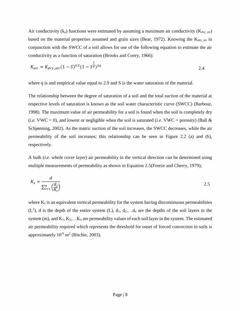
Air conductivity (ka) functions were estimated by assuming a maximum air conductivity (Kdry_air)
based on the material properties assumed and grain sizes (Bear, 1972). Knowing the Kdry_air in
conjunction with the SWCC of a soil allows for use of the following equation to estimate the air
conductivity as a function of saturation (Brooks and Corey, 1966):
𝐾𝑎𝑖𝑟 = 𝐾𝑑𝑟𝑦_𝑎𝑖𝑟(1 − 𝑆)0.5(1 − 𝑆1𝑞)2𝑞
2.4
where q is and empirical value equal to 2.9 and S is the water saturation of the material.
The relationship between the degree of saturation of a soil and the total suction of the material at
respective levels of saturation is known as the soil water characteristic curve (SWCC) (Barbour,
1998). The maximum value of air permeability for a soil is found when the soil is completely dry
(i.e. VWC = 0), and lowest or negligible when the soil is saturated (i.e. VWC = porosity) (Ball &
Schjønning, 2002). As the matric suction of the soil increases, the SWCC decreases, while the air
permeability of the soil increases; this relationship can be seen in Figure 2.2 (a) and (b),
respectively.
A bulk (i.e. whole cover layer) air permeability in the vertical direction can be determined using
multiple measurements of permeability as shown in Equation 2.5(Freeze and Cherry, 1979);
𝐾𝑧 =𝑑
∑ (𝑑𝑖
𝐾𝑖)𝑛
𝑖=1
2.5
where Kz is an equivalent vertical permeability for the system having discontinuous permeabilities
(L2), d is the depth of the entire system (L), d1, d2,…dn are the depths of the soil layers in the
system (m), and K1, K2,…Kn are permeability values of each soil layer in the system. The estimated
air permeability required which represents the threshold for onset of forced convection in soils is
approximately 10-9 m2 (Ritchie, 2003).

Page | 9
Figure 2.2 Relationship between soil water characteristic curve (a) and air permeability of a
soil (b). As the soil suction increases in the soil, a decline in the VWC is noted, while an increase
in the air coefficient of permeability is noted (D.G. Fredlund et al., 2012).
The upper and lower bound for air permeability is associated with the fully dry and saturated states
of the soil, respectively (D.G. Fredlund et al., 2012). As such, the air permeability can be described
in one of two ways: with respect to the saturation value of the soil (i.e., with respect to VWC), or
with respect to the suction of the soil (i.e. with respect to volumetric air content (VAC)).

Page | 10
2.2 Water Balance Method
The water balance method can be used to assess the processes controlling changes in the water
stored within a specified depth (volume) of soil. (Savenjie, 1997). The water balance method relies
on the in situ measurement of soil water contents along with climate data including precipitation
and atmospheric conditions from which potential evapotranspiration (PET) can be estimated. The
following components should be measured in order to actual evapotranspiration (AET) in a system:
• Total precipitation, including snowmelt (PPT);
• Actual evapotranspiration (AET);
• Runoff and Interflow (RI); and
• Net Percolation (NP).
By measuring or estimating the above parameters, 2.6 can be solved to determine an overall change
in storage (ΔS) within the system (modified from (Savenjie, 1997)):
∆𝑆 = 𝑃𝑃𝑇 − 𝐴𝐸 − 𝑅𝐼 − 𝑁𝑃 2.6
However, many of these parameters are difficult to measure accurately. In situations where there
is only one unknown in the system, the remainder of the equation can be solved by setting it
equivalent to 0 by assuming continuity and changing the unknown parameter until a null condition
is met.
2.2.1 Potential and Actual Evapotranspiration
ET is the amount of water that would be evaporated under an optimal set of conditions (e.g.,
unlimited supply of water) and can be computed from climatic inputs using Penman’s method
(Penman, 1948). Evapotranspiration is the combined effect of evaporation (the process by which
liquid water is transformed into the vapour phase via an energy input) and transpiration (the water
uptake by vegetation) (Chin, 2006). Evapotranspiration is defined as the quantity of water leaving
a soil per unit area, per unit time. A difficulty arises in differentiating between evaporation from
the ground and transpiration by plants when a vegetated surface is taken into consideration.

Page | 11
In practice, there are two primary terms used to describe the water loss from a system due to
evapotranspiration: PET and AET. These terms are typically used synonymously with potential
evaporation (PE) and actual evaporation (AE), respectively. Due to the difficulties in assessing
water movement through a soil, there have been hundreds of contrasting methods developed to
predict the AET and PET from a system over the years. The most generally accepted method of
prediction of PET is the Penman (1948) method, later adapted to the Penman-Monteith (1965)
method. This method utilizes a number data points measured using meteorological instrumentation
and is presented in Equation 2.7.
𝐸𝑇𝑜 =∆ ((𝑅𝑛 − 𝐺) + 𝜌𝑎𝑐𝑝(𝛿𝑒)𝑔𝑎)
∆ + 𝛾 (1 +𝑔𝑎
𝑔𝑠) 𝐿𝑣
2.7
where ETo is the water volume evaporated per unit time (mm s-1), Δ is the rate of change of
saturation specific humidity with air temperature (Pa K-1), Rn is the net irradiance (w m-2), G is the
ground heat flux (w m-2), ρa is the dry air density (kg m-3), cp is the specific heat capacity of air (J
kg-1 K-1), δe is the specific humidity (Pa), ga is the atmospheric conductance (m s-1), γ is the
psychrometric constant (~66 Pa K-1), gs is the surface conductance (m s-1), and Lv is the volumetric
latent heat of vaporization (MJ m-3).
The measurement of PET by the Penman-Monteith (1965) method assumes that the soil surface
remains saturated throughout the evaporation process. Unfortunately, this is typically never the
case in true real-world scenarios, and as such, the measured PET is typically an overestimate of
the actual evaporation (AET) occurring.
AET is the rate of water removal that the deposit actually experiences due to evaporation. The
AET/PET ratio is 1.0 when available water at the deposit surface is adequate. In typical soil and
mine waste deposits, the ratio falls below 1.0 and experiences temporal fluctuations due to a
number of factors, including rainfall, salinity changes, and surface desiccation. If the ratio is very
low (i.e., practically nil), then minimal water can be removed from the deposit by evaporation. The
following sub-sections describe the methods utilized to estimate the AET at the site.
Determining the actual evapotranspiration in field scenario is a difficult task due to the large
number of variables and influencing factors (density of vegetation, variable solar radiation,

Page | 12
variable wind velocities, etc.). Using the Penman-Monteith (1965) method to estimate the PET
allows for an estimate of the maximum evaporation rates from a specific vegetated area, however,
several methods can further refine this estimate to calculate an AET rate.
If the field capacity and wilting point of a soil are known, a linear relationship relating the AWHC
can be used to determine the AET from a soil as follows (Brooks et al., 2013).
𝐴𝐸𝑇 = 𝑃𝐸𝑇 ∗𝑉𝑊𝐶 − 𝑊𝑃
𝐹𝐶 − 𝑊𝑃 2.8
Using the above equation, when the soil moisture is at or near to the field capacity, the AET is
equivalent to the PET, whereas when the soil moisture is at or below the WP, the AET is equivalent
to 0. The remainder of the range between the FC and the WP will show a linear relationship
between the AET/PET ratios as determined from the equation. The measurement of field capacity
and wilting point are drawn directly from measurements of in situ Volumetric Water Content
(VWC), using methods described in Section 3.2.5.
2.2.2 Precipitation
Precipitation is formed as a rising mass of humid air cools to the dew point temperature. As the
rising mass of air cools, the evaporated moisture will condense around particulates in the air,
creating droplets of water (Fetter, 1994). When these water droplets reach a certain size, they will
begin descending to the earth, resulting in precipitation. In Fort McMurray, Alberta, this may occur
in the form of rainfall, hail, or snowfall.
Measurement of rainfall can be performed using an open topped container, and it has been shown
that the size of the opening has little effect on the total volume of rainfall measured (Fetter, 1994).
Rain gauges used at the CBIW are tipping bucket style rain gauge (TE525) with a CS705 snowfall
adapter containing ethylene glycol which melts snowfall and subsequently measures the snow
water equivalence (SWE) at the site.
In addition to measurement of SWE via the ethylene glycol measurement, prior to snowmelt
manual snow surveys are performed by SCL environmental field staff. In general, it can be said
that approximately 10% of the total snow depth is the equivalence of water in the snow pack.

Page | 13
However, as time progresses, and more snow falls, this number tends to become less accurate as
the snowpack is compressed under the weight of the overlying snow, resulting in a denser snow
pack. As such, manual snow surveys are required to obtain a more accurate density measurement
of the snow pack to correlate to an equivalent depth of water. The most accurate measurement of
snowpack occurs as close to spring melt as possible, as this is when the greatest amount of snow
is present at its most dense state.
A snow survey utilizes a thin walled tube driven into the snow pack. A field measurement of mass
of the tube and snow are taken, and the subsequent density of the snow can be calculated from the
known mass of the dry tube and dimensions of the tube. The snow water equivalence can be
calculated as follows in 2.9 (Pomeroy and Gray, 1995):
𝑆𝑊𝐸 =𝑑𝑠𝜌𝑠
𝜌𝑤 2.9
where ds is the average depth of the snow pack at the point of measurement, and ρs and ρw are the
average densities of the snow and water respectively.
2.2.3 Infiltration / Net Percolation
The process by which water enters the soil as a result of precipitation is known as infiltration (Chin,
2006). Infiltration is not to be confused with net percolation. Net percolation is a term which is
used to describe the movement of water through the soil within a specified soil body (i.e., a cover
system) and is the water which remains following all removal processes (evapotranspiration,
interflow, etc.), while infiltration is specific to the movement of water into the soil at the surface.
The capacity for infiltration for a specific soil is primarily determined by the amount of surface
cover material and the specific soil moisture properties. For a vegetated surface such as at the
CBIW, the infiltration capacity is typically higher than that of a bare soil as a result of flow
pathways through the soil surface resulting from vegetation stalks.
The net percolation will vary from the infiltration rate depending on the level of vegetation at the
surface, flow pathways within the subsurface, and various other influencing factors. Alternative
flow pathways may exist in the form of macro-pores and cracking at the surface which can greatly
increase net percolation rates through preferential bypass flow through which water can flow

Page | 14
significantly faster than flow through micropores, as governed by Darcian flow
(Saravanathiiban D.S. et al., 2014). Water flowing through continuous macropores essentially
results in water short-circuiting around the cover system and rooting zone of the plants. Water
entering the cracks may infiltrate into the vertical walls of the cracks but may also bypass the soil
entirely through the base of the crack; as a result, the majority of water balances do not
accommodate the potential for bypass flow.
2.2.4 Runoff & Interflow
In general, two forms of runoff are typically used to describe the potential overland runoff from a
given storm event: infiltration excess and saturation excess (Chin, 2006). Infiltration excess occurs
when the rainfall exceeds the infiltration capacity of the soil in question at the surface, whereas
saturation excess occurs when the soil is saturated at the surface, resulting in a decreased
infiltration rate. At first glance these may seem to indicate the same process, however, the
differentiation arises between what is used to describe and calculate the actual infiltration capacity
of the soils in each method. Infiltration excess limits its analysis to contributing roles of soil type
and land use, however, saturation excess runoff includes landscape position, local topography, and
soil depth.
The other component of runoff is interflow, which is the lateral flow of water in the subsurface.
Baseflow is the flow of water in the subsurface into the system and is typically independent of
rainfall events. Interflow is the subsurface flow of water which lands on the system and continues
to flow out of the system boundaries.

Page | 15
Chapter 3
Field and Laboratory Program
Instrumentation designed to measure the cover water balance had been previously installed by
OKC (2006) and was expanded upon by Fenske (2012). This chapter describes the field programs
undertaken at the SCL CBIW through the duration of this study (2012-2014), as well as the
instrumentation which was installed and monitored at the site and which was used as part of the
analyses undertaken in the present study.
The magnitude of convective airflow across the cover is controlled primarily by the air
permeability of the cover and underlying unsaturated coke and the air pressure deficiency present
within the waste below the cover. In order to assess the potential for convective airflow across the
cover system profile, a system of differential pressure sensors (pressure relative to atmospheric
pressure) was installed for this study at various depths across the covers and into the underlying
coke at multiple locations. This differential pressure monitoring system included a high accuracy
barometric pressure sensor to determine absolute pressure in the system. A component of this in
situ monitoring program included point measurements of air permeability in the cover profile for
all of the various material types.
3.1 Airflow Conceptual Model
The hypothesized cause of the convective airflow system being investigated at the CBIW is the
geometry of both the deposit and the berm adjacent to the deposit coupled with the porous nature
of the sand tailings and coke tailings and temperature gradients between subsurface and ambient
air. Both the sand tailings and coke are covered by a peat-clay mixture which provides a low-
permeability isolation boundary layer to the system. This cover system typically would inhibit air
and moisture movement into the stored materials, however, due to the unsaturated condition of the
coke, proximity of the coke to the edge of the berms downslope, and the temperature variances
across the cover system, a density dependant convective cell may develop.
This conceptual model is what is hypothesized to drive the convective airflow in the system,
however, due to the scale is difficult to measure and quantify. As such, in order to isolate the
conceptual model to the cover system, all analyses have been carried out across the cover system

Page | 16
with the assumption that any downward flowing air is driven towards the berm due to natural
topography of the deposit and airflow forcing caused by the temperature gradients down the slope.
This process may be investigated further with enhanced numerical modelling but is outside the
scope of this thesis.
When considering the design of the berm sloping at a downward angle and maintaining vadose
conditions throughout the slope, this temperature trend is likely maintained down the entire slope
of the berm, as the cover depth profile is approximately the same. In this situation, the more dense
air in the subsurface will tend to exit the tail of the slope. This action would then result in a
negative pressure in the subsurface which would then draw in air through the cover system at the
point of highest pressure gradient. It is this action which is likely driving any convective airflow
across the cover system.
3.2 Description of Test Covers and Existing Instrumentation
Fluid coke was hydraulically deposited and graded in 2004 to create two prototype watersheds,
each approximately 4.5 ha in area. Two-layer soil covers were then constructed overtop of the
deposited coke in the fall/winter of 2004. The cover was constructed with a negligible slope of less
than 1%. The lower layer consisted of a layer of salvaged glacial till overlain by a mixture of peat-
mineral soil (glacial till) salvaged by over-stripping surficial peat deposits prior to mining.
The purpose of these cover system trials was to assess the viability of various cover system designs
for reclamation of coke beaches. The two different cover systems were constructed as follows:
• Shallow cover system: a nominal depth of 40 cm, comprised of a 15 cm layer of peat-
mineral mix and an underlying layer of till with a depth of 25 cm
• Deep cover system: a nominal depth of 100 cm comprised of a 15 cm layer of peat-mineral
mix at the surface, and an underlying layer of till having a depth of 85 cm.
Installation of the field monitoring at the CBIW was undertaken by OKC (2006) with additional
site characterization and field testing undertaken by Fenske (2012). The field monitoring included
a climate station, soil profile monitoring as well as the construction of a collection lysimeter under
each cover. Details of each of these systems are outlined in the following subsections.

Page | 17
A complete summary of all existing OKC installed instrumentation is presented in Table 3.1. The
layout of the site is shown Figure 3.1 and Figure 3.2.
Table 3.1
Summary of existing instrumentation installed in each cover system and along adjacent berm
Location Instrumentation by OKC
(2004)
Deep Cover System
• Soil VWC sensors (8)
• Soil matric suction and
temperature sensors (8)
• Data acquisition system
Shallow Cover
System
• Soil VWC sensors (8)
• Soil matric suction and
temperature sensors (8)
• Meteorological station
• Data acquisition system

Page | 18
Figure 3.1 Aerial view of MLSB and specific location of project study area, including two
cover systems configuration

Page | 19
Figure 3.2 Aerial view of project study area showing two cover systems configuration
3.2.1 Meteorological Station
The meteorological station was installed in 2004 by OKC (O’Kane Consultants Inc., 2004) near
the centre of the shallow cover system. The monitoring consisted of a tipping bucket rain gauge
(Model TE525) as well as the following instrumentation mounted on a single tripod (Figure 3.3):
• Temperature and RH monitoring performed using a Betatherm 0.3K1A1A thermistor and
a Vaisala HUMICAP® 180 capacitive RH sensor, respectively; both of which are built into
the single instrument that is the Campbell Scientific Model HMP45CF probe.
• Wind speed and 360o direction measurement done using an R.M. Young Model 05103
anemometer.
• Net radiation measured using an NR-Lite Net Radiometer mounted 2.5 m above the surface
of the cover system.

Page | 20
Figure 3.3 Meteorological station installed on shallow cover at MLSB CBIW (September 24,
2003)
3.2.2 Automated Soil Monitoring Stations
OKC installed automated soil monitoring stations and associated data acquisition systems on each
cover system in 2004. The soil monitoring stations included sensors to monitor soil temperature
and matric suction (Campbell Scientific 229 sensors), and volumetric water content (Campbell
Scientific 616 TDR sensors). The installation depths and sensors installed at each depth on the
deep cover system are outlined in Table 3.2, and for the shallow cover system in
Installation Depth (cm from surface)
5
10
20
25
30
40
90
180
Table 3.3. Each sensor type (CS229 and CS616) was installed alongside each other at equivalent
depths.

Page | 21
Table 3.2
Soil monitoring instrumentation depths installed by OKC at Shallow Cover System in 2004
Installation Depth (cm from surface)
5
10
20
25
30
40
90
180
Table 3.3
Soil monitoring instrumentation depths installed by OKC at Deep Cover System in 2004
Installation Depth (cm from surface)
5
20
30
45
70
90
100
180
The soil monitoring sensors were wired into a CR1000 datalogger, manufactured by Campbell
Scientific. Each cover system uses its own datalogger for data collection and storage purposes.
The soil monitoring systems and datalogging equipment were located at S02 and D02 in Figure
3.4.
3.2.3 Infiltration, Net Percolation, and Runoff/Interflow
At the CBIW, the net percolation through the cover system was measured in situ using a lysimeter
until the close of 2006. Following 2006, no net percolation measurements were recorded. The
lysimeters were designed and installed by OKC in 2004, and have a diameter of 2.44 m and a
height of 2.5 m (O’Kane Consultants Inc., 2004). The tanks were hollow, and as such, required
that the inside be filled with native material to the same level of compaction of the material outside
the tank to ensure a representative measurement of percolation. Each tank was installed to a depth
of 2.5 m below the surface of the coke, measured from the bottom of the lysimeter tank, resulting
in the top of the lysimeter resting at the base of each respective cover system. This allowed for
direct measurement of total net percolation through the cover systems. Measurements of water

Page | 22
volume in the lysimeter were facilitated using a piezometer installed in the centre of each lysimeter,
with regular measurements of water height recorded. The piezometer tube also allowed for the
removal of water as required.
At the close of the 2006 monitoring year, no percolation was recorded through the shallow cover
system during the 2 year monitoring period, while only 21.6 mm of percolation were recorded
through the deep cover system for the same period (Fenske, 2012).
In the system being studied at the CBIW, changes in surface grade are negligible, and as such, no
runoff or interflow has been measured or recorded since the commencement of the project. For the
purposes of analysis, the runoff and interflow in the system is assumed to be negligible.
3.2.4 Soil Temperature and Matric Suction
The measurement of the soil temperature and the soil matric suction is carried out using a Campbell
Scientific 229 (CS229) matric potential sensor. The CS229 sensor uses a heating element and a
thermocouple which is encapsulated in epoxy within a hypodermic needle. This setup is then
encased in a porous ceramic matrix which allows for equilibration with the surrounding soil
moisture. The air entry value (i.e. minimum suction measurement threshold of the sensor) is 10
kPa, and the maximum measurement potential of the sensor is 2500 kPa of suction.
The soil suction in the soil surrounding the CS229 sensor is measured by using a current exciting
module to induce an electrical current through the thermocouple. This electrical current causes an
increase in the temperature of the thermocouple, and the magnitude of the temperature rise is
dependent on the amount of water content of the ceramic matrix surrounding the thermocouple
setup. The ceramic is assumed to be in equilibrium with the suction within the surrounding soil.
The rate of temperature rise is then related to the matric suction of the soil using a second order
polynomial derived from a laboratory calibration of each sensor. This calibration was carried out
by OKC prior to installation. The temperature of the soil surrounding the CS229 sensor must be
taken and recorded prior to each reading of the sensor using the built in thermocouple in order to
provide a reference temperature for the total temperature rise. As a consequence, this sensor
functions as both a matric suction sensor and a soil temperature sensor.

Page | 23
The volume of water in the air within unsaturated soils can be assumed to be saturated when above
wilting point. The saturation vapour pressure of the air within soil voids can be calculated using
Equation 3.1 (National Oceanic Atmospheric Institute, 2015).
𝑃𝑠𝑎𝑡 = 6.11 𝑥 10(7.5 𝑥 𝑇
237.3+𝑇) 3.1
The vapour pressure of the soil air can be determined using Equation 3.2 (National Oceanic
Atmospheric Institute, 2015).
𝑅𝐻 =𝑃𝑣𝑎𝑝
𝑃𝑠𝑎𝑡 3.2
The calculated maximum potential moisture removal rates are based on the calculated airflow and
the moisture removal potential (discussed in Sections 5.5.1 and 5.3.1, respectively). These values
are calculated based on the measured temperature conditions within the cover system and the air.
The estimated moisture removal rate is calculated as follows:
𝑇𝑣 = 𝑓𝑔 ∗ 𝑀𝑎 3.3
where Tv is the total volume of moisture removed (grams), fg is the total airflow rate per day
(m3/day), and Ma is the total moisture availability for removal from the soil profile (grams/m3).
The total moisture availability for removal is assumed to be the difference between the actual
vapour pressure of the ambient air, and the saturated vapour pressure of the soil void air.
3.2.5 Volumetric Water Content
The soil volumetric water content (VWC) is measured using Campbell Scientific 616 (CS616)
time-domain reflectometry (TDR) sensors. These sensors are based on water content reflectometry
technology and are capable of measuring a wide range of water content in various soil materials.
The CS616 probe consists of two 300 mm long stainless steel probes connected to a circuit board
for the measurement system. The circuit board is encapsulated in epoxy to protect the wiring from
soil moisture. A measurement of dielectric permittivity is taken by allowing an electromagnetic
pulse to propagate along a waveguide surrounded by soil, using the stainless-steel rods as a
guideline for the wave (Hu et al., 2006). The travel time of the electromagnetic wave through the
Page | 24
soil, and the reflection of the pulse back to the sensor is measured, and is correlated back to the
soil VWC using the Topp et al., (1980) equation. This equation (1980) is generally considered to
be universal and can be applied directly to measured dielectric permittivity to determine soil VWC.
There are exceptions to the “universal” nature of the Topp et al. (1980) equation, which includes
unsaturated clay soils, however, these exceptions do not affect this study and as such the Topp et
al. (1980) equation can be used directly.
3.3 Instrumentation Installed as a Component of this Thesis
In order to adapt the current monitoring system to be able to measure differential airflow, the
author designed and installed a differential pressure monitoring system across the cover system.
The installation locations are shown in Figure 3.4. The details of these systems are outlined in
Table 3.4.
Figure 3.4 Detailed instrumentation installation locations at the coke beach instrumented
watershed

Page | 25
Table 3.4
Differential Pressure Monitoring Systems installed by the Author in 2012
Location Instrumentation as part of this
study (Spring 2013)
Deep Cover System
• Differential gas pressure
sensors, 3 locations (D01, D02,
D03), 3 sensors each location
• Data acquisition systems
Shallow Cover
System
• Differential gas pressure
sensors, 3 locations (S01, S02,
S03), 3 sensors each location
• Data acquisition systems
Figure 3.5 Installing gas probes at monitoring location using AMS International system.
Gas inlet ports were installed using the AMS International® gas sampler (Figure 3.5). The
advantage of this system is that it uses dedicated vapour sampling tips which can be installed in
the subsurface without pre-boring. This system utilizes steel gas vapour tips attached to
fluoropolymer tubing which is then fed through a hollow steel pipe. Using a manual impact
hammer, this steel pipe is gradually hammered into the ground to the desired depth. As the steel
Page | 26
pipe forces the gas vapour tip further into the ground, extensions to the steel pipe are added to
accommodate the additional depth to which the gas vapour tip is being placed.
The differential pressure measurements were obtained using differential pressure monitoring
sensors. Table 3.5 shows the installation depths and identifications assigned to each sensor
installation on top of the CBIW, as well as the GPS coordinate of each instrumentation cluster.
Table 3.5
Installation depths and identification numbers for differential pressure sensors at each cover
system
Site ID
Full
Installation
ID
Depth
Below
Surface
(m)
Easting Northing
Dee
p C
over
D01
D01-30 0.33
459975.36 6323805.46 D01-110 1.1
D01-200 2
D02
D02-30 0.5
460063.8 6323804.83 D02-110 1.1
D02-200 2
D03
D03-30 0.5
460113.59 6323810.02 D03-110 1.1
D03-200 2
Shal
low
Cover
S01
S01-30 0.25
459985.51 6323706.39 S01-70 1.1
S01-200 2
S02
S02-30 0.25
460047.83 6323702.23 S02-80 1.1
S02-190 1.9
S03
S03-50 0.25
460099.64 6323709.41 S03-110 1.1
S03-200 1.5
The measurement of differential pressure was performed using PA-699 differential air pressure
sensor and is manufactured by Sontay Instruments and distributed by Omni Instruments. The PA-
699 differential pressure sensor can measure low-range differential gas pressure (0-100 Pa). The
sensors are powered by an external 1.2 Ah sealed lead-acid (SLA) battery. The differential pressure
sensors were connected to Logbox-AA datalogging systems, manufactured by Novus®. These

Page | 27
systems are capable of recording data from two analog sensors per unit. As such, for locations with
more than two differential pressure sensors, two datalogging units were required. The completed
monitoring system can be seen in Figure 3.6.
Figure 3.6 Completed differential pressure monitoring system and data acquisition system
Each differential pressure sensor utilizes a low pressure and a high-pressure port, with the
difference in pressure across the two ports resulting in a voltage drop which can be converted to a
relative differential pressure. The differential pressure measurements are made at the same
elevation and consequently no pressure corrections for hydrostatic air pressures or density were
applied to the measurements.

Page | 28
Figure 3.7 Differential pressure sensor configuration.
Early iterations of the project design included the measurement of differential pressures along the
western berm of MLSB, adjacent to the CBIW. Differential pressure monitoring systems were
installed as indicated in Table 3.6.

Page | 29
Table 3.6
Installation depths and identification numbers for differential pressure sensors on side berm of
MLSB
Site ID
Full
Installation
ID
Depth
Below
Surface
(m)
Easting Northing M
LS
B B
erm
B01
B01-40 0.4
459715.15 6323764.01 B01-100 1
B01-200 2
B02
B02-40 0.4
459661.8 6323766.98 B02-100 1
B02-200 2
B03
B03-40 0.4
459767.13 6323763.06 B03-100 1
B03-200 2
B04
B04-40 0.4
459822.87 6323756.06 B04-100 1
B04-200 2
B05
B05-40 0.4
459874.2 6323751.55 B04-100 1
B04-200 2
The sensors listen in Table 3.6 were monitored early in the investigative process, however,
monitoring was eventually ceased due to lack of results/correlation and were omitted from this
thesis.
3.3.1 Barometric Pressure
The measurement of the ambient barometric pressure was done using a Vaisala BAROCAP®
Digital Barometer PTB210. This sensor was selected due to its high accuracy (+/- 15 Pa using a
digital output), and its suitability for harsh environments, such as the exposed condition on top of
MLSB. Due to the lack of appropriate dataloggers at the actual site of the study (MLSB CBIW),
the PTB210 barometer was installed approximately 300 m away at the same elevation at an
alternate OKC datalogging system. The sensor was shielded using a shield designed and
distributed by the manufacturer of the sensor. The purpose of the shielding was to prevent
influences from solar radiation and wind effects. This datalogger was a CR1000 manufactured by

Page | 30
Campbell Scientific. This data was downloaded by OKC on quarterly basis and forwarded to the
author.
3.4 Field Testing Program
The field testing program consisted of air permeability testing carried out by the author, assisted
by University of Saskatchewan Research Engineer, Dyan Pratt.
3.4.1 Air Permeability Testing
Air permeability testing was carried out using a method developed by Rodgers (2008), and further
utilized in Huang et al. (2014) and Huang et al. (2016) at the University of Saskatchewan. This air
permeameter, shown in Figure 3.8, was tested at the CBIW by Rodgers (2008) as a component of
her master’s research. These measurements were used to supplement the results obtained in this
study.

Page | 31
Figure 3.8 Conceptual design or air permeameter used in determination of air permeability
(not to scale).
The system outlined in Figure 3.8 was adapted such that it could be driven to a specified depth
into the soil cover profile using the AMS International soil gas probe kit used to install the DP
sensors. The soil vapour probe is approximately 3 cm in diameter, and approximately 15 cm long.
Two hoses were connected to the retractable gas vapour sampler. The airflow entered the vapour
sampler through one hose, where it was allowed to diffuse into the surrounding soil until a constant
pressure condition was achieved, as measured from the second hose attached to a pressure sensor
at the surface. The functionality of the system was determined using the permanent vapour
sampling tips installed to measure differential pressures; these were located between 2-3 m from
the permeameter location. The airflow rate and air pressures through the system were recorded
using an automated flow meter. The airflow rates and pressures measured across the screened
length were interpreted using a numerical flow model (SEEP/W, Geo-Slope International 2012) to
estimate permeability (K). The flow rates (Q) and pressure responses (dH) were used to set up a

Page | 32
2-D numerical model using axisymmetric coordinate system to simulate a pumping well using
Geostudio SEEP/W software. The numerical model utilized a unit geometry (1 m2 cross sectional
area); the boundary conditions of the unit geometry were assumed to be a no-flow boundary, while
the surface of the soil geometry was assumed to have a pressure of 0 kPa (no differential pressure
gradient between subsurface air and ambient). The point of the drive-point permeameter was
assumed to be a constant head as the test was run until a constant pressure head was measured by
the permeater test gauges. The numerical model was run in steady state using an arbitrary geometry
but with a nominal differential head and conductivity of unity to define a shape factor (F) for the
test (i.e. F = Q/(Kdh). This shape factor was then used to obtain a value of K from the field tests
for the test specific flowrates and measured pressure responses.
Air permeability was measured for the till cover layer and the underlying coke in September, 2013.
The testing locations were isolated to S01 and D01 due to limitations associated with moving
equipment across the rugged terrain of the cover system. Each cover system and underlying coke
were tested at each trial cover system location, as per Table 3.7
Table 3.7
Air Permeability Test Depths and Flow Rates
Shallow Cover System Deep Cover System
80 cm 20 cm 110 cm 80 cm 20 cm
Air Permeameter
Flow Rate
5 5 5 5 5
10 10 10 10 10
15 15 15 15 15
20 20 20 20 20
It should be noted that these air permeability testing represent conditions at a single point in time,
and as such, for a single soil VWC. The procedure to simulate air permeability (K-air) was to
simply simulate the test geometry (e.g. screen depth and length) using differential air heads (dh)
of unity and a unit media fluid conductivity (i.e. K-air = 1). The simulation then defines the
relationship between differential head between the screen and the atmosphere and flow rate (Q).
This defines the shape factor (F) which is set equal to Q/(Kdh). The value of K can then be
calculated from the actual measured values of Q and dh from the field test.

Page | 33
Chapter 4
Presentation of Data
This chapter presents and discusses particular observations pertinent to the hypothesis of enhanced
drying of the covers due to convective airflow. Soil volumetric water content (VWC) and suction
data collected from CS616 and CS29 sensors, respectively, are presented in Appendix A. The full
set of data from all sensors used while investigating this thesis is included as an electronic
supplement (Appendix B); this data is used in Chapter 5 (Analyses) to evaluate the water balance
for the covers. The specific elements of this data set that are important to the potential for
convective airflow include the following:
• The magnitude, direction, and timing of differential pressures between the atmosphere and
underlying coke which may be creating conditions for airflow.
• Soil cover, coke, and air temperatures to identify the timing and magnitude of the
temperature contrasts which may create differences in air density which may in turn lead
airflow and subsequent differential pressures.
Taken together, these observations provide evidence as to the timing and extent of potential
mechanisms for convective airflow or evidence of enhanced drying. The extent of this drying will
be further quantified in Section 5 (Analyses) by estimating the contribution of the enhanced drying
in the cover water balance.
This section of the thesis will also present the data obtained from the monitoring of pressure
differentials and the measurement of in situ air permeability.
4.1 Temperature Gradient across Cover Systems
The potential for free convection to develop across the cover can also be illustrated by looking at
the temperature gradient between the atmosphere and the underlying unsaturated coke. The
detailed temperature data presented in Appendix A show the deep soil temperatures to fluctuate
seasonally between 5oC and 15oC. The deep soil air temperature can be used to represent the
temperature of the bulk air mass in the subsurface and is subsequently used to assess temperature
gradients relative to the ambient atmosphere.

Page | 34
The temperature difference between the ambient and the deep soil air temperatures at the shallow
cover system is shown in Figure 4.1 for the 2013 monitoring year, while Figure 4.2 shows the
same for the deep cover system; these figures were isolated to months in which the soil was
unfrozen in order to highlight temperature gradients which would allow for unimpeded airflow
through unfrozen soil. Months not shown were during periods in which the cover system was
frozen, preventing effective airflow. It can be seen that starting in early May and continuing
throughout the duration of the summer the temperature in the subsurface is much lower than the
ambient atmospheric temperature. As a consequence, the subsurface air is more dense than ambient
air and consequently in the presence of a sloping geometry could result in downward airflow
through the cover and underlying coke out towards the dyke slope and the outlet drains installed
within the sand dyke.
Figure 4.1 2013 differential air temperature, shallow cover system
-10
-5
0
5
10
15
20
25
30
Te
mp
era
ture
(°C
)
Air Temperature
Soil Temperature (2.0 m)

Page | 35
Figure 4.2 2013 differential air temperature, deep cover system
Temperature trends in 2014 showed similar results, indicating more dense air in the subsurface,
which could result in downward flow for the duration of the summer months (Figure 4.3, Figure
4.4); again, these figures were isolated to months in which the soil was unfrozen in order to
highlight temperature gradients which would allow for unimpeded airflow through unfrozen soil.
Months not shown were during periods in which the cover system was frozen, preventing effective
airflow.
-10
-5
0
5
10
15
20
25
30
Tem
pera
ture
(°C
)Air Temperature
Soil Temperature (2.0 m)
Page | 36
Figure 4.3 2014 differential air temperature, shallow cover system
Figure 4.4 2014 differential air temperature, deep cover system
The large temperature gradient present predominantly during spring/summer at both locations
proves conceptually that the necessary conditions for convective airflow exist. The determination
of true convective airflow requires further analysis and will be presented later in the thesis.
-10
-5
0
5
10
15
20
25
30
Te
mp
era
ture
(°C
)Air Temperature
Soil Temperature (2.0 m)
-10
-5
0
5
10
15
20
25
30
Te
mp
era
ture
(°C
)
Air Temperature
Soil Temperature (2.0 m)

Page | 37
4.2 In situ Differential Pressure Monitoring
The sensors available for monitoring the differential pressure in the cover system were only
capable of monitoring differential pressure between an inlet (low pressure) and outlet (high
pressure) port. The effect of an elevation gradient (i.e. gravity gradient) on flow is also essentially
taken into account by the fact that the difference in the two pressures (soil and atmosphere) are
measured at a common elevation. As a result, the focus of this discussion will be on the measured
difference between the high pressure outlet and the low pressure outlet and is referred to as the
measured differential pressure (dP). The dP sensor is only capable of measuring a positive value
for dP. A negative dP (i.e. the inlet pressure becomes higher than the outlet pressure) cannot be
measured.
In 2013 the sensor configuration was connected such that the inlet port was connected to the
subsurface measurement points and the outlet port was vented to the atmosphere. Detection of a
differential pressure was then associated with lower pressures within the soil profile than in the
air. This configuration was reversed in 2014 to evaluate if dP creating upward airflow in the
system. As such, the sensor configuration was set up differently for each monitoring year. In 2013,
the only measurable differential air pressure measurements occurred when atmospheric pressure
was greater than soil air pressure, while in 2014 the only measurable differential pressures where
for the period when soil air pressures were greater than atmospheric pressures. The subsequent
sections detail the differential pressure data measured at each location during each monitoring
setup.
The fluctuations in dP over the course of 2013 at all 3 shallow cover system monitoring locations
(S01, S02, S03) are presented in the following 3 figures (Figure 4.5, Figure 4.6, Figure 4.7). The
fluctuations in dP over the course of 2013 at all 3 deep cover system monitoring locations (D01,
D02, D03) are presented in the following 3 figures (Figure 4.8, Figure 4.9, Figure 4.10).

Page | 38
Figure 4.5 Differential pressure measured at S01 (2013).
-70
-60
-50
-40
-30
-20
-10
0
10D
iffe
ren
tia
l Pre
ss
ure
(P
a)
0.3 m
-70
-60
-50
-40
-30
-20
-10
0
10
Dif
fere
nti
al P
res
su
re (P
a)
0.7 m
-70
-60
-50
-40
-30
-20
-10
0
10
Dif
fere
nti
al P
res
su
re (P
a)
1.7 m

Page | 39
Figure 4.6 Differential pressure measured at S02 (2013).
-70
-60
-50
-40
-30
-20
-10
0
10D
iffe
ren
tia
l Pre
ss
ure
(P
a)
0.3 m
-70
-60
-50
-40
-30
-20
-10
0
10
Dif
fere
nti
al P
res
su
re (P
a)
0.7 m
-70
-60
-50
-40
-30
-20
-10
0
10
Dif
fere
nti
al P
res
su
re (P
a)
1.7 m

Page | 40
Figure 4.7 Differential pressure measured at S03 (2013).
-70
-60
-50
-40
-30
-20
-10
0
10D
iffe
ren
tia
l Pre
ss
ure
(P
a)
0.3 m
-70
-60
-50
-40
-30
-20
-10
0
10
Dif
fere
nti
al P
res
su
re (P
a)
0.7 m
-10
0
10
20
30
40
50
60
70
Dif
fere
nti
al P
res
su
re (P
a)
1.7 m
Sensor/Logger failure resulted in zero readings at S03

Page | 41
Figure 4.8 Differential pressure measured at D01 (2013).
-70
-60
-50
-40
-30
-20
-10
0
10D
iffe
ren
tia
l Pre
ss
ure
(P
a)
0.3 m
-70
-60
-50
-40
-30
-20
-10
0
10
Dif
fere
nti
al P
res
su
re (P
a)
0.7 m
-70
-60
-50
-40
-30
-20
-10
0
10
Dif
fere
nti
al P
res
su
re (P
a)
1.7 m

Page | 42
Figure 4.9 Differential pressure measured at D02 (2013).
-70
-60
-50
-40
-30
-20
-10
0
10D
iffe
ren
tia
l Pre
ss
ure
(P
a)
0.3 m
-70
-60
-50
-40
-30
-20
-10
0
10
Dif
fere
nti
al P
res
su
re (P
a)
0.7 m
-70
-60
-50
-40
-30
-20
-10
0
10
Dif
fere
nti
al P
res
su
re (P
a)
1.7 m

Page | 43
Figure 4.10 Differential pressure measured at D03 (2013).
-70
-60
-50
-40
-30
-20
-10
0
10D
iffe
ren
tia
l Pre
ss
ure
(P
a)
0.3 m
-70
-60
-50
-40
-30
-20
-10
0
10
Dif
fere
nti
al P
res
su
re (P
a)
0.7 m
-70
-60
-50
-40
-30
-20
-10
0
10
Dif
fere
nti
al P
res
su
re (P
a)
1.7 m

Page | 44
From the presented results it can be seen that measured differential pressures at both cover systems
vary throughout the season in 2013; however, the highest values generally occur in early spring
and then gradually decrease over the summer. Generally speaking, the highest differential
pressures occurred on days when the ambient temperature was substantially higher than the
subsurface temperature, and highest differential pressures were noted in late morning and early
afternoon. Most nighttime differential pressures were low or zero due to a thermal, or near thermal
equilibrium condition between the ambient temperature and subsurface temperature. The higher
differential pressures measured in spring do not necessarily mean that airflow was highest during
that time since consideration also needs to be given to the air permeability at any given point in
time. It should be noted that the deep sensors at S03 failed due to an unknown issue with the
datalogger, resulting in no results shown in Figure 4.7.
The daily variations in differential pressure are difficult to extrapolate from Figures Figure 4.5
through Figure 4.10 due to the large volume of data. In order to illustrate the daily cycle in
differential pressure, three dates were selected to represent spring to late summer conditions in
2013. The daily changes at both the shallow and the deep cover system are presented for May 16
to 18 (Figure 4.11 and Figure 4.12, respectively), June 16 to June 18 (Figure 4.13 and Figure 4.14,
respectively), and August 16 to 18 (Figure 4.15 and Figure 4.16, respectively). These days show
how the daily differential pressure gradients fluctuated throughout the monitoring season with
respect to temperature gradients across the cover systems.

Page | 45
Figure 4.11 Daily variations in measured differential pressure at S02, May 16 to 18, 2013
Figure 4.12 Daily variations in measured differential pressure at D02, May 16 to 18, 2013
0
5
10
15
20
25
30
-10
-9
-8
-7
-6
-5
-4
-3
-2
-1
0
Te
mp
era
ture
(°C
)
Dif
fere
nti
al P
res
su
re (P
a)
Differential Pressure - S02 Soil Temperature (2 m) Air Temperature
0
5
10
15
20
25
30
-10
-9
-8
-7
-6
-5
-4
-3
-2
-1
0
Te
mp
era
ture
(°C
)
Dif
fere
nti
al P
res
su
re (P
a)
Differential Pressure Soil Temperature (2 m) Air Temperature

Page | 46
Figure 4.13 Daily variations in measured differential pressure at S02, June 16 to 18, 2013
Figure 4.14 Daily variations in measured differential pressure at D02, June 16 to 18, 2013
0
5
10
15
20
25
-10
-9
-8
-7
-6
-5
-4
-3
-2
-1
0
Te
mp
era
ture
(°C
)
Dif
fere
nti
al P
res
su
re (P
a)
Differential Pressure - S02 Soil Temperature (2 m) Air Temperature
0
5
10
15
20
25
-10
-9
-8
-7
-6
-5
-4
-3
-2
-1
0
Te
mp
era
ture
(°C
)
Dif
fere
nti
al P
res
su
re (P
a)
Differential Pressure Soil Temperature (2 m) Air Temperature

Page | 47
Figure 4.15 Daily variations in measured differential pressure at S02, August 16 to 18, 2013
Figure 4.16 Daily variations in measured differential pressure at D02, August 16 to 18, 2013
0
5
10
15
20
25
30
-10
-9
-8
-7
-6
-5
-4
-3
-2
-1
0
Te
mp
era
ture
(°C
)
Dif
fere
nti
al P
res
su
re (P
a)
Differential Pressure - S02 Soil Temperature (2 m) Air Temperature
0
5
10
15
20
25
30
-10
-9
-8
-7
-6
-5
-4
-3
-2
-1
0
Te
mp
era
ture
(°C
)
Dif
fere
nti
al P
res
su
re (P
a)
Differential Pressure Soil Temperature (2 m) Air Temperature

Page | 48
It can be seen by Figure 4.12 through Figure 4.16 that the differential pressure consistently showed
a downward pressure gradient consistently through the monitoring season in 2013. This gradient
saw its highest value in June, 2013, and lowest at the end of the summer (August). Also shown in
Figure 4.12 through Figure 4.16 is the difference in temperatures between the soil and the ambient
atmosphere; these temperature gradients show a peak value in June alongside the same times that
peak differential pressures are measured, while in August, the temperature gradient declines due
to an increase in soil temperature, which is reflected in the lower values of differential pressure
occurring during the day.
The predominant differential pressure measured at each cover system was between 0 and -10 Pa
relative to atmospheric. Each monitoring location showed a different average differential pressure,
when considering only non-zero measured differential pressures. The occurrence frequency,
average, and standard deviation of non-zero differential pressures is presented in Figure 4.17 for
the shallow cover system, and Figure 4.18 at the deep cover system.
Figure 4.17 Histogram of measured non-zero DP values at Shallow Cover System
Table 4.1
Statistical Data of Measured Differential Pressures at Shallow Cover System Monitoring Location
Average of Non-Zero DP Values
Standard Deviation of Non-Zero DP Values
Percentage of Values Non-Zero DP
S01 -3.2 4.3 23
S02 -5.6 12.9 33%
S03 -7.3 15.7 10%

Page | 49
Figure 4.18 Histogram of measured non-zero DP values at deep cover system
Table 4.2
Statistical Data of Measured Differential Pressures at Deep Cover System Monitoring Location
Average of Non-Zero DP Values
Standard Deviation of Non-Zero DP Values
Percentage of Values Non-Zero DP
D01 -2.4 2.4 44%
D02 -12.2 20.7 15%
D03 -3.1 14.1 22%
Both S01 and D01 showed a similar average measured DP when compared to each other, indicating
that the pressure gradient across each cover system is comparable at these locations. However,
D02 appeared anomalous as it showed an average differential pressure nearly double that of any
other average differential pressure, while at D03 showed an average differential pressure nearly
half that of its shallow cover system counterpart. These variations may be a result of localized
surface cracking, variations in local soil moisture content, or variations in subsurface airflow
patterns affecting pressure measurements across the cover system or variations in water content
affecting local gas transmission rates through the soil cover systems.
The maximum pressure differentials at the shallow and deep cover systems (e.g. 60-70 pa) are
greater than those reported in the waste rock case studies described by Phillips (2009) where large
airflows were characterized utilizing a similar monitoring system. For example, Phillips (2009)
observed that only small differential air pressures (<10 Pa) created by temperature differences
were able to generate airflow across the surface of a waste rock dump in excess of 1 m/s. Although
0
500
1000
1500
2000
2500
3000
3500
4000
4500
-60-50-40-30-20-15-10-5-0.1
Nu
mb
er
of
Occu
rre
nce
s
Measured Differential Pressure Range (Pa)

Page | 50
the air permeability of a waste rock dump is likely to be much higher that the CBIW covers, the
higher differential pressures measured as part of this study indicate there is a potential for
convective airflow to occur, particularly through any high-permeability cracks which may appear
at the surface of the cover system.
4.2.1 2014 Monitoring Year
In 2014 the differential pressure measurements represent the potential for upward flow. These
results are shown in Figure 4.19 through Figure 4.24.
It can be seen that the differential air pressures (soil air pressure minus atmospheric pressure) are
much lower than the results for 2013 (atmospheric minus soil air pressure). The highest potential
for upward airflow is seen between June and July of 2014. Prior to May 2014, the differential
pressure measurements showed predominantly downward pressure differentials at both D01 and
S01, which indicate a high potential for downward flow; however, due to the freezing of the cover
system, it is unlikely any significant airflow actually occurred during this time.
The measured DP at each cover system was reduced to shorter time intervals in order to show daily
variations in DP alongside temperature differences across the cover system relative to ambient
atmospheric temperature. The daily changes at both the shallow and the deep cover system in 2014
are presented for May 16 to 18 (Figure 4.11 and Figure 4.12, respectively), June 16 to18 (Figure
4.13 and Figure 4.14, respectively), and July 16 to 18 (
Figure 4.15 and Figure 4.16, respectively). No measurements are shown for August, 2014 as
monitoring was ceased at the close of July, 2014.
Page | 51
Figure 4.19 2014 Differential pressure for S01; sensor direction reversed May 15, 2014
-10
0
10
20
30
40
50
60
70D
iffe
ren
tia
l Pre
ss
ure
(P
a)
0.3 m
-10
0
10
20
30
40
50
60
70
Dif
fere
nti
al P
res
su
re (P
a)
0.7 m
-10
0
10
20
30
40
50
60
70
Dif
fere
nti
al P
res
su
re (P
a)
1.7 m

Page | 52
Figure 4.20 2014 Differential pressure for S02; sensor direction reversed May 15, 2014
-10
0
10
20
30
40
50
60
70D
iffe
ren
tia
l Pre
ss
ure
(P
a)
0.3 m
-10
0
10
20
30
40
50
60
70
Dif
fere
nti
al P
res
su
re (P
a)
0.7 m
-10
0
10
20
30
40
50
60
70
Dif
fere
nti
al P
res
su
re (P
a)
1.7 m

Page | 53
Figure 4.21 2014 Differential pressure for S03; sensor direction reversed May 15, 2014
-10
0
10
20
30
40
50
60
70D
iffe
ren
tia
l Pre
ss
ure
(P
a)
0.3 m
-10
0
10
20
30
40
50
60
70
Dif
fere
nti
al P
res
su
re (P
a)
0.7 m
-10
0
10
20
30
40
50
60
70
Dif
fere
nti
al P
res
su
re (P
a)
1.7 m

Page | 54
Figure 4.22 2014 Differential pressure for D01; sensor direction reversed May 15, 2014
-10
0
10
20
30
40
50
60
70D
iffe
ren
tia
l Pre
ss
ure
(P
a)
0.3 m
-10
0
10
20
30
40
50
60
70
Dif
fere
nti
al P
res
su
re (P
a)
0.7 m
-10
0
10
20
30
40
50
60
70
Dif
fere
nti
al P
res
su
re (P
a)
1.7 m

Page | 55
Figure 4.23 2014 Differential pressure for D02; sensor direction reversed May 15, 2014
-10
0
10
20
30
40
50
60
70D
iffe
ren
tia
l Pre
ss
ure
(P
a)
0.3 m
-10
0
10
20
30
40
50
60
70
Dif
fere
nti
al P
res
su
re (P
a)
0.7 m
-10
0
10
20
30
40
50
60
70
Dif
fere
nti
al P
res
su
re (P
a)
1.7 m

Page | 56
Figure 4.24 2014 Differential pressure for D02; sensor direction reversed May 15, 2014
-10
0
10
20
30
40
50
60
70D
iffe
ren
tia
l Pre
ss
ure
(P
a)
0.3 m
-10
0
10
20
30
40
50
60
70
Dif
fere
nti
al P
res
su
re (P
a)
0.7 m
-10
0
10
20
30
40
50
60
70
Dif
fere
nti
al P
res
su
re (P
a)
1.7 m

Page | 57
Figure 4.25 Daily variations in measured differential pressure at S02, May 16 to 18, 2014
Figure 4.26 Daily variations in measured differential pressure at S02, June 16 to 18, 2014
0
2
4
6
8
10
12
14
16
18
20
-10
-8
-6
-4
-2
0
2
Te
mp
era
ture
(°C
)
Dif
fere
nti
al P
res
su
re (P
a)
Differential Pressure - S02 Soil Temperature (2 m) Air Temperature
0
5
10
15
20
25
-10
-8
-6
-4
-2
0
2
Te
mp
era
ture
(°C
)
Dif
fere
nti
al P
res
su
re (P
a)
Differential Pressure - S02 Soil Temperature (2 m) Air Temperature

Page | 58
Figure 4.27 Daily variations in measured differential pressure at S02, July 16 to 18, 2014
Figure 4.28 Daily variations in measured differential pressure at D02, May 16 to 18, 2014
0
5
10
15
20
25
30
-10
-9
-8
-7
-6
-5
-4
-3
-2
-1
0
Te
mp
era
ture
(°C
)
Dif
fere
nti
al P
res
su
re (P
a)
Differential Pressure - S02 Soil Temperature (2 m) Air Temperature
0
2
4
6
8
10
12
14
16
18
20
-10
-8
-6
-4
-2
0
2
Te
mp
era
ture
(°C
)
Dif
fere
nti
al P
res
su
re (P
a)
Differential Pressure Soil Temperature (2 m) Air Temperature

Page | 59
Figure 4.29 Daily variations in measured differential pressure at D02, June 16 to 18, 2014
Figure 4.30 Daily variations in measured differential pressure at D02, July 16 to 18, 2014
As can be seen by the preceding figures, the temperature fluctuations did not have measurable
effect on the upward movement of air in the system during the 2014 monitoring year (sensors
0.00
5.00
10.00
15.00
20.00
25.00
-10
-9
-8
-7
-6
-5
-4
-3
-2
-1
0
Te
mp
era
ture
(°C
)
Dif
fere
nti
al P
res
su
re (P
a)
Differential Pressure Soil Temperature (2 m) Air Temperature
0.00
5.00
10.00
15.00
20.00
25.00
30.00
-10
-8
-6
-4
-2
0
2
Te
mp
era
ture
(°C
)
Dif
fere
nti
al P
res
su
re (P
a)
Differential Pressure Soil Temperature (2 m) Air Temperature
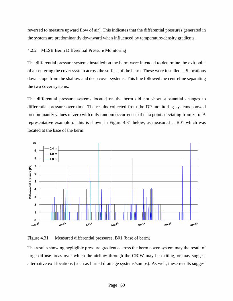
Page | 60
reversed to measure upward flow of air). This indicates that the differential pressures generated in
the system are predominantly downward when influenced by temperature/density gradients.
4.2.2 MLSB Berm Differential Pressure Monitoring
The differential pressure systems installed on the berm were intended to determine the exit point
of air entering the cover system across the surface of the berm. These were installed at 5 locations
down slope from the shallow and deep cover systems. This line followed the centreline separating
the two cover systems.
The differential pressure systems located on the berm did not show substantial changes to
differential pressure over time. The results collected from the DP monitoring systems showed
predominantly values of zero with only random occurrences of data points deviating from zero. A
representative example of this is shown in Figure 4.31 below, as measured at B01 which was
located at the base of the berm.
Figure 4.31 Measured differential pressures, B01 (base of berm)
The results showing negligible pressure gradients across the berm cover system may the result of
large diffuse areas over which the airflow through the CBIW may be exiting, or may suggest
alternative exit locations (such as buried drainage systems/sumps). As well, these results suggest
0
1
2
3
4
5
6
7
8
9
10
Dif
fere
nti
al P
ress
ure
(P
a)
0.4 m
1.0 m
2.0 m
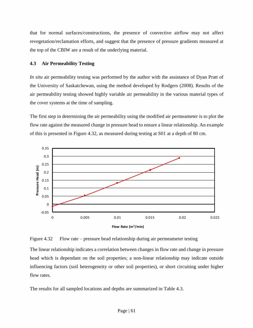
Page | 61
that for normal surfaces/constructions, the presence of convective airflow may not affect
revegetation/reclamation efforts, and suggest that the presence of pressure gradients measured at
the top of the CBIW are a result of the underlying material.
4.3 Air Permeability Testing
In situ air permeability testing was performed by the author with the assistance of Dyan Pratt of
the University of Saskatchewan, using the method developed by Rodgers (2008). Results of the
air permeability testing showed highly variable air permeability in the various material types of
the cover systems at the time of sampling.
The first step in determining the air permeability using the modified air permeameter is to plot the
flow rate against the measured change in pressure head to ensure a linear relationship. An example
of this is presented in Figure 4.32, as measured during testing at S01 at a depth of 80 cm.
Figure 4.32 Flow rate – pressure head relationship during air permeameter testing
The linear relationship indicates a correlation between changes in flow rate and change in pressure
head which is dependant on the soil properties; a non-linear relationship may indicate outside
influencing factors (soil heterogeneity or other soil properties), or short circuiting under higher
flow rates.
The results for all sampled locations and depths are summarized in Table 4.3.
-0.05
0
0.05
0.1
0.15
0.2
0.25
0.3
0.35
0 0.005 0.01 0.015 0.02 0.025
Pre
ssu
re H
ead
(m
)
Flow Rate (m3/min)

Page | 62
Table 4.3
Measured Intrinsic Air Permeability by Author (Sept, 2012)
Test Depth Average Air
Conductivity (m/s)
Average Intrinsic
Permeability (m2)
Shallow Cover
System
30 cm 4.1 x 10⁻⁵ 7.1 x 10⁻¹¹
80 cm 4.3 x 10⁻⁵ 6.7 x 10⁻¹¹
Deep Cover
System
30 cm 2.3 x 10⁻⁴ 3.8 x 10⁻¹⁰
80 cm 3.9 x 10⁻⁴ 6.5 x 10⁻¹⁰
110 cm 9.1 x 10⁻⁵ 1.5 x 10⁻¹⁰
The results in Table 4-1 are comparable to the average air permeability measurements made by
Rodgers (2008), as shown in Table 4.4, although the intrinsic air permeability of the cover systems
does appear to have decreased slightly since the testing carried out by Rodgers (2008). This
decrease in intrinsic permeability may be due to variation in methods used to conduct the tests, or
may be due to a change in the soil structure due to variable environmental conditions.
Table 4.4
Measured Air Permeability by Rodgers (2006)
Test Depth Trial 1 (m2) Trial 2 (m2) Trial 3 (m2)
10 cm 1.2 x 10⁻¹⁰ 1.8 x 10⁻¹⁰ 3.7 x 10⁻¹¹
20 cm 1.0 x 10⁻¹⁰ 2.5 x 10⁻¹⁰ 6.9 x 10⁻¹¹
30 cm 1.0 x 10⁻¹⁰ 2.8 x 10⁻¹⁰ 7.1 x 10⁻¹¹
40 cm 1.4 x 10⁻¹⁰ 3.6 x 10⁻¹⁰ 8.0 x 10⁻¹¹
The measured intrinsic permeability is independent of the VWC of the soil, however, the effective
air conductivity is going to be heavily influenced by the water content of the soil, as water within
the void space and higher effective saturation will limit the airflow in the system. If there is a high
presence of macropores, then air conductivity is less affected by moisture in the soil. This presents
a unique challenge when considering the air permeability and airflow potential of a reclamation
cover system, as the relative air permeability will change with changes in water content. A
combination of numerical modelling and intensive field investigation could determine a dynamic
air permeability for the site, however, this was outside the scope of this thesis.
4.4 Visual Observations Noted in the Field
Visual observations of the condition of the covers were made and recorded during regular site
visits were noted and recorded. One of the most striking observations was the presence of large
and deep surface cracks in the cover system across both the deep and shallow cover systems;

Page | 63
however, these were more prevalent on the shallow cover system (Figure 4.33). In many cases,
these surface cracks extended greater than 25 cm into the ground. The cracks would provide a
preferential pathway by which infiltrating water might bypass the cover system and enter the
underlying coke. If sufficient pathways exist at the cover systems, the result could be a water
movement pathway not currently covered by the standard water balance approach, and thus, would
affect the results. They would also provide high permeability flow paths for airflow. The effect of
these cracks on potential air movements across the cover system was not monitored and represents
a potential research opportunity.
Figure 4.33 Example of deep and wide surface cracking at the shallow cover system.
It was also noted that several areas of the cover system had begun to show loss of the surficial
peat, resulting in exposure of the underlying, lower hydraulic conductivity till. This loss in peat
may have been due to erosion by wind or water. In spite of this low hydraulic conductivity surface,
little to no ponding on the cover surface was not observed following heavy rainfalls consisting of
over 70 mm over four days in early June, 2013, and over 30 mm over two days at the end of May,
2013 and May 2014. This suggests that either runoff was occurring or that the surface cracks
provided for rapid infiltration of water in and possibly through the covers.

Page | 64
Each of the cover systems showed a substantial decrease in thickness of the peat layer. The peat
layer provides an important control on the water balance of the cover by allowing large
precipitation events to infiltrate and be stored so that the water can be released more slowly to the
underlying till layer.

Page | 65
Chapter 5
Analysis
The cover monitoring data, along with the field measurements of air-permeability and air pressure
will be used in this chapter to develop more quantitative interpretations of the water balance for
each of the covers as well as the magnitude of convective airflow. Daily and growing season water
balances were calculated for both covers for 2006 to 2014. These water balances are used to
identify if there is drying of the covers beyond that associated with normal evapotranspiration
and/or drainage. Estimates of airflow across the cover system as a function of time are used to
evaluate whether these airflow rates are sufficient to influence the water balance of the system.
5.1 Water Balances
5.1.1 Shallow Cover System
Actual evapotranspiration (AET) rates at the shallow cover system, calculated using the method
outlined in Section 2.8, are presented in Figures 5-1 through 5-9 for the years 2006 through 2014.
Included in each figure is a volume of water referred to as an “Additional Water Removal Process”
(AWR). This is the volume of water that would have to be removed to close the water balance for
the cover based on the conventional estimates of the water balance components. It will be used as
a semi-quantitative measurement of additional water losses not accounted for in the water balance
method outline in Section 2-5. In reality, visual observations of cracking suggest that the majority
of AWR is likely a component of net percolation (NP) as a result of bypass flow, however, this
could not be confirmed utilizing instrumentation in this thesis.
The AET/PET ratio was calculated using Equation 2.8 based on the measured volumetric water
contents (VWC). The values of field capacity (FC) and wilting point (WP) were taken from
published values as presented in Shurniak (2003) and summarized in Table 5.1.
Table 5.1
Summary of Cover System Material Properties
Cover System Component FC
(cm3/cm3)
WP
(cm3/cm3)
AWHC
(mm)
Shallow Cover Peat 0.3 0.20 20
Shallow Cover Till 0.35 0.21 28
Deep Cover Peat 0.30 0.20 25

Page | 66
Deep Cover Till 0.35 0.21 98
Similar studies were carried out at SCL 30-dump by Huang et al. (2015), using similar cover
system materials. The field capacity and wilting point of the material used in their study were 0.37
and 0.178, respectively. This shows good correlation to those values measured by Shurniak (2003).
The calculated and measured changes in storage for 2006 (Fig. 5-1) are similar with only minor
differences. This indicates that conventional estimates of AET and drainage are providing a
reasonable description of the water balance for this cover. The average AET:PET ratio during the
2006 field season was found to be 0.4, with the ratio falling to 0 during an extended dry period
when VWC dropped below the wilting point. It is interesting to note that the AWR for 2006 is
relatively low (e.g. ~ 50 mm) and appears to develop when there is a large precipitation event (e.g.
early spring or July 2006). This is likely water lost from storage as a result of drainage/bypass
flow.
Figure 5.1 Water balance for Shallow Cover System, 2006 monitoring year.
-100
0
100
200
300
400
500
600
700
800
Sto
rag
e (
mm
)
Cumulative PET
Cumulative Precipitation
AET
Calculated Storage
Measured Storage - CS616
Additional Water Removal Process

Page | 67
In subsequent years (2007-2014) the calculated AET:PET ratios become much lower than in 2006
during key evaporation months of June through August (e.g. 0.1 – 0.2). This occurs because the
VWC within the shallow cover remains near or below the wilting point through much of the
growing season from 2007 to 2014. These lower values of AET require that higher AWR volumes
are required to close the water balance increase. The increases in AWR during rapid increases in
precipitation likely reflect losses from rapid drainage; however, there are still ongoing increases
in AWR even during periods with smaller precipitation events. It is interesting to note that the
volume of AWR over the growing season was generally between 200 – 300 mm/year, and was
roughly 60-75% of the available precipitation. The volume of AWR for each monitoring year is
presented in Table 5.2, while the water balances for each monitoring year (2007 through 2014) at
the shallow cover system are shown in Figure 5.2 through Figure 5.9.
Figure 5.2 Water balance for Shallow Cover System, 2007 monitoring year.
-100
0
100
200
300
400
500
600
700
800
Sto
rag
e (
mm
)
Cumulative PET
Cumulative Precipitation
AET
Calculated Storage
Measured Storage - CS616
Additional water Removal Process

Page | 68
Figure 5.3 Water balance for Shallow Cover System, 2008 monitoring year.
-100
0
100
200
300
400
500
600
700S
tora
ge
(m
m)
Cumulative PET
Cumulative Precipitation
AET
Calculated Storage
Measured Storage - CS616
Additional Water Removal Process

Page | 69
Figure 5.4 Water balance for Shallow Cover System, 2009 monitoring year.
-100
0
100
200
300
400
500
600
700S
tora
ge
(m
m)
Cumulative PET
Cumulative Precipitation
AET
Calculated Storage
Measured Storage - CS616
Additional Water Removal Process

Page | 70
Figure 5.5 Water balance for Shallow Cover System, 2010 monitoring year.
-100
0
100
200
300
400
500
600
700S
tora
ge
(m
m)
Cumulative PET
Cumulative Precipitation
AET
Calculated Storage
Measured Storage - CS616
Additional Water Removal Process

Page | 71
Figure 5.6 Water balance for Shallow Cover System, 2011 monitoring year.
-100
0
100
200
300
400
500
600
700S
tora
ge
(m
m)
Cumulative PET
Cumulative Precipitation
AET
Calculated Storage
Measured Storage - CS616
Additional Water Removal Process

Page | 72
Figure 5.7 Water balance for Shallow Cover System, 2012 monitoring year.
-100
0
100
200
300
400
500
600
700S
tora
ge
(m
m)
Cumulative PET
Cumulative Precipitation
AET
Calculated Storage
Measured Storage - CS616
Additional Water Removal Process

Page | 73
Figure 5.8 Water balance for Shallow Cover System, 2013 monitoring year.
-100
0
100
200
300
400
500
600
700S
tora
ge
(m
m)
Cumulative PET
Cumulative Precipitation
Measured Storage - CS616
AET
Calculated Storage
Additional Water Removal Process

Page | 74
Figure 5.9 Water balance for Shallow Cover System, 2014 monitoring year.
-100
0
100
200
300
400
500
600
700S
tora
ge
(m
m)
Cumulative PET
Cumulative Precipitation
AET
Calculated Storage
Measured Storage - CS616
Additional Water Removal Process

Page | 75
Table 5.2 shows that the additional water removal (AWR) in the water balance formulation for the
Shallow Cover System as a function of the PET and precipitation which occurred at the site.
Table 5.2
Moisture Loss Not Accounted by Water Balance – Shallow Cover System
Year Total AWR
(mm)
Total Precipitation
(mm)
Total PET (mm)
AWR as Percentage of
Precipitation (%)
AWR as Percentage of
PET (%)
2006 106 332 692 32 15
2007 218 361 675 60 32
2008 271 392 596 69 45
2009 211 272 608 78 35
2010 195 307 632 64 31
2011 200 265 632 75 32
2012 305 422 613 72 50
2013 309 394 634 78 49
2014 205 341 603 60 34
The volume of AWR represents approximately 60-75% of precipitation in all monitoring years
save for 2006. The possible causes of this water loss are runoff, net percolation (particularly that
associated with preferential flow through fractures or macropores), or enhanced drying. The flat
topography of the cover and the lack of evidence of ponded conditions suggests that runoff is
unlikely. This suggests that the additional water loss is either the result of increased net percolation
as a result of flow through the macropores or the result of enhanced drying or both.
5.1.2 Deep Cover System
Unlike the shallow cover system, the deep cover system never showed a monitoring year in which
the calculated and measured storage were a good match without including a factor to account for
AWR. Figures 5-10 through 5-18 present the water balances obtained for 2006 through 2014. The
volume of AWR for each year as presented in Table 5-2 shows that the AWR for the deep cover
ranged from 140 to 293 mm/year, which is somewhat less than the AWR for the shallow cover.

Page | 76
Figure 5.10 Water balance for Deep Cover System, 2006 monitoring year.
-100
0
100
200
300
400
500
600
700
800S
tora
ge
(m
m)
Cumulative PET
Cumulative Precipitation
AET
Calculated Change in Storage
Measured Change in Storage - CS616
Additional Water Removal Process

Page | 77
Figure 5.11 Water balance for Deep Cover System, 2007 monitoring year.
-100
0
100
200
300
400
500
600
700
800S
tora
ge
(m
m)
Cumulative PET
Cumulative Precipitation
AET
Calculated Change in Storage
Measured Change in Storage - CS616
Additional Water Removal Process

Page | 78
Figure 5.12 Water balance for Deep Cover System, 2008 monitoring year.
-100
0
100
200
300
400
500
600
700
800S
tora
ge
(m
m)
Cumulative PET
Cumulative Precipitation
AET
Calculated Change in Storage
Measured Change in Storage - CS616
Additional Moisture Removal Process

Page | 79
Figure 5.13 Water balance for Deep Cover System, 2009 monitoring year.
-100
0
100
200
300
400
500
600
700
800S
tora
ge
(m
m)
Cumulative PET
Cumulative Precipitation
AET
Calculated Change in Storage
Measured Change in Storage - CS616
Additional Water Removal Process
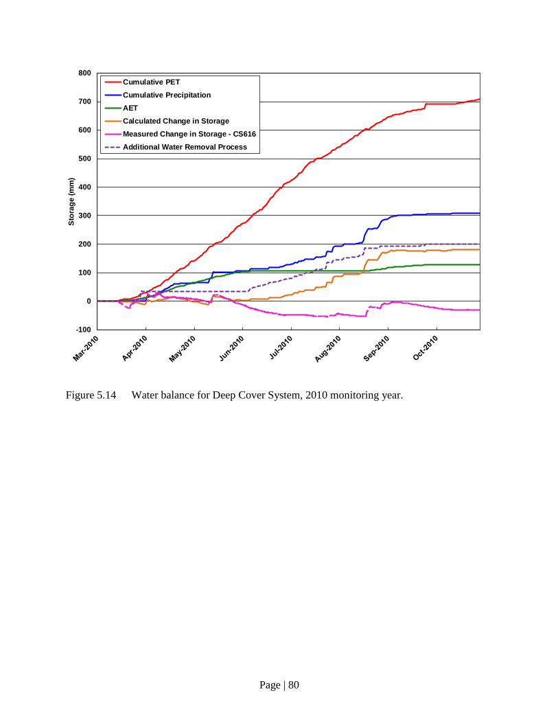
Page | 80
Figure 5.14 Water balance for Deep Cover System, 2010 monitoring year.
-100
0
100
200
300
400
500
600
700
800S
tora
ge
(m
m)
Cumulative PET
Cumulative Precipitation
AET
Calculated Change in Storage
Measured Change in Storage - CS616
Additional Water Removal Process

Page | 81
Figure 5.15 Water balance for Deep Cover System, 2011 monitoring year.
-100
0
100
200
300
400
500
600
700
800S
tora
ge
(m
m)
Cumulative PET
Cumulative Precipitation
AET
Calculated Change in Storage
Measured Change in Storage - CS616
Additional Water Removal Process

Page | 82
Figure 5.16 Water balance for Deep Cover System, 2012 monitoring year.
-100
0
100
200
300
400
500
600
700S
tora
ge
(m
m)
Cumulative PET
Cumulative Precipitation
AET
Calculated Change in Storage
Measured Change in Storage - CS616
Additional Water Removal Process

Page | 83
Figure 5.17 Water balance for Deep Cover System, 2013 monitoring year.
-100
0
100
200
300
400
500
600
700S
tora
ge
(m
m)
Cumulative PET
Cumulative Precipitation
AET
Calculated Change in Storage
Measured Change in Storage - CS616
Additional Water Removal Process

Page | 84
Figure 5.18 Water balance for Deep Cover System, 2014 monitoring year.
-100
0
100
200
300
400
500
600
700S
tora
ge
(m
m)
Cumulative PET
Cumulative Precipitation
AET
Calculated Change in Storage
Measured Change in Storage - CS616
Additional Water Removal Process

Page | 85
Table 5.3 shows that the additional water removal (AWR) in the water balance formulation for the
Deep Cover System as a function of the PET and precipitation which occurred at the site.
Table 5.3
Moisture Loss Not Accounted by Water Balance – Deep Cover Sytem
Year
Total AWR (mm)
Total Precipitation
(mm)
Total PET (mm)
AWR as Percentage of
Precipitation (%)
AWR as Percentage of
PET (%)
2006 140 341 692 41 20
2007 231 364 675 63 34
2008 293 392 596 75 49
2009 177 272 608 65 29
2010 201 307 632 65 32
2011 197 265 632 74 31
2012 239 424 613 56 39
2013 270 387 634 70 43
2014 215 328 603 60 36
Similar results comparing the AWR to the precipitation were observed at the Deep Cover System
in that 60-75% of all precipitation is lost to the AWR process and is not captured in the water
balance.
A comparison between the AWR measured at both the Shallow and Deep cover system is presented
in Figure 5.19. Generally speaking, the Shallow Cover System showed higher values for AWR as
compared to the Deep Cover System, however, both cover systems showed similar trends. It is
hypothesized that a larger volume of bypass flow is occurring at the shallow cover since casual
measurements of cracking was observed to occur to depths of 25 cm, which represents
approximately half the depth of the cover system but less than a quarter the depth of the deep cover
system. As a result, any excess water entering the crack system on the surface of the Shallow Cover
System would percolate/infiltrate more rapidly through the remaining cover system profile than at
the Deep Cover System. The observations of cracking at the surface of each cover system were
performed on a casual basis, and a more extensive crack survey may reveal deeper cracks which
penetrate the entirety of the Shallow Cover System. Other unaccounted moisture/water loss
streams may include runoff and percolation, which would be reflected in the AWR and were not
captured in the water balance monitoring equipment.

Page | 86
Figure 5.19 Comparison of AWR measured at Deep and Shallow Cover Systems
0
50
100
150
200
250
300
350
400
450
2005 2006 2007 2008 2009 2010 2011 2012 2013 2014 2015
Wa
ter
Flu
x (m
m)
Date
Shallow Cover AWR
Deep Cover AWR
Annual Precipitation
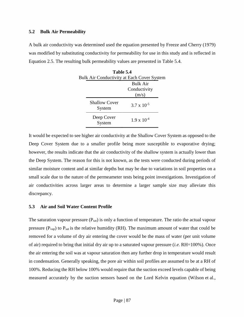
Page | 87
5.2 Bulk Air Permeability
A bulk air conductivity was determined used the equation presented by Freeze and Cherry (1979)
was modified by substituting conductivity for permeability for use in this study and is reflected in
Equation 2.5. The resulting bulk permeability values are presented in Table 5.4.
Table 5.4
Bulk Air Conductivity at Each Cover System
Bulk Air
Conductivity
(m/s)
Shallow Cover
System 3.7 x 10⁻⁵
Deep Cover
System 1.9 x 10⁻⁴
It would be expected to see higher air conductivity at the Shallow Cover System as opposed to the
Deep Cover System due to a smaller profile being more susceptible to evaporative drying;
however, the results indicate that the air conductivity of the shallow system is actually lower than
the Deep System. The reason for this is not known, as the tests were conducted during periods of
similar moisture content and at similar depths but may be due to variations in soil properties on a
small scale due to the nature of the permeameter tests being point investigations. Investigation of
air conductivities across larger areas to determine a larger sample size may alleviate this
discrepancy.
5.3 Air and Soil Water Content Profile
The saturation vapour pressure (Psat) is only a function of temperature. The ratio the actual vapour
pressure (Pvap) to Psat is the relative humidity (RH). The maximum amount of water that could be
removed for a volume of dry air entering the cover would be the mass of water (per unit volume
of air) required to bring that initial dry air up to a saturated vapour pressure (i.e. RH=100%). Once
the air entering the soil was at vapour saturation then any further drop in temperature would result
in condensation. Generally speaking, the pore air within soil profiles are assumed to be at a RH of
100%. Reducing the RH below 100% would require that the suction exceed levels capable of being
measured accurately by the suction sensors based on the Lord Kelvin equation (Wilson et al.,

Page | 88
1997). Representative values of saturation and actual vapour pressure can be calculated from the
in situ monitoring sensors (temperature and suction) from each cover system. Both cover systems
show development of suctions in the rooting zone which indicate moisture content falls below the
wilting point of the respective soil materials.
5.3.1 Ambient Air and Soil Air Moisture Availability
The ambient air properties were used in order to estimate the saturated vapour pressures using
Equation 3.1. This same method was used in combination with soil temperature profiles from
automated monitoring sensors to calculate the saturation vapour pressure in the soil voids.
The vapour pressure of the ambient air was determined using available temperature and RH data,
averaged on a daily basis. Relative humidity of the air in the soil voids was assumed to be 100%
due to measured suction values indicating lower than wilting point for the duration of the field
period. Using this information to determine RH, the actual vapour pressure of the soil can be
determined using Equation 3.2.
The moisture removal potential of a parcel of air passing through the cover system is dependent
on the difference between the saturated and actual vapour pressures of said parcel of air. Working
with these assumptions, the soil moisture availability for the shallow cover system and deep cover
system through the 2013 monitoring year was calculated by determining the difference between
the Psat of the air in soil voids, and the Pvap of the ambient air. The value for Psat in the cover systems
was calculated at the base of each cover system based on the measured temperature; this location
and method was selected due to uncertainty with calculation of RH from the soil suction sensors,
and to remove uncertainty with non-uniformity of the cover system moisture profile. This
difference represents the additional moisture required to bring the moisture conditions of the
ambient air to equilibrium with the air in the soil voids.
For example, on June 5, 2013 the average air temperature was 15.6oC with an average RH of 0.77,
which when used in conjunction with Equations 3.1 and Equation 3.2 results in a vapour
concentration in the air of 8.99 g/m3. In addition, the average soil temperature as measured by the
CS229 sensors was 18oC. The soil moisture availability at this temperature, calculated using
Equation 3.3 with the average soil temperature, showed that the water concentration in the air

Page | 89
within the soil voids was an average of 9.5 g/m3. The maximum available moisture for removal is
the difference between the ambient air vapour concentration and the saturated soil vapour
concentration; this would bring the two values into equilibrium. As such, in this example the
difference between the soil vapour concentration and ambient air concentration is approximately
0.5 g/m3.
The resulting moisture availability coupled with calculations of airflow presented in Section 5.5
can be used to determine the total moisture loss due to airflow across the system. The moisture
availability for the shallow and deep cover systems are presented in Figure 5.20 and Figure 5.21
for the 2013 monitoring years, respectively.
Figure 5.20 Shallow cover system moisture removal potential during 2013.
0.00
1.00
2.00
3.00
4.00
5.00
6.00
7.00
8.00
Mo
istu
re A
va
ila
bilit
y (g
/m³)
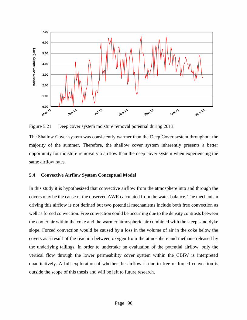
Page | 90
Figure 5.21 Deep cover system moisture removal potential during 2013.
The Shallow Cover system was consistently warmer than the Deep Cover system throughout the
majority of the summer. Therefore, the shallow cover system inherently presents a better
opportunity for moisture removal via airflow than the deep cover system when experiencing the
same airflow rates.
5.4 Convective Airflow System Conceptual Model
In this study it is hypothesized that convective airflow from the atmosphere into and through the
covers may be the cause of the observed AWR calculated from the water balance. The mechanism
driving this airflow is not defined but two potential mechanisms include both free convection as
well as forced convection. Free convection could be occurring due to the density contrasts between
the cooler air within the coke and the warmer atmospheric air combined with the steep sand dyke
slope. Forced convection would be caused by a loss in the volume of air in the coke below the
covers as a result of the reaction between oxygen from the atmosphere and methane released by
the underlying tailings. In order to undertake an evaluation of the potential airflow, only the
vertical flow through the lower permeability cover system within the CBIW is interpreted
quantitatively. A full exploration of whether the airflow is due to free or forced convection is
outside the scope of this thesis and will be left to future research.
0.00
1.00
2.00
3.00
4.00
5.00
6.00
7.00M
ois
ture
Av
aila
bilit
y (g
/m³)
Page | 91
Due to the fact that the differential pressure cycles coincide with the temperature cycle, it suggests
that the differential pressures and resultant airflow are linked to the temperature variations
(advective airflow) rather than chemical reactions (forced airflow). However, this does not
discredit the potential for forced airflow entirely, and also does not eliminate the possibility that
the temperature of the stored coke was unaffected by chemical reactions in the subsurface, and
further investigation is still warranted.
5.5 Calculation of Convective Airflow
The presence of actual airflow versus the theoretical presence based on temperature and density
gradients is heavily reliant on the soil air permeability. The permeability of the soil to air is lowest
in early summer due to a high soil VWC, and is greatest in late summer due to a low VWC as a
result of continual drying throughout the summer months. Due to the difficulties in determining
changes in the density profile within the column of air due to dynamic temperature and pressure
changes, the analysis of airflow was simplified as a preliminary evaluation for the potential for
airflow drying. The analysis is based on the measured values of differential pressure presented in
Section 4.2, which is taken at a constant elevation assuming that the density profile between the
measurement points (surface and subsurface) is not affecting flow.
5.5.1 Estimate of Airflow Rates
Using the differential pressure data shown in Section 4.2 in conjunction with the average bulk air
permeability determined in Section 4.3, an estimate of airflow rates through the cover system can
be calculated for each differential pressure monitoring location using Equation 2.3. It should be
noted that the soil VWC is measured at the centre of each cover system (S02 and D02), whereas
the differential pressure is measured at three locations. For the purposes of this calculation, it is
assumed that the measured VWC at the centre of the cover systems represent the water content
distribution across the entire cover system. It is likely that the moisture conditions varied in space
across the cover system, and as such, the air permeability may not have been accurately represented
at the outlying S01, S03, D01, and D03 monitoring locations.
For example, using 2.3, an assumed bulk air conductivity for the shallow cover system of 3.7 x 10-
5 m2, a density of air of 1.19 kg/m3, a barometric pressure of 97.0 kPa, ambient temperature of

Page | 92
20oC, ambient RH of 70%, a vertical distance of 0.3 m, and a differential pressure of 10 Pa as
follows:
fg = 3.7 𝑥 10−5𝑚
𝑠∗ (
10 𝑃𝑎
0.3 m ∗ 9.81m𝑠2 ∗ 1.19
kg𝑚3
) = 1.07 𝑥 10−4𝑚
𝑠
results in a calculated airflow rate of 1.07 x 10⁻⁴ m/s, or when applied over an area of 1 m2,
9.21 m3/day.
The results for the 2013 monitoring year are shown in Figure 5.22 and Figure 5.23 for the shallow
cover system and deep cover system, respectively.
Figure 5.22 Calculated shallow cover system downward airflow rates, 2013
1.00E-04
1.00E-03
1.00E-02
1.00E-01
1.00E+00
1.00E+01
1.00E+02
Air
flo
w th
rou
gh
Co
ve
r S
ys
tem
(m
/da
y)
S01 Airflow
S02 Airflow
S03 Airflow

Page | 93
Figure 5.23 Calculated deep cover system downward airflow rates, 2013
Under similar differential pressures/permeabilities relative to their monitored depths, the
calculated airflow rates at both the deep and shallow cover systems should be similar. However,
the Deep Cover System showed a higher calculated airflow rate due to a higher bulk permeability
than the Shallow Cover System. A sensitivity analysis is presented in Section 5.6 to investigate
the effects of higher air conductivities on both cover systems and to determine the effects on
potential moisture removal under variable conditions.
5.5.2 Airflow Induced Moisture Removal
In order to calculate the potential moisture removal via airflow, it was necessary to assume
instantaneous equilibrium of soil moisture to air moisture within the soil voids, and that a
downward moving parcel of air was unsaturated at the point of entering the cover system, and was
saturated following departure from the voids of the cover system (difference between saturated
vapour pressure and actual vapour pressure is representative of soil moisture removal). This
1.00E-03
1.00E-02
1.00E-01
1.00E+00
1.00E+01
1.00E+02A
irfl
ow
th
rou
gh
Co
ve
r S
ys
tem
(m
/da
y)
D01 Airflow
D02 Airflow
D03 Airflow
Note: D03 airflow calculation used 2 m sensor as opposed to 1.1 m sensor due to sensor failure.

Page | 94
assumption, although potentially not truly representative of field conditions, would allow for
estimation of the maximum moisture removal due to airflow across the cover systems.
The calculated maximum potential moisture removal rates were based on the calculated airflow
and the moisture removal potential previously discussed in Sections 5.5.1 and 5.3.1, respectively.
These values are calculated based on the assumed conditions within the cover system and the
assumed properties of the air used in calculating the airflow and moisture removal potential and
can be found in Figure 5.24. The estimated moisture removal rate is calculated as shown in
Equation 3.3. The results are converted into units of millimetres following the calculation to
maintain consistency with the units in the water balances. The results are presented in Figure 5.24
and Figure 5.25 for the 2013 monitoring year for the shallow cover system and deep cover system,
receptively.
Figure 5.24 Calculated cumulative maximum moisture removal potential using calculated
airflow and moisture removal potential – shallow cover system
1.00E-06
1.00E-05
1.00E-04
1.00E-03
1.00E-02
1.00E-01
1.00E+00
Air
flo
w In
du
ce
d M
ois
ture
Lo
ss
(m
m)
S01 Airflow
S02 Airflow
S03 Airflow

Page | 95
Figure 5.25 Calculated cumulative maximum moisture removal potential using calculated
airflow and moisture removal potential – deep cover system
As can be seen, the majority of moisture removal from both the shallow and deep cover systems
occurs in June/July, while at the deep cover system it occurs in August/September. However, due
to the low permeability of the cover system resulting in low airflow rates, the overall moisture
removal rates were several orders of magnitude lower than the overall moisture availability in the
system. The overall low airflow rates and low potential for moisture losses associated with the
airflow across each cover system indicate that the hypothesis that convective airflow is the primary
cause of the enhanced drying of the cover systems is proven false, and the unaccounted moisture
loss in each system is likely attributed to another outside influencing factor. Alternatively, the
convection rates may be underestimated as a result of limited permeability data.
5.6 Convective Drying Sensitivity Study
An analysis was performed which increased the measured permeability by two orders of magnitude
(100 multiplication factor) and three orders of magnitude (1000 multiplication factor) to determine
the effect on the moisture removal rates as they pertained to the water balance. This allows us to
1.00E-06
1.00E-04
1.00E-02
1.00E+00A
irfl
ow
In
du
ce
d M
ois
ture
Lo
ss
(m
m)
D01 Airflow
D02 Airflow
D03 Airflow

Page | 96
determine what airflow rates would be required to cause the increase in moisture removal observed
at each cover system.
In both cases of the shallow cover system and deep cover system, an increase in permeability of
three orders of magnitude is unlikely and represents a large deviation from the conditions observed
during field observations; however, the analysis is intended to represent what is required for
convective moisture removal to have a significant effect on the cover system moisture conditions.
Given the highly variable moisture content of the cover system, a variable permeability is highly
likely throughout the summer, and may result in additional losses from the cover system depending
on local weather conditions. These additional losses when considering a variable permeability,
coupled with increase percolation due to macro-pore formation, or additional runoff not accounted
for in the water balance may contribute to a more accurate water balance formulation.
The results of the water balance formulation considering the increase in average permeability are
shown in Figure 5.26 and Figure 5.27 for the shallow cover system and deep cover system
respectively.
Figure 5.26 Water Storage assuming increased permeability at shallow cover system, 2013
monitoring year
-100
0
100
200
300
400
500
600
700
Sto
rag
e (
mm
)
Measured Storage - CS616
Calculated Storage
Conductivity Increased by Two Orders Magnitude (100x)
Conductivity Increased by Three Orders Magnitude (1000x)

Page | 97
Figure 5.27 Water storage assuming increased permeability at deep cover system, 2013
monitoring year
Increasing the hypothetical permeability of each cover system by two orders of magnitude did not
increase airflow rates sufficiently to have a substantial impact on moisture removal rates, and thus
did little to affect the water balance.
At the shallow cover system, an increase of three orders of magnitude, or equivalent to increasing
the permeability by 1,000 started to show calculated storage values decrease towards the measured
storage values, indicating that further increases in permeability would be required to further
calibrate the water balance. The general shape and trends of the calculated storage using a three
order of magnitude increase on the permeability value matches that of the calculated storage curve,
and it is likely that if the hypothetical permeability were increased by another 1,000, convergence
of the two curves would be likely.
At the deep cover system, a three order of magnitude increase to the measured permeability value
resulted in a near match of the calculated storage and measured storage values until the end of
July. At this point, the increased permeability resulted in airflow rates which removed more
moisture than was required to allow for convergence of the measured and calculated storage
values.
-200
-100
0
100
200
300
400S
tora
ge
(m
m)
Measured Storage - CS616
Calculated Storage
Conductivity Increased Two Orders Magnitude (100x)
Conductivity Increased Three Orders Magnitude (1000x)

Page | 98
The broad application of a standard increase in permeability does not represent true conditions in
the field and does not account for changes in rainfall and soil moisture throughout the summer. In
addition, daily permeability values will change as a result of changes in moisture conditions, thus
further complicating the analysis.
A sensitivity analysis on the bypass/runoff during major storm events was carried out in order to
investigate the effect the potential increased infiltration/bypass flow may have on the water balance
formulation. Included in this sensitivity analysis was an increase in the permeability of the cover
system by a factor of 400 to determine what airflow rates would be required in order to remove
sufficient moisture to “close” the water balance formulation.
It was noted that changes in soil VWC coincided with major storm events (i.e. those exceeding
5 mm in a 24-hour period), however, minor storm events (i.e. those less than 5 mm in a 24-hour
period) had minor to zero impact on the VWC in the upper 30 cm of the soil profile. This is shown
by the comparison of changes in soil moisture content to precipitation events (Figure 5.28).
Figure 5.28 Precipitation effects on soil moisture in Shallow Cover System rooting zone.
The major storm events were analyzed on a case by case basis, and the relative changes to soil
VWC as a percentage of total rainfall are presented in Table 5.5.
0
3
6
9
12
15
18
21
24
0
5
10
15
20
25
30
35
40
Da
ily
Ch
an
ge
in S
tora
ge
(m
m)
Da
ily
Pre
cip
ita
tio
n (
mm
)
Daily Precipitation Daily Change in Storage

Page | 99
Table 5.5
Comparison of Change in Storage to Precipitation at the Shallow Cover System
Storm Event Date Range Change in VWC versus
Precipitation (%)
June 5 through June 13, 2013 32.3
June 26 through June 28, 2013 15.2
July 4 through July 14, 2013 0
July 27 through July 31, 2013 35.3
August 25 through September 1, 2013 11.9
Based on the above information, the sensitivity analysis was carried out assuming that for all storm
events aside from those listed above, any precipitation in excess of that already accounted for in
the water balance will bypass the cover system through other processes (macropore flow or runoff),
while for those storm events listed above the bypass rate will be calculated using the fractions
listed in Table 5.4.
The resulting water balance formulation including the increased airflow capacity is presented in
Figure 5.29.
Figure 5.29 Increased infiltration and airflow rates sensitivity analysis – shallow cover system.
The results seen in Figure 5.29 show that the large rainfall events had a substantial impact on the
overall water balance; the blue line representing the newly calculated storage minus the bypass
-100
0
100
200
300
400
500
600
700
Sto
rag
e (
mm
)
Measured Storage - CS616
Calculated Storage w/Bypass
Bypass Flow
Calculated Storage w/ Bypass and 400xIncreased Conductivity

Page | 100
flow shows a much better correlation with the measured storage. In addition, by increasing the
permeability of the cover system by a factor of 400 in conjunction with the new consideration for
bypass water flow, it allows for a good correlation of calculated storage with the measured storage,
indicating that the airflow at this permeability condition would be sufficient enough to have an
impact on the moisture condition of the cover system. An increase in permeability of this level is
not entirely unfeasible, as the cracking observed in the cover system would allow for such an
increase; in addition, variations in cover system moisture content may allow for increased
permeability throughout the summer season; a detailed permeability monitoring system would be
able to verify this hypothesis.

Page | 101
Chapter 6
Summary and Recommendations
Soil covers at Syncrude Canada’s Coke Beach Instrumented Watershed have appeared to undergo
greater water losses than can be accounted for from calculations of AET since cover construction
in 2004. These additional water losses appear to also be linked to drying of the cover to levels
below water contents associated with wilting point. Preliminary investigations hypothesized that
the enhanced drying effect was a result of convective airflow of dry atmospheric air in through the
covers, causing enhanced evaporation. As outlined in Chapter 1, the purpose of this investigation
was to
• Design and implement a field monitoring system to determine the presence, or lack there-
of, of this downward airflow cycle and to account for the changes in the internal moisture
storage of the cover system.
• Design and install additional field instrumentation to identify the presence and magnitude
of airflow through the cover profiles at the CBIW. This instrumentation is to include
differential air pressure and barometric pressure monitoring.
The field data was subsequently analyzed using a variety of analytical methods to assess the
potential for convective airflow and subsequent enhanced water removal from the cover systems.
6.1 Cover System Instrumentation.
Watershed monitoring instrumentation was installed by O’Kane Consultants Inc. in 2004 as part
of the initial cover system construction. This included:
• Meteorological monitoring instrumentation which measured precipitation (rainfall),
relative humidity, temperature, wind speed, and net radiation. This data was compared and
verified with the Fort McMurray International Airport data.
• Soil moisture content using CS616 time domain reflectometry probes. Water contents
measured in the soil cover systems were measured adequately during the field observation
period, and there was a sufficient amount of data to verify the moisture conditions in each
of the cover systems. The water content sensors proved to be a valuable tool to assess the

Page | 102
water balance and in-system moisture transfer processes. Using the moisture content
sensors in conjunction with meteorological sensors, a detailed water balance was
generated, the moisture removal potential of migrating airflow was calculated, and the
impact of the enhanced evaporation from was pinpointed throughout all monitoring years.
• Soil suction and temperature was measured using CS229 thermal conductivity sensors. The
soil matric potentials measured by these sensors were utilized to calculate soil RH which
proved to be a vital component of calculating the moisture removal potential of air moving
across the cover system. In addition, the temperatures measured provided a valuable tool
to present a conceptual understanding of airflow dynamics in the subsurface and
contributed to calculating the density of air in the subsurface which was utilized to calculate
a density gradient across the cover system and thus relative direction of airflow movement.
In order to quantify the potential for airflow across the cover system, the author of this thesis
installed the following additional instrumentation:
• The barometric pressure monitor installed by the author recorded data on a regular basis
and was successfully used in the investigation. The sensor proved to be a valuable tool to
benchmark the ambient and subsurface air densities.
• Differential pressure sensors and dataloggers which tracked the difference in pressure
gradients from the ambient atmosphere relative to the subsurface. In total, 18 sensors were
installed at the cover system; however, in reviewing the data the most valuable results
proved to be from the sensors installed at 2 m below the surface of the cover systems. It
was this sensor which coincided with the air mass representative of the deep temperature
gradients and thus driving force behind any air temperature driven movement in the system.
When using this sensor coupled with the soil monitoring stations installed by OKC the
airflow across the cover system was determined successfully and applied to the water
balance via moisture transfer processes.
• Despite being successful at measuring uni-directional differential pressure, the differential
pressure monitoring system was limited in that it could not measure upward movement (bi-
directional) airflow. In order to investigate the potential for bi-directional flow, the
differential pressure sensors were reversed in 2014, and were only capable of measuring

Page | 103
upward airflow gradients. During this period, minimal pressure gradients indicated upward
airflow, and as such, it is not likely that reversal of flow conditions occurred frequently.
However, in order to improve similar monitoring systems in the future, bi-directional
sensors would be ideal, and would allow for continuous monitoring of flow in both
directions.
• Measured differential pressures in 2013 generally showed diurnal trends, with little to no
differential pressure measured at night (DP=0 Pa), while during the day, negative
differential pressures varied from as low as 0 Pa to over 60 Pa.
• Measured differential pressures in 2014 were limited to only a few instances of values not
equivalent to 0; however, several of these values did reach differential pressures of 60 Pa
at instantaneous points in time. That is rather than a gradual increase, point measurements
of high differential pressures were measured. These may be attributed to sensor error due
to the lack of correlation with preceding measurements.
• Air permeability testing was successfully performed with results comparing to previously
measured values determined at the point of development of the air permeameter. The
method developed by Rodgers (2008) was successfully adapted to the AMS International
sampling system in conjunction with measurements from the differential pressure sensors
to measure air permeability’s at both cover systems. When coupling the measured data with
known VWC values at the time of measurement, a broad, full scale volumetric air
content/permeability function was calculated and applied to airflow calculations. This
allowed for dynamic calculations of airflow throughout the 2013 monitoring season and
contributed to the successful determination of airflow enhanced moisture removal from the
cover system.
• Air permeability measured as part of this thesis correlate with previous measurements
made by Rodgers (2008) at the same cover system. Measured permeabilities at the shallow
and deep cover system were found to be in the range of 10-10 to 10-11 m2. The permeability
measured at a depth of 30 cm in the shallow cover was approximately 1 order of magnitude
lower than the other measurements made at the same time at other locations, as well as
when compared to Rodgers (2008). This result may have been due to differences in soil
water content at the time of measurement, but also shows the wide range of permeabilities

Page | 104
across the cover system. A detailed investigation of variable permeabilities would allow
for the convective airflow model to be refined and more accurately calculate airflow rates.
6.2 Field Measurements Assessing Airflow across Cover Systems
The differential pressure sensors installed on the cover systems were successfully used to measure
pressure gradients across the cover system and were vital in measuring field air permeability.
Compared to published papers and case studies, the measured differential pressures at both cover
systems indicated a high potential for a convective airflow system to exist due to the presence of
high differential pressures across a relatively small vertical distance.
Airflow rates across the cover system were then calculated using a modified version of Darcy’s
law combined with a dynamic cover system permeability calculated from field testing and field
measurements. Airflow rates occurred across the cover system throughout the year at both cover
systems, however, when combined with moisture availability in the soil it was shown that the
airflow rates were insufficient to cause any effective enhanced moisture removal which would
explain excess moisture losses in either cover system. The measured airflow rates at the shallow
cover system and the deep cover system showed similarities, in that daily airflow rates varied
between 0 m3/day to approximately 50 m3/day at peak flow periods; however average airflow rates
at each cover system and at all monitoring points was between 1 m3/day and 2 m3/day. The low
average airflow rates proved to be insufficient to remove water from the cover system when using
the constant air conductivity value measured for each cover system. However, application of a
dynamic air conductivity based on measured suctions and VWC may affect calculated airflow rates
substantially and would be more representative of the dynamic water content within the cover
system throughout the year.
The lack of evidence for convective airflow affecting moisture in the cover systems suggests that
there is an alternative process occurring within the systems which is affecting the moisture
availability in the soil. This is proven by the fact that the water balances for the systems do not
account for a large portion of moisture removal required to match calculated storage and measured
storage values.

Page | 105
Based on this conclusion, there may be another process occurring which is causing the enhanced
drying of each cover system. The presence of forced convection via the occurrence of chemical
reactions of the underlying coke with oxygen rich atmospheric air may be contributing to the
enhanced drying being observed. Although temperature/density gradient data indicates that the
advective airflow process is possible, it does not fully discredit the presence of forced convection.
Further research at the site will be required to determine the cause of this enhanced drying.
6.3 Research Refinements and Future Research Potential
The water balance in both cases of the shallow and deep cover systems could be further refined to
be more inclusive of runoff, however, the purpose of this thesis is to prove the presence of
convective airflow. It was proven that convective airflow within the system is likely not a
contributing factor to moisture losses unless a more thorough study of cover system permeability
rates indicates that a larger permeability is present than those which were measured during this
thesis. This was determined effectively using in situ differential pressure sensors. With very low
instrumentation costs, the differential pressure was measured and combined with standard cover
system monitoring equipment to provide a more comprehensive understanding of water flow
processes in an otherwise complex system. The lack of evidence for convective airflow enhanced
moisture removal can be used to remove one possibly cause of the enhanced moisture removal
processes seen at the cover systems. The system can be used effectively at other locations to
perform similar analyses and may be used to measure moisture removal as a result of airflow
processes effectively at locations where cover systems are constructed with more permeable
materials such as sand or gravel. In future usage, the airflow monitoring system can be further
refined with the inclusion of more research opportunities:
• Other contributing processes to the airflow in the system, such as chemical reactions with
the stored coke (oxygen consumption processes). This may be performed by measuring gas
chemistry profiles in the subsurface to determine oxidation/degradation rates of various
known constituents (e.g. Methane, oxygen) and use the variable concentrations to
determine potential for convective cycles via density gradients.

Page | 106
• Inclusion of bi-directional differential pressure sensors at multiple locations across the
cover system to account for the potential of air rising through the cover systems as well as
the potential for downward migration simultaneously.
• Monitoring of RH in soil voids continuously using sensors specific to that purpose; this
would alleviate issues with the current suction sensors and the limited range available using
these sensors for determination of RH.
• Development of a numerical modelling program to determine a daily change in
permeability due to soil moisture content affecting permeability of the soil to air will
further refine the conceptual model of convective airflow at the CBIW. Numerical
modelling will allow for inclusion of regular changes to soil VWC and the ability to
compare these changes to measured changes in the field. In addition, numerical modelling
will allow for variations in permeability as a function of VWC, more accurately
representing the true variable nature both spatially and temporally of soil cover system
conditions. Drier periods would show higher permeability to soil, while periods seeing
more rainfall would show lower permeabilities.
• Measurements and regular monitoring of bulk air permeability across more locations on
the cover system to assess variable air conductivities as a function of spatial location and
the effect on potential airflow based on variable air conductivities. If a higher permeability
is measured across the cover system, this would lead support to the original hypothesis as
the pressure gradients are substantial enough to indicate the presence of airflow rates to
induce enhanced drying under higher permeability conditions.
The overall water balance method still shows a process for moisture removal that is not being
accounted for in using the current field instrumentation, inclusive of the now installed differential
pressure monitoring system. In order to more effectively monitor water movement in the system,
the following changes to field measurements can be made, and will assist with further research at
the project location:
• Inclusion of system to quantify runoff, interflow, and net percolation/flow bypass across
the cover systems to further refine water balance and capture moisture losses more
accurately, especially in the case of the deep cover system; and

Page | 107
• Vegetation surveys of the trees planted on the cover system to identify the extent of impact
the enhanced drying has had on the overall reclamation efforts.

Page | 108
REFERENCES
Amos, R., Ulrich Mayer, K., Bekins, B. Delin, G., Williams, R. (2005). Use of dissolved and
vapor-phase gases to investigate methanogenic degradation of petroleum hydrocarbon
contamination in the subsurface. Published in Water Resources Research, Vol. 41.
Arenson, L. U., Chen, J. F., Pham, H., & Sego, D. C. (2007). Laboratory Investigations On Air
Convection In Porous Media, (2006), 1836–1843.
Ball, B. C., & Schjønning, P. (2002). Methods of Soils Analysis Part 4 (pp. 1141 – 1158).
Madison, Al: Soil Science Society of America.
Barbour, S. (1998). The soil-water characteristic curve: a historical perspective. Canadian
Geotechnical Journal.
Bauters, T. W. ., Steenhuis, T. ., DiCarlo, D. ., Nieber, J. ., Dekker, L. ., Ritsema, C. Haverkamp,
R. (2000). Physics of water repellent soils. Journal of Hydrology, 231-232, 233–243.
doi:10.1016/S0022-1694(00)00197-9
Birkham, T. K., M. J. Hendry, and S. L. Barbour. "Advective and diffusive gas transport through
fractured sulfur blocks." Vadose Zone Journal 9.2 (2010): 451-461.
Birkham, T. K., Hendry, M. J., Barbour, S. L., & Lawrence, J. R. (2010). Controls and rates of
acid production in commercial-scale sulfur blocks. Journal of environmental quality,
39(3), 834-844.
Birkham, T. K., Hendry, M. J., Barbour, S. L., Carey, S. K., Lawrence, J. R., & Lewko, R.
(2011). Water flow and storage in fractured, unsaturated sulphur blocks. Canadian
Geotechnical Journal, 48(5), 810-825.
Brooks, K., Folliott, P. F., & Magner, P. A. (2013). Hydrology and the Management of
Watersheds (4e ed.). Ames, Iowa: Wiley-Blackwell Publishing.
Chin, D. A. (2006). Water Resources Engineering (2nd ed.). New Jersey: Pearson - Prentice
Hall.

Page | 109
Cumulative Environmental Land Management Association. (2006). Land Capability
Classification System for Forest Ecosystems (Vol. 1).
Doerr, S. H., Shakesby, R. a., & Walsh, R. P. D. (2000). Soil water repellency: its causes,
characteristics and hydro-geomorphological significance. Earth-Science Reviews, 51(1-
4), 33–65. doi:10.1016/S0012-8252(00)00011-8
da Silva, C., Vargas, E., Sracek, O. 2009. Modeling Multiphase REactive Transport in a Waste
Rock Pile with Convective Oxygen Supply. Vadoze Zone Journal 8:1038-1050.
Dunbar, R. B. (2009). Canada ’ s Oil Sands - A World-Scale Hydrocarbon Resource, (February).
Fenske, D. (2012). A study to evaluate the performance of reclamation soil covers placed over
an oil sands fluid coke deposit. Masters Thesis, University of Saskatchewan.
Fetter, C. W. (1994). Applied Hydrogeology (3e ed.). Eaglewood Cliffs, NJ: Prentice-Hall
Publishing Co.
Fredlund, D.G, & Rahardjo, H. (1993). Soil Mechanics for Unsaturated Soils. New York, NY.:
John Wiley & Sons Inc.
Fredlund, D.G., Rahardjo, H., & Fredlund, M. D. (2012). Unsaturated Soil Mechanics in
Engineering Practice. New Jersey: John Wiley & Sons INc. Freeze, R.A., and Cherry,
J.A. 1979. Groundwater. Prentice-Hall, Inc., Englewood Cliffs, N.J.
Goering, D. J., & Kumar, P. (1996). Winter-time convection in open-graded embankments. Cold
Regions Science and Technology, 24(1), 57–74. doi:10.1016/0165-232X(95)00011-Y
He, Q., Wang, R., Wang, W., Xu, R., & Hu, B. (2011). Effect of particle size distribution of
PEroleum coke on the properties of PEroleum coke–oil slurry. Fuel, 90(9), 2896–2901.
doi:10.1016/j.fuel.2011.03.029
Hockley, D., Kuit, W., & Phillip, M. (2009). Sullivan Mine Fatalities Incident : Key Conclusions
and Implications for Other Sites 1, 1–11.

Page | 110
Hu, Y., Vu, H., Hubble, D. 2006. Water content measurement in highly plastic clay using
dielectric based probes. NRC Research press NRCC-49260.
Huang, M., Zettl, J., Barbour, S.L., Pratt, D. (2016). “Characterizing the spatial variability of the
hydraulic conductivity of reclamation soils using air permeability”, Geoderma, doi:
0.1016/j.geoderma.2015.08.014, 262: 285-293
Huang, M., Rodgers, H., Barbour, S.L. (2014). "An Evaluation of Air Permeability
Measurements to Characterize the Hydraulic Conductivity of Soil Reclamation Covers",
Cdn. J. Soil Sci., doi: 0.4141/CJSS-2014-072, 95(1): 15-26.
Huang, M.B., Barbour, S.L., and Zettl, J. 2010. Draft report: Summary of Cover Performance
and Hydrology – Mildred Lake Coke Watershed. A report prepared for Tara Penner,
Environmental Research, Edmonton Research & Development, Syncrude Canada Ltd.
November 25, 2010.
Johnson, E. a, & Miyanishi, K. (2008). Creating new landscapes and ecosystems: the Alberta Oil
Sands. Annals of the New York Academy of Sciences, 1134, 120–
45.doi:10.1196/annals.1439.007
Keshta, N., Elshorbagy, A., & Barbour, L. (2010). Comparative probabilistic assessment of the
hydrological performance of reconstructed and natural watersheds. Hydrological
Processes, 1342(February), doi:10.1002/hyp.7596
Lu, N. (2001). An analytical assessment on the impact of covers on the onset of air convection in
mine wastes. Conference for numerical and analytical methods in geomechanics, (August
1999), 347–364.
McKenna, G. (2004). Sustainable mine reclamation and landscape engineering. Doctoral Thesis,
University of Alberta.
Monteith, J.L. (1965) Evaporation and Environment. Symposia of the Society for Experimental
Biology, 1965, Vol. 19, pp.205-34

Page | 111
Massman, J.W. (1989) Applying Groundwater Flow Models in Vapor Extraction System Design.
Journal of Environmental Engineering, Vol. 115, No. 1.
Ning, L., & Zhang, Y. (1997). Onset of thermally induced gas convection in mine wastes.
International Journal of Heat and Mass Transfer, 40(11), 2621–2636.
doi:10.1016/S0017-9310(96)00281-5
O’Kane Consultants Inc. (2004). As-Built Report for the Meteorological Station and Net
Percolation Monitoring System Installed at the Mildred Lake Coke Watershed, (690).
O’Kane, M., & Wels, C. (2003). Mine waste cover system design—linking predicted
performance to groundwater and surface water impacts. Sixth International Conference
on Acid Rock Drainage, (July), 12–18.
Olson, M. S., Tillman, F. D., Choi, J. W., & Smith, J. a. (2001). Comparison of three techniques
to measure unsaturated-zone air permeability at Picatinny Arsenal, NJ. Journal of
contaminant hydrology, 53(1-2), 1–19.
Penman, H. (1948). Natural evaporation from open water, bare soil and grass. Proceedings of the
Royal Society of London, A(194), S. 120-145.
Phillip, M., Hockley, D., Donald, B., Kuit, W., & Kane, M. O. (2010). Sullivan Mine Fatalities
Technical Investigation and Subsequent Risk Management Monitoring.
Phillip, M., Hockley, D., Donald, B., Kuit, W., & Kane, M. O. (2010). Sullivan Mine Fatalities
Technical Investigation and Findings. Presented at the 8th International ICARD.
Ritchie, A.I.M., 2003. Oxidation and gas transport in piles of sulfidic material, Environmental
Aspects of Mine Wastes, Mineralogical Association of Canada. Vol. 31 73-94.
Rodgers, Heather Alecia. 2008. Tracking changes in hydraulic conductivity of soil reclamation
covers with the use of air permeability measurements. A thesis submitted to the College
of Graduate Studies and Research. University of Saskatchewan. Saskatoon, Canada
Page | 112
Savenjie, H. H. G. (1997). Determination of evaporation from a catchment water balance at a
monthly time scale. Hydrology and Earth System Sciences, 1, 000-000.
Saravanathiiban D.S., Kutay M.E., Khire M.V., 2014. Effect of Macropore tortuosity and
morphology on preferential flow through saturated soil: A Lattice boltzmann study.
Journal of Computers and Geotechnics 59: 44-52.
Topp, G., Davis, J. L., & Annan, A. P. (1980). Electromagnetic determination of soil water
content: Measurements in coaxial transmission lines. Water Resources Research, 16(3),
574–582.
Wallach, R., & Jortzick, C. (2008). Unstable finger-like flow in water-repellent soils during
wetting and redistribution – The case of a point water source. Journal of Hydrology,
351(1-2), 26–41.
Wilson, G.W., Fredlund, D.G., and Barbour, S.L. 1997. The effect of soil suction on evaporative
fluxes from soil surfaces. Canadian Geotechnical Journal, 34(1): 145–155.
doi:10.1139/t96-078.

Page | 113
Appendix A

Pag
e | 1
14
Figure A.1 Soil moisture (VWC [A] and matric suction [B]) in shallow cover system for 2006 monitoring year.
Figure A.2 Soil moisture (VWC [A] and matric suction [B]) in shallow cover system for 2007 monitoring year.
0
0.05
0.1
0.15
0.2
0.25
0.3
0.35
0.4
0.45V
WC
(cm
³/cm
³)
5 cm 10 cm 22 cm 27 cm32 cm 42 cm 90 cm 180 cmFC WP 0.001
0.01
0.1
1
10
100
1000
Ne
ga
tive
Po
re-W
ate
r P
ressu
re (
kP
a)
5 cm 10 cm 22 cm 27 cm
32 cm 42 cm 90 cm 180 cm
0
0.05
0.1
0.15
0.2
0.25
0.3
0.35
0.4
0.45
VW
C (
cm
³/cm
³)
5 cm 10 cm 22 cm 27 cm32 cm 42 cm 90 cm 180 cmFC WP 0.001
0.01
0.1
1
10
100
1000
10000
100000
1000000
Ne
ga
tive
Po
re-W
ate
r P
ressu
re (
kP
a)
5 cm 10 cm 22 cm 27 cm32 cm 42 cm 90 cm 180 cm

Pag
e | 1
15
Figure A.3 Soil moisture (VWC [A] and matric suction [B]) in shallow cover system for 2008 monitoring year.
Figure A.4 Soil moisture (VWC [A] and matric suction [B]) in shallow cover system for 2009 monitoring year.
0
0.05
0.1
0.15
0.2
0.25
0.3
0.35
0.4
0.45V
WC
(cm
³/cm
³)
5 cm 10 cm 22 cm 27 cm32 cm 42 cm 90 cm 180 cmFC WP
0.001
0.01
0.1
1
10
100
1000
10000
100000
1000000
Ne
ga
tive
Po
re-W
ate
r P
ressu
re (
kP
a)
5 cm 10 cm 22 cm 27 cm
32 cm 42 cm 90 cm 180 cm
0
0.05
0.1
0.15
0.2
0.25
0.3
0.35
0.4
0.45
VW
C (
cm
³/cm
³)
5 cm 10 cm 22 cm 27 cm32 cm 42 cm 90 cm 180 cmFC WP
0.001
0.01
0.1
1
10
100
1000
10000
100000
1000000
Ne
ga
tive
Po
re-W
ate
r P
ress
ure
(kP
a)
5 cm 10 cm 22 cm 27 cm32 cm 42 cm 90 cm 180 cm
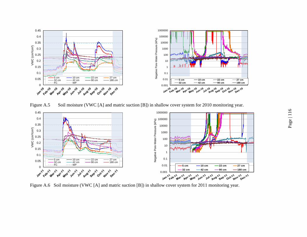
Pag
e | 1
16
Figure A.5 Soil moisture (VWC [A] and matric suction [B]) in shallow cover system for 2010 monitoring year.
Figure A.6 Soil moisture (VWC [A] and matric suction [B]) in shallow cover system for 2011 monitoring year.
0
0.05
0.1
0.15
0.2
0.25
0.3
0.35
0.4
0.45V
WC
(cm
³/cm
³)
5 cm 10 cm 22 cm 27 cm32 cm 42 cm 90 cm 180 cmFC WP
0.001
0.01
0.1
1
10
100
1000
10000
100000
1000000
Ne
ga
tive
Po
re-W
ate
r P
ressu
re (
kP
a)
5 cm 10 cm 22 cm 27 cm
32 cm 42 cm 90 cm 180 cm
0
0.05
0.1
0.15
0.2
0.25
0.3
0.35
0.4
0.45
VW
C (
cm
³/cm
³)
5 cm 10 cm 22 cm 27 cm32 cm 42 cm 90 cm 180 cmFC WP
0.001
0.01
0.1
1
10
100
1000
10000
100000
1000000
Ne
ga
tive
Po
re-W
ate
r P
ressu
re (
kP
a)
5 cm 10 cm 22 cm 27 cm
32 cm 42 cm 90 cm 180 cm
Pag
e | 1
17
Figure A.7 Soil moisture (VWC [A] and matric suction [B]) in deep cover system for 2006 monitoring year.
Figure A.8 Soil moisture (VWC [A] and matric suction [B]) in deep cover system for 2007 monitoring year.
0
0.05
0.1
0.15
0.2
0.25
0.3
0.35
0.4
0.45S
oil
VW
C (
cm
³/cm
³)
5 cm 10 cm 22 cm 27 cm 32 cm
42 cm 90 cm 180 cm FC WP
0.001
0.01
0.1
1
10
100
1000
10000
Ne
ga
tive
Po
re-W
ate
r P
ressu
re (
kP
a)
5 cm 22 cm 32 cm 47 cm
70 cm 90 cm 100 cm 180 cm
0
0.05
0.1
0.15
0.2
0.25
0.3
0.35
0.4
0.45
So
il V
WC
(cm
³/cm
³)
5 cm 10 cm 22 cm 27 cm 32 cm
42 cm 90 cm 180 cm FC WP
0.001
0.01
0.1
1
10
100
1000
10000
100000
1000000
Negative P
ore
-Wate
r P
ressure
(kP
a)
5 cm 22 cm 32 cm 47 cm
70 cm 90 cm 100 cm 180 cm

Pag
e | 1
18
Figure A.9 Soil moisture (VWC [A] and matric suction [B]) in deep cover system for 2008 monitoring year.
Figure A.10 Soil moisture (VWC [A] and matric suction [B]) in deep cover system for 2009 monitoring year.
0
0.05
0.1
0.15
0.2
0.25
0.3
0.35
0.4
0.45S
oil
VW
C (
cm
³/cm
³)
5 cm 10 cm 22 cm 27 cm 32 cm
42 cm 90 cm 180 cm FC WP
0.001
0.01
0.1
1
10
100
1000
10000
100000
1000000
Ne
ga
tive
Po
re-W
ate
r P
ressu
re (
kP
a)
5 cm 22 cm 32 cm 47 cm
70 cm 90 cm 100 cm 180 cm
0
0.05
0.1
0.15
0.2
0.25
0.3
0.35
0.4
0.45
So
il V
WC
(cm
³/cm
³)
5 cm 10 cm 22 cm 27 cm 32 cm
42 cm 90 cm 180 cm FC WP
0.001
0.01
0.1
1
10
100
1000
10000
100000
1000000
Ne
ga
tive
Po
re-W
ate
r P
ressu
re (
kP
a)
5 cm 22 cm 32 cm 47 cm70 cm 90 cm 100 cm 180 cm

Pag
e | 1
19
Figure A.11 Soil moisture (VWC [A] and matric suction [B]) in deep cover system for 2010 monitoring year.
Figure A.12 Soil moisture (VWC [A] and matric suction [B]) in deep cover system for 2011 monitoring year.
0
0.05
0.1
0.15
0.2
0.25
0.3
0.35
0.4
0.45S
oil
VW
C (
cm
³/cm
³)
5 cm 10 cm 22 cm 27 cm 32 cm
42 cm 90 cm 180 cm FC WP
0.001
0.01
0.1
1
10
100
1000
10000
100000
1000000
Negative P
ore
-Wate
r P
ressure
(kP
a)
5 cm 22 cm 32 cm 47 cm
70 cm 90 cm 100 cm 180 cm
0
0.05
0.1
0.15
0.2
0.25
0.3
0.35
0.4
0.45
So
il V
WC
(cm
³/cm
³)
5 cm 10 cm 22 cm 27 cm 32 cm
42 cm 90 cm 180 cm FC WP
0.001
0.01
0.1
1
10
100
1000
10000
100000
1000000
Negative P
ore
-Wate
r P
ressure
(kP
a)
5 cm 22 cm 32 cm 47 cm70 cm 90 cm 100 cm 180 cm

Page | 120
Appendix B
Electronic Supplements
Page | 121
Due to the volume of data collected while investigating this research topic, several data sets have
been compiled as supplements to this thesis. A complete list of data sets is as follows:
• Ambient Air Temperature 2005-2014
• Ambient PET 2005-2014
• Ambient PPT 2005-2014
• Berm Differential Pressures
• Deep Cover Differential Pressures
• Deep Cover Matric Suction
• Deep Cover Soil Temperatures
• Deep Cover VWC
• Deep Cover Water Balance – 2006
• Deep Cover Water Balance – 2007
• Deep Cover Water Balance – 2008
• Deep Cover Water Balance – 2009
• Deep Cover Water Balance – 2010
• Deep Cover Water Balance – 2011
• Deep Cover Water Balance – 2012
• Deep Cover Water Balance – 2013
• Deep Cover Water Balance – 2014
• Shallow Cover Differential Pressure
• Shallow Cover Matric Suction
• Shallow Cover Soil Temperature
• Shallow Cover VWC

Page | 122
• Shallow Cover Water Balance - 200
• Shallow Cover Water Balance – 2007
• Shallow Cover Water Balance – 2008
• Shallow Cover Water Balance – 2009
• Shallow Cover Water Balance – 2010
• Shallow Cover Water Balance – 2011
• Shallow Cover Water Balance – 2012
• Shallow Cover Water Balance – 2013
• Shallow Cover Water Balance - 2014