an evaluation of force reduction factor in seismic … · an evaluation of the force reduction...

An Evaluation of the Force Reduction Factor in the Force-Based Seismic Design

Gakuho Watanabe and Kazuhiko Kawashima Tokyo Institute of Technology, O-Okayama, Meguro, Tokyo, Japan, 152-8552

ABSTRACT This paper presents an analysis of the force reduction factors used in the force-based seismic design of structures. The force reduction factors are evaluated based on 70 free-field ground motions. Scattering of the force reduction factors depending on ground motions and the effect of damping rations assumed in linear and nonlinear responses are clarified. A new formulation of the force reduction factors is presented. KEY WORDS Seismic design, Forced-based design, Response modification factor, Force modification factor, Seismic response 1. INTRODUCTION In the force based seismic design, it is usual to estimate the demand from a linear response of a structure by dividing it by the force reduction factor. The force reduction factor or response modification factor, which is often called q-factor or R-factor, has an important role in the estimation of design force of a structure. An early study by Newmark and Hall (1973) revealed the fact that the equal displacement assumption and the equal energy assumption provide a good estimation of the force reduction factors at long and short periods, respectively. This affected an important effect to seismic design criteria worldwide.

Various researches such as Nassar and Krawinkler (1991) and Miranda and Bertero (1994) have been conducted on the force reduction factors. In particular, Miranda and Bertero provided a detailed review on the force reduction factors.

However, in spite of the importance in seismic design, less attention has been paid to large scattering of the force reduction factors depending on ground motions. Since the scattering is so large, only the mean values of the force reduction factor is not sufficient to evaluate a force reduction factor for design. Assumption of damping ratio for evaluating the linear and nonlinear responses is another important point. Although it has been general to assume the same damping ratio for the linear and nonlinear responses, it depends on how the force reduction factors are used.

This paper present an analysis on the force reduction factors based on 70 free-field ground motions. The scattering of the force reduction factors depending on ground motions and the effect of assumption of damping ratios in linear and nonlinear responses are clarified. 2. DEFINITION OF FORCE REDUCTION

FACTOR If one idealizes a structure in terms of a single-degree-of-freedom (SDOF) oscillator with an elastic perfect plastic bilinear hysteretic behavior as shown in Fig. 1, the force reduction

factor µR may be defined as

),,(

),(),,,(

NLTNL

Y

ELEL

RNLELT

TF

TFTR

ξµ

ξξξµµ = (1)

in which T : natural period, ELRF and NL

YF : maximum restoring force in an oscillator with a linear and a bilinear hysteresis, respectively, Tµ : target ductility factor, and ELξ and NLξ : damping ratio assumed in the evaluation of linear and bilinear responses, respectively. The natural period T may be evaluated based on the cracked stiffness of columns. Representing yu the yield displacement where the stiffness changes from the cracked stiffness to the post-yield stiffness, a target ductility factor Tµ may be defined based on the yielding displacement yu as

y

TT u

umax=µ (2)

in which Tumax is a target maximum displacement of an oscillator. The post-yield stiffness is assumed to be 0 in the present study.

Since the damping controls structural response, it has to be clarified carefully. A structure under a strong excitation generally exhibits strong hysteretic behavior, and this results in an energy dissipation in a structure. For example, the flexural inelastic deformation of columns contributes to energy dissipation in a bridge. Hence, the evaluation of damping ratio depends on the idealization of such an energy dissipation.

If one idealizes the energy dissipation in nonlinear structural components by incorporating nonlinear elements that represent the hysteretic behavior, the energy dissipation in the nonlinear structural components is automatically included in the analysis. On the other hand, if one idealizes the nonlinear structural components by elastic linear elements, the energy dissipation in the nonlinear structural components has to be included in the analysis by other means. The equivalent viscous damping ratio hξ is generally used for such a purpose as

WW

h∆⋅=

πξ

41 (3)

in which W∆ and W represent an energy dissipation in a hysteretic excursion and the elastic energy, respectively. For example, in an oscillator with an elastic perfect-plastic bilinear hysteresis, the equivalent damping ratio hξ is

µµ

πξ 12 −=h (4)

Fig. 2 shows the equivalent damping ratio by Eq. (4). It is generally very large such as 0.4 at the target ductility factor of 3-5.

In addition to such hysteretic energy dissipation, there must be some other sources of energy dissipation (for example, Kawashima, Unjoh, Tsunomoto 1993). The radiation of energy from a foundation to surround ground contributes to energy dissipation. Structural damping such as friction at connections may be important in many structures (for example, Kawashima and Unjoh 1989). Viscous damping due to friction with air is generally predominant in a structure with a long natural period. It is general to idealize those sources of energy dissipation in terms of the equivalent viscous damping.

If one considers a structure in which the flexural hysteretic energy dissipation is predominant with other sources of energy dissipation being a secondary importance, the total damping ratio eqξ of a SDOF oscillator

δδNLδELδY

F

FEL

FNL

O

Fig. 1 Definition of Force reduction Factor

may be provided as othheq ξξξ += (5)

in which hξ is the damping ratio that accounts the hysteretic energy dissipation by Eq. (3), and

othξ is the damping ratio that accounts the energy dissipation other than the hysteretic energy dissipation.

In the evaluation of the force reduction factor µR based on Eq. (1), how damping ratios are

assumed in the evaluation of the linear and the nonlinear responses is important. If one assumes the damping ratios as

eqEL ξξ = and othNL ξξ = (6) the energy dissipation is essentially the same between the linear and the nonlinear responses. Hence, the force reduction factor by Eq. (1) represents the difference of restoring force between the linear and nonlinear responses. Thus, Eq. (1) reflects the effect of nonlinear response of an oscillator.

On the other hand, if one assumes the damping ratios as

eqNLEL ξξξ == (7) or,

othNLEL ξξξ == (8) the force reduction factor by Eq. (1) includes the effect of different energy dissipation between the linear and nonlinear responses, in addition to the effect of nonlinear response. By assuming Eq. (7) in the evaluation of nonlinear response, the hysteretic energy dissipation in the nonlinear

structural components is counted by the equivalent viscous damping in addition to the inelastic excursion in the nonlinear elements. As a consequence, the hysteretic energy dissipation in the nonlinear structural components is counted twice in the evaluation of nonlinear response. On the other hand, if one assumes Eq. (8), the hysteretic energy dissipation is not taken into account in the evaluation of linear response. It should be noted here that which is appropriate among Eqs. (6), (7) and (8) depends on how the force reduction factor is used. Based on the original definition inherent to the force reduction factor, it seems that Eq. (6) is the most appropriate. Eq. (8) generally provides conservative estimation for the force reduction factors. If 0≈othξ , the difference of the force reduction factors among Eqs. (6), (7) and (8) is limited. It should be noted that hξ , othξ and eqξ depend on the type of a structure, mode shape, hysteresis and the target ductility factor.

Although the equivalent damping ratio hξ is very high as shown in Fig. 2, it is not general to assume such a high damping ratio in seismic design of a bridge structure. It is because a bridge structure is generally more complex than a SDOF oscillator, and this makes the relative contribution of the hysteretic energy dissipation of columns less significant. Since it is general practice in a standard bridge structure to assume about 0.05 for the damping ratio including hysteretic energy dissipation of columns, eqξ is assumed to be 0.05 in the present study based on Eq. (6). Hence, it is assumed here that hξ and othξ is 0.03 and 0.02, respectively.

Using those damping ratios, the force reduction factors are evaluated in this study based on Eq. (6). However, an analysis assuming Eqs. (7) and (8) is also conducted for comparison with the previous studies.

0

0.1

0.2

0.3

0.4

0.5

0.6

0 2 4 6 8

Equi

vale

nt D

ampi

ng

Rat

io ξ

Ductility Factor

h

Fig.2 Equivalent Damping Ratio hξ by Eq. (4)

3. REVIEW OF THE PAST INVESTIGATIONS

An early study for the force reduction factor was conducted by Newmark and Hall (Newmark and Hall 1973). They used 10 ground motions recorded in the 1940 Imperial Valley Earthquake. They assumed ELξ = NLξ =0.05, and proposed a force reduction factor as

( )

≤≤⋅⋅⋅⋅⋅⋅⋅⋅⋅⋅⋅⋅⋅⋅⋅⋅⋅⋅⋅⋅⋅⋅⋅≤≤′⋅⋅⋅⋅⋅⋅⋅⋅⋅⋅⋅⋅⋅⋅⋅⋅⋅

′≤≤⋅⋅⋅⋅⋅⋅⋅⋅⋅⋅−

≤≤⋅⋅⋅⋅⋅⋅⋅⋅⋅

−

≤≤⋅⋅⋅⋅⋅⋅⋅⋅⋅⋅

=

−

)( )( /

)4/( 12

)4/10/(

4

12

)10/0( 1

21

111

11

11

12/1log513.2

1

1

TTTTTTTT

TTT

TTTTT

TT

R

µµ

µ

µµ

µ

(9) where,

AV

Tea

evφφ

π21 =

12

11−

=′µµTT (10)

VD

Tev

edφφ

π21 =

in which, A , V and D represent peak ground acceleration, velocity and displacement, respectively, and eaφ , evφ and edφ represent the amplification for acceleration, velocity and displacement, respectively.

Nassar and Krawinkler proposed a force reduction factor, assuming ELξ = NLξ =0.05, based on an analysis for 15 ground motions as (Nassar and Krawinkler 1991)

{ } ccR /11)1( +−= µµ (11) where

Tb

TTTc ++

= α

αα

1),( (12)

in which α represents a ratio of the post-yield

stiffness to the initial elastic stiffness, and a and b are coefficients depending on α . Nassar and Krawinkler precisely analyzed the effect of stiffness deterioration, and provided the coefficients a and b depending on α .

Miranda and Bertero proposed a force reduction factor, assuming ELξ = NLξ =0.05, based on an analysis for 124 ground motions as (Miranda and Bertero 1994)

11),(

1 >+Φ

−=gTT

R µµ (13)

where,

⋅⋅⋅⋅⋅⋅⋅⋅⋅⋅⋅⋅⋅⋅⋅⋅⋅

−−−+

⋅⋅⋅⋅⋅⋅⋅⋅⋅⋅⋅⋅⋅⋅⋅⋅⋅

−−−

−+

⋅⋅⋅⋅⋅⋅⋅⋅⋅⋅⋅⋅⋅⋅⋅⋅⋅

−−−

−+

=Φ

(soft)

41ln3exp

43

31

(alluvium)

51ln2exp

52

1211

(rock)

53ln

23exp

21

1011

2

2

2

g

gg

TT

TT

TT

TTTT

TTTT

µ

µ

(14) in which gT represents a most predominant period.

It has been known that the equal energy assumption provides a good estimation for the force reduction factor at short periods while the equal displacement assumption at long periods. The force reduction factor provided by the equal energy and the equal displacement assumptions are given as

12 −= µµR (equal energy) (15) µµ =R (equal displacement) (16)

Application of Eqs. (15) and (16) and a comparison of the present study to the previous models will be described later.

4. FORCE REDUCTION FACTOR FOR BILINEAR OSCILLATORS

Force reduction factors were evaluated for target ductility factor Tµ of 2, 4, 6 and 8 assuming an elastic perfect-plastic bilinear hysteresis. Damping ratio in the linear and nonlinear analyses is assumed as ELξ =0.05 and NLξ =0.02 based on Eq. (6). Seventy free field ground accelerations by 64 shallow earthquakes with depth less that 60 km were used for analysis. They are classified into three soil conditions depending on the fundamental natural period of subsurface ground

gT ; stiff ( 2.0<gT s), moderate ( 6.02.0 <≤ gT s) and soft ( ≥gT 0.6 s) (Japan Road Association 2002). Number of records in the stiff, moderate and soft categories is 16, 39 and 15, respectively. Distribution of peak ground accelerations on the earthquake magnitudes and epicentral distances is shown in Fig. 3. The peak accelerations are in the range of 0.1-8m/s2, and the epicentral distances are in the range of 10-500 km.

Fig. 4 shows the force reduction factors for the 70 ground motions. Only the results for Tµ =4 and 6 are presented here since the results for other target ductility factors show the similar characteristics. It is seen in Fig. 4 that scattering of the force reduction factors depending on ground motions is significant. For example at natural period of 1 second, the force reduction factors varies from 1.9 to 10.3 depending on ground motions for Tµ =4 at the moderate soil sites. It is apparent that such a large scattering of the force reduction factors result in a large change of sizing of a structure in seismic design. Obviously smaller force reduction factors should be assumed in design to provide conservative design. It is observed in Fig. 4 that the dependence of force reduction factors on the soil condition is less significant. This will be discussed later.

Since the scattering of the force reduction

factors depending on ground motions is so large that the means +/- one standard deviations of the force reduction factors were obtained for each target ductility factor, natural period and soil condition. Fig. 5 shows the mean values and the mean values +/- one standard deviations of the force reduction factors presented in Fig. 4. The force reduction factors predicted by Eqs. (15) and (16) based on the equal displacement and the equal energy assumptions are also presented here for comparison. The mean values of force reduction factors increase as the natural periods increase, and then they approach to Tµ at long period. It has been pointed out in the previous researches that the Eq. (15) provides a good estimation to the force reduction factor. However, it is noted that Eq. (15) provides a good estimation to the mean values, but it considerably underestimates the force reduction factors corresponding to the mean values minus one standard deviations. On the other hand, Eq. (16)

0.1

1

10

10 100 1000Peak

Acc

eler

atio

n (m

/sec2 )

Epicentral Distance (km)

Stiff (Type-I)Moderate (Type-II)Soft (Type-IIII)

(a) Soil Condition

0.1

1

10

10 100 1000Peak

Acc

eler

atio

n (m

/sec2 )

Epicentral Distance (km)

6.5 - 7.07.0 - 7.57.5 - 8.0

(b) Earthquake Magnitude

Fig. 3 Classification of Ground Accelerations inTerms of Soil Conditions and EarthquakeMagnitudes

provides better estimation to the mean values minus one standard deviations. Taking account of the force reduction factors having considerable

scattering depending on ground motions, it seems reasonable to consider a certain redundancy in the estimation of the force reduction factor in design.

0

4

8

12

16

0 1 2 3 4Natural Period (s)

Rµ

fact

or

0

4

8

12

16

20

24


Rµ

fact

or

(a) Stiff (Type-I) (a) Stiff (Type-I)

0

4

8

12

16


Rµ

fact

or

0

4

8

12

16

20

24


Rµ

fact

or

(b) Moderate (Type-II) (b) Moderate (Type-II)

0

4

8

12

16


Rµ

fact

or

0

4

8

12

16

20

24


Rµ

fact

or

(c) Soft (Type-III) (c) Soft (Type-III)

(1) Tµ =4 (2) Tµ =6 Fig. 4 Force Reduction Factors

Based on such a consideration, it is more conservative to assume Eq. (16) instead of Eq. (15) for a design purpose.

Fig. 6 shows the dependence of the standard deviations of force reduction factors )( µσ R on the natural periods T and the soil condition. Similar to the mean values, the standard deviations )( µσ R increase as the natural periods increase, and decrease after taking peak values at natural period of 1-2 second. Fig. 7 shows the dependence of the standard deviations )( µσ R on the target ductility factors Tµ . The standard

deviations )( µσ R increase as the target ductility factors increase. The relation may be approximated by a least square fit as

⋅+−⋅+−⋅+−

=(soft) 409.0354.0

(moderate) 0.3780.292(stiff) 379.0328.0

)( T

T

T

Rµµµ

σ µ (17)

As the soil condition dependence of )( µσ R is less significant as shown in Fig. 7, Eq. (17) may be approximated as

TR µσ µ ⋅+−≈ 4.03.0)( (18)

Average + 1σ

Average - 1σAverage

Rµ = 2µ-1Rµ = µ

0

4

8

12


Rµ

fact

or

0

4

8

12


Rµ

fact

or


0

4

8

12


Rµ

fact

or

0

4

8

12


Rµ

fact

or


0

4

8

12


Rµ

fact

or

0

4

8

12


Rµ

fact

or

(c) Soft (Type-III) (c) Soft (Type-III) (1) Tµ =4 (2) Tµ =6

Fig. 5 Mean and Mean +/- One Standard Deviation of the Force Reduction Factors for 70 Ground Motions

0 1 2 3 4 5

Rµ f

acto

r

Natural Period (s)

µ

1 a

(µ−1)

1/b

Pc Q

0

Fig. 8 Idealization of Force Reduction Factors

5. FORMULATION OF FORCE REDUCTION FACTORS

To idealize the mean values of the force reduction factors in Fig. 5, they are represented as

1)()1( +Ψ⋅−= TR µµ (19)

where,

1)( )( +−⋅=Ψ −⋅ aTbeaTcT (20)

in which a , b and c are parameters to be determined.

Since µµ =R at aT = in Eq. (20), the parameter a represents the period where µR is equal to µ (Point P) as shown in Fig. 8. Because the gradient of µR is

)()(1)1( aTbe

aTbcdT

dR−−−⋅−= µµ (21)

it is )1( −⋅ µc at Point P. Consequently, the parameter c represents the gradient at Point c divided by 1−µ . Representing Q as the point where µR takes the peak value, b/1 represents the period between Points P and Q.

Based on the definition, the following condition has to be satisfied in µR

0lim0

=→

µRT

(22)

Hence, the coefficient c can be eliminated as abaec /1= (23)

Substitution of Eq. (23) makes Eq. (20) as

1)( +−=Ψ bTaeaTT (24)

It is noted that Eq. (19) automatically satisfies the following condition

µµ =∞→R

T lim (25)

0

2

4

6

8

0 1 2 3 4

Stiff (Type-I)Moderate (Type-II)Soft (Type-III)

Natural Period (s)

σ ( R

µ )

(a) Tµ =4

0

2

4

6

8


σ ( R

µ )

(b) Tµ =6

Fig. 6 Natural Period Dependence of StandardDeviations of the Force ReductionFactors

0

2

4

6

8

10

0 2 4 6 8 10


Target Ductility µT

σ (R

µ)

Fig. 7 Target Ductility Factor Dependence ofthe Standard Deviations of Forcereduction Factors

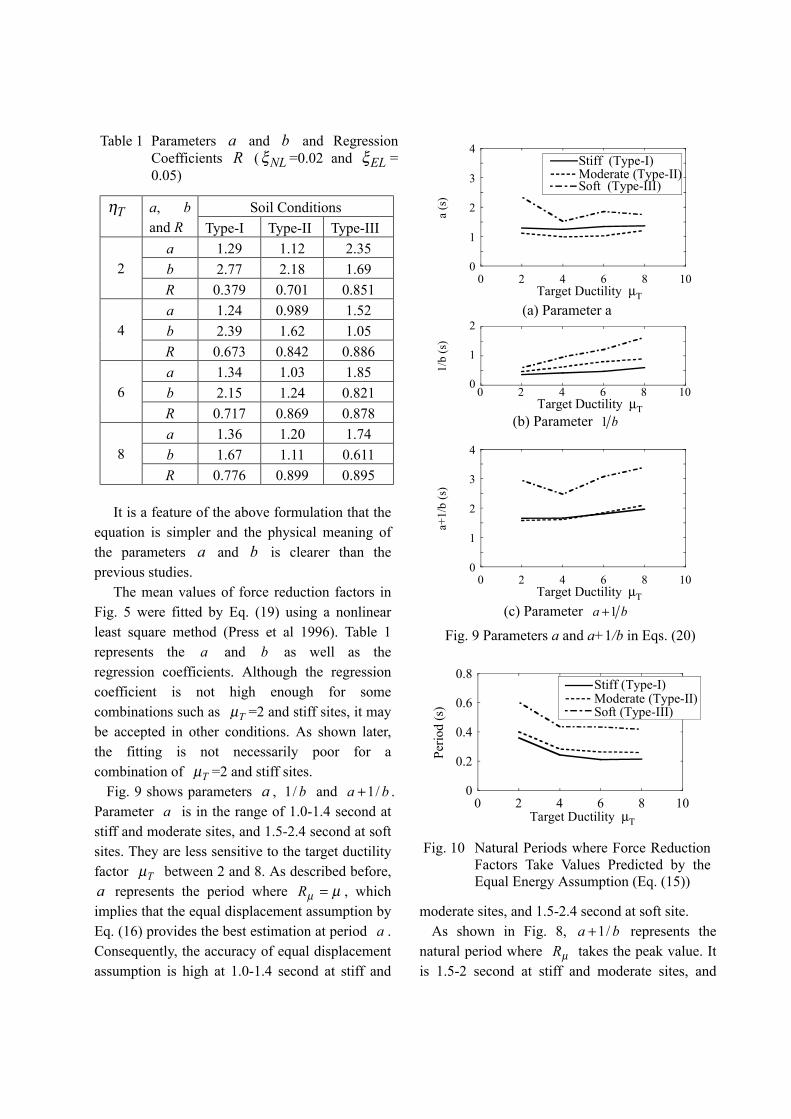
It is a feature of the above formulation that the equation is simpler and the physical meaning of the parameters a and b is clearer than the previous studies.

The mean values of force reduction factors in Fig. 5 were fitted by Eq. (19) using a nonlinear least square method (Press et al 1996). Table 1 represents the a and b as well as the regression coefficients. Although the regression coefficient is not high enough for some combinations such as Tµ =2 and stiff sites, it may be accepted in other conditions. As shown later, the fitting is not necessarily poor for a combination of Tµ =2 and stiff sites.

Fig. 9 shows parameters a , b/1 and ba /1+ . Parameter a is in the range of 1.0-1.4 second at stiff and moderate sites, and 1.5-2.4 second at soft sites. They are less sensitive to the target ductility factor Tµ between 2 and 8. As described before, a represents the period where µµ =R , which implies that the equal displacement assumption by Eq. (16) provides the best estimation at period a . Consequently, the accuracy of equal displacement assumption is high at 1.0-1.4 second at stiff and

moderate sites, and 1.5-2.4 second at soft site. As shown in Fig. 8, ba /1+ represents the

natural period where µR takes the peak value. It is 1.5-2 second at stiff and moderate sites, and

0

1

2

3

4

0 2 4 6 8 10

a (s

)

Target Ductility µΤ


(a) Parameter a

0

1

2

0 2 4 6 8 10

1/b

(s)

Target Ductility µΤ (b) Parameter b1

0

1

2

3

4

0 2 4 6 8 10

a+1/

b (s

)

Target Ductility µΤ (c) Parameter ba 1+

Fig. 9 Parameters a and a+1/b in Eqs. (20)

Table 1 Parameters a and b and Regression Coefficients R ( NLξ =0.02 and ELξ = 0.05)

Soil Conditions Tη a, b and R Type-I Type-II Type-III

a 1.29 1.12 2.35 b 2.77 2.18 1.69

2

R 0.379 0.701 0.851 a 1.24 0.989 1.52 b 2.39 1.62 1.05

4

R 0.673 0.842 0.886 a 1.34 1.03 1.85 b 2.15 1.24 0.821

6

R 0.717 0.869 0.878 a 1.36 1.20 1.74 b 1.67 1.11 0.611

8

R 0.776 0.899 0.895

0

0.2

0.4

0.6

0.8

0 2 4 6 8 10

Perio

d (s

)

Target Ductility µΤ


Fig. 10 Natural Periods where Force ReductionFactors Take Values Predicted by theEqual Energy Assumption (Eq. (15))

2.5-3.5 second at soft site. It slightly increases as target ductility Tµ increases.

The natural periods where µR take the values predicted by Eq. (15) based on the equal energy assumption are obtained as shown in Fig. 10. They are in the range of 0.2-0.36 second, 0.26-0.4 second and 0.4-0.6 second at stiff, moderate and

soft sites, respectively. They are much shorter than the natural periods where the equal displacement assumption provides the best approximation.

Fig. 11 compares the mean force reduction factors presented in Fig. 5 to the values predicted by Eq. (19). Although some discrepancies are observed at larger target ductility factors, Eq. (19)

µT = 2µT = 4µT = 6µT = 8

Empirical Model Mean

0

4

8

12

16


Rµ

fact

or

(a) Stiff (Type-I)

0

4

8

12

16


Rµ

fact

or

(b) Moderate (Type-II)

0

4

8

12

16


Rµ

fact

or

(c) Soft (Type-III)

Fig. 11 Application of Eq. (19) to the MeanForce Reduction Factors Presented inFig. 5

0

4

8

12


Rµ f

acto

r Stiff (Type-I)Moderate (Type-II)Soft (Type-III)

(a) Tµ =2

0

4

8

12


Rµ f

acto

r

(b) Tµ =4

0

4

8

12


Rµ f

acto

r

(c) Tµ =6

0

4

8

12


Rµ f

acto

r

(d) Tµ =8

Fig. 12 Effect of Soil Condition on the ForceReduction Factors Predicted by Eq.(19)

provides a good estimation for the mean force reduction factors.

Fig. 12 shows the effect of soil condition on the mean force reduction factors estimated by Eq. (19). The effect of soil condition is less significant on the force reduction factors, in particular at small target ductility factors.

As shown in Fig. 4, scattering of the force reduction factors around the mean values is extensive. Hence, the force reduction factors corresponding to the mean values m substituted by a standard deviation )( µσ R are evaluated as shown in Fig. 13. The mean and the standard deviation of force reduction factors were evaluated by by Eq. (19) and Eq. (18), respectively, in this estimation. They are of course

close to the force reduction factors of the mean minus one standard deviation directly computed from the 70 ground motions (refer to Fig. 5). The force reduction factors predicted by Eq. (15) based on the equal energy assumption are presented here for comparison. From Fig. 13, it is seen that at Tµ =4, the equal energy assumption provides a good estimation at natural periods longer than 0.5 second at stiff and moderate sites and 1.2 second at soft sites, while it provides underestimation at natural periods shorter than those values. On the other hand, at Tµ =8, the equal energy assumption provides a good estimation at 0.6 second at stiff and moderate sites and 1 second at soft sites. It underestimates and overestimates the force reduction factors

0

4

8

12


Rµ =3.87

Rµ =2.65

Rµ f

acto

r

µΤ = 8

µΤ = 4

(a) Stiff (Type-I)

0

4

8

12


Rµ =3.87

Rµ =2.65

Rµ f

acto

r

µΤ = 8

µΤ = 4

(b) Moderate (Type-II)

0

4

8

12


Rµ =3.87

Rµ =2.65

Rµ f

acto

r

µΤ = 8

µΤ = 4

(c) Soft (Type-III)

Fig.13 Force Reduction Factors Corresponding toMeans minus One Standard Deviations

Table 2 Parameters a and b ( NLξ = ELξ = 0.02)

Soil Conditions Tµ

a and b Type-I Type-II Type-III a 0.152 0.225 0.361 2 b 0.289 1.60 1.12 a 0.289 0.348 0.600 4 b 2.46 1.28 0.902 a 0.397 0.432 0.800 6 b 1.81 1.14 0.768 a 0.507 0.513 0.916 8 b 1.14 1.04 0.632

Table 3 Parameters a and b ( NLξ = ELξ = 0.05)

Soil Conditions Tµ

a and b Type-I Type-II Type-III a 0.226 0.344 0.521 2 b 4.14 1.94 1.34 a 0.778 0.572 0.976 4 b 3.50 1.35 0.994 a 0.981 0.725 1.23 6 b 2.93 1.15 0.757 a 1.23 0.807 1.28 8 b 2.57 0.983 0.569

corresponding to the mean minus one standard deviation at natural periods shorter and longer, respectively, than the above natural periods. 6. EFFECT OF DAMPING RATIOS In the preceding analysis, the force reduction factors were evaluated based on Eq. (1) assuming

ELξ =0.05 and NLξ =0.02. However in the past researches, damping ratios were usually assumed as ELξ = NLξ =0.05. Consequently, the same analysis presented in the preceding chapters was conducted by assuming ELξ = NLξ =0.05 based on Eq. (7) using the same ground motion data set.

For comparison, an analysis was also conducted assuming ELξ = NLξ =0.02 based on Eq. (8).

Tables 2 and 3 show the parameters a and b determined for a combination of ELξ = NLξ =0.02 and ELξ = NLξ =0.05, respectively. Fig. 14 compares a and ba /1+ thus determined. Also presented in Fig. 14 are a and ba /1+ used in the preceding chapter ( ELξ =0.05 and NLξ =0.02, refer to Fig. 9). It is seen in Fig. 14 that both a and ba /1+ at the same target ductility factors are the shortest for a combination of

ELξ = NLξ =0.02 and the longest for a combination of ELξ =0.05 and NLξ =0.02. Parameters a and ba /1+ for a combination of

ELξ = NLξ =0.05 are between the two cases.

ξNL = ξEL = 0.02ξNL = 0.02, ξEL = 0.05ξNL = ξEL = 0.5

0

1

2

3

0 2 4 6 8 10µΤTarget Ductility

a (s

)

01

23


a+1/

b (s

)


0

1

2

3


a (s

)

01

23


a+1/

b (s

)


0

1

2

3


a (s

)

01

23


a+1/

b (s

)

(c) Soft (Type-III) (c) Soft (Type-III) (1) Parameter a (2) Parameter a+1/b

Fig. 14 Dependence of Parameters a and a+1/b on the Assumption of Damping Ratios

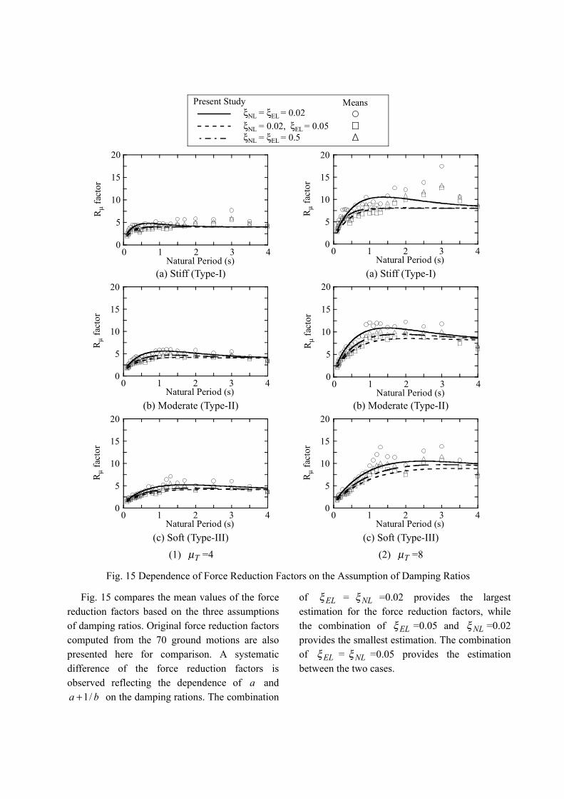
Fig. 15 compares the mean values of the force reduction factors based on the three assumptions of damping ratios. Original force reduction factors computed from the 70 ground motions are also presented here for comparison. A systematic difference of the force reduction factors is observed reflecting the dependence of a and

ba /1+ on the damping rations. The combination

of ELξ = NLξ =0.02 provides the largest estimation for the force reduction factors, while the combination of ELξ =0.05 and NLξ =0.02 provides the smallest estimation. The combination of ELξ = NLξ =0.05 provides the estimation between the two cases.

ξNL = ξEL = 0.02ξNL = 0.02, ξEL = 0.05ξNL = ξEL = 0.5

Present Study Means

0

5

10

15

20

0 1 2 3 4

Rµ f

acto

r

Natural Period (s)

0

5

10

15

20

0 1 2 3 4

Rµ f

acto

r

Natural Period (s) (a) Stiff (Type-I) (a) Stiff (Type-I)

0

5

10

15

20

0 1 2 3 4

Rµ f

acto

r

Natural Period (s)

0

5

10

15

20

0 1 2 3 4

Rµ f

acto

r

Natural Period (s) (b) Moderate (Type-II) (b) Moderate (Type-II)

0

5

10

15

20

0 1 2 3 4

Rµ f

acto

r

Natural Period (s)

0

5

10

15

20

0 1 2 3 4

Rµ f

acto

r

Natural Period (s) (c) Soft (Type-III) (c) Soft (Type-III) (1) Tµ =4 (2) Tµ =8

Fig. 15 Dependence of Force Reduction Factors on the Assumption of Damping Ratios

7. COMPARISON WITH THE PREVIOUS STUDIES Fig. 16 shows a comparison of the force reduction factor in the present study by Eq. (19) to Nassar and Krawinkler by Eq. (11) and Miranda and Bertero by Eq. (13). Since it is assumed in Eqs. (11) and (13) that ELξ = NLξ =0.05, the same

damping ratios are assumed in the present study for comparison. The original mean values of the force reduction factors computed from the 70 ground motions are also presented here for comparison. It is noted that definition of soil conditions is not the same among three researches. Hence they are classified into stiff, moderate and soft. In the Miranda and Bertero formulation, gT

Present StudyMeansMiranda et al.

Nassar et al.

0

4

8

12

16


Rµ

fact

or

0

4

8

12

16


Rµ f

acto

r


0

4

8

12

16


Rµ f

acto

r

0

4

8

12

16


Rµ f

acto

r


0

4

8

12

16


Rµ f

acto

r

0

4

8

12

16


Rµ f

acto

r

(c) Soft (Type-III) (c) Soft (Type-III) (1) Tµ =4 (2) Tµ =8

Fig. 16 Comparison with Previous Studies

was assumed 1.5 second at soft (alluvial) site in Eq. (14).

From Fig. 16, it is seen that the present study provides a quite similar result to the formulations by Miranda & Mertero and Nassar & Krawinkler if the same damping ratios are assumed in the evaluation of linear and nonlinear responses. 8. CONCLUSIONS An analysis was conducted for the force reduction factor based on response of SDOF oscillator using 70 free-field ground motions. Based on the analysis presented herein, the following conclusions may be deduced: 1) A new formulation as shown in Eqs. (19) and (24) was developed. The formulation is simpler than the past formulations. Parameters a and a +1/b express the natural period where µR is equal to µ and µR takes a peak value, respectively. 2) Difference of the damping ratios assumed in the evaluation of linear and nonlinear responses ( ELξ and NLξ ) provides a systematic difference in the force reduction factors. The combination of

ELξ = NLξ =0.02 provides the largest estimation for the force reduction factors, while the combination of ELξ =0.05 and NLξ =0.02 provides the smallest estimation. The combination of ELξ = NLξ =0.05 provides the estimation between the two cases. Hence, the damping ratios have to be carefully assumed keeping how the force reduction factors are used in mind. 3) Scattering of the force reduction factors depending on ground motions is significant. Although it has been pointed out that the equal displacement assumption by Eq. (15) provides a good estimation to the force reduction factors, it provides a good estimation only to the mean values; however, it considerably underestimates

the mean minus one standard deviation. On the other hand, the equal energy assumption by Eq. (16) provides a better estimation to the force reduction factors corresponding to the mean minus one standard deviation, although it provides too conservative estimation to the mean values. Taking account of the considerable scattering of the force reduction factors depending on ground motions, it is conservative to assume the equal energy assumption instead of the equal displacement assumption. 4) The response modification factors in the present study by Eqs. (19) and (24) provides quite close force reduction factors proposed by Nassar and Krawinkler, and Miranda and Betero, if the damping ratios are assumed as ELξ = NLξ =0.05. REFERENCES Japan Road association (2002), Part V Seismic

design, Design specifications of highway bridges,” Maruzen, Tokyo, Japan.

Kawashima, K, MacRae, G. A., Hoshikuma, J. and Nagaya, K. (1998). “Residual displacement response spectra,” Journal of Structural Engineering, 124(5), 513-530, ASCE

Kawashima, K. and Unjoh, S. (1989). “Damping characteristics of cable-stayed bridges associated with energy dissipation at movable support,” Structural Engineering and Earthquake Engineering, Proc. Japan Society of Civil Engineers, 404/I-11, 123-130.

Kawashima, K., Unjoh, S. and Tsunomoto, M. (1993). “Estimation of damping ratio of cable-stayed bridges for seismic design,” Journal of Structural Engineering, 119(4), 1015-1031, ASCE.

Miranda, E. and Bertero, V. (1994). “Evaluation of strength reduction factors for earthquake resistant design,” Earthquake Spectra, 10(2), 357-379.

Nassar, A. A. and Krawinkler, H. (1991). “Seismic demands for SDOF and MDOF systems,” Report No. 95, The John A. Blume Earthquake Engineering Center, Stanford University, California, USA.

Newmark, N. M. and Hall, W. J. (1973). “Seismic design criteria for nuclear reactor facilities,” Report No. 46, Building Practices for Disaster Mitigation, National Bureau of Standards, U.S. Department of Commerce, 209-236.

Press, W.H., Teukolsky, S.A., Vetterling, W.T. and

Flannery, B.P. (1996). “Numerical recipes in Fortran 77,” Second Edition, The Art of Scientific Computing, Cambridge University Press, 678-683.

Priestley, M. J. N., Seible, F. and Calvi, G. M. (1996). “Seismic design and retrofit of bridges,” John Wiley & Sons, New York, USA.

Takeda, T., Sozen, M. A. and Nielsen, N. N. (1970). “Reinforced concrete response to simulated earthquake,” Journal of Structural Engineering, 96(12), 2557-2573, ASCE

an evaluation of force reduction factor in seismic … · an evaluation of the force reduction...

Documents