an evaluation of the global patterns of atmospheric -...

EUR 24264 EN - 2010

An evaluation of the global patterns of atmospherictransport for regionalized chemical risk assessment

Alberto Pistocchi, Grazia Zulian, Paolo Isoardi

The mission of the JRC-IES is to provide scientific-technical support to the European Union’s policies for the protection and sustainable development of the European and global environment. European Commission Joint Research Centre Institute for Environment and Sustainability Contact information Address: Alberto Pistocchi, JRC, TP 460, Via Fermi 2749, 21027 Ispra (VA), Italy E-mail: [email protected] Tel.: 00 39 0332 785591 Fax: 00 39 0332 785601 http://ies.jrc.ec.europa.eu/ http://www.jrc.ec.europa.eu/ Legal Notice Neither the European Commission nor any person acting on behalf of the Commission is responsible for the use which might be made of this publication.

Europe Direct is a service to help you find answers to your questions about the European Union

Freephone number (*):

00 800 6 7 8 9 10 11

(*) Certain mobile telephone operators do not allow access to 00 800 numbers or these calls may be billed.

A great deal of additional information on the European Union is available on the Internet. It can be accessed through the Europa server http://europa.eu/ JRC 56210 EUR 24264 EN ISBN 978-92-79-15063-0 ISSN 1018-5593 doi:10.2788/65179 Luxembourg: Publications Office of the European Union © European Union, 2010 Reproduction is authorised provided the source is acknowledged Printed in Italy

3

Table of content

1. Introduction and purpose of the research ................................................................................ 4

2. Derivation of global patterns of atmospheric transport .......................................................... 5

2.1 Emission grids creation ............................................................................. 5 2.1.1 Data ....................................................................................................... 5 2.1.2 Methodology ......................................................................................... 6

2.2 Numerical simulations with the HySPLIT model ................................... 11 2.2.1 Data ..................................................................................................... 11 2.2.2 Methodology ....................................................................................... 11 2.2.3 Output processing ............................................................................... 19

3. Investigation of the relationship between concentration and distance from emission .......... 23

4. Implications for global scale comparative chemical risk assessment: an example about

the variability of impacts due to the location of the emission ...................................................... 49

5. Acknowledgements ............................................................................................................... 53

6. References ............................................................................................................................. 53

4

1. Introduction and purpose of the research In chemical risk assessment, often simple non spatial models are used (e.g. EC,

2003,2004). These models represent the area of interest as a box or continuous stirred tank reactor, where an average concentration is computed from emissions and local removal rates including advection, deposition and degradation of the chemical. This simple scheme has many advantages and is basically appropriate to depict first-level figures of atmospheric exposure to contaminants. However, it does not allow accounting for effects of an atmospheric emission, at locations other than the one of emission.

The standard alternative to a box model is an atmospheric transport model which solves the advection-dispersion equation, and can be in analytical (e.g. a Gaussian plume model) or numerical form (see e.g. Pistocchi, 2008, for a more thorough discussion). Analytical models can be only applied to situations where wind has a dominant direction that does not change significantly, which is the case only for local assessment (e.g. a few to a few tens of kilometers); when moving to broader scales, numerical models need to be used due to the complex wind fields occurring in the regional or even global atmosphere. Although routinely used for certain types of applications, complex numerical air transport models do not appear sufficiently practical for the standard lower tiers of chemical risk assessment, when one has to cope with generic emission scenarios and limited information and knowledge on the physico-chemical properties and environmental fate of contaminants. The same type of consideration holds for applications in such contexts as Life Cycle Impact Assessment (LCIA) of services or products, where evaluations are referred to more generic scenarios than required for the implementation of realistic numerical simulations.

Pistocchi and Galmarini, 2008, while evaluating the European source-receptor model ADEPT, found that patterns of atmospheric transport at the European scale, as represented by the mean annual concentration arising from a continuous emission spatially distributed in proportion to human population, could be well approximated by a function of the Euclidean distance from the source, and particularly by the inverse of distance raised to 4/3. In this report, we illustrate an investigation conducted to test whether this approximation can be used also for the global scale of atmospheric transport from local sources. Were it to hold, such an approximation would provide a method as quick and simple as box models, but capable to describe effects of an atmospheric emission not just at the location of emission, but also away in space.

In order to test the simple model of Pistocchi and Galmarini, 2008, we followed the steps described more in detail in the paragraphs hereafter:

1) build a plausible spatial distribution of emissions of chemicals related to human use, and assumed to be continuous in time; the proxy adopted for human activity intensity on a global scale was the intensity of lights at night;

2) cluster emissions in homogeneous emission zones each of which is investigated independently, as it is not likely that a chemical is used globally in proportion to population density only;

3) run a numerical model (the well known HySPLIT, quickly described below) to derive consistent spatial distributions of average annual concentrations arising from each of the above emission clusters;

4) investigate the relationship between annual average concentrations from a continuous emission, and the Euclidean distance from the emissions.

5 When tackling the tasks in practical terms, it was apparent that running a one-year-long global simulation of continuous emissions for each homogeneous emission zone using HySPLIT would simply take too long for practical purposes. Therefore, it was decided to run a calculation for the months of January and July, and to approximate the annual average concentration as the average of the two. Tests on the reaching of reasonably steady spatial distribution of mass from emissions support the idea that this approximation is reasonable for practical applications. Simulations were run for a generic, conservative contaminant and depict the effect of atmospheric dilution and transport, through advection and dispersion. The global-scale maps of generic pollutant concentrations can be used as inputs for further studies (e.g. source-receptor relationship, time of travel) which are not further discussed in the present report.

2. Derivation of global patterns of atmospheric transport

This part of the document describes firstly the procedure to create the global emission grid files to be used as input into the HySPLIT (Hybrid Single-Particle Lagrangian Integrated Trajectory) model; then the setup of the modeling software and the processing of the outputs.

2.1 Emission grids creation Polluted areas on the globe are assumed to be proportionally related to nighttime

stable lights emissions, which are generated from human settlements as urban and industrial areas.

The output grids are an estimation of emission points from the most populated and developed area of the world.

2.1.1 Data “The Defense Meteorological Satellite Program (DMSP) Operational Linescan

System (OLS) has a unique low-light imaging capability developed for the detection of clouds using moonlight. In addition to moonlit clouds, the OLS also detects lights from human settlements, fires, gas flares, heavily lit fishing boats, lightning and the aurora. By analyzing the location, frequency, and appearance of lights observed in an image time series, it is possible to distinguish four primary types of lights present at the earth's surface: human settlements, fires, gas flares, and fishing boats. We have produced a global map of the four types of light sources as observed during a 6-month period in 1994 - 1995” (Elvidge et al., 2001).

World stable lights percent frequency files (cities and flares combined) were retrieved from the Internet at http://www.ngdc.noaa.gov/dmsp/download_Night_time_lights_94-95.html

The lower resolution file (filename_low_res.tif) was used, that contains byte images in a geographic projection with size: 21600 x 10800 cells, grid spacing of 1 Arc second, upper left pixel (90 North, -180 East), in TIFF format (Figure 1).

6

Figure 1. DMSP World Stable lights.

The data were aggregated on a global 2.5°x2.5° grid, where 10368 (144x72) centroids were identified from global fishnet with 2.5 cell size, in geographic coordinate system WGS84, Shapefile format; for further clustering, also a map of World Countries as of 2002 in geographic coordinate system WGS84, Shapefile format was also used as retrieved from the internet at: http://openmap.bbn.com/data/shape/cntry02.tar.gz.

2.1.2 Methodology 1) Re-sampling of DMSP World Stable Lights dataset to 2.5°x2.5° cell size (using the

Block statistics tool from Spatial Analyst).

Figure 2. DMSP World Stable lights re-sampled.

2) Selection of points from the 2.5°x2.5° grid which are completely within the

country polygons (Select by Location).

3) Extract light intensity values from the re-sampled lights dataset to 2) (Extract Values to Points tool).

4) Extract country names to 3) (Spatial Join tool).

7

5) Select points with light intensity values > 0.5 and export data as new shapefile (Figure 3).

Figure 3. Emission points.

6) Aggregation of involved countries into 20 clusters (Figure 4):

1. Australia + New Zealand. 2. Canada + Alaska. 3. Central America: Belize, Dominican Republic, El Salvador, Guadeloupe, Mexico,

Nicaragua, Panama. 4. Northern Africa: Algeria, Egypt, Libya, Morocco, Sudan, Tunisia. 5. Western Africa: Cote d'Ivory, Equatorial Guinea, Ghana, Nigeria, Togo, Angola, Congo. 6. Southern Africa: Botswana, Congo DRC, Lesotho, South Africa, Swaziland, Zambia,

Zimbabwe, Kenya, Tanzania. 7. Central Asia: Kazakhstan, Kyrgyzstan, Tajikistan, Turkmenistan, Uzbekistan. 8. Eastern Asia: Japan, North Korea, South Korea. 9. North-East Asia: China, Mongolia, Taiwan. 10. South-East Asia: Indonesia, Laos, Malaysia, Myanmar, Philippines, Thailand, Vietnam. 11. Southern Asia: Afghanistan, Bangladesh, India, Pakistan. 12. Europe: Belgium, Bosnia & Herzegovina, Bulgaria, Croatia, Czech Republic, Denmark,

Estonia, Finland, France, Germany, Greece, Hungary, Ireland, Italy, Latvia, Lithuania, Macedonia, Norway, Poland, Portugal, Romania, Slovakia, Spain, Sweden, Switzerland, United Kingdom, Yugoslavia.

13. Eastern Europe: Azerbaijan, Belarus, Georgia, Moldova, Russia, Ukraine. 14. Middle East: Iran, Iraq, Jordan, Oman, Saudi Arabia, Syria, United Arab Emirates, Yemen. 15. Turkey. 16. Eastern South-America: Brazil, Paraguay. 17. Northern South-America: Colombia, Ecuador, Venezuela. 18. Southern South-America: Argentina, Chile, Uruguay. 19. United States. 20. Western South-America: Bolivia, Peru.

8

Figure 4. Clusters of emission points.

7) Normalization of light intensity values per country group, so that the sum of all

points within each group equals to 1 (performed in Excel)

8) Join table 7) with 6) and export as new shapefile. The final dataset looks as shown in Figure 5.

OBJECTID POINT_X POINT_Y I J AREA_NAME NORM

_VAL 4867 106.25 -6.25 115 34 South-East Asia 0.438286303

… … … … … … …Figure 5 – example of the final data set

9) generation of 20 emission grid files (one per country group) in a format suitable to be used as input into HySPLIT modeling software, using a taylor-made python script “HySPLIT_export.py” as listed below. '''--------------------------------------------------------------------------------

---- Tool Name: HySPLIT_export Source Name: HySPLIT_export.py Version: ArcGIS 9.2 Author: Paolo Isoardi Email: [email protected] Date: 18/08/2008 Argumuments: Point feature layer Output folder Description: create gridded emissions files in plain text format to be used as

input into HySPLIT software (http://www.arl.noaa.gov/ready/HySPLIT4.html) Note: Requires a point feature layer with the following attributes: POINT_X, POINT_Y, GROUP_NAME, POLLUTANT_VALUE, (I), (J) The format of the emission data file: |->Loop through the number of i,j grid point | | Record #1 (2I4) I,J grid point index of emission cell | (2F10.4) Southwest cell corner (longitude & Latitude) | | |->Loop through the number of pollutant species

9 | | | | Record #2 (12E10.3) pollutant #1 for GMT hours 1-12 | | Record #3 (12E10.3) pollutant #1 for GMT hours 13-24 I.E.: 78.0 33.0 13.75 -8.75 0.14954 0.14954 0.14954 0.14954 0.14954 0.14954

0.14954 0.14954 0.14954 0.14954 0.14954 0.14954 0.14954 0.14954 0.14954 0.14954 0.14954 0.14954

0.14954 0.14954 0.14954 0.14954 0.14954 0.14954 -----------------------------------------------------------------------------------

-''' try: # import system modules and create the Geoprocessor object try: # the v9.2 way import arcgisscripting, os, sys, string gp = arcgisscripting.create() except: try: # the v9.0 & v9.1 way import win32com.client, string, sys, os gp = win32com.client.Dispatch(

"esriGeoprocessing.GpDispatch.1" ) except: print "ERROR: can't create the gp object!!!" # start feedback gp.AddMessage( "\n==========[ START ]==========\n" ) # check out the highest grade license available if gp.CheckProduct( "ArcInfo" ) == "Available": gp.SetProduct( "ArcInfo" ) elif gp.CheckProduct( "ArcEditor" ) == "Available": gp.SetProduct( "ArcEditor" ) elif gp.CheckProduct( "ArcView" ) == "Available": gp.SetProduct( "ArcView" ) else: raise Exception, "ArcGIS licenses error"; gp.AddMessage( gp.ProductInfo()+" license selected" ) # enable overwrite gp.overwriteoutput = 1 # get input arguments inputPointLayer = gp.GetParameterAsText(0) outputFolder = gp.GetParameterAsText(1) inputLonField = gp.GetParameterAsText(2) inputLatField = gp.GetParameterAsText(3) inputAreaField = gp.GetParameterAsText(4) inputEmissionField = gp.GetParameterAsText(5) inputIField = gp.GetParameterAsText(6) inputJField = gp.GetParameterAsText(7) # check layer geometry type dsc = gp.Describe( inputPointLayer ) if dsc.ShapeType != "Point": raise Exception, "Input layer must be of Point type" # check outputFolder for white spaces if outputFolder.find(" ") != -1: raise Exception, "Output folder must not contain white spaces in its

name" # set work space and scratch space gp.Workspace = outputFolder gp.scratchWorkspace = outputFolder # counter n = 1

10 N = gp.GetCount_management( inputPointLayer ) n_points = 0 # loop through the input points to create concentration rasters rows = gp.SearchCursor( inputPointLayer, "", "", "", inputAreaField+" A" ) rows.reset() row = rows.next() while row: # Create the Text File to write data to (one file per group) if n == 1: outputFileName = str(row.getvalue(inputAreaField)) + ".txt" outputFile = open( outputFolder + "/" + outputFileName, "w" ) gp.AddMessage( "writing to: " + outputFileName ) else: if not outputFileName == str(row.getvalue(inputAreaField)) +

".txt" : gp.AddMessage( " (" + str(n_points) + "

points)" ) n_points = 0 outputFile.close() outputFileName = str(row.getvalue(inputAreaField)) +

".txt" outputFile = open( outputFolder + "/" +

outputFileName, "w" ) gp.AddMessage( "writing to: " + outputFileName ) if n == N: gp.AddMessage( " (" + str(n_points+1) + "

points)" ) # check if I and J fields exist, oterwhise set I=0 and J=0 if not inputIField: inputIFieldValue = 0 else: inputIFieldValue = row.getvalue(inputIField) if not inputJField: inputJFieldValue = 0 else: inputJFieldValue = row.getvalue(inputJField) # write data to file outputFile.write(" " + str(inputIFieldValue) + " " +

str(inputJFieldValue) + " " + str(row.getvalue(inputLonField)) + " " + str(row.getvalue(inputLatField)) + "\n")

outputFile.write(" " + str(row.getvalue(inputEmissionField)) + " " + str(row.getvalue(inputEmissionField)) + " " + str(row.getvalue(inputEmissionField)) + " " + str(row.getvalue(inputEmissionField)) + " " + str(row.getvalue(inputEmissionField)) + " " + str(row.getvalue(inputEmissionField)) + " " + str(row.getvalue(inputEmissionField)) + " " + str(row.getvalue(inputEmissionField)) + " " + str(row.getvalue(inputEmissionField)) + " " + str(row.getvalue(inputEmissionField)) + " " + str(row.getvalue(inputEmissionField)) + " " + str(row.getvalue(inputEmissionField)) + "\n")

outputFile.write(" " + str(row.getvalue(inputEmissionField)) + " " + str(row.getvalue(inputEmissionField)) + " " + str(row.getvalue(inputEmissionField)) + " " + str(row.getvalue(inputEmissionField)) + " " + str(row.getvalue(inputEmissionField)) + " " + str(row.getvalue(inputEmissionField)) + " " + str(row.getvalue(inputEmissionField)) + " " + str(row.getvalue(inputEmissionField)) + " " + str(row.getvalue(inputEmissionField)) + " " + str(row.getvalue(inputEmissionField)) + " " + str(row.getvalue(inputEmissionField)) + " " + str(row.getvalue(inputEmissionField)) + "\n")

# continue loop n_points = n_points+1 n = n+1 row = rows.next() # close last open file outputFile.close() # free memory del row del rows

11 # end feedback gp.AddMessage( "\n===========[ END ]===========\n" ) except Exception, errMsg: # otput error message if gp.GetMessages(2): gp.AddError( gp.GetMessages(2) ) else: gp.AddError( str( errMsg ) )

2.2 Numerical simulations with the HySPLIT model The HySPLIT (Hybrid Single-Particle Lagrangian Integrated Trajectory) model is

a system developed by the US NOAA (National Oceanic and Atmospheric Administration) for computing particles trajectories and concentration simulations using previously gridded meteorological data. Details about the HySPLIT model can be found on the user’s guide (Draxler et al., 2008) and a technical memorandum by Draxler et al., 1997.

2.2.1 Data The files obtained in the previous step are fed as input into HySPLIT modeling

software in order to obtain dispersion models. Meteorological data used in the model are taken from the NOAA-NCEP/NCAR

reanalysis data archives (http://ingrid.ldeo.columbia.edu/descriptions/.ncep-ncarreanalysis.html) and cover a timeframe of one year, namely 1997. The choice of the year, while rather arbitrary, is in line with the one on which the ADEPT model is based. Due to very long computational time, the simulation was run for months January and July only.

2.2.2 Methodology The HySPLIT software is configured to use the grids as emission sources instead

of the standard point or vertical line sources, so that the pollutants are emitted from each grid cell. For this purpose, an Emission.txt file with the following format is available for each emission cluster:

Record #1 I4 - Number (n) of pollutant species in file I4 - Number of emissions defined for each 24 hour period F10.4 - Conversion factor: file units to model units/hour 2F10.4 - Accumulation cell size (latitude & longitude) Record #2 nA4 - Pollutant character identification each pollutant Record #3 A - the /directory/filename of the emission data file

An example of the Emission.txt file for the United States cluster follows:

1 24 1000000000000.0 2.50 2.50 TEST ../working/grids/United States.txt

Note that the conversion factor is set to 1012 in order to avoid very small values in

the output. All emission files for the 20 clusters are available as supplementary material.

12 The other parameters of the model can be setup through the graphical user interface

(GUI). If the GUI is not being used, parameters can be edited directly by modifying the CONTROL and the SETUP.CFG files (following):

CONTROL 00 00 00 00 2 -90.0 -180.0 2.0 90.0 180.0 2.0 744 0 10000.0 1 C:/HySPLIT4/working/ RP199707.gbl 1 TEST 1.0 744.0 00 00 00 00 00 1 00.0 -00.0 2.5 2.5 180 360 ./ cdump 1 100 00 00 00 00 00 00 00 00 00 00 00 24 00 1 0.0 0.0 0.0 0.0 0.0 0.0 0.0 0.0 0.0 0.0 0.0 0.0 0.0 SETUP.CFG &SETUP delt = 30.0, initd = 4, kpuff = 0, khmax = 9999, numpar = 10, qcycle = 0.0, efile = '', isot = 0, tkerd = 0.18, tkern = 0.18, ninit = 1, ndump = 0, ncycl = 0, pinpf = 'PARINIT', poutf = 'PARDUMP', mgmin = 144, kmsl = 0, maxpar = 1000000, cpack = 1, cmass = 0, dxf = 1.0, dyf = 1.0, dzf = 0.01, ichem = 0, kspl = 6, krnd = 3, frhs = 1.0, frvs = 0.01, frts = 0.1, frhmax = 3.0, splitf = 1.0, /

13

2.2.2.1 Concentration setup The concentration setup menu is shown in Figure 6. All parameters changed from

the default values are listed and explained hereafter.

Figure 6

Number of starting locations If the model's root startup directory contains the file Emission.txt, then the

pollutants are emitted from each grid cell according to the definitions previously set in the Control file. Two source points should be selected, which define the lower left (1st point) and upper right (2nd point) corner of the emissions grid that will be used in the simulation (Figure 7). This should be a subset of the grid defined in Emission.txt. The release height represents the height from the ground through which pollutants will be initially distributed. (Draxler et al., 2008)

Figure 7

Total run time The duration of the calculation is set to 744 hours (one 31 days month) to simulate

continuous emissions. Meteorology files

14 The meteorological files used in the simulation are selected here. Pollutant, Deposition, and Grid There are three menu choices under this tab: Pollutant, Grid, and Deposition. The

first permits editing of the emission rate parameters, the second defines the concentration output grid, and the third the deposition characteristics of the pollutant, if that feature is enabled. This menu is illustrated in Figure 8. To edit the parameters for a specific species entry just select the appropriate checkbox (Draxler et al., 2008).

Figure 8

Pollutant Hours of emission parameter is set to 744 to simulate continuous emissions, all

other parameters are left to default values (Figure 9).

Figure 9

Grid This section is used to define the grid system to which the concentrations are

summed during the integration and subsequently for post-processing and display of the model's output (Draxler et al., 2008), see Figure 10.

15

Figure 10

Spacing The interval in degrees between nodes of the sampling grid is set to 2.5 lat and 2.5

lon. Span The total span of the grid in each direction is set to 180 lat and 360 lon to cover the

global scale. Height of levels The output grid level is set to 100 meters (above-ground-level). Sampling interval This parameter is set to produce an averaged output every 24 hours. Deposition The simulation is setup for no deposition output, therefore dry and wet depositions

are turned off (Figure 11).

16

Figure 11

2.2.2.2 Advanced concentration setup The advanced concentration setup can optionally be used to modify some

parameters of the SETUP.CFG file. Some parameters have been changed from their default values in order to decrease excessive computational times.

Set fixed or automatic time steps A fixed value of 30 minutes has been set for the integration time steps (Figure 12),

as the automatic time steps option causes the model to run slow for long time simulations on global scale.

Figure 12

This value is an acceptable compromise between results accuracy and computational time, given the purpose of this study. Figure 13 and Figure 14 show example comparisons of three simulations run with all the same parameters except the integration time step, indicating a very reasonable performance of the 30’ time step. Besides the examples shown, other similar tests (not reported here) were conducted which yielded consistent indications, thus corroborating the confidence in the choice of a 30’ step.

17

Figure 13 – concentration with different time steps, vs concentration with fixed 30’ time

step (purple line=1:1 match); concentration units of measure are irrelevant in the present exercise.

Figure 14 – vertical distribution of mass at a given time step (204 hrs from start) for

different time steps.

Set the particle/puff release number limits Particles released per cycle - NUMPAR (500 by default) - would be the maximum

number of particles or puffs released over the duration of the emission. NUMPAR has a different meaning for puff and particle simulations. In a full puff simulation only one puff per time step is released, regardless of the value of NUMPAR. In a particle or mixed

18 particle-puff simulation NUMPAR represents the total number of particles that are released during one release cycle. Multiple release cycles cannot produce more than MAXPAR number of particles. For a mixed simulation (particle-puff), NUMPAR should be greater than one but does not need to be anything close to what is required for a full 3D particle simulation. In all simulation types, particle or puffs are only emitted if the particle count is less than MAXPAR (Draxler et al., 2008).

This parameter value is set lower than default because the simulation is of mixed type, namely Horizontal Top-Hat Puff/Vertical Particle (default).

The maximum number of particles - MAXPAR (10000 by default) - is the maximum number permitted to be carried at any time during a simulation MAXPAR (Draxler et al., 2008).

This parameter is set to 1000000 (Figure 15) in order to avoid error messages when performing the simulation on very big emission clusters like i.e. the United States or Eastern Europe and Russia.

Figure 15

Set the puff split-merge parameters To further reduce computational times, the frequency of enhanced merging is

increased (decreasing KRND parameter from 6 to 3), in combination with decreasing the split interval (increasing KSPLT parameter from 1 to 6) (Draxler et al., 2008, p223-226), see Figure 16.

Figure 16

19 2.2.3 Output processing

The result of each processing (single month), a binary file named cdump, was then converted to a more readable textual format: the conversion can be done again in HySPLIT, (concentration menu utility programs convert to ASCII), using the values in Figure 17.

Figure 17

The output of previous step consists of 31 text files (i.e. for January 1997), one per each day. Those files are then imported into Excel to create a monthly summary table, using the following Excel VBA macro:

Sub import_HySPLIT_monthly() ' ' import_HySPLIT_monthly Macro ' by Paolo Isoardi 19/8/2008 Dim srcWB As Workbook Dim Msg As String Dim myFolder As String Dim myFilename As String Dim daysNumFirst As Integer Dim daysNumLast As Integer Dim j As Integer Dim lastCol As Long Dim lastRow As Long Dim myRange As Range daysNumFirst = Application.InputBox(Prompt:="Please enter first day number",

Title:="Days", Type:=1) If (daysNumFirst < 1 Or daysNumFirst > 253) Then MsgBox "Minimum value is 1, maximum value is 253 (Excel 2003 limit is 256

columns). If you need days>253 try import_HySPLIT_yearly." Exit Sub End If daysNumLast = Application.InputBox(Prompt:="Please enter last day number",

Title:="Days", Type:=1) If (daysNumLast < daysNumFirst) Then MsgBox "Last day must be >= first day." Exit Sub ElseIf (daysNumLast > 253) Then MsgBox "Maximum value is 253 (Excel 2003 limit is 256 columns). If you need

days>253 try import_HySPLIT_yearly." Exit Sub End If Msg = "Please select the folder with HySPLIT files" myFolder = GetDirectory(Msg) + "\"

20 Application.ScreenUpdating = False Application.DisplayAlerts = False 'ITERATE THROUGH DAYS j = 1 For i = daysNumFirst To daysNumLast If i < 10 Then dummy = "00" ElseIf (i >= 10 And i < 100) Then dummy = "0" Else dummy = "" End If myFilename = "cdump_" + dummy + CStr(i) + "_00" Workbooks.OpenText Filename:=myFolder + myFilename, _ DataType:=xlFixedWidth, _ FieldInfo:=Array(Array(0, 1), Array(3, 1), Array(6, 1),

Array(13, 1), Array(21, 1)), _ TrailingMinusNumbers:=False Range("E2").Select Range(Selection, Selection.End(xlDown)).Select Selection.Copy Set srcWB = ActiveWorkbook ThisWorkbook.Activate Cells(2, j + 2).Select ActiveSheet.Paste Cells(1, j + 2).Select ActiveCell.FormulaR1C1 = dummy + CStr(i) + "_00" srcWB.Close SaveChanges:=False j = j + 1 Next i 'AVERAGE lastCol = (daysNumLast - daysNumFirst) + 4 Cells(1, lastCol).Select ActiveCell.FormulaR1C1 = "AVERAGE" Cells(2, lastCol).Select ActiveCell.FormulaR1C1 = "=AVERAGE(RC3:RC" + CStr(lastCol - 1) + ")" Selection.AutoFill Destination:=Range(Cells(ActiveCell.Row, ActiveCell.Column),

Cells(10513, ActiveCell.Column)), Type:=xlFillDefault Application.DisplayAlerts = True Application.ScreenUpdating = True End Sub

Finally, the Excel spreadsheet was saved in dbf IV format and imported into

ArcGIS as XY event data; thereafter, the points were converted to raster format (Point to Raster tool) using the averaged concentration values and a cell size value of 2.5 degree (Figure 18).

21

Figure 18

Results of the processing are stored both in tabular format and as maps in raster

format, one for each processed month per countries cluster. Figure 19 shows how the data obtained from the processing of the US cluster for January displayed in ArcGIS.

Figure 19

Data have been additionally converted into Google Earth format (KMZ) using the

ArcGIS extension Arc2Earth (Figure 20).

22

Figure 20

During each simulation, the HySPLIT software outputs a MESSAGE file containing information about, among other parameters, particles number and, particularly, mass distribution information. By exporting the latter data into Excel, it is possible to create charts showing the distribution of the chemical mass in the troposphere (0-10000 m) at fixed intervals after the beginning of the simulation (Figure 21).

Figure 21

For all months simulated, and for all clusters, it was checked that the vertical distribution of mass was reasonably steady at the end of the month, indicating that the simulation had reached a quasi-steady state condition. Detailed information on the 20 graphs for the 2 months for each cluster are available in Excel format as supplementary material.

23

3. Investigation of the relationship between concentration and distance from emission

Based on the above procedures, a HySPLIT-generated plume of chemical concentration was produced for each cluster of emissions, for a continuous unit emission during months July and January, 1997. The above mentioned plumes are plotted for illustration from Figure 24 to Figure 43.

Units of measure of concentration and emission are irrelevant here, in force of the linearity of the model. The unit emission is assumed to be distributed in space, within each cluster, in proportion to the normalized intensity of lights at night as explained above. For each cluster of emissions, it is possible to compute the “centre of mass”, using as masses the relative proportions of emission occurring at each point of the cluster. From this “centre of mass”, geodetic distances are computed for each grid cell of the chemical concentration plume. This enables to draw a scatter diagram of the concentration in the plume, as a function of the geodetic distance from the centre of mass. By inspection of these scatter plots, a relationship between distance from the centre of mass of emissions and chemical concentration can be investigated.

The centre of mass for a distribution of n emissions Ei(φ,λ) for i=1:n has, by definition, the following longitude and latitude coordinates, respectively:

∑

∑

∑

∑

=

=

=

= == n

ii

n

iii

n

ii

n

iii

E

E

E

E

1

1

1

1 ;φ

φλ

λ

where φi, λi are the latitude and longitude of each emission of intensity Ei, evaluated as the intensity of lights at night normalized within each cluster as explained above. Latitude and longitude are provided by the position of the grid cell in the map. Figure 22 provides an overview of the distribution of the centre of mass of each of the emission clusters. In the maps from Figure 24 toFigure 43, the centre of mass of each cluster is visually represented.

Figure 22: centers of mass of Emission

24 The geodetic distance (in meters) between the centre of mass of emissions and each

grid cell of the concentration plumes has been calculated using the Vincenty inverse formula for ellipsoids (Vincenty, 1975). Scripts implementing the formula were retrieved from the Internet at two different web sites (http://lost-species.livejournal.com/38453.html; http://www.movable-type.co.uk/scripts/latlong-vincenty.html; authors are herewith gratefully acknowledged) for cross-check, and re-coded in ArGIS as a VBA script.

Option Explicit Public ptablecoll As IStandaloneTableCollection Public strOutputFileName As String Public Type EmissP COD_Emiss As Long Lat As Double Lon As Double End Type Public Type ConcP COD_Conc As Long Lat As Double Lon As Double End Type Public Type Dist COD_P As Long Dist As Double End Type Private Sub geodist_Click() Dim pApplication As Application Dim pLayer As IFeatureLayer Dim players As IEnumLayer Dim pMxDoc As IMxDocument Dim pMap As IMap Dim i, j, k As Long Set pApplication = Application Set pMxDoc = ThisDocument Set pMap = pMxDoc.FocusMap Set players = pMap.Layers players.Reset Set pLayer = players.Next Dim pFC_Emissioni As IFeatureClass Dim pFC_concentrazioni As IFeatureClass 'concentrazoni Do Until pLayer Is Nothing If pLayer.Name = "Bari_E" Then Set pFC_Emissioni = pLayer.FeatureClass End If If pLayer.Name = "Concentration_PAv" Then Set pFC_concentrazioni = pLayer.FeatureClass End If Set pLayer = players.Next Loop Dim lngNnumeroEmissioni As Long Dim lngNumeroConcentrazioni As Long lngNnumeroEmissioni = pFC_Emissioni.FeatureCount(Nothing) lngNumeroConcentrazioni = pFC_concentrazioni.FeatureCount(Nothing) Dim pGeoDataset As IGeoDataset Dim pSR As ISpatialReference Set pGeoDataset = pFC_Emissioni ' setto la Spatial reference Set pSR = pGeoDataset.SpatialReference Dim Emissioni() As EmissP Dim Concentrazioni() As ConcP ReDim Emissioni(lngNnumeroEmissioni)

25 ReDim Concentrazioni(lngNumeroConcentrazioni) Dim pEmissioniCursor As IFeatureCursor Dim pEmissioniFeature As IFeature Dim pConcCursor As IFeatureCursor Dim pConcFeature As IFeature Dim pqueryFE As IQueryFilter Set pqueryFE = New QueryFilter Dim pCpoint As IPoint Dim pEpoint As IPoint Dim pigreco As Double Dim lat1 As Double Dim lon1 As Double Dim lat2 As Double Dim lon2 As Double Dim latr1 As Double Dim lonr1 As Double Dim latr2 As Double Dim lonr2 As Double Dim d As Double Dim codConc As Long Set pConcCursor = pFC_concentrazioni.Search(Nothing, False) Set pConcFeature = pConcCursor.NextFeature For i = 0 To lngNumeroConcentrazioni - 1 pigreco = 3.14159265358979 codConc = pConcFeature.Value(2) pqueryFE.WhereClause = "Cod = " & codConc Set pEmissioniCursor = pFC_Emissioni.Search(pqueryFE, False) Set pEmissioniFeature = pEmissioniCursor.NextFeature Set pCpoint = pConcFeature.ShapeCopy 'lat1 = pConcFeature.Value(5) lat1 = pCpoint.x latr1 = lat1 * pigreco / 180 Debug.Print latr1 'lon1 = pConcFeature.Value(6) lon1 = pCpoint.y lonr1 = lon1 * pigreco / 180 Set pEpoint = pEmissioniFeature.ShapeCopy 'lat2 = pEmissioniFeature.Value(3) lat2 = pEpoint.x latr2 = lat2 * pigreco / 180 Debug.Print latr2 'lon2 = pEmissioniFeature.Value(4) lon2 = pEpoint.y lonr2 = lon2 * pigreco / 180 Debug.Print lonr2 d = two_poits_distance(latr1, lonr1, latr2, lonr2) pConcFeature.Value(4) = d pConcFeature.Store Set pEmissioniFeature = pEmissioniCursor.NextFeature Set pConcFeature = pConcCursor.NextFeature Next i MsgBox "End" End Sub Public Function two_poits_distance(lat1 As Double, lon1 As Double, lat2 As Double, lon2 As Double) Dim iterLimit As Integer Dim a As Double Dim b As Double Dim aa As Double Dim bb As Double Dim f As Double

26 Dim l As Double Dim U1 As Double Dim U2 As Double Dim sinU1 As Double Dim sinU2 As Double Dim lambda As Double Dim sinLambda As Double Dim sinSigma As Double Dim cosSigma As Double Dim sigma As Double Dim sinAlpha As Double Dim cosSqAlpha As Double Dim cos2SigmaM As Double Dim C As Double Dim lambdaP As Double Dim uSq As Double Dim deltaSigma As Double Dim s As Double 'result Dim cosU1 As Double Dim cosU2 As Double Dim cosLambda As Double a = 6378137 b = 6356752.3142 f = 1 / 298.257223563 ' WGS-84 ellipsiod l = (lon2 - lon1) U1 = Atn((1 - f) * Tan(lat1)) U2 = Atn((1 - f) * Tan(lat2)) sinU1 = Sin(U1) cosU1 = Cos(U1) sinU2 = Sin(U2) cosU2 = Cos(U2) lambda = l lambdaP = l iterLimit = 100 Dim i As Long Dim Cood_n As Long Cood_n = 2 Do sinLambda = Sin(lambda) cosLambda = Cos(lambda) sinSigma = Sqr((cosU2 * sinLambda) * (cosU2 * sinLambda) + (cosU1 * sinU2 - sinU1 * cosU2 * cosLambda) * (cosU1 * sinU2 - sinU1 * cosU2 * cosLambda)) If sinSigma = 0 Then two_poits_distance = 0 ' co-incident points Exit Function End If cosSigma = sinU1 * sinU2 + cosU1 * cosU2 * cosLambda sigma = Atan2(sinSigma, cosSigma) sinAlpha = cosU1 * cosU2 * sinLambda / sinSigma ' sinSigma cosSqAlpha = 1 - sinAlpha * sinAlpha cos2SigmaM = cosSigma - 2 * sinU1 * sinU2 / cosSqAlpha 'cosSqAlpha C = f / 16 * cosSqAlpha * (4 + f * (4 - 3 * cosSqAlpha)) lambdaP = lambda Dim aa1 As Double aa1 = sigma + C * sinSigma * (cos2SigmaM + C * cosSigma * (-1 + 2 * cos2SigmaM * cos2SigmaM)) lambda = l + (1 - C) * f * sinAlpha * aa1 Loop While (Abs(lambda - lambdaP) > 0.000000000001 And iterLimit > 0) If iterLimit = 0 Then Exit Function 'return NULL '// formula failed to converge End If uSq = cosSqAlpha * (a * a - b * b) / (b * b) aa1 = 4096 + uSq * (-768 + uSq * (320 - 175 * uSq)) aa = 1 + uSq / 16384 * aa1 bb = uSq / 1024 * (256 + uSq * (-128 + uSq * (74 - 47 * uSq))) deltaSigma = bb * sinSigma * (cos2SigmaM + bb / 4 * (cosSigma * (-1 + 2 * cos2SigmaM * cos2SigmaM) - bb / 6 * cos2SigmaM * (-3 + 4 * sinSigma * sinSigma) * (-3 + 4 * cos2SigmaM * cos2SigmaM))) s = b * aa * (sigma - deltaSigma) two_poits_distance = s

27 End Function Public Function Atan2(ByVal y As Double, ByVal x As Double) As Double Const Pi As Double = 3.14159265358979 If y > 0 Then If x >= y Then Atan2 = Atn(y / x) ElseIf x <= -y Then Atan2 = Atn(y / x) + Pi Else Atan2 = Pi / 2 - Atn(x / y) End If Else If x >= -y Then Atan2 = Atn(y / x) ElseIf x <= y Then Atan2 = Atn(y / x) - Pi Else Atan2 = -Atn(x / y) - Pi / 2 End If End If End Function

A plot of the average of concentrations in July and January for each cluster of

emissions, as a function of the corresponding geodetic distance from the centre of mass of emissions, is given from Figure 24 to Figure 25. In each of such plots, a curve is also represented which corresponds to the “4/3 power law” proposed by Pistocchi and Galmarini, 2008. The equation of the curve is:

34

00 ⎟

⎠⎞

⎜⎝⎛=

dd

CC

which predicts concentration at distance d from the origin, as a function of a known concentration C0 at distance d0. Conventionally, in the graphs C0 is the maximum concentration of the plume, and d0 is a conventional 100 km distance, roughly corresponding to half of the cell size of 2.5o x 2.5o. Some trials with slightly different values of both parameters proved that these affect to a very limited extent the shape of the curve. Figure 23 plots all concentration-distance points for all emission clusters together for an overview. As it can be seen from the graphs, the “4/3 power” curve, while not fitting the data in a statistical sense, provides a trend which is similar in orders of magnitude to the observed plumes, and allows reproducing modeled concentrations within a factor of 5. There are exceptions, due to the odd (e.g.extraordinarily elongated along a direction) spatial distribution of certain clusters (e.g. Canada and Alaska, Russia), for which the centre of mass of emissions is less representative. However, in all cases where clusters are relatively compact and convex around the centre of mass of emissions the generic trend with the 4/3 power law shows to work quite well. Therefore, it can be said that this simple equation can be used for quick screening of the spatial distribution of concentrations from a given emission, by this generalizing to the global scale the statements of Pistocchi and Galmarini, 2008, which were tested for Europe only.

28

Figure 23: plot of average concentrations as a function of distance from the centre of mass

of emissions, with the “4/3 power law” and lines a factor 5 higher and lower. Units of measure of emissions and concentrations are not relevant.

29

Figure 24: Above: maps of concentrations for Australia and New Zealand in January and July, and their average; Below: plot of average concentrations as a function of distance from the

centre of mass of emissions, with the “4/3 power law” and lines a factor 5 higher and lower. Units of measure of emissions and concentrations are not relevant.

30

Figure 25: Above: maps of concentrations for Alaska and Canada in January and July, and their average; Below: plot of average concentrations as a function of distance from the centre of

mass of emissions, with the “4/3 power law” and lines a factor 5 higher and lower. Units of measure of emissions and concentrations are not relevant.

31

Figure 26: Above: maps of concentrations for Central America in January and July, and

their average; Below: plot of average concentrations as a function of distance from the centre of mass of emissions, with the “4/3 power law” and lines a factor 5 higher and lower. Units of

measure of emissions and concentrations are not relevant.

32

Figure 27: Above: maps of concentrations for Japan and Korea in January and July, and their average; Below: plot of average concentrations as a function of distance from the centre of


33

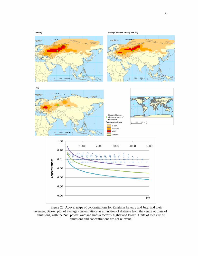
Figure 28: Above: maps of concentrations for Russia in January and July, and their

average; Below: plot of average concentrations as a function of distance from the centre of mass of emissions, with the “4/3 power law” and lines a factor 5 higher and lower. Units of measure of

emissions and concentrations are not relevant.

34

Figure 29: Above: maps of concentrations for Eastern South America in January and July, and their average; Below: plot of average concentrations as a function of distance from the centre

of mass of emissions, with the “4/3 power law” and lines a factor 5 higher and lower. Units of measure of emissions and concentrations are not relevant.

35

Figure 30: Above: maps of concentrations for Europein January and July, and their average; Below: plot of average concentrations as a function of distance from the centre of mass of

emissions, with the “4/3 power law” and lines a factor 5 higher and lower. Units of measure of emissions and concentrations are not relevant.

36

Figure 31: Above: maps of concentrations for Middle East in January and July, and their average; Below: plot of average concentrations as a function of distance from the centre of mass of


37

Figure 32: Above: maps of concentrations for China in January and July, and their



38

Figure 33: Above: maps of concentrations for Northern Africa in January and July, and their average; Below: plot of average concentrations as a function of distance from the centre of


39

Figure 34: Above: maps of concentrations for Northern South America in January and

July, and their average; Below: plot of average concentrations as a function of distance from the centre of mass of emissions, with the “4/3 power law” and lines a factor 5 higher and lower. Units

of measure of emissions and concentrations are not relevant.

40

Figure 35: Above: maps of concentrations for South East Asia in January and July, and

their average; Below: plot of average concentrations as a function of distance from the centre of mass of emissions, with the “4/3 power law” and lines a factor 5 higher and lower. Units of

measure of emissions and concentrations are not relevant.

41

Figure 36: Above: maps of concentrations for Northern Southern Africa in January and

July, and their average; Below: plot of average concentrations as a function of distance from the centre of mass of emissions, with the “4/3 power law” and lines a factor 5 higher and lower. Units

of measure of emissions and concentrations are not relevant.

42

Figure 37: Above: maps of concentrations for Southern Asia in January and July, and their



43

Figure 38: Above: maps of concentrations for Southern Asia in January and July, and their



44

Figure 39: Above: maps of concentrations for Turkey in January and July, and their



45

Figure 40: Above: maps of concentrations for the United States in January and July, and their average; Below: plot of average concentrations as a function of distance from the centre of


46

Figure 41: Above: maps of concentrations for Western Africa in January and July, and their average; Below: plot of average concentrations as a function of distance from the centre of


47

Figure 42: Above: maps of concentrations for Western South America in January and July, and their average; Below: plot of average concentrations as a function of distance from the centre

of mass of emissions, with the “4/3 power law” and lines a factor 5 higher and lower. Units of measure of emissions and concentrations are not relevant.

48

Figure 43: Above: maps of concentrations for Central Asia in January and July, and their average; Below: plot of average concentrations as a function of distance from the centre of mass of


49

4. Implications for global scale comparative chemical risk assessment: an example about the variability of impacts due to the location of the emission

A concern exists about the effects of the spatial variability of the environment on

the predicted impacts of an emission. The availability of simple models such as the onepresented here enable to cope with the spatial distribution of receptors (population or ecosystems or resources) exposed to chemicals, capitalizing on the wealth of data available and without embarking in overly complex and lengthy numerical calculations, if one is interested in a first level of approximation, typically a factor 5 on concentrations, as accepted in many risk assessment contexts.

We shortly present an example here of assessment referred to an atmospheric emission. Further and more comprehensive examples may be developed with reference to different media and emission scenarios, but the example presented here clarifies general concepts essential in the development of guidelines on when one should consider the relevance of spatial variability on the prediction of impacts from chemical pollutants.

Let’s consider a chemical emission to the atmosphere. If one adopts the approximation proposed by Pistocchi and Galmarini, 2008, the spatial distribution of atmospheric concentrations from a constant emission occurring over a limited area may be described with the simple hyperbolic expression as:

C ~ x-4/3. The equation applies to a certain distance from the source, while near the source

concentrations may be approximated through a box model calculation. The impacts of a given concentration on human health are often evaluated using a

linear model. In this case, an impact is proportional to the concentration itself, and to the total population exposed to the concentration. Disregarding proportionality constants, an impact would be calculated for a one-dimensional spatial domain as:

I’ ~ ∫∞

0

)()( dxxCxP

where P(X) and C(x) represent population at distance x from the source, and concentration at the same distance.

In practice, one may define an indicator of impact as follows: I = P0 C0 + P1 C1 + P2 C2 + … where P0 represents the total population exposed to concentration C0 in the area

where the emission occurs; P1 population within a first range of distance from the source, where concentration is C1 ; P2 population within a second range of distance, where concentration is C2; etc. In practice, after a certain distance concentrations become negligible and do not add much to the overall impact.

When referring to normalized concentrations, according to the hyperbolic model of concentration mentioned above, if C0 =1, then C1=(x1/x0)4/3, C2=(x2/x0)4/3 etc.; i.e., for each distance x1,x2, …, we can define a relative concentration to which population is exposed, with reference to the exposure at the source. Weights for the proposed approach depend on distance from the source (Figure 44).

50

0.00

0.20

0.40

0.60

0.80

1.00

1.20

0 50 100 150 200 250 300

Distance (m)

Impact

Figure 44 – weighting function of the concentration with distance

Starting from a map of population distribution, as the gridded population of the

world (GPW) product (http://sedac.ciesin.columbia.edu/gpw/), it is possible to estimate, for each area of emission, both local population and population within a given range from the area of emission.

We decided to refer to a resolution of 0.5o x 0.5o. The local population is obtained by sum-aggregation, to the given spatial resolution, of the original GPW data. The population from 0 to 1 degrees distance from the source is estimated with a neighborhood operation – sum with a 3 x 3 kernel (P3x3); the one from 0 to 1.5 degrees as the latter, but with a 5x5 kernel (P5x5); etc.

All operations are performed using ArcGIS 9.3 – ArcView Spatial Analyst from ESRI. All details on the operators can be found on the documentation quoted in the online help of the software. Then, for each 0.5o x 0.5o cell, the following calculation is performed:

I= ii

iCP∑=

10

1 (*)

Where - P1=population at the cell; - for i=1:10, Pi = P(2i-1)x(2i-1) – Pi -1

and Ci is an appropriate weight, which is given for i=1:10 in Table 1 as derived

from the hyperbolic distribution of concentrations.

51 Weight Orientative

distance from source (km)

Value

C1 50 1 C2 150 0.23112 C3 250 0.116961C4 350 0.07468 C5 450 0.053417C6 550 0.040877C7 650 0.032715C8 750 0.027032C9 850 0.022877C10 950 0.019724

Table 1 – weights for concentration depending on distance

The results of the above described calculation of I for the globe are presented in

normalized scale, and on a logarithmic scale, in Figure 45. the figure needs to be readas follows:

- a value of one (logarithm = zero) means the maximum expected impact I on global scale; this corresponds to the maximum distance-weighted summation of population near the source (equation (*));

- values above -0.5 (logarithm) represent areas with the highest impact an emission placed thereby would have;

- values with decreasing value (down to well below -4) represent areas with decreasing value of the potential impact. In the calculation, it is of course assumed that the emission would have the same

intensity at each location. From the map of Figure 45, it appears that the same emission to the atmosphere would have an

impact varying over more than 4 orders of magnitude, depending on the location of occurrence.

This simple calculation shows that, for the assessment of impacts from a given emission of chemicals, the place where the emission occurs may have a dramatic relevance. This has been shown on the basis of a simple linear model of impact, but is suspected to hold also in the case of more complex, nonlinear models.

In this example, the variability of impacts depends on the variability of population only, as it is assumed that the atmospheric distribution of an emission is the same everywhere. It is clear that this is not realistic. However, experience shows that usually the variability of fate among different places is not so high for a given emission (Hollander et al., 2009). This suggests that, for preliminary assessment, the evaluation of fate for a given chemical may be conducted by neglecting the spatial variability of environmental parameters, while the calculation of impacts of an emission from a limited area cannot be conducted disregarding the local conditions of population. The reasoning presented for population may be extended to other receptors, and particularly to ecosystems, in a straightforward way.

Figure 45 – variability of the impact on population due to an emission to the atmosphere.

53

5. Acknowledgements The HySPLIT analysis setup and development has been conducted by Paolo Isoardi of Reggiani spa, Italy, under a framework contract with the European Commission JRC. Paolo was the authors of the scripts used for the processing of the lights at night and HySPLIT data, as mentioned in the text. The analysis of concentrations as a function of distance, and the evaluation of the variability of impacts described in the example application were conducted by Grazia Zulian of Reggiani spa, Italy, under a framework contract with the European Commission JRC. Grazia also designed the cartography for the analyses of HySPLIT results and coded the scripts for the calculation of geodetic distances. Alberto Pistocchi ideated and designed the research and the analyses and supervised the activities as the technical responsible and project manager of the contracts with Reggiani spa, Italy. Stefano Galmarini and Slawomir Potempski of the Institute for Environment and Sustainability provided comments, discussion and practical tips that helped the setup of the HySPLIT simulations. The example presented in chapter 4 of the report was inspired by discussion with JRC colleagues of the ENSURE action who deal with LCIA, David Pennington and Rana Pant.

6. References

• Draxler, R. R. and Hess, G. D., 1997. Description of the HySPLIT_4 modeling system. NOAA Technical Memorandum ERL ARL-224, Dec, 24p.

• Draxler, R. R., Stunder, B., Rolph, G., Taylor, A., 2008. HySPLIT 4 User’s Guide, version 4.8, February 2008. NOAA Technical Memorandum ERL ARL-230

• EC (2004) European Union System for the Evaluation of Substances 2.0 (EUSES 2.0). Prepared for the European Chemicals Bureau by the National Institute of Public Health andthe Environment (RIVM), Bilthoven, The Netherlands (RIVM Report no. 01900005). Available via the European Chemicals Bureau, http://ecb.jrc.it

• EC, 2003, Technical Guidance Document in support of Commission Directive 93/67/EEC on Risk Assessment for new notified substances, Commission Regulation (EC) No 1488/94 on Risk Assessment for existing substances and Directive 98/8/EC of the European Parliament and of the Council concerning the placing of biocidal products on the market. (http://ecb.jrc.it )

• Elvidge, C. D., Imhoff, M. L., Baugh, K. E., Hobson, V. R., Nelson, I., Safran, J., Dietz, J. B., Tuttle, B. T., 2001. Night-time lights of the world: 1994–1995. ISPRS Journal of Photogrammetry and Remote Sensing, Volume 56, Issue 2, December 2001, Pages 81-99

• Hollander, A., Hauck, M., Cousins, I.T., Huijbregts, M.A.J., Pistocchi, A., Ragas, A.M.J., van de Meent, D., Evaluating the utility of spatiallyexplicit multimedia fate models, submitted, Science of the Total Environment, 2009

• Pistocchi, A. (2008) Fate and Transport models . In Encyclopedia of Quantitative Risk Assessment and Analysis – Melnick, E., Everitt, B. (eds), John Wiley and Sons, Chichester, UK, pp 705-714

• Pistocchi, A., Galmarini, S., Evaluation of a Simple Spatially Explicit Model of Atmospheric Transport of Pollutants in Europe, Environmental Modeling and

54 Assessment, accepted 2008; published online with DOI 10.1007/s10666-008-9187-x http://www.springerlink.com/content/t6682623kl5g22v1/

• Roemer, M., Baart, A., Libre, J.M., ADEPT: development of an Atmospheric Deposition and Transport model for risk assessment, TNO report B&O- A R 2005-208, Apeldoorn, 2005

• Vincenty, T., Direct and Inverse Solutions of Geodesics on the Ellipsoid with application of nested equations, Survey Review, vol XXII no 176, 1975 (available online at http://www.ngs.noaa.gov/PUBS_LIB/inverse.pdf)

European Commission EUR 24264 EN – Joint Research Centre – Institute for Environment and Sustainability Title: An evaluation of the global patterns of atmospheric transport for regionalized chemical risk assessment Author(s): Alberto Pistocchi, Grazia Zulian, Paolo Isoardi Luxembourg: Publications Office of the European Union 2010 – 54 pp. – 21 x 29.7 cm EUR – Scientific and Technical Research series – ISSN 1018-5593 ISBN 978-92-79-15063-0 doi:10.2788/65179 Abstract The report illustrates a research conducted using the HySPLIT chemical atmospheric transport model and the distribution of stable lights at night, to investigate the spatial patterns of atmospheric concentrations from continuous emissions spatially distributed as population. The analysis shows that a first approximation of the spatial distribution of concentrations may be obtained using the simple “4/3 power law” that Pistocchi and Galmarini, 2008, have shown to be able to approximate the plumes of annual average concentration depicted by the European model ADEPT. This finding enables to perform regional risk assessment taking into account the spatial distribution of receptors around, and not just at, the location of emissions, without the need to use complex transport numerical model, if one is interested in a first level of approximation (i.e., a factor 5 accuracy on concentrations, which is often compatible with the requirements of risk assessment). In such circumstances, the “4/3 power law” enables quick and simple back-of-the-envelope calculations, operationally equivalent to simple box model calculations.

How to obtain EU publications Our priced publications are available from EU Bookshop (http://bookshop.europa.eu), where you can place an order with the sales agent of your choice. The Publications Office has a worldwide network of sales agents. You can obtain their contact details by sending a fax to (352) 29 29-42758.

The mission of the JRC is to provide customer-driven scientific and technical support for the conception, development, implementation and monitoring of EU policies. As a service of the European Commission, the JRC functions as a reference centre ofscience and technology for the Union. Close to the policy-making process, it serves the common interest of the Member States, while being independent of specialinterests, whether private or national.

LB-N

A-24264-EN

-C

an evaluation of the global patterns of atmospheric -...

Documents