An Evaluation of the utility of two classifiers for mapping woody vegetation using remote sensing

Silvana Acevedo and Simon Jones

School of Mathematical and Geospatial Sciences RMIT University, Melbourne

Silvana Acevedo: Senior Scientist /GIS analyst at the Department of Sustainability and Environment. Simon Jones: This research was completed as part of Silvana Acevedo’s Master of Applied Science (Geospatial Information) through RMIT University.

Abstract

Native vegetation is vulnerable to fragmentation and loss of condition due to various environmental and anthropogenic drivers. Regrowth can vary depending upon species composition within that vegetation community. As well as maintaining biodiversity native vegetation provides a range of ecosystem services. Up-to date and reliable information on the distribution of native vegetation is essential to support decisions that minimise loss of biodiversity and maximise functionality of ecosystems. Remotely sensed data is an ideal tool for this purpose. As such, this study aims to assess the accuracy of Maximum Likelihood Classification (MLC) and Spectral Angle Mapper (SAM) algorithms to distinguished woody vegetation from non-woody vegetation in Creswick, Victoria, Australia. The use of RapidEye imagery, image fusion (spectral information combined with textual information (ALOS-PALSAR)), and the use of a filter (majority filter) was also evaluated. The classification accuracy of MLC and SAM was used as the determining factor for identifying a suitable mapping method to distinguish woody native vegetation from non-native woody vegetation (particularly, Pinus spp., Pine and Eucalyptus spp., Blue Gum) in the forest.

The results demonstrated that the use of MLC on RapidEye imagery enabled the Native, Pine and Blue Gum to be accurately mapped with an overall accuracy of 88%. Kappa statistics show that there was a significant difference between MLC and SAM algorithms independent of the image type input. However, when the same algorithm was applied on each image type, no significant difference was found. The use of fused images as well as a filter, did not improve the accuracy of the classification. Considering cost and time in registering and processing the images as well as the computational time of images filtering, the use of these methods does not provide benefit in this case study. Key words: woody/non-woody vegetation, classification, data fusion, majority filter, remote sensing

Introduction Native vegetation is part of a dynamic system that must regenerate and mature in order to support biodiversity. Over many thousands of years indigenous flora and fauna have developed and adapted together and are reliant on each other for pollination and habitat. As well as maintaining biodiversity native vegetation cleans the air, filters water, stabilises the soil, and provides a range of ecosystem services. Since settlement, approximately half of Victoria’s native vegetation has been cleared for agricultural and urban development, including 80% of the original cover on private land (DSE 2008). The native vegetation that remains in Victoria is critical for maintaining catchment and landscape health, and protecting the habitats of threatened flora and fauna. In 2008 the Australian states and territories governments reviewed the National Framework for the Management and Monitoring of Australia’s Native Vegetation (published in 1999; ANZECC 1999) which

outlines a coordinated national approach to native vegetation management (DNRE 2002). The Framework addresses native vegetation management from a whole of catchment perspective but necessarily focuses on private land where the critical issues of past clearing and fragmentation exist. The framework identifies that retention and management of remanent native vegetation is the primary way to conserve the natural biodiversity across the landscape (DNRE 2002). Current and accurate information on the distribution of native vegetation is essential to ensure the conservation of biodiversity as well as for preparation and management bushfire hazard. Detailed mapping of native vegetation of Victoria is available in the form of Ecological Vegetation Class (EVC) mapping. EVC represents the highest level in the hierarchical vegetation typology used across Victoria (DSE 2008). EVCs consist of one or more floristic communities that exist under a common regime of ecological processes within a particular environment at a regional, state or continental scale (Woodgate et al 1994). Floristic community differences within EVCs are often geographically or geologically driven. The EVC maps are based on data collected in 2005. Changes in vegetation distributions may be rapid; therefore, we need to be able to report the dynamic nature of the extent and type of woody vegetation. Remotely sensed data is ideal for this purpose. The present study aims: (i) to assess the accuracy of two algorithms, Maximum Likelihood Classification (MLC) and Spectral Angle Mapper (SAM) to distinguished native woody vegetation from non-native vegetation (Pinus (Pine) and Eucalyptus (Blue Gum)), (ii) to reliably distinguish Pine plantations from Blue Gum plantations (iii) to assess the value of using a classification filtering and, (iv) to assess the value of using as an input image spectral information (RapidEye image) and a fusion of image (spectral information combined with backscater information (PALSAR-ALOS)).

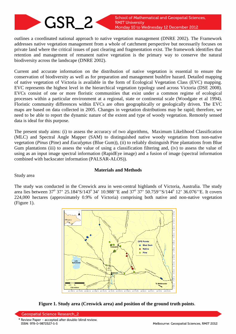
Materials and Methods Study area The study was conducted in the Creswick area in west-central highlands of Victoria, Australia. The study area lies between 37o 37’ 25.184’S/143o 34’ 10.988’’E and 37o 37’ 50.759’’S/144o 12’ 36.076’’E. It covers 224,000 hectares (approximately 0.9% of Victoria) comprising both native and non-native vegetation (Figure 1).

Figure 1. Study area (Creswick area) and position of the ground truth points.

Source of data Ground truth data on the Creswick area was collect on the 23rd of August 2011. A handheld Global Positioning System (GPS) (mode Garmin GPS 72) was used to collect coordinates of individual Native, Blue Gum and Pine trees. A total of 40 samples were collected for each tree. The GPS data collected was divided into two groups. The first group was used as training data for classification of images and the second group (approximately 20 samples for each tree) was later used for validation of the data through accuracy assessment. Two types of images were used in this study: RapidEye (a mosaic of two images; 5 m spatial resolution) and Advanced Land Observing Satellite-Phased Array type L-band Synthetic Aperture Radar (ALOS-PALSAR; HH, HV and HH/HV images; 25 m spatial resolution). The RapidEye images were acquired on the 28th of October 2010 and 13th of March 2010. The ALOS-PALSAR images were acquired between June and September 2009. Analysis of the data Two vegetations indices were calculated in the RapidEye image: Normalised Difference Vegetation Index (NDVI) (Jensen 1986) and a Modified Red Edge Index (REI) (ratio along the red edge (750 and 705 nm) and a correction for scattering light using the blue wavelengths (Tucker 1979). Each ALOS-PULSAR image was re-sampling from 25 m pixel size to 5 m pixel size. In order to maximise the information content of the classifications, the RapidEye (1-5 bands), NDVI and REI (spectral information), ALOS-PULSAR (HH, HV, HH/HV) images were fused together into a single image. The resulting image was then use in the classification. The RapidEye image and the fused images were classified using two supervised classifiers Maximum Likelihood Classification (MLC) (Shafri et al 2007) and Spectral Angle Mapper (SAM) (De Carvalho & Meneses 2000). The MLC classifier assumes that the statistics for each class in each band are normally distributed and calculates the probability that a given pixel belongs to a specific class. Unless a probability threshold is selected, all pixels are classified (in this study no threshold was selected). Each pixel is assigned to the class that has the highest probability. If the highest probability is smaller than a threshold, the pixel remains unclassified. The MLC was calculated based on the formula described on Shafri et al (2007). Whereas SAM, is a physically based spectral classification that uses and n-dimensional angle to match pixels to reference spectral. The algorithm determines the spectral similarity between two spectral by calculating the angle between the spectral and treating them as vectors in a space with dimensionality equal to the number of bands (Kruse et al. 1993). SAM was calculated based on the formula described by De Carvalho & Meneses (2000). The training data was used to develop spectral signatures or Regions of Interest (ROI). The ROIs were then used to train the computer to recognize the different trees on the RapidEye. The spectral separability of the ROIs was calculated using the average of the Transformed Divergence and Jeffries-Matusita separability measures (DIP 2012).

Post-classification The salt and pepper noise of the classified images was removed using a 3x3 kernel size filter. This resulted in an affective Minimum Mapping Unit of 225 m2. Accuracy assessment was assessed using two methods: Confusion Matrix and Kappa Coefficient (± confidence interval) (Senseman et al 1995). Kappa interpretation strength of agreement between two data sets was based on Landis and Koch (1977) guides (values ≤ 0.2 implies poor agreement and values ≥ 0.80 implies very good agreement). Genderen and Lock (1977) states that a minimum sample size of 20 per class is required for a 85% classification accuracy hence, this was set as the minimum acceptable overall accuracy.

The difference in accuracy levels for MLC and SAM on the RapidEye and fused images was computed to test the null hypothesis that there were no significant differences between Kappa 1 and Kappa 2.

Results

Classification ROIs used for classification were ≥ 1.8 and this was considered adequate separability to be discriminate by classification. MLC (prior and post-classification filtering) identified Blue Gum to cover the largest area in the RapidEye image contrary; on the fused images Pine was found to cover the largest area (Figures 2 and 3a,b). In the RapidEye image, Blue Gum covers an area of 18,322 ha, Pine covers an area of 14,760 ha and Native covers an area of 2,677 ha (Figures 2 and 3a). After the filter, Blue Gum and Pine cover a slightly larger area whereas Native covers a slightly smaller area (Figure 2). In the fused images, Pine covers an area of 26,236 ha, Native covers an area of 13,319 ha and Blue Gum covers an area of 4,218 ha (Figures 2 and Figure 3b). After the filter, Pine covers a slightly larger area whereas Native and Blue Gum cover a slightly smaller area (Figures 2).

Figure 2. Area (in hectares) cover by Blue Gum, Native and Pine classes. Shaded areas represented the areas after applying a kernel size of 3x3 filter (majority analysis). Unlike MLC, SAM (prior and post classification filtering) identified Native to cover the largest area and Pine to cover the least (Figure 2 and 3c,d). In the RapidEye image, Native cover an area of 32,029 ha, Blue Gum cover an area of 22,192 ha and Pine an area of 4,700 ha (Figures 2 and 3c). After the filter, both Native and Blue Gum covers slightly larger areas whereas Pine covers a slightly smaller area (Figure 2). In

0

5000

10000

15000

20000

25000

30000

35000

. .

0

5000

10000

15000

20000

25000

30000

35000

RapidEyeClassif

RapidEyeFilter

FusedClassif

FusedFilter

RapidEyeClassif

RapidEyeFilter

FusedClassif

FusedFilter

Area

(hec

tare

s)

Blue Gum Native Pine

MLC SAM

0

5000

10000

15000

20000

25000

30000

35000

. .

0

5000

10000

15000

20000

25000

30000

35000

RapidEyeClassif

RapidEyeFilter

FusedClassif

FusedFilter

RapidEyeClassif

RapidEyeFilter

FusedClassif

FusedFilter

Area

(hec

tare

s)

Blue Gum Native Pine

MLC SAM

the fused images, Native covers an area of 23,572 ha, Blue Gum an area of 13,052 and Pine an area of 1,947 (Figures 2 and 3d). After the filter, the three classes cover a slightly larger area (Figures 2).

Figure 3. Output of Maximum Likelihood Classification (MLC) and Spectral Angle Mapper (SAM).

Accuracy assessment Of 47,659 pixels classified using MLC, 88% and 85% pixels were correctly classified on the RapidEye and the fused images respectively. The filter did not improve the overall accuracy. For both the RapidEye and the fused images, kappa showed a complete agreement between the classified and the reference data (Table 1).

Table 1. Overall accuracy and Kappa coefficient results. Lower limit Observed Upper limit

Image Classifier % Overall accuracy

.95 Confidence interval

Kappa .95 Confidence interval

RapidEye MLC 88 0.841 0.845 0.848 Fused MLC 85 0.815 0.821 0.825 RapidEye SAM 53 0.528 0.533 0.538 Fused SAM 79 0.748 0.752 0.757

After filter RapidEye MLC 87 0.800 0.851 0.854 Fused MLC 85 0.824 0.828 0.832 RapidEye SAM 64 0.584 0.5895 0.594 Fused SAM 78 0.742 0.752 0.756

In the RapidEye image, 99% pixels were correctly classified as Blue Gum. Similarly, 97% pixels were correctly classified as Native and 98% pixels were correctly classified as Pine (producer’s accuracy). The reliability of a pixel labelled as Blue Gum on the classified image actually being Blue Gum in situ is 97%. Likewise, the reliability of the Native classification was 99% and that of the Pine was also 99%. The classification however excluded pixels from the categories in which they belong. For instance, 1.08% pixels were excluded from Blue Gum class, 2.79% pixels were excluded from Native class and 1.83% pixels were excluded from Pine class (errors of omission). Some pixels were ‘included’ in categories in which they do not belong. For instance, 3.04% pixels were included erroneously in the Blue Gum class, 0.73% pixels were included erroneously in the Native class and 0.98% pixels were included erroneously in the Pine class (errors of commission) (Table 2). In the fused image, 99% pixels were correctly classified as Blue Gum. Similarly, 94% pixels were correctly classified as Native and ~100% were correctly classified as Pine (producer’s accuracy). The reliability of a pixel labelled as Blue Gum on the classified image actually being Blue Gum in situ is ~100%. Likewise, the reliability of the Native classification was 99% and that for the Pine was also 99%. The classification however excluded pixels from the categories in which they belong. For instance, 1.08% pixels were excluded from Blue Gum class, 6.24% pixels were excluded from Native class and 0.09% pixels were excluded from Pine class (errors of omission). Some pixels were ‘included’ in the categories in which they do not belong. For instance, 0.14% pixels were included erroneously in the Blue Gum class, 0.60% pixels were included erroneously in the Native class and 0.55% pixels were included erroneously in the Pine class (errors of commission) (Table 2). Of 47,659 pixels classified using SAM, 53% and 78% were correctly classified in the Rapid Eye and the fused images respectively. The filter did not improve the overall accuracy on the fused image but did improve 11% on the RapidEye image. For the RapidEye image, kappa showed that there was a moderate agreement between the classified and the reference data. For fused image, Kappa showed good agreement between the two data sets (Table 1). In the RapidEye image, 96% pixels were correctly classified as Blue Gum. Similarly, 91% pixels were correctly classified as Native and 83% were classified as Pine (producer’s accuracy).The reliability of a pixel labelled as Blue Gum on the classified image actually being Blue Gum is situ is 77%. Likewise, the reliability of the Native classification was 96% and that of the Pine was 97%. The classification however ‘excluded’ pixels from the categories in which they belong. For instance, 4.33% pixels were excluded from Blue Gum class, 9.18% pixels were excluded from Native class and 16.15% pixels were excluded from Pine class (errors of omission). Some pixels were included in the categories in which they do not belong. For instance, 22.71% pixels were included erroneously in the Blue Gum class, 4.44% pixels were included erroneously in the Native class and 3.06% pixels were included erroneously in the Pine class (errors of commission) (Table 2). In the fused image, 84% pixels were classified as Blue Gum. Similarly, 71% pixels correctly classified as Native and 93% were correctly classified as Pine (producer’s accuracy). The reliability of a pixel labelled as Blue Gum on the classified image actually being Blue Gum in situ was 89%. Likewise, the reliability of the Native classification was 73% and that of the Pine was 100%. The classification however excluded pixels from the categories in which they belong. For instance, 15.97% pixels were excluded from Blue Gum class, 0.28% pixels were excluded from Native class and 6.67% pixels were excluded from Pine class (errors of omission). Some pixels were ‘included’ in the categories in which they do not belong. For instance, 10.92% were included erroneously in the Blue Gum class, 27.28% were included erroneously in the Native class and 0.1% were included erroneously in the Pine class (errors of commission) (Table 2).

Table 2. Summary of the confusion matrix results (prior to filter).

Image Classifier Class Percentage Omission

Percentage Commission

User's Accuracy (%)

Producer's Accuracy (%)

Rapid Eye MLC

Blue Gum 0.64 3.04 97 99.00 Native 2.79 0.73 99 97.00 Pine 1.83 0.98 99 98.00

Fused images MLC

Blue Gum 1.08 0.14 100 99.00

Native 6.24 0.60 99 94.00 Pine 0.09 0.55 99 100.00

Rapid Eye SAM

Blue Gum 4.33 22.71 77 96.00 Native 9.18 4.44 96 91.00 Pine 16.15 3.06 97 84.00

Fused images SAM

Blue Gum 15.97 10.92 89 84.00 Native 28.56 27.28 73 71.00 Pine 6.67 0.00 100 93.00

Statistical significance Cohen’s Kappa co-efficient was used to report agreement between the different classification approaches and the results are shown in Table 3. From Table 3 it can be seen that a significant difference was found between MLC and SAM, independent of the image type input. There was no significant difference between the RapideEye and the fused images when using MLC as classifier. However, the performance of the MLC was better for the RapidEye image. There were also no significant differences between the RapidEye and the fused images when using SAM as classifier. However, the performance of the SAM was better for the fused images.

Table 3. Comparison of classification accuracies (Kappa coefficient) (prior to filter). Ho: No differences between K1 and K2

Pairs Results

Image Classifier

Vs

Image Classifier p-value At .95% confidence level

RapidEye MLC RapidEye SAM 0.00 Significant difference

RapidEye MLC Fused MLC 0.84 No significant difference

RapidEye MLC Fused SAM 0.00 Significant difference

RapidEye SAM Fused MLC 0.00 Significant difference

RapidEye SAM Fused SAM 0.59 No significant difference

Fused MLC Fused SAM 0.00 Significant difference

Discussion

Accuracy assessment The accuracy assessment of a remote sensing output is one of the most important steps in any classification. Accuracy is considered to be the degree of closeness of results to the values accepted as true (Verbyla & Hammond 1995). Without an accuracy assessment the output or results is of little value. However, cost-

effectiveness and technical simplicity are also key factors determining the usability and applicability of the method (Franklin 2001). Methods that are less expensive and technically simple will always be adopted if the classification accuracies are not significantly different (Congalton & Green 1999). All these factors however will depend on the purpose and financial value of the resources (Hussin & Atmopawiro 2004). Overall accuracy measures the probability of a reference pixel being correctly classified and takes no account for sources of error (errors of omission or commission) (Colgaton & Green, 1991). In the present study, the minimum acceptable overall accuracy was set at 85% across all classes following Anderson et al (1976) and Van Genderen and Lock (1977) recommendation. With reference to this overall accuracy, only the MLC has met this standard while SAM had overall accuracies lower than the standard value set for this study (regardless of the image dataset used). This means that MLC is a better method for distinguishing Native, Pines and Blue Gum forest in the study area than SAM. Is 85% accuracy acceptable? It is impossible to perfectly assess the true class of every pixel. There are a number of issues that may generate errors in a classification (Oslon 2008). For example, one common error is that it is assumed that our ground truth data are perfect (Verbyla & Hammond 1995). If there are any errors in our reference data (such as incorrect class assignment, change in cover type between the time of imaging and the time of field verification), then some of our correctly classified pixels may be incorrectly assessed as being misclassified (Verbyla & Hammond 1995). Olson (2008) state that 85% figure has been replaced by 80% since consumers are willing to accept and pay for this level of accuracy. Campbell (2002) agreed with Olson (2008) but the former suggested that an overall accuracy of 85% is considered standard for land cover mapping. For the purpose of this study, the minimum overall accuracy was set at 85%. Classification accuracy can be expressed in terms of producer’s accuracy and user’s accuracy. Producer's accuracy represents the percentage of a given class that is correctly identified on the map (errors of omission) whilst user's accuracy (or reliability) represents the probability that a given pixel will appear on the ground as it is classed (error of commission) (Colgaton 1999; Senseman et al 1995). The fact that the overall accuracy of the MLC on the RapidEye image and the fused images (88% and 85% respectively) were good, does not mean that each category was successfully classified at that rate (or vice-versa). For instance, the MLC when applied to RapidEye, the highest user accuracy was for Native class while the highest producer’s accuracy was for Blue Gum. In contrast, SAM applied on RapidEye showed an overall accuracy (53%) below the acceptable level set but the algorithm performed well for Blue Gum. Even though the overall accuracy was way below the minimum acceptable of 85%, as a producer of this map, I can claim that 96% of the time a Blue Gum area was identified as such, a user of this map will find that 96% will actually be Blue Gum. Comparison of the performance of the classifiers and the image input (prior to filter) shows a significant difference between MLC and SAM independent of the image type input. However, when the same classification algorithm was applied on each image type, no significant difference was found. The significant differences between the algorithms used (hence classification accuracies) might have been due to the method of training the classifier. This is because MLC and SAM have different approaches in selecting the training samples for the classification and this may have an influence on the classification accuracies. For instance, MLC quantitatively evaluates both the variance and covariance of the category spectral response patterns when classifying an unknown pixel. It is assumed that the distribution of the cloud of points forming the category training data is normally distributed (Gaussian distribution) (Richards 1999); which was the case for Native, Pine (all 5 bands) and Blue Gum (band 4 (NIR)).

Contrary to MLC, SAM uses the angular information to identify pixel spectra. SAM is based on the idea that an observed reflectance spectrum can be considered as a vector in a multidimensional space, where the

number of dimensions equals the number of spectral bands. If the overall illumination increases or decreases (due to the presence of a mix of sunlight and shadows), the length of this vector will increase or decrease, but its angular orientation will remain constant. If the pixel spectra from the different classes are well distributed in feature space there is a high likelihood that angular information alone will provide good separation (Richard 1999).

From the results it is clear that the data derived from the RapidEye classification has a sufficiently Gaussian distribution to be able to separate Blue Gum from Pine, Blue Gum from Native and Pine from Native, in other words, the data input fulfil the requirement needed for MLC. Conversely, SAM in order to perform optimally may need more information than the direction of a vector to separate the classes under study, which are spectrally difficult to separate. Further, a detailed examination of the spectral signatures (using ROIs separability) shows a good separability between the three classes (pair separation >1.8) which may explain the good performance of MLC.

Image fusion

The information provided by each individual sensor may be incomplete, inconsistent and imprecise for a given application. Image fusion is a process, which creates a new image representing combined information composed from two or more source images. Generally, one aims to preserve as much source information as possible in the fused image with the expectation that performance with the fused image will be better than, or at least as good as, performance with the source images (Leviner & Maltz 2009). However, in the present study, the algorithm used was more important than the image used. Combining different sources of information into a single final result can be expensive and time-consuming. Based on the results, there use of RapidEye image was sufficient to accurately classified Native, Blue Gum and Pines. Classification filtering Classified data often manifest a salt-and-pepper appearance due to the inherent spectral variability encountered by a classification when applied on a pixel-by pixel basis (Congalton 1991). Classification filtering (or smoothing) is an operation to remove speckle noise or isolated pixels in a classified image. These isolated pixels are caused by improper training sample definition or spectral noise in the input image (Nguyen 1997). One means of classification smoothing involves the application of a majority filter (Congalton 1991). In such operations a moving windows is pass through the classified pixel in the window is not the majority class, its identity is changed to the majority class. If there is no majority class in the window, the identity of the centre pixel is not changed. As the windows progresses through the data set, the original class code are continually used, not the labels as modified from the previous window position (Eastman 2006). In the present study, a majority filter was conducted on the classified images and subsequently evaluated using confusion matrix. Comparison of the mapping accuracies between the two classifiers indicated again that MLC has highest classification accuracy than SAM (regardless of the image input). In fact the overall accuracy was 1% lower. SAM applied on RapidEye did improved the overall accuracy (from 53% to 64%); still was way under the minimum level set for this study. Quantitatively, there were no differences in land cover for each class. Filter analysis can be time-consuming (in terms of computational efficiency). It is worthy? It was clear from the results that for the study area, apart from “cosmetic correction” the actual accuracy of the image did not improved.

Conclusions

The classification accuracy of MLC and SAM was used as the determining factor for identifying a suitable mapping method to classified woody native vegetation and non-native vegetation (Pine and Blue Gum) in the Creswick area. Based on the results, it may be concluded that MLC on RapidEye can mapped Native, Pine and Blue Gum with an overall accuracy of 88%, which is above the minimum acceptable overall accuracy of 85%+ set for this study. The use of a combination of data (spectral and textural information) as well as the use of a filter (majority filter), did not improve the accuracy of the classification when using the MLC as a classifier however, the use of fused imagery as well as running a filter over the RapidEye imagery improved SAM performance. Considering cost and time in registering and processing the images as well as the computational time of images filtering, the use of these methods does not provide benefit in this case study when using MLC.

Reference

Anderson, JR Hardy, EE Roach, JT & Witmer, RE 1976, A land use and land cover classification system for use with remote sensor data. Geological Survey Professional Paper 964, USGS, Reston, VA.

ANZCC, 1999, Australia and New Zealand Conservation Council. National Framework for the Management and Monitoring of Australia’s Native Vegetation. Commonwealth of Australia.

Campbell, J 2002, Introduction to Remote Sensing, Guilford Publications Inc., New York, N.Y., pp, 294-333.

Congalton, RG & Green, K 1999, A practical look at the sources of confusion in error matrix generation. Photogrammetric Engineering and Remote Sensing, 59:641-644.

Congalton, RG 1991, A review of assessing the accuracy of classifications of remotely sensed data. Remote Sensing of Environment, 37:35-46.

De Carvalho, OA & Meneses, PR 2000, Spectral Correlation Mapper (SCM): An Improvement on the Spectral Angle Mapper (SAM). Summaries of the 9th Airborne Earth Science Workshop, Publication 00-18, 9 p.

DIP, 2012, Digital Image Processing: A remote Sensing Perspective: Evaluation of training sets (Training Signatures). Viewed August 2012, http://forest.mtu.edu/classes/fw5560/lectures/lecture15%28signatures%29.pdf.

DNRE, 2002, Victoria’s Native Vegetation Management - A Framework for Action. Department of Natural Resources and Environment. 59p. Viewed 16 August 2012, http://www.dse.vic.gov.au/__data/assets/pdf_file/0016/102319/Native_Vegetation_Management_-_A_Framework_for_Action.pdf

DSE, 2008, Native vegetation net gain accounting first approximation report. State of Victoria, Department of Sustainability and Environment, East Melbourne. 26p.

Eastman, JR 2006, IDRISI Andes Tutorial. Clark Labs, Clark University, Viewed 12 June 2012.http://www.geog.ubc.ca/courses/geob373/labs/Andes_Tutorial.pdf

Franklin, SE 2001, Remote Sensing for Sustainable Forest Management. CRC Print ISBN: 978-1-56670-394-9 eBook ISBN: 978-1-4200-3285-7, Viewed 11 August 2012.

Hussin, A & Atmopawiro, VP 2004, Sub-pixel and maximum likelihood classification of Landsat ETM+ images for detecting illegal logging and mapping tropical rain forest cover types in Berau, East Kalimantan, Indonesia. The International Institute for Geoinformation Science and Earth Observation, Enschede, Netherlands.

Kruse, F.A., Boardman, J.W., Lefkoff, A.B., et al. 1993. The Spectral Image Processing System (SIPS): Interactive visualization and analysis of imaging spectrometer data. Remote Sensing of Environment, 44: 145-163.

Landis, JR & Koch, GG 1977, The measurement of observer agreement for categorical data. Biometrics, 33(1): 159–174.

Leviner, M & Maltz M 2009, A new multi-spectral feature level image fusion method for human interpretation. Infrared Physics and Technology, 52:79–88.

Nguyen, DD 1997, Classification smoothing in land cover mapping using MODIS data. Land Degradation and Development, 16:139-149.

Olson, CE 2008, Is 80% accuracy good enough? Pecora 17 – The Future of Land Imaging. Going Operational. November 18-20. Denver, Colorado.

Richards, JA 1999, Remote Sensing Digital Image Analysis: An Introduction. Springer-Verlag, Berlin, Germany, pp. 229-244.

Senseman, GM, Bagley, CF, & Tweddale, SA 1995, Accuracy Assessment of the Discrete Classification of Remotely Sensed Digital Data for Landcover Mapping, USACERL Technical Report EN-95/04, April.

Shafri, HZM, Suhaili, A & Mansor, S 2007, The Performance of Maximum Likelihood, Spectral Angle Mapper, Neural Network and Decision Tree Classifiers in Hyperspectral Image Analysis. Journal of Computer Science, 5(6): 419-423.

Van Genderen, JL & Lock, BF 1977, Testing land use map accuracy, Photogramm Engineering and Remote Sensing, 43(9):1135-1137.

Tucker, C.J., 1979. Red and Photographic Infrared Linear Combinations for Monitoring Vegetation. Remote Sensing of the Environment 8:127-150.

Verbyla, DL & Hammond, TO 1995, Conservative bias in classification accuracy assessment due to pixel-by-pixel comparison of classified images with reference grids. International Journal of Remote Sensing, 16:581-587.

Woodgate, PW, Peel, W, Ritman, KT, Coram, JE, Brady, A, Rule, AJ, & Banks, JCG 1994, A Study of the Old growth Forests of East Gippsland, Conservation and Natural Resources Department, Melbourne.

Acknowledgements

I would like to thank Graeme Newell, Matt White, Peter Griffioen, Bronwyn Price Adrian Kitchingam and Paul Moloney (Department of Sustainability and Environment, Arthur Rylah Institute) for their invaluable help and feedback and for provided me with the images needed to conduct this study and assistance on the collection of ground truth data.

Figure 1.

Figure 2

05000

100001500020000250003000035000

RapidEye_MLC_Classif .

RapidEye_MLC_Filer

Stacked_MLC_Classif .

Stacked_MLC_filter

RapidEye_SAM_Classif

RapidEye_SAM_fiter

Stacked_SAM

Stacked_SAM -

Are

a (h

ecta

res)

Blue Gum Native Pine

Image

0

500010000

15000

20000

25000

3000035000

RapidEyeClassif

RapidEyeFiler

FusedClassif

FusedFilter

RapidEyeClassif

RapidEyeFilter

FusedClassif

FusedFilter

Area

(hec

tare

s)Blue Gum Native Pine

MLC SAM

05000

100001500020000250003000035000

RapidEye_MLC_Classif .

RapidEye_MLC_Filer

Stacked_MLC_Classif .

Stacked_MLC_filter

RapidEye_SAM_Classif

RapidEye_SAM_fiter

Stacked_SAM

Stacked_SAM -

Are

a (h

ecta

res)

Blue Gum Native Pine

Image

0

500010000

15000

20000

25000

3000035000

RapidEyeClassif

RapidEyeFiler

FusedClassif

FusedFilter

RapidEyeClassif

RapidEyeFilter

FusedClassif

FusedFilter

Area

(hec

tare

s)Blue Gum Native Pine

MLC SAM

Figure 3.

Figure 4