an examination and implementation of the libor market · pdf filean examination and...
TRANSCRIPT
An Examination and Implementation of the
Libor Market Model
James Jardine
B.Sc. (Hons) Computer Science & Applied Mathematics
supervised by
Prof. Ronald Becker
Dissertation
presented to the Faculty of Science
of the University of Cape Town
in partial ful�lment of the requirements for the degree of
M.Sc. in the Mathematics of Finance
October 10, 2006

Abstract
The relatively young �eld of quantitative �nance has grown over the past
thirty years with the cherry-picking of a wide variety of techniques from the
disciplines of �nance, mathematics and computer science. The Libor Market
Model, a model for pricing and risk-managing interest rate derivatives, is
a prime example of this cherry-picking, requiring an understanding of the
interest rate markets to understand the problem to be modelled, requiring
some deep mathematics from probability theory and stochastic calculus to
build the model, and requiring a level of computer expertise to e¢ ciently
implement the computationally demanding requirements of the model. This
dissertation intends to draw from a wide literature to bring into one body of
work a treatment of the Libor Market Model from start to �nish.

Contents
1 Introduction 4
2 A brief history of interest rate models 52.1 Instantaneous spot and forward rate models . . . . . . . . . . 5
2.2 Market models . . . . . . . . . . . . . . . . . . . . . . . . . . 7
3 Financial and mathematical foundations 83.1 Simple �nance . . . . . . . . . . . . . . . . . . . . . . . . . . . 8
3.1.1 Tenors and time spans . . . . . . . . . . . . . . . . . . 8
3.1.2 Discount or zero-coupon bonds . . . . . . . . . . . . . 9
3.1.3 Forward continuous discount . . . . . . . . . . . . . . . 10
3.1.4 Forward rate and Libor forward rate . . . . . . . . . . 11
3.1.5 Swap . . . . . . . . . . . . . . . . . . . . . . . . . . . . 13
3.1.6 Coterminal swaps . . . . . . . . . . . . . . . . . . . . . 16
3.1.7 Caplets and caps . . . . . . . . . . . . . . . . . . . . . 17
3.1.8 Swaption . . . . . . . . . . . . . . . . . . . . . . . . . . 18
3.2 Stochastic calculus . . . . . . . . . . . . . . . . . . . . . . . . 18
3.3 General option theory . . . . . . . . . . . . . . . . . . . . . . 24
3.4 Using Black76 to price interest rate options . . . . . . . . . . . 28
3.4.1 Derivation of Black76 for caplets . . . . . . . . . . . . 28
3.4.2 Derivation of Black76 for swaptions . . . . . . . . . . . 30
4 The Libor Market Model 344.1 The plan . . . . . . . . . . . . . . . . . . . . . . . . . . . . . . 34
4.2 Pricing a single caplet . . . . . . . . . . . . . . . . . . . . . . 35
4.3 Pricing more complex instruments . . . . . . . . . . . . . . . . 37
4.4 Discretisation . . . . . . . . . . . . . . . . . . . . . . . . . . . 40
4.5 Pricing �nancial instruments . . . . . . . . . . . . . . . . . . . 43
4.6 Hedging �nancial instruments: the Greeks . . . . . . . . . . . 44
4.6.1 The �nite di¤erence method . . . . . . . . . . . . . . . 47
4.6.2 Other approaches: the pathwise method and the like-
lihood ratio method . . . . . . . . . . . . . . . . . . . . 52
1

5 Model details 535.1 The initial forward rates . . . . . . . . . . . . . . . . . . . . . 53
5.2 Volatility speci�cation . . . . . . . . . . . . . . . . . . . . . . 54
5.3 Correlation speci�cation . . . . . . . . . . . . . . . . . . . . . 58
5.4 Calibration to caplets . . . . . . . . . . . . . . . . . . . . . . . 59
5.5 Calibration to caplets and swaptions . . . . . . . . . . . . . . 61
5.6 Factor reduction . . . . . . . . . . . . . . . . . . . . . . . . . . 66
6 Technical details 686.1 Monte Carlo integration . . . . . . . . . . . . . . . . . . . . . 68
6.2 Random numbers . . . . . . . . . . . . . . . . . . . . . . . . . 70
6.2.1 Pseudo-random numbers . . . . . . . . . . . . . . . . . 71
6.2.2 Quasi-random numbers . . . . . . . . . . . . . . . . . . 72
6.2.3 Antithetics . . . . . . . . . . . . . . . . . . . . . . . . 72
6.2.4 Gaussian draws . . . . . . . . . . . . . . . . . . . . . . 74
6.3 Global optimisation - Nelder-Mead algorithm . . . . . . . . . . 74
6.4 Interest rate derivative products . . . . . . . . . . . . . . . . . 77
6.4.1 Caplet . . . . . . . . . . . . . . . . . . . . . . . . . . . 79
6.4.2 Cap . . . . . . . . . . . . . . . . . . . . . . . . . . . . 79
6.4.3 Limit cap and chooser limit cap . . . . . . . . . . . . . 80
6.4.4 Barrier caplet . . . . . . . . . . . . . . . . . . . . . . . 81
6.4.5 Swaption . . . . . . . . . . . . . . . . . . . . . . . . . . 82
6.4.6 Trigger swap . . . . . . . . . . . . . . . . . . . . . . . 83
6.4.7 Bermudan swaption . . . . . . . . . . . . . . . . . . . . 83
7 Results 847.1 Calibration to caplets . . . . . . . . . . . . . . . . . . . . . . . 84
7.2 Sensitivity of caplet calibration to initial conditions . . . . . . 86
7.3 Calibration to caplets and swaptions . . . . . . . . . . . . . . 89
7.4 Reduced factor matrices . . . . . . . . . . . . . . . . . . . . . 91
7.5 E¤ect of di¤erent random number sources and antithetics . . . 94
7.6 The Greeks . . . . . . . . . . . . . . . . . . . . . . . . . . . . 96
7.7 E¤ect of di¤erent numeraires on accuracy . . . . . . . . . . . . 97
2
7.8 Pricing various options . . . . . . . . . . . . . . . . . . . . . . 100
8 Conclusion 103
9 Bibliography 105
10 Code Appendix 11110.1 Integrating
R ts�i(u)�j(u)du . . . . . . . . . . . . . . . . . . . 111
10.2 Moro�s Normal inverse transform . . . . . . . . . . . . . . . . 112
10.3 The Nelder-Mead algorithm . . . . . . . . . . . . . . . . . . . 113
10.4 The Mersenne Twister algorithm . . . . . . . . . . . . . . . . 120
3

1 Introduction
The relatively young �eld of quantitative �nance has grown over the past
thirty years with the cherry-picking a wide variety of techniques from the
disciplines of �nance, mathematics and computer science. The Libor Market
Model, a model for pricing and risk-managing interest rate derivatives, is
a prime example of this cherry-picking, requiring an understanding of the
interest rate markets to understand the problem to be modelled, requiring
some deep mathematics from probability theory and stochastic calculus to
build the model, and requiring a level of computer expertise to e¢ ciently
implement the computationally demanding requirements of model.
This dissertation intends to draw from a wide literature to bring into one
body of work a treatment of the Libor Market Model from start to �nish.
Careful attention has been paid to ensuring consistency in style and notation
in the material sourced from di¤erent works in the literature. It is intended
that the reader will, by the end of this dissertation, have understood the
basics of the Libor Market Model and be able to go about implementing
a reasonable version of the model for themselves without having to piece
together information from other sources. That said, where one approach
has been chosen over another, references are made to those alternatives in
the literature.
We start in Section 2 with a brief history of the �eld of interest rate
derivative modelling. Section 3 then presents the �nancial background and
mathematical foundation required for the mathematical development of the
Libor Market Model in Section 4. Section 5 goes into the details of the model,
turning the mathematical model into something that can model the market.
Section 6 covers some of the technical details required in the implementation
of the model, mainly topics from computer science but also including the
code for modelling some interest rate derivatives. Section 7 discusses some
results from using the model. We close with Section 8, which summarises
the work done and points to potential areas of further research.
4

2 A brief history of interest rate models
In 1979 the Fed changed their monetary policy from one where interest rates
were historically static quantities to one where interest rates play a vital role
in the steering of economic variables. Since then there has been a consid-
erable increase in the volatility of interest rates inside the USA and around
the world [50]. Market players have become more and more dependent on
interest rate derivatives as vital sources of insurance against adverse moves in
interest rates. This huge increase in demand for interest rate derivatives has
inspired a lot of research into creating new and useful interest rate products
and into how these derivatives should be priced.
This research has spawned a plethora of models that are used as "extrap-
olation tools" to determine the prices of exotic interest rate derivatives, each
with its own set of assumptions and solutions. No model solves all problems:
traders regularly use several similar but inconsistent models to model secu-
rities with the same underlying [17]. Indeed, [65] states that all models he
has ever seen can go wrong under some circumstances: its just a question of
how wrong, and whether or not it is a problem for the pricing task at hand.
The modelling of interest rate derivatives has up to now fallen into two
broad categories: those modelling instantaneous spot and forward rates, rates
which are themselves not visible in the market but can be used to synthesize
market rates; and those modelling rates that are visible in the market, like
Libor and swap rates.
2.1 Instantaneous spot and forward rate models
The �rst category of models contains the spot and forward rate models.
They model an instantaneous interest rate (be it the instantaneous spot rate
or forward rate) to generate the term structure of interest rates. An instan-
taneous rate is the amount of interest one earns on a risk-free investment in
an in�nitesimal amount of time. Because of the simplicity of the underlying,
these models generally have elegant closed form solutions for the instanta-
neous spot rate and forward rates - rates that are mathematical constructs
that do not really exist in the market. However, it becomes quite com-
5

plicated to price real-world instruments like caps and swaptions using these
models. Another problem is that their elegantly simple structure limits their
pricing potential and those few models with a rich analytical structure do
not describe interest rate derivatives very well [50].
These models started emerging in the late 1970s and are still used today
[55]. Although they started as a hodgepodge of di¤erent approaches using
PDEs, equilibrium models and expectations, most have been resolved into
the single HJM framework [24] that prescribes arbitrage free dynamics using
equivalent martingale measures with the risk-free bank account as numeraire.
[28] shows how all forward rate models can be written as a spot rate model.
Although a detailed treatment of the various spot and forward rate models
can be found in [55] and [62], we present a brief chronology of the models that
we feel were signi�cant in leading to the development of the market models
described in the next section, and which form the subject of this dissertation:
� 1977 - the Vasicek model [63] introduces the technique of valuing in-terest rate derivatives using partial di¤erential equations.
� 1985 - the Cox-Ingersoll-Ross model [16] models an equilibrium model
of the economy and then derives bond prices from variables in this
economy.
� 1986 - the Ho-Lee model [25] models the entire yield curve rather thanjust the instantaneous rate.
� 1990 - the Hull-White model [27] adds reversion to a time-dependentdrift. This allows for much simpler calibration of the model to the
initial term structure, allowing the model to correctly price products
in the market.
� 1990 - the Black-Derman-Toy model [6] introduces a discrete timemodel of the term structure.
� 1992 - the Longsta¤-Schwartz model [39] extends the Cox-Ingersoll-Ross model to model the dynamics of the short rate and its instanta-
neous volatility.
6
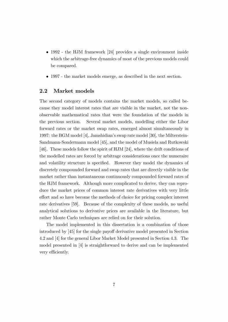
� 1992 - the HJM framework [24] provides a single environment inside
which the arbitrage-free dynamics of most of the previous models could
be compared.
� 1997 - the market models emerge, as described in the next section.
2.2 Market models
The second category of models contains the market models, so called be-
cause they model interest rates that are visible in the market, not the non-
observable mathematical rates that were the foundation of the models in
the previous section. Several market models, modelling either the Libor
forward rates or the market swap rates, emerged almost simultaneously in
1997: the BGMmodel [4], Jamshidian�s swap rate model [30], the Milterstein-
Sandmann-Sondermann model [45], and the model of Musiela and Rutkowski
[46]. These models follow the spirit of HJM [24], where the drift conditions of
the modelled rates are forced by arbitrage considerations once the numeraire
and volatility structure is speci�ed. However they model the dynamics of
discretely compounded forward and swap rates that are directly visible in the
market rather than instantaneous continuously compounded forward rates of
the HJM framework. Although more complicated to derive, they can repro-
duce the market prices of common interest rate derivatives with very little
e¤ort and so have become the methods of choice for pricing complex interest
rate derivatives [59]. Because of the complexity of these models, no useful
analytical solutions to derivative prices are available in the literature, but
rather Monte Carlo techniques are relied on for their solution.
The model implemented in this dissertation is a combination of those
introduced by [45] for the single payo¤ derivative model presented in Section
4.2 and [4] for the general Libor Market Model presented in Section 4.3. The
model presented in [4] is straightforward to derive and can be implemented
very e¢ ciently.
7
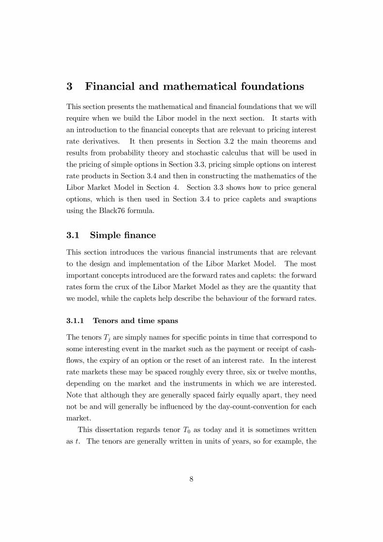
3 Financial and mathematical foundations
This section presents the mathematical and �nancial foundations that we will
require when we build the Libor model in the next section. It starts with
an introduction to the �nancial concepts that are relevant to pricing interest
rate derivatives. It then presents in Section 3.2 the main theorems and
results from probability theory and stochastic calculus that will be used in
the pricing of simple options in Section 3.3, pricing simple options on interest
rate products in Section 3.4 and then in constructing the mathematics of the
Libor Market Model in Section 4. Section 3.3 shows how to price general
options, which is then used in Section 3.4 to price caplets and swaptions
using the Black76 formula.
3.1 Simple �nance
This section introduces the various �nancial instruments that are relevant
to the design and implementation of the Libor Market Model. The most
important concepts introduced are the forward rates and caplets: the forward
rates form the crux of the Libor Market Model as they are the quantity that
we model, while the caplets help describe the behaviour of the forward rates.
3.1.1 Tenors and time spans
The tenors Tj are simply names for speci�c points in time that correspond to
some interesting event in the market such as the payment or receipt of cash-
�ows, the expiry of an option or the reset of an interest rate. In the interest
rate markets these may be spaced roughly every three, six or twelve months,
depending on the market and the instruments in which we are interested.
Note that although they are generally spaced fairly equally apart, they need
not be and will generally be in�uenced by the day-count-convention for each
market.
This dissertation regards tenor T0 as today and it is sometimes written
as t. The tenors are generally written in units of years, so for example, the
8

Figure 1: Tenors Ti and time spans �i.
�rst two tenors, in six months and twelve months, will be written
T1 = 0:5
T2 = 1:0
The time span �j is simply the space of time between tenors Tj�1 and Tjand is de�ned as
�j = Tj � Tj�1
The �j are generally not equal since the tenors are generally not equally
spaced. Figure 1 illustrates tenors and time spans.
3.1.2 Discount or zero-coupon bonds
Discount or zero-coupon bonds are instruments that are bought at less than
face value and at their expiry they pay their face value. This implies that
some interest is earned over the period between paying for the bond and
receiving a larger payment on expiry of the bond. Generally speaking,
these instruments are not traded in their own right, but rather are stripped
from the more common coupon-bearing bonds and interest rate swaps using
methods like those described in [22].
The discount bond P (t; Tj) is the time-t value of the bond with face value
1 expiring at time Tj, i.e. P (Tj; Tj) = 1. Note that if positive interest is
accrued in the market, P (t; Tj) < 1 for t < Tj. Also P (t; Tj) > 0, or we have
arbitrage where zero money at time t is worth 1 at time Tj. Using arbitrage
arguments, P (t; Tj) is the amount by which we multiply any cash�ows arising
at time Tj to calculate their equivalent value today at time t. See [26] for
more details on bond mathematics.
9

Figure 2: The forward continuous discount where a cash�ow of 1 at timeTj�1 is worth Pj(t) =
P (t;Tj�1)P (t;Tj)
at time Tj.
Theorem 1 In an arbitrage-free bond market we have that P (t; Tj�1) >P (t; Tj).
Proof. This proof is adapted from [46]. Suppose, on the contrary, that
P (t; Tj�1) � P (t; Tj). Then purchase one P (t; Tj�1) bond and sell one
P (t; Tj) bond for a positive initial cash�ow. At time Tj�1 we receive 1 unit
cash, which we store (or invest for further pro�t) until time Tj, when we pay
1 unit cash and pocket the interest gained over the period [Tj�1; Tj]. This
is an arbitrage.
Note that if we have zero interest rates then no arbitrage implies only the
weaker P (t; Tj�1) � P (t; Tj).
3.1.3 Forward continuous discount
The forward continuous discount Pj(t) = P (t; Tj�1; Tj) is de�ned as
Pj(t) = P (t; Tj�1; Tj) =P (t; Tj�1)
P (t; Tj)
It is a shorthand notation for calculating the time Tj value of cash�ows
at time Tj�1. Figure 2 shows this relationship: a cash�ow of 1 at time Tj�1is worth P (t; Tj�1) at time t and
P (t;Tj�1)P (t;Tj)
at time Tj. Note that Pj(t) > 1 is
a direct consequence of Theorem 1.
10
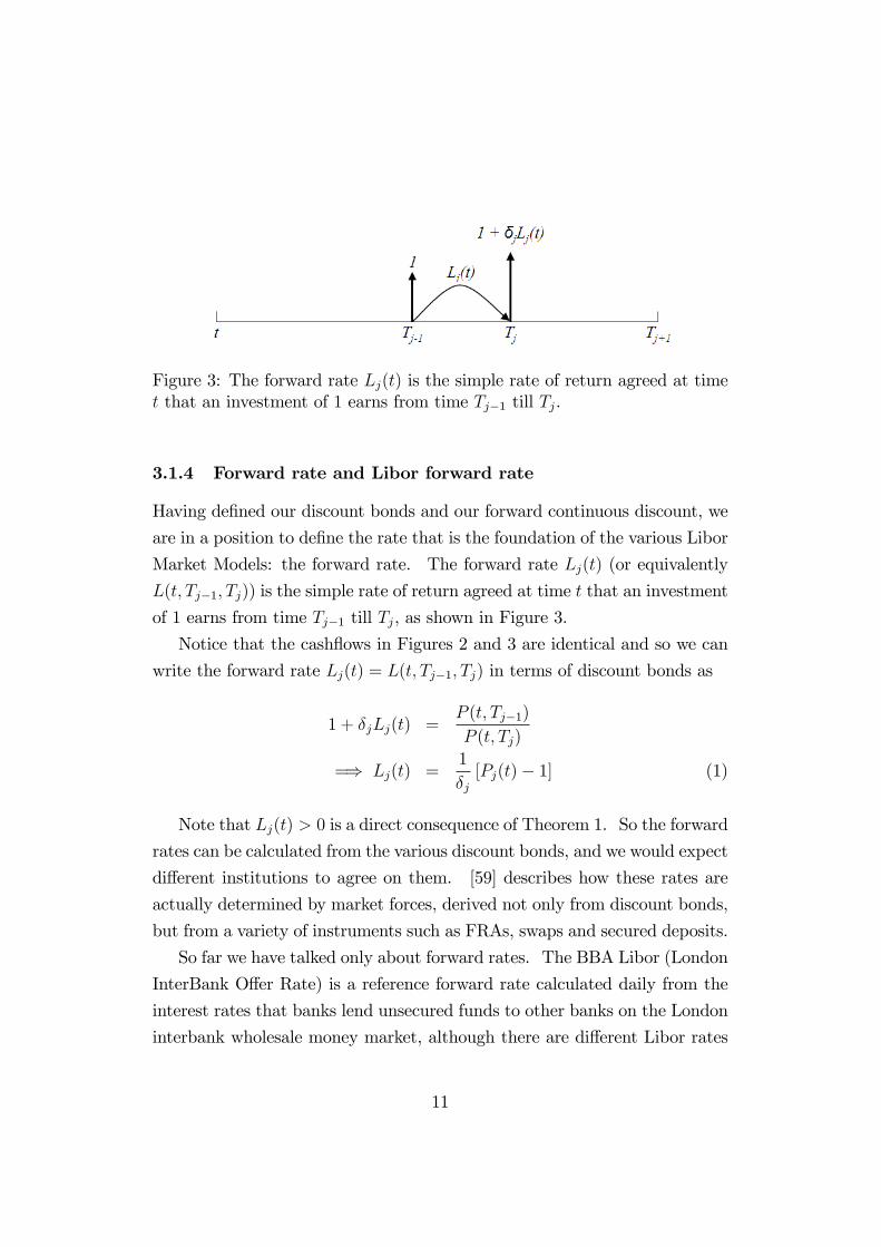
Figure 3: The forward rate Lj(t) is the simple rate of return agreed at timet that an investment of 1 earns from time Tj�1 till Tj.
3.1.4 Forward rate and Libor forward rate
Having de�ned our discount bonds and our forward continuous discount, we
are in a position to de�ne the rate that is the foundation of the various Libor
Market Models: the forward rate. The forward rate Lj(t) (or equivalently
L(t; Tj�1; Tj)) is the simple rate of return agreed at time t that an investment
of 1 earns from time Tj�1 till Tj, as shown in Figure 3.
Notice that the cash�ows in Figures 2 and 3 are identical and so we can
write the forward rate Lj(t) = L(t; Tj�1; Tj) in terms of discount bonds as
1 + �jLj(t) =P (t; Tj�1)
P (t; Tj)
=) Lj(t) =1
�j[Pj(t)� 1] (1)
Note that Lj(t) > 0 is a direct consequence of Theorem 1. So the forward
rates can be calculated from the various discount bonds, and we would expect
di¤erent institutions to agree on them. [59] describes how these rates are
actually determined by market forces, derived not only from discount bonds,
but from a variety of instruments such as FRAs, swaps and secured deposits.
So far we have talked only about forward rates. The BBA Libor (London
InterBank O¤er Rate) is a reference forward rate calculated daily from the
interest rates that banks lend unsecured funds to other banks on the London
interbank wholesale money market, although there are di¤erent Libor rates
11

Figure 4: Synthesizing P (Ti; Tj) discount bonds from the forward rates span-ning from times Ti to Tj.
in many currencies and markets. Practitioners of the Libor Market Model
use the Libor rates of the market to which they have access.
The next theorem gives us the ability to synthesize P (Ti; Tj) discount
bonds from the forward rates spanning from times Ti to Tj. This relationship
is shows graphically in Figure 4.
Theorem 2 Given a set of forward Libor rates, Lk(Ti); k = i + 1 : : : j, we
can calculate the value of P (Ti; Tj) by
P (Ti; Tj) =1
jYk=i+1
(1 + �kLk (Ti))
(2)
Proof.
Pj(Ti) =P (Ti; Tj�1)
P (Ti; Tj)
=) P (Ti; Tj) =P (Ti; Tj�1)
Pj(Ti)=
P (Ti; Tj�2)
Pj(Ti)Pj�1(Ti)= � � �
=P (Ti; Ti)
Pj(Ti)Pj�1(Ti) � � �Pi+1(Ti)
=1
jYk=i+1
Pk(Ti)
12

Now from (1) we have Pj(t) = 1 + �jLj(t), so
P (Ti; Tj) =1
jYk=i+1
(1 + �kLk (Ti))
Note that this formula only holds for Ti falling on a Libor reset date.
For an arbitrary t < Ti we require the existence of an additional bond in the
market P (t; Ti) to calculate P (t; Tj) by
P (t; Tj) = P (t; Ti)P (Ti; Tj)
Now that we have a de�nition for P (t; Tj) and Lj(t) let us brie�y show
that the quantity Lj(t)P (t; Tj) is an asset that is traded in the market. We
will use this fact in Section 4.2 to create ratios between two traded assets,
Lj(t)P (t; Tj) and P (t; Tj).
Lemma 3 Lj(t)P (t; Tj) is a tradable asset.
Proof. From (1) we have
Lj(t) =1
�j
�P (t; Tj�1)
P (t; Tj)� 1�
=) Lj(t)P (t; Tj) =P (t; Tj�1)� P (t; Tj)
�j
Note that Lj(t)P (t; Tj) can be written as a portfolio of tradable assets, and
is therefore itself tradable.
3.1.5 Swap
Swaps are simply �nancial commitments to exchange one set of cash�ows for
another over a given period of time. They are used primarily in the risk
management of future cash�ows, examples of which are covered in [26]. In
our case we are interested in vanilla interest rate swaps where one counter-
party pays a �xed rate of interest at each period while the other counterparty
13

Figure 5: The cash�ows of a payer swap with �xed rate SRi from period Tito TN .
pays the �oating Libor rate. A payer swap is one that is valued from the
viewpoint of the counterparty paying the �xed rate. Figure 5 shows the
cash�ows of a payer swap with �xed rate SRi from period Ti to TN . Upward
arrows represent positive cash�ows, while downward ones represent negative
cash�ows. Notice that while the negative cash�ows (downward pointing ar-
rows) are at the constant rate SRi the positive cash�ows (upward pointing
arrows) are variable, depending on the Libor rate Li(Ti�1) set at time Ti�1.
We should like to calculate the swap rate SRi that balances the positive
and negative cash�ows. The �xed leg of the swap from time Ti to TN pays
SRi�j at time Tj for j = i : : : N . The present value of all these cash�ows is
V alue�xed = SRi
NXj=i
�jP (Tj)
By converting each of the �oating rates of the swap into a �xed rate using
a FRA (a zero cost structure that locks in future forward rates - see [26] for
details), the �oating leg of the swap pays Lj�j at time Tj for j = i : : : N .
The present value of these cash�ows is
V alue�oating =NXj=i
Lj�jP (Tj)
14

We set these cash�ows equal, yielding
V alue�xed = V alue�oating
SRi
NXj=i
�jP (Tj) =
NXj=i
Lj�jP (Tj)
=) SRi =
NXj=i
Lj�jP (Tj)
NXj=i
�jP (Tj)
=) SRi =NXj=i
wi;jLj (3)
where
wi;j =�jP (Tj)NXk=i
�kP (Tk)
Note thatNXj=i
wi;j = 1
so our swap rate is just a weighted average of our forward rates and so must
always lie between the lowest and highest forward rates.
We have seen that the swap rate SRi is chosen to make the swap initially
worthless. As time passes and the underlying interest rates move with
market pressure, the swap may gain or lose value. Consider if we entered
into a swap at time t at fair swap rate SRi, which initially had zero value.
Lets imagine that at some later time t0 (still before the �rst swap payment)
we wished to enter into the identical swap and found that its fair swap rate
is SR0i. What is the value of our original swap? We follow the argument
presented in [32]. Write the original swap rate as SRi = SR0i+(SRi�SR0i).
15

Then our original swap will be paying on the �xed leg the amount
SRi
NXj=i
�jP (Tj) = [SR0i + (SRi � SR0i)]
NXj=i
�jP (Tj)
= SR0i
NXj=i
�jP (Tj) + (SRi � SR0i)
NXj=i
�jP (Tj)
where the �rst term is the same as what a swap entered into today would pay,
and the second term is some extra payment. Note that the �oating legs will
pay the same amounts. Thus if the �xed leg is paying some extra amount
on top of an initially worthless swap, then the value of the swap entered into
at time t must be equal to the negative of that amount, i.e.
Vi(t) = �(SRi � SR0i)NXj=i
�jP (Tj)
= (SR0i � SRi)NXj=i
�jP (Tj) (4)
We will use Equation (4) when calibrating to swaptions in Section 5.5.
3.1.6 Coterminal swaps
The concept of coterminal swaps is important when we come to calibrate our
Libor Market Model to swaptions in Section 5.5. Coterminal swaps are a
collection of swaps who have di¤erent initial payment dates but identical �nal
payment dates. Figure 6 shows a set of coterminal swaps SRj for j = i : : : N ,
where the �rst cash�ow for swap SRi is at time Ti and �nal cash�ow is at
time TN . As you might imagine, and as will be seen in Section 5.5, given two
consecutive swap rates SRi(t) and SRi+1(t) it should be possible to determine
some of the properties of the one forward rate Li�1(t) in which they di¤er.
Indeed, the entire latter part of the yield curve can be bootstrapped from a
set of coterminal swaps [22].
16

Figure 6: Coterminal swaps are a collection of swaps who have di¤erentinitial payment dates but identical �nal payment dates.
3.1.7 Caplets and caps
A caplet is an option on a forward rate. A caplet capleti pays �i (Li(Ti�1)�K)+
at time Ti. It is generally used to hedge future payments of interest on bor-
rowings: buying a caplet capleti with strike K in the same quantity as the
amount borrowed ensures that the maximum interest payable over the period
from Ti�1 to Ti is capped at the caplet strike K since the caplet would pay
out the same amount as would be incurred by any interest rate higher than
the caplet strike.
Single caplets are not generally traded but rather come in bundles of con-
secutive caplets called caps, designed, for example, to last the same amount
of time as an interest bearing loan. Caplet prices (or implied volatilities) can
be approximately stripped from market cap prices using the various methods
described in [26] or obtained directly from the trading desk. They are gener-
ally priced using the Black76 model with the assumption that the underlying
forward rates are lognormal, as is described in detail in Section 3.4.1.
17

3.1.8 Swaption
A swaption is an option on a swap. The holder of a European call swaption
on a payer swap has the right at option expiry to enter into an underlying
swap at a predetermined (�xed-leg) swap rate. Clearly the option will be
exercised only if the option strike is lower than the prevailing par swap rate at
option expiry. Swaptions are generally priced using the Black76 model with
the assumption that the underlying swap rates are lognormal, as is described
in detail in Section 3.4.2.
A set of coterminal swaptions have corresponding coterminal swaps as
their underlyings. These instruments are used to calibrate the Libor Market
Model to market swaptions, as will be seen in Section 5.5.
3.2 Stochastic calculus
This section presents the main theorems and results from probability theory
and stochastic calculus that will be used in the remainder of the disserta-
tion. Most theorems are stated without proof. Generally, the results from
stochastic calculus can be found in [48] and [44] while the probability theory
is concisely covered in [3].
Let us �rst introduce some de�nitions that are used by several of the
theorems in this section. LetW (t) = (W1(t); :::;Wn(t)) be an n-dimensional
standard Brownian motion and F (n)t be the �-algebra generated by W (t).
Let X(t) be the n-dimensional Itô process of the form
dX(t) = �(t)dt+ �(t)dWt
where X(t), �(t), and dWt are n-dimensional vectors and �(t) is an n � n
matrix.
�(t) is the drift of the stochastic process and is
� F (n)t -adapted
� P
24 tZ0
j�(s)dsj <1 for all t > 0
35 = 118

�(t) is the volatility of the stochastic process and determines the exposure
of X(t) to the underlying Brownian motion, and is (see [48] for technicalities)
� F (n)t -adapted
� càdlàg
� E�Z
k�k2 (s)ds�<1
The �rst three theorems cover the dynamics of a stochastic process. Itô�s
Theorem provides us with the chain-rule equivalent of calculus and allows us
to build up the complex functions of underlying random processes that we
will use to model forward rates. Theorems 5 and 6 show how the stochastic
components of a stochastic process behave under the expectation operator.
We use these when calculating the expected values of our models.
Theorem 4 (Itô�s theorem) Let g(t; x) = (g1(t; x); : : : ; gp(t; x)) be a C2
map from [0;1)�Rn into Rp. Then the process Y (t; !) = g(t;X(t)) is again
an Itô process given by
dYk =@gk@t(t;X)dt+
Xi
@gk@xi
(t;X)dXi+1
2
Xi;j
@2gk@xi@xj
(t;X)dXidXj; k = 1 : : : p
The proof of this theorem can be found in [48].
Theorem 5
EP
24 TZt
�(s)dW (s) j Ft
35 = 0The proof and more rigorous technical speci�cation of this theorem can be
found in [48].
Theorem 6 (The Itô isometry)
EP
2640@ TZ
t
�(s)dW (s)
1A2
j Ft
375 = EP24 TZt
�2(s)ds j Ft
3519

The proof and more rigorous technical speci�cation of this theorem can be
found in [48].
The martingale representation theorem tells us that if we have a martin-
gale process with mild restrictions (and in our case we are going to use the
fact that various ratios of the forward rates �t this description) then that
process can be written as an integral equation of Brownian motion. Once
we are in the world of Brownian motion we have at our disposal the tools of
stochastic calculus.
Theorem 7 (The martingale representation theorem) Suppose Mt is
an F (n)t martingale (w.r.t P) and that Mt 2 L2(P) for all t � 0. Then there
exists a unique previsible stochastic process �(s; !) such that
Mt(!) = E [M0] +
tZ0
�(s; !)dW (s) a:s:, for all t � 0:
The proof and more rigorous technical speci�cation of this theorem can be
found in [48].
A process that is a martingale under one probability measure is generally
not a martingale under a di¤erent equivalent probability measure. Gir-
sanov�s theorem tells us how to change the drift of the process so that it is
again a martingale under the new equivalent probability measure. We will
use this to turn all our forward rate processes into martingales under a single
"terminal" probability measure.
Theorem 8 (Girsanov�s theorem) Let W P be a standard d-dimensional
Brownian motion on (;F ;P; fFgt) and let ', the Girsanov kernel, be anyd-dimensional adapted row vector process. De�ne the process L on [0; T ] by
dLt = 'tLtdWPt (5)
L0 = 1
=) Lt = exp
0@ tZ0
'sdWPs �
1
2
tZ0
k'sk2 ds
1A20

Assume that
EP [Lt] = 1
and de�ne the probability measure Q on FT equivalent to P by
LT =dQdP
=) dQ = LTdP
=) Q(A) =
ZA
LT (!)dP(!); A 2 FT
Then,
dW Pt = 'tdt+ dWQ
t
where WQ is a Q-Brownian motion. That is,
WQt = W P
t �tZ0
'sds
is a Q-Brownian motion. The proof and more rigorous technical speci�cationof this theorem can be found in [3].
By putting an integrability restriction on the Girsanov kernel, the Novikov
condition ensures that things don�t blow up when performing the Girsanov
transform. We will see in Section 4.3 that the kernel we use in the Libor
Market Model is a combination of our forward rates and the discount bonds,
a combination that satis�es the Novikov condition.
Lemma 9 If the Girsanov kernel ' is such that
EP24exp
0@12
TZ0
k'tk2 dt
1A35 <1then Lt de�ned by (5) is a martingale and EP [Lt] = 1. The proof of this
theorem can be found in [3].
The change of numeraire is a powerful technique for valuing derivatives
using the martingale approach to arbitrage pricing theory. We �rst de�ne
21

what a numeraire is, show that an equivalent probability measure does indeed
exist for this numeraire, and then describe how to use them to price arbitrary
derivative products.
De�nition 10 (Numeraire) A numeraire is simply the unit of measure interms of which we �nd the worth of �nancial instruments, be it in terms of
currency, gold, index levels, etc. In arbitrage pricing theory, risk-neutral
valuation uses the risk-free bank account as the numeraire, but pricing prob-
lems can sometimes be signi�cantly simpli�ed by using a di¤erent instrument
as the numeraire. In an arbitrage-free market any traded asset can be used
as a numeraire [23]. The Libor Market Model uses various discount bonds
as numeraire.
Theorem 11 (The First Fundamental theorem) A �nancial model is
arbitrage free i¤ there exists a (local) martingale measure PX (equivalent tothe risk-neutral measure P) for the numeraire X. The proof of this theoremcan be found in [3].
Theorem 12 (General pricing formula) LetX and V be the price processes
of two assets in our �nancial model. Let X be the numeraire with a cor-
responding martingale measure PX . Then the price of V (t) at time t with
arbitrary payo¤ V (T ) at time T can be calculated using
V (t) = X(t)EPX
�V (T )
X(T )j Ft�
The proof of this theorem can be found in [3].
The abstract Bayes theorem allows us to �nd the expectation of a random
variable under a probability measure we know little about by �nding rather
the expectation of the variable under a known equivalent probability measure
but weighted by some known likelihood process. We need it to prove the
theorem that follows.
Theorem 13 (Abstract Bayes theorem) Assume that X is a random
variable on (;F ;P) and let Q be another probability measure on (;F) with
22

Radon-Nikodym derivative L = dQdP on F . Assume that X 2 L1(;F ;Q) and
that G is a �-algebra with G � F . Then
EQ [X j G] = EP [L �X j G]EP [L j G]
; Q-a.s.
The proof of this theorem can be found in [3].
The following theorem helps us choose the likelihood ratio that will gener-
ate a new numeraire�s martingale measure from an existing one. We will use
this result repeatedly to move between the equivalent martingale measures
where each discount bond is the numeraire.
Theorem 14 We have a probability measure P0 for the numeraire S0 andwish to generate a new martingale measure P1 for the numeraire S1. If we
de�ne P1 using Girsanov�s theorem (Theorem 8) with the likelihood process
L10(t) =S0(0)
S1(0):S1(t)
S0(t); 0 � t � T
then P1 is a martingale measure for numeraire S1.
Proof. Consider any arbitrage free price process �. We wish to show thatthe normalised process �(t)=S1(t) is a P1-martingale. Note that �(t)=S0(t)and L10(t) are P0-martingales. For s � t, using the Abstract Bayes theorem
23

(Theorem 13), we have
EP1��(t)
S1(t)j Fs
�=
EP0hL10(t)
�(t)S1(t)
j Fsi
EP0 [L10(t) j Fs]
=EP0
hL10(t)
�(t)S1(t)
j Fsi
L10(s)
=EP0
hS0(0)S1(0)
S1(t)S0(t)
�(t)S1(t)
j Fsi
L10(s)
=EP0
hS0(0)S1(0)
�(t)S0(t)
j Fsi
L10(s)
=S0(0)
S1(0)
EP0h�(t)S0(t)
j Fsi
L10(s)
=S0(0)
S1(0)
�(s)S0(s)
L10(s)
=S0(0)
S1(0)
�(s)
S0(s)
S1(0)
S0(0)
S0(s)
S1(s)
=�(s)
S1(s)
Thus �(t)=S1(t) is a P1-martingale and P1 is a martingale measure fornumeraire S1.
3.3 General option theory
This section presents two important results from stochastic calculus for the
pricing of vanilla European options. The �rst describes the statistical qual-
ities of lognormal processes and the second uses these qualities to obtain a
closed formula for a vanilla European option. For an in-depth treatment of
martingale pricing theory, refer to [23].
Theorem 15 If we have a process with the following dynamics
dL(t) = L(t)�(t)dW (t)
24

where Wt(t) is a standard Brownian motion under some probability measure
P and �(t) is deterministic, then L(T ) is lognormal under P with
V arP [lnL(T ) j Ft] =TZt
k�(s)k2 ds
EP [lnL(T ) j Ft] = lnL(t)� 12
TZt
k�(s)k2 ds
Proof. We have dL(t) = L(t)�(t)dW (t). Put Y (t) = lnL(t). Let us �nd
the P-dynamics for lnL(T ) using Itô:
dY =1
LdL� 1
2
1
L2d hLi
= �12k�(t)k2 dt+ �(t)dW (t)
=) d(lnL) = �12k�(t)k2 dt+ �(t)dW (t)
=) lnL(T ) = lnL(t)� 12
TZt
k�(s)k2 ds+TZt
�(s)dW (s)
Consider the mean of lnL(T ) under P:
EP [lnL(T ) j Ft] = EP
24lnL(t)� 12
TZt
k�(s)k2 ds+TZt
�(s)dW (s) j Ft
35= EP [lnL(t) j Ft] + EP
24�12
TZt
k�(s)k2 ds j Ft
35+ EP24 TZt
�(s)dW (s) j Ft
35= lnL(t)� 1
2
TZt
k�(s)k2 ds + 0
[( lnL(t) is Ft-msbl)+ (deterministic fns msbl)+ (by Theorem 5)]
= lnL(t)� 12
TZt
k�(s)k2 ds
25

Consider the variance of lnL(T ) under P:
V arP [lnL(T ) j Ft] = EP�(lnL(T )� EP [lnL(T ) j Ft])2 j Ft
�
= EP
266666664
0BBBBBB@lnL(t)� 1
2
TZt
k�(s)k2 ds+TZt
�(s)dW (s)
� lnL(t) + 12
TZt
k�(s)k2 ds
1CCCCCCA
2
j Ft
377777775= EP
2640@ TZ
t
�(s)dW (s)
1A2
j Ft
375= EP
24 TZt
�2(s)ds j Ft
35 (by Theorem 6)
=
TZt
�2(s)ds (deterministic functions are always measurable)
Theorem 16 Suppose lnX � N(�; �2). Then for any x > 0,
E�(X � x )+
�= E [X] �(d1)� x�(d2)
where d1 = (�+�2� lnx)=� and d2 = d1�� = (�� lnx)=�. Note that(X � x)+ = max(X � x; 0), and is used throughout the text.
Proof. Let IfX>xg be the indicator function on the set fX > xg, i.e.
IfX>xg =(1 when X > x
0 when X � x
26

Then,
E�(X � x )+
�= E
�(X � x)IfX>xg
�= E
�XIfX>xg
�� E
�xIfX>xg
�= (A)� (B)
Let us �rst consider (A). We modify a proof from [26]. Let g(X) be the
probability distribution function of X. Now lnX � N(�; �2), so de�ne
the standard normal variable Q = (lnX � �)=�, whose probability distribu-
tion function is simply h(Q) = 1p2�e�
Q2
2 . Note also that a property of the
lognormal distribution is that � = ln [EX]� 12�2. Then we can solve
(A) = E�XIfX>xg
�=
1Zx
Xg(X)dX
=
1Z(lnx��)=�
eQ�+�h(Q)dQ
=
1Z(lnx��)=�
eQ�+�1p2�e�
Q2
2 dQ
= e�+12�2
1Z(lnx��)=�
1p2�e12 [�(Q��)
2]dQ
= e�+12�2
1Z(lnx��)=�
h(Q� �)dQ
= e�+12�2 [1� � ((ln x� �)=� � �)]
= e�+12�2� (� � (lnx� �)=�)
= eln[EX]�12�2+ 1
2�2� (� � (lnx� �)=�)
= EX��(�+ �2 � lnx)=�
�= E [X] �(d1)
27

Now let us consider (B). We could solve this in the same way we solved for
(A), but we will use a more elegant measure theoretic approach:
(B) = E�xIfX>xg
�= xE
�IfX>xg
�(x is constant and thus measurable)
= xQ (X > x)
= xQ (lnX > lnx)
= xQ�lnX � �
�>lnx� �
�
�= xQ
��� lnX
�<�� lnx
�
�= x�
��� lnx
�
�= x�(d2)
3.4 Using Black76 to price interest rate options
The Black76 model [5] is the industry-standard method for pricing European
options on a number of underlying instruments [26]. Its sole assumption is
that the underlying is lognormally distributed under the risk-neutral measure
at expiry. No restrictions are placed on the behaviour of the underlying
before expiry. In addition, it assumes that the risk-neutral interest rate is
a non-stochastic process. We shall see during the following derivations of
the Black76 formula that this assumption does not make sense when pricing
two common interest rate derivatives: caplets and swaptions. In fact, some
motivation for the development of the Libor Market Model was to address
the problems of using the Black76 model for interest rate derivatives [4].
3.4.1 Derivation of Black76 for caplets
Let us �rst derive the Black76 formula for caplets. It is a worthwhile exercise
to derive the Black76 formula for caplets because we will need to use market
28

implied volatilities of the caplets when we calibrate our Libor Market Model
in Section 5.4. This market volatility is the implied volatility that is used
in the Black76 formula to correctly price the caplet at market value. So let
us now derive the Black76 formula for caplets.
Consider a caplet V (t) on the Libor forward rate Lj(t) with strike K and
expiry Tj�1 with payo¤ �j (Lj(Tj�1)�K)+ at time Tj. We assume that
the forward rate Lj(Tj�1) is lognormal in the risk-neutral world, so that its
logarithm lnLj(Tj�1) has variance �2j�1Tj�1 and hence mean E [Lj(Tj�1)] �12�2j�1Tj�1. Note that the variance �
2j�1Tj�1 will generally be dependent on
the time span [t; Tj�1]. Suppose Q is the risk-neutral measure for the bankaccount (earning the risk-free rate rt) as numeraire. Then by Theorem 12
we have
V (t) = 1� EQ�V (Tj)
eR Tjt rtdt
j Ft�
= EQhe�
R Tjt rtdt�j (Lj(Tj�1)�K)+ j Ft
iThe �rst assumption in using Black�s formula is that the option payo¤, a
function of the underlying, is independent of the prevailing interest rates,
and so we can split the expectation. This assumption has proved to work
with a variety of European options on di¤erent underlyings such as equity
and commodities [26], but when the underlying is an interest rate itself (in
our case a Libor forward rate) this assumption is clearly absurd. The inde-
pendence assumption implies
V (t) ' EQhe�
R Tjt rtdt j Ft
iEQ��j (Lj(Tj�1)�K)+ j Ft
�= P (t; Tj)�jEQ
�(Lj(Tj�1)�K)+ j Ft
�Now using the fact that Lj(Tj�1) is lognormal in the risk-neutral world
and the results of Theorem 16,
V (t) = P (t; Tj)�j [E [Lj(Tj�1)] �(d1)�K�(d2)]
29

where
d1 = (ln (E [Lj(Tj�1) j Ft])�1
2�2j�1Tj�1 + �2j�1Tj�1 � lnK)=�j�1
pTj�1
= (ln (E [Lj(Tj�1) j Ft] =K) +1
2�2j�1Tj�1)=�j�1
pTj�1
d2 = d1 � �j�1pTj�1
The second assumption that is made when using Black�s formula is that
the expected future value of the underlying is equal to its current forward
rate, i.e. that E [Lj(Tj�1) j Ft] = Lj(t). However the expected value of
an instrument under the risk-neutral measure is its futures price, not its
forward price. So this assumption is reasonable only if interest rates are
non-stochastic since then the futures price of an instrument is the same as
its forward price [26]. In the case of modelling interest rate derivatives we are
modelling stochastic interest rates so this assumption is invalid. Substituting
our second assumption we arrive at
V (t) = P (t; Tj)�j [Lj(t)�(d1)�K�(d2)] (6)
where
d1 = (ln [Lj(t)=K] +1
2�2j�1Tj�1)=�j�1
pTj�1; d2 = d1 � �j�1
pTj�1
3.4.2 Derivation of Black76 for swaptions
When it comes time to calibrate our Libor Market Model in Section 5.5 we
will need to use the market prices for swaption volatilities. This market
volatility is the implied volatility that is used in the Black76 formula to
correctly price the swaption at market value. So let us now derive the
Black76 formula for swaptions.
To derive the analytical Black76 price for European swaptions we follow
a very di¤erent line of reasoning to that which we followed in the previous
section when we determined the Black76 caplet pricing formula. In the case
of pricing the caplet we used the risk-free bank account as our numeraire,
30

which required several ugly assumptions about the relationship between the
risk-free interest rate and the forward rates. To price the swaption we
will make use of a di¤erent numeraire to obviate the need for any of these
assumptions. This will lead the way to the next section where we again
price the caplet, but in the framework of the Libor Market Model, and in
the process we will �nd that we do not need to make any assumptions about
the interaction between the di¤erent interest rates.
The only assumption we do have to make is that the swap rates are
lognormal. It can be shown that swap rates and forward rates can not simul-
taneously be lognormal, but this will be covered in Section 5.5.
From (3) we have that the swap rate for a swap from time Ti to TN is
SRi =
NXj=i
Lj�jP (Tj)
NXj=i
�jP (Tj)
But from (1) we can write Lj in terms of our zero coupon bonds P (Tj) as
Lj(t) =1
�j
�P (Tj�1)
P (Tj)� 1�
=) Lj�j =P (Tj�1)
P (Tj)� 1
31

hence
SRi =
NXj=i
hP (Tj�1)P (Tj)
� 1iP (Tj)
NXj=i
�jP (Tj)
=
NXj=i
[P (Tj�1)� P (Tj)]
NXj=i
�jP (Tj)
=P (Ti�1)� P (TN)
NXj=i
�jP (Tj)
So our swap rate SRi can be written as the ratio of two tradeable assets
P (Ti�1) � P (TN) andNXj=i
�jP (Tj). Let Xi(t) =NXj=i
�jP (Tj) be our nu-
meraire and invoke Theorem 11 to note that there exists a measure PX underwhich SRi(t) = (P (Ti�1)�P (TN))=Xi(t) is a martingale (as are all tradable
assets divided by Xi(t)). Notice that SRi > 0 since P (Ti�1) > P (TN) and
P (Tj) > 0 (Theorem 1). Let us pick (as a basic assumption of our model) a
deterministic form for �i(t), and use Theorem 7 to write
dSRi(t) = SRi(t)�i(t)dWXi(t)
where WXi(t) is an PXi-martingale. Since �i(t) is deterministic, we use
Theorem 15 to �nd that SRi(Ti�1) is lognormal under PXi with
V arPXi [lnSRi(Ti�1) j Ft] =Ti�1Zt
k�i(s)k2 ds
EPXi [lnSRi(Ti�1) j Ft] = lnSRi(t)�1
2
Ti�1Zt
k�i(s)k2 ds
32

Now using (4) a swaption whose strike is K is worth at time Ti�1 the amount
Vi(Ti�1) = Xi(Ti�1)(SRi(Ti�1)�K)+. Using Theorem 12 we get
Vi(t)
Xi(t)= EPXi
�Vi(Ti�1)
Xi(Ti�1)j Ft�
=) Vi(t) = Xi(t)EPXi�(SRi(Ti�1)�K )+ j Ft
�And using Theorem 16 we have,
Vi(t) = Xi(t) [SRi(t)�(d1)�K�(d2)] (7)
where
d1 =ln(SRi(t)=K) +
12�2v
�v; d2 = d1 � �v; �2v =
Ti�1Zt
k�i(s)k2 ds
33

4 The Libor Market Model
This section is the most important of the dissertation: it derives the Libor
Market Model. We start o¤ in Section 4.1 with an outline of the procedure
we will follow when deriving the Libor Market Model. Section 4.2 derives
the equivalent of the Black76 formula for caplets using the P (t; Tj) discount
bond as numeraire instead of the risk-free bank account as was done in Sec-
tion 3.4.1. We �nd that we arrive at the same expression as (6) without
having to make the unrealistic assumptions that we did before. Section
4.3 then uses change of measure technology to be able to price more com-
plex derivatives with payo¤s at multiple time periods. This leads us to a
stochastic di¤erential equation that describes the dynamics of the forward
rates when using any arbitrary discount bond as numeraire. This stochas-
tic di¤erential equation is too complex to solve analytically, so Section 4.4
describes how to discretise the stochastic di¤erential equation into a form
that is compatible with the Monte Carlo integration technique. Section 4.5
shows how we transform the multiple cash�ows from di¤erent time periods
to payo¤s at the same time as the expiry of the numeraire so that we can
use martingale theory to calculate the time-t prices of a derivative product.
Finally Section 4.6 shows how we calculate and use the Greeks to hedge our
derivative products.
4.1 The plan
� Section 4.2 prices a simple caplet capletj. This is rather straightfor-
ward because it has one payo¤ �j (Lj(Tj�1)�K)+ at time Tj.
�Choose the discount bond P (t; Tj) to be our numeraire becauseit has the value of 1 at time Tj coinciding with our caplet payo¤.
This will greatly simplify our expectation integral.
�Divide the tradable asset Lj(t)P (t; Tj) by our numeraire to showthat Lj(t) = Lj(t)P (t; Tj)=P (t; Tj) is a martingale under the mea-
sure PTj (corresponding to the numeraire P (t; Tj)).
34

�We choose an equation whose solution is a positive lognormal mar-tingale for Lj(t) under PTj .
�With the dynamics of Lj(t) in hand we can calculate the distrib-ution of Lj(Tj�1) and hence �nd the value of the caplet.
� Section 4.3 shows how to price the more complex derivatives that usemore than just one forward rate and generate payo¤s at more than one
time. This requires that we �nd the dynamics of all our forward rates
under a single measure.
�We �nd a suitable Girsanov transform to move our forward rate
dynamics from one measure PTj to its neighbouring measure PTj�1.
�We use this transform inductively to move from any measure PTjto any other measure PTp , and speci�cally choose the terminalmeasure PTN as that in which we will work.
4.2 Pricing a single caplet
The derivation in this section follows closely the treatment presented in [13],
although we present the market model in discrete time. We showed in
Lemma 3 that Lj(t)P (t; Tj) is a tradable asset. Let V (t) = Lj(t)P (t; Tj) and
let the numeraire be X(t) = P (t; Tj). Then we have that our forward rate
can be de�ned by Lj(t) = V (t)=X(t). Since both V (t) and X(t) are tradable
assets we invoke Theorem 11 to note that there exists a measure PTj underwhich Lj(t) = V (t)=X(t) is a martingale (as are all tradable assets divided
by P (t; Tj)). We call PTj the forward measure because we are using thediscount bond P (t; Tj) as numeraire. Since P (t; Tj�1) > P (t; Tj) (Theorem
1), we know that Lj(t) > 0 and because Lj(t) is a positive PTj -martingale wecan use Theorem 7 to write
dLj(t) = Lj(t)�j(t)dWTj(t) (8)
whereW Tj(t) is a correlatedM -dimensional PTj -martingale and �j(t) is somedeterministic vector of functions. Note that W Tj(t) models M sources of
35

noise with correlation matrix � (�ij is the correlation between noise source
i and j). When modelling only a single caplet we could replace this with
a single source of noise and adjust �j(t) accordingly. However, in the next
section we will be pricing more complex derivatives based on multiple forward
rates with multiple payo¤s at various times, and for this we require several
sources of noise so that the correlation between the forward rates can be
modelled realistically [59]: we derive a so-called multi-factor version of the
Libor Market Model. In Section 5.6 we will describe a technique that reduces
this number of factors.
Since �j(t) is deterministic, we use Theorem 15 to �nd that Lj(Tj�1) is
lognormal under PTj with
V arPTj [lnLj(Tj�1) j Ft] =Tj�1Zt
k�j(s)k2 ds
EPTj [lnLj(Tj�1) j Ft] = lnLj(t)�1
2
Tj�1Zt
k�j(s)k2 ds
Now a caplet pays at time Tj the amount V (Tj) = �j(Lj(Tj�1) �K)+. At
time Tj�1 < t < Tj we have V (t) = P (t; Tj)�j (Lj(Tj�1)�K)+. Using the
numeraire X(t) = P (t; Tj) we use Theorem 12 to get
V (t) = P (t; Tj)�jEPTj
�V (Tj)
P (Tj; Tj)j Ft�
= P (t; Tj)�jEPTj [V (Tj) j Ft]= P (t; Tj)�jEPTj
�(Lj(Tj�1)�K )+ j Ft
�And since Lj(Tj�1) is lognormal under PTj we use Theorem 16 to obtain
V (t) = P (t; Tj)�j [Lj(t)�(d1)�K�(d2)] (9)
36

where
d1 =ln(Lj(t)=K) +
12�2v
�v; d2 = d1 � �v; �2v =
Tj�1Zt
k�j(s)k2 ds
Notice that the equations for the Libor caplet price (9) and the Black76
caplet price (6) are identical. However their derivations are quite di¤erent:
in the case of the Black76 derivation, we make two messy assumptions when
taking expectations under the risk-neutral measure Q; in the case of theLibor derivation, we make no such assumptions under the forward measure
PTj . Also, when pricing several caplets simultaneously under the risk-neutralmeasure we assume that all the forward rates are simultaneously lognormal,
leading to explosive rates; under the forward measure, each caplet expiring
at Tj�1 is lognormal under its own measure PTj , avoiding the problem [59].
The fact that the Black76 equation can be used to correctly price caplets
under their own measure is fundamental to the calibration of the Libor Mar-
ket Model to current market data. We will see this used in section 5.4.
4.3 Pricing more complex instruments
The previous section has built a model that describes the dynamics of each
Lj(t) process under its own measure PTj . The model can price only relativelysimple derivatives (e.g. caplets) that depend on the process Lj(t) with a
single payo¤ at time Tj�1. We wish to develop the model further to allow
us to price more complex instruments that depend on several Lj(t) processes
with payo¤s at arbitrary times Tp. The derivation in this section follows
closely the treatment presented in [3].
Assuming Lj(t) dynamics of the form (8), where we have no drift term,
we use successive Girsanov transforms to arrive at the dynamics with drift
of the form:
dLj(t) = Lj(t)��j(t)dt+ �j(t)dW
Tp(t)�
(10)
Since we can apply Girsanov�s theorem in either direction, we will have devel-
oped a suitable choice of �j(t) that will allow us to move between dynamics
37

of the form (8) and (10).
From (1) we have that
Lj(t) =1
�j
�P (t; Tj�1)
P (t; Tj)� 1�
=1
�j[Pj(t)� 1] (11)
=) Pj(t) = 1 + �jLj(t) (12)
Instead of jumping directly from the measure PTj to PTp lets see whatdynamics we �nd for a single step in change of measure from PTj to PTj�1.De�ne the likelihood process:
�j�1j (t) =P (0; Tj)
P (0; Tj�1)
P (t; Tj�1)
P (t; Tj)
=P (0; Tj)
P (0; Tj�1)Pj(t)
=P (0; Tj)
P (0; Tj�1)(1 + �jLj(t))
=) d�j�1j (t) =P (0; Tj)
P (0; Tj�1)�jdLj(t)
=P (0; Tj)
P (0; Tj�1)�jLj(t)�j(t)dW
Tj(t)
=�j�1j (t)
(1 + �jLj(t))�jLj(t)�j(t)dW
Tj(t)
= �j�1j (t)�jLj(t)
(1 + �jLj(t))�j(t)dW
Tj(t)
Girsanov�s theorem (Theorem 8) tells us that a kernel of
�jLj(t)
(1 + �jLj(t))�j(t)
which we will ensure satis�es the Novikov condition (Lemma 9) in our choice
of �j(t), will give the relation between the Brownian motions under two
38

successive measures as
dW Tj(t) =�jLj(t)
(1 + �jLj(t))�j(t)dt+ dW Tj�1(t)
Rearranging to get dW Tj�1(t) in terms of dW Tj(t),
dW Tj�1(t) = dW Tj(t)� �jLj(t)
(1 + �jLj(t))�j(t)dt
Similarly for dW Tj�2(t),
dW Tj�2(t) = dW Tj�1(t)� �j�1Lj�1(t)
(1 + �j�1Lj�1(t))�j�1(t)dt
= dW Tj(t)� �jLj(t)
(1 + �jLj(t))�j(t)dt�
�j�1Lj�1(t)
(1 + �j�1Lj�1(t))�j�1(t)dt
We can now apply this single time step transformation inductively to
move from any measure PTj to PTp using the relation
dW Tj(t) =
8>>>>>>><>>>>>>>:
dW Tp(t)�pX
k=j+1
�kLk(t)(1+�kLk(t))
�k(t)dt for j < p
dW Tp(t) for j = p
dW Tp(t) +
j�1Xk=p
�kLk(t)(1+�kLk(t))
�k(t)dt for j > p
Plugging this into (8) we obtain dynamics of the form (10):
dLj(t) = Lj(t)�j(t)dWTj(t)
=
8>>>>>>><>>>>>>>:
Lj(t)�j(t)dWTp(t)� Lj(t)
pXk=j+1
�kLk(t)(1+�kLk(t))
�j(t)�k(t)�jkdt for j < p
Lj(t)�j(t)dWTp(t) for j = p
Lj(t)�j(t)dWTp(t) + Lj(t)
j�1Xk=p
�kLk(t)(1+�kLk(t))
�j(t)�k(t)�jkdt for j > p
(13)
39
where we have used the conventionXp
p+1(:::) = 0.
In general (13) will not have a solution except in the special case when the
�i(t) are bounded over any time interval [0; t]. Fortunately this special case is
relevant to most practical �nance and the proof of the existence of a solution
is given in [28]. Although we are only interested in the derivation of the
dynamics of the forward rates, [28] proves in detail that the model is arbitrage
free by showing that all discount bonds P (0; Ti) divided by the terminal
discount bond P (0; TN) (as de�ned by our forward rate dynamics) are indeed
martingales under the terminal measure and then extends the proof to all
numeraire-rebased assets in the economy. It is also worth mentioning that a
large motivation for the more complex Libor Market Model presented in [30]
is that we makes absolutely sure that his mathematical model is descriptive
of the market and is arbitrage free.
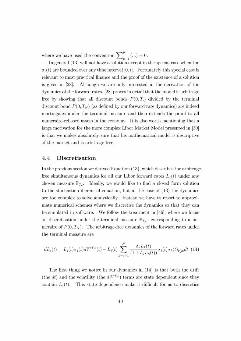
4.4 Discretisation
In the previous section we derived Equation (13), which describes the arbitrage-
free simultaneous dynamics for all our Libor forward rates Lj(t) under any
chosen measure PTp . Ideally, we would like to �nd a closed form solution
to the stochastic di¤erential equation, but in the case of (13) the dynamics
are too complex to solve analytically. Instead we have to resort to approxi-
mate numerical schemes where we discretise the dynamics so that they can
be simulated in software. We follow the treatment in [46], where we focus
on discretisation under the terminal measure PTN , corresponding to a nu-meraire of P (0; TN). The arbitrage-free dynamics of the forward rates under
the terminal measure are
dLj(t) = Lj(t)�j(t)dWTN (t)�Lj(t)
NXk=j+1
�kLk(t)
(1 + �kLk(t))�j(t)�k(t)�jkdt (14)
The �rst thing we notice in our dynamics in (14) is that both the drift
(the dt) and the volatility (the dW TN ) terms are state dependent since they
contain Lj(t). This state dependence make it di¢ cult for us to discretise
40

the dynamics accurately because we have to approximate the continuous drift
and volatility terms over discrete time intervals. We should like to remove
as much state dependence from our discretisation as possible.
Using the very useful structure of the Ito derivative of lnLj(t), we can
eliminate the state dependence of the volatility term by discretising lnLj(t)
rather than just Lj(t). Putting Xj(t) = lnLj(t), we have by Ito,
dXj(t) =1
Lj(t)dLj(t)�
1
2
1
Lj(t)2d hLj(t)i
=
"�
NXk=j+1
�kLk(t)�j(t)�k(t)�jk(1 + �kLk(t))
� 12k�j(t)k2
#dt+ �j(t)dW
TN (t)
Notice that the state dependence (the Lj(t) factor) has fallen out of the
volatility term but we are still left with a state dependent drift term.
To begin our discretisation we integrate both sides over our discretisation
timestep and apply a truncated Ito-Taylor expansion [37] to get
Xj(ti+1) = Xj(ti)+
ti+1Zti
"�
NXk=j+1
�kLk(u)�j(u)�k(u)�jk(1 + �kLk(u))
� 12k�j(u)k2
#du+
ti+1Zti
�j(u)dWTN (u)
We now approximate the stochastic terms Lk(u) over the time period
u 2 [ti; ti+1] with constants L�k to get
Xj(ti+1) ' Xj(ti) +
ti+1Zti
"�
NXk=j+1
�kL�k�j(u)�k(u)�jk(1 + �kL�k)
� 12k�j(u)k2
#du+
ti+1Zti
�j(u)dWTN (u)
= Xj(ti)�NX
k=j+1
�kL�k
(1 + �kL�k)�jk
ti+1Zti
�j(u)�k(u)du
�12
ti+1Zti
k�j(u)k2 du+ti+1Zti
�j(u)dWTN (u)
How do we choose these L�k? The simplest choice would be to use
41

L�k = Lk(ti), since we know this information at time ti. [32] states that most
banks use this approach and that, with a step size of about three months, the
error in the drift approximation is negligible. However [59] found that this
approximation is inaccurate for discretisations of three months or more (be-
tween two Libor reset dates) and recommends that the Predictor-Corrector
(PC) method be used. This method works as follows:
1. Initially, choose L�k = Lk(ti) to evolve X�j (ti+1) and hence L
�j(ti+1) =
exp(X�j (ti+1)).
2. Repeat the computation using L�k =12
�Lk(ti) + L�j(ti+1)
�to evolve
Xj(ti+1) and hence Lj(ti+1) = exp(Xj(ti+1)).
As can be seen from the PC algorithm, we are e¤ectively using the "av-
erage" Libor rates between times ti and ti+1 to determine the Libor rate
Lj(ti+1). It is not the true average because we have to estimate Lj(ti+1)
using L�j(ti+1) but [59] notes that this improved approximation of Lk(u) with
L�k yields very accurate results when compared to improving accuracy by
using much �ner discretisations.
So the discretised dynamics we implement are of the form,
Xj(ti+1) = Xj(ti)�1
2
ti+1Zti
k�j(u)k2 du+ti+1Zti
�j(u)dWTN (u)
�NX
k=j+1
�kL�k
(1 + �kL�k)�jk
ti+1Zti
�j(u)�k(u)du
Lj(ti+1) = eXj(ti+1)
(15)
When performing our discretisation we chose to apply a truncated Ito-
Taylor expansion to our stochastic di¤erential equation. This generally
obtains an order of strong convergence = 0:5 [37], which describes how the
error in discretisation diminishes with the decreasing size of the discretisation
mesh. It is possible to apply discretisation expansions that have better
42

orders of convergence: [37] recommends using the Milstein scheme as it is
hardly more complex than the simple Euler scheme and has an order of
strong convergence = 1. However [29] shows how we are already applying
the Milstein scheme to Lj(t) by our simulating its logarithm, Xj(t): little
advantage is realised applying the Milstein approximation to Xj(t).
Of more concern than the errors introduced by our discretisation is the
fact that our discretisation removes the martingale property from the dynam-
ics of Xj(t): the model is no longer arbitrage free [20]. Two adjustments
to the discretisation process are described in [20], where an adjustment is
made to the drift of Xj(t), and [43], where a completely di¤erent transform
of Lj(t) is discretised. Both describe how their improvements are marginal
under most conditions. We implement neither approach in this dissertation.
4.5 Pricing �nancial instruments
Equation (15) of the preceding section allows us to calculate Lj(t) at any time
t 2 Ti. The market data we have available are the initial term structure
Lj(T0) and the various modelled volatilities and correlations that allow us
to calculate the various integrals. These then allow us to build up an upper
triangular matrix of forward rates as shown in the left-hand matrix of Figure
7. Using (2) we can calculate the discount bonds P (Ti; Tj) in terms of these
forward rates as shown in the right-hand matrix of Figure 7.
Using these forward rates and discount bonds we should be able to model
the cash�ows of pretty much any interesting interest rate derivative. Section
6.4 explains what interest rate derivatives can be priced using the Libor Mar-
ket Model. We saw from Theorem 16 that if P (t; TN) is our numeraire and
PTN its corresponding equivalent measure, then the value of our derivativeV (t) is calculated by
V (t) = P (t; TN)(t)EPTN
�V (T )
P (TN ; TN)j Ft�
So to price a derivative for a particular set of evolved forward rates and
discount bonds at time t, we have to:
43

Figure 7: Examples of the matrices of forward rates and discount bonds thatare generated with each evolution of the forward rates. The rows correspondto measurements at particular points in time while the columns represent thefuture time periods at which the rates are relevant.
1. Calculate the cash�ows of the derivative at each time Ti.
2. Transport these cash�ows forward to time TN by dividing by our evolved
discount bonds P (Ti; TN).
3. Transport the combined TN payo¤s back to today (time t) by multi-
plying by today�s discount bond P (t; TN).
4.6 Hedging �nancial instruments: the Greeks
Section 4.5 describes how to use the Libor Market Model to calculate the price
of a �nancial instrument. This is the "fair" price of the instrument because
it is the same amount that theoretically can be realised in the market by
a synthetic instrument with identical payo¤s constructed using (dynamic)
hedging [42]. So it is important that once a trader has sold a �nancial
instrument (at a slight premium) she is able to lock in her pro�t by hedging
the instrument: she requires some recipe for her hedging activity. It is almost
certain that the ability to calculate a hedging strategy is more important than
the ability to calculate a price: often prices are visible in the market, but
it is the hedging strategy that allows the trader to mitigate risk and realise
pro�t. This section describes this hedging process.
Continuous-time arbitrage theory states that we need to be able to hedge
44

continuously to realise exactly the theoretical price of a �nancial instrument.
Hedging is achieved by shorting the delta of the instrument, making the com-
bined portfolio "delta-neutral". This means that the portfolio value should
remain almost constant over a small change in the value of the underlying
variables. Delta is calculated as the �rst derivative of the instrument price
with respect to its underlying variables. Delta is one of the "Greeks", a
collection of sensitivities of the option to various underlying variables that
are used for hedging purposes and risk management. In the case of the Libor
Market Model we have many underlying variables, the forward rates Li, so
we require a delta for each of them:
�i =@V
@Li
Obviously it is impossible to hedge continuously, and once liquidity re-
strictions and transaction costs are taken into account it might be impractical
to hedge more often than every few hours or days. This discrete delta-
hedging strategy is inaccurate and it is necessary to attempt to mitigate the
costs that are incurred by the less frequent hedging. To this end traders
also look at the gamma of the instrument and ensure that their portfolios
are both delta- and gamma-neutral. Gamma (another Greek) is calculated
as the second derivative of the instrument price (or the �rst derivative of
delta) with respect to its underlying variables. Notice that for each delta we
have one gamma for each underlying variable, so we have very many gammas
(equal to the square of the number of underlyings):
�ij =@2V
@Li@Lj
Among other reasons (as is discussed in Section 4.6.1), this explosive number
of gammas makes them di¢ cult to work with, and generally only the diagonal
gammas are calculated. In applications where the o¤-diagonal gammas
are required, they are referred to as cross-gammas. [18] brie�y discusses
how response surface techniques can be applied to approximate these cross-
gammas more e¢ ciently.
45

In addition to neutralising her portfolio against changes in the underly-
ing forward rates, the trader is generally also interested in the e¤ect that
changes in the market volatilities (vega is the Greek that measures sensi-
tivity to volatility) and correlations will have on the value of her portfolio.
By calculating sensitivities to these values the trader can attempt to hedge
against them. In the Libor Market Model we have to decide whether we wish
to calculate the sensitivities to the model volatilities (i.e. those of the for-
ward rates) or to the market implied volatilities (i.e. those of the caplets and
swaptions to which we calibrate). The �rst option, although computation-
ally straightforward, yields sensitivities to rather ephemeral measurements
of volatility: they are not readily visible in the market and so it is hard to
get a feel for them. The second option is extremely computationally expen-
sive because it requires recalibration of the Libor Market Model each time
a volatility is bumped. [51] and [53] present very lucid discussions of these
problems and the trade-o¤s involved.
Once we have the Greeks in terms of changes in the underlying forward
rates, we can quite easily calculate the Greeks in terms of discount bonds,
swaps and other market instruments used to build the yield curve by a simple
application of the chain rule [19].
In general, calculating the Greeks inside the Monte Carlo framework faces
several challenges: it can be slow and inaccurate compared to other pricing
techniques in the literature [18]. Additionally, Monte Carlo techniques are
normally required once a pricing problem becomes too complex for other
methods. When calculating the Greeks this complexity brings to the table
complications, like discontinuous payo¤s, where the Greeks are not smooth
or even extant! Although some progress has been made at improving the
performance of calculating the Greeks inside the Monte Carlo framework [19],
the complexity of the Libor Market Model renders most of these techniques
impractical.
There are two fundamental approaches to calculating the Greeks inside
the Monte Carlo framework:
� Finite di¤erence approximations. This is certainly the simpler of the
46
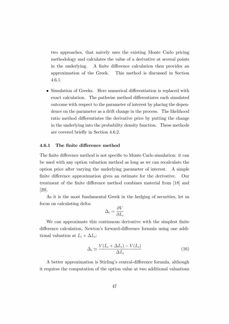
two approaches, that naively uses the existing Monte Carlo pricing
methodology and calculates the value of a derivative at several points
in the underlying. A �nite di¤erence calculation then provides an
approximation of the Greek. This method is discussed in Section
4.6.1.
� Simulation of Greeks. Here numerical di¤erentiation is replaced withexact calculation. The pathwise method di¤erentiates each simulated
outcome with respect to the parameter of interest by placing the depen-
dence on the parameter as a drift change in the process. The likelihood
ratio method di¤erentiates the derivative price by putting the change
in the underlying into the probability density function. These methods
are covered brie�y in Section 4.6.2.
4.6.1 The �nite di¤erence method
The �nite di¤erence method is not speci�c to Monte Carlo simulation: it can
be used with any option valuation method as long as we can recalculate the
option price after varying the underlying parameter of interest. A simple
�nite di¤erence approximation gives an estimate for the derivative. Our
treatment of the �nite di¤erence method combines material from [18] and
[29].
As it is the most fundamental Greek in the hedging of securities, let us
focus on calculating delta:
�i =@V
@Li
We can approximate this continuous derivative with the simplest �nite
di¤erence calculation, Newton�s forward-di¤erence formula using one addi-
tional valuation at Li +�Li:
�i 'V (Li +�Li)� V (Li)
�Li(16)
A better approximation is Stirling�s central-di¤erence formula, although
it requires the computation of the option value at two additional valuations
47

in the underlying at Li +�Li and Li ��Li:
�i 'V (Li +�Li)� V (Li ��Li)
2�Li(17)
Figure 8 provides a visual comparison of the two approximations. No-
tice how the central-di¤erence formula is superior to the forward-di¤erence
formula when approximating the tangent of a curve. Although it may seem
ine¢ cient to do twice as much work to calculate two additional points for
approximating delta using Stirling�s formula (17) its bias and variance proper-
ties are vastly superior to that of Newton�s formula (16) [18], and in addition
we can reutilise the same points when calculating the major gammas using
the approximation
�ii =@2V
@Li@Li
' V (Li +�Li)� 2V (Li) + V (Li ��Li)(�Li)
2 (18)
To determine how well our approximation of delta matches the actual
delta of the option we consider the bias and the variance of our approxima-
tion. The bias tells us to what error our approximation will converge, while
its variance tell us how quickly we will converge there. Let us �rst examine
the bias of our delta approximation:
biasi = E [�i]�@V
@Li
' E� �V (Li +�Li)� �V (Li ��Li)
2�Li
�� V 0(Li)
=1
2�LiE��V (Li +�Li)� �V (Li ��Li)
�� V 0(Li)
where �V is the average of the Monte Carlo simulations, and then Taylor
48

Figure 8: Comparison of Newton�s (dotted) and Stirling�s (dashed) approxi-mation to the actual (solid) gradient of the curve. Notice how much betterthe approximation is when using Stirling�s central di¤erence formula.
expanding our values around Li we get
biasi =1
2�LiE
" ��V (Li) + �L
0i�V (Li) +
12�L2
�V 00i (Li) +O(�L2i )
����V (Li)��L0i �V (Li) + 1
2�L2i �V
00(Li)�O(�L2i )� #� V 0(Li)
=1
2�LiE
"�V (Li) + �Li �V
0(Li) +12�L2i
�V 00(Li) +O(�L2i )
� �V (Li) + �Li �V 0(Li)� 12�L2i �V
00(Li) +O(�L2i )
#� V 0(Li)
=1
2�LiE�2�Li �V
0(Li) +O(�L2i )�� V 0(Li)
=1
2�LiE�O(�L2i )
�= O(�Li)
So we see that we can arbitrarily reduce the bias of our estimate by
reducing �Li, although we must remain aware of machine precision issues
49

[7]. Let us now consider the variance of our delta approximation:
variancei = V ar [�i]
' V ar
� �V (Li +�Li)� �V (Li ��Li)2�Li
�=
1
4�L2iV ar
��V (Li +�Li)� �V (Li ��Li)
�=
1
4�L2inV ar [Vn(Li +�Li)� Vn(Li ��Li)]
The last step assumes that the Vn, which comprise the average �V are i.i.d
as is argued in [18]. The 14�L2i
term suggests that variance might become
explosive as we reduce �Li unless the variance term contains a �Li or �L2iterm in the numerator to compensate for the�L2i in the leading denominator.
[18] gives three scenarios for the order of V ar [V (Li +�Li)� V (Li ��Li)]:
� O(1) : If Vn(Li+�Li) and Vn(Li��Li) are computed independently.
� O(�Li) : If Vn(Li+�Li) and Vn(Li��Li) are computed using commonrandom numbers.
� O(�L2i ) : If Vn(Li+�Li) and Vn(Li��Li) are computed using commonrandom numbers and that Vn is su¢ ciently smooth in Li.
Clearly the third scenario would be optimal, but we can only guarantee
the second scenario, where we use the same random numbers when calcu-
lating the value of our option at the di¤erent points of the �nite di¤erence
approximation. In this case our variance is:
variancei =1
4�L2inO(�Li)
= O
�1
�Li
�So although we can improve our bias arbitrarily by decreasing �Li, the
variance of our measurement simultaneously grows as we decrease �Li. So
we have to trade-o¤ between reducing bias and increasing variance. [49]
50
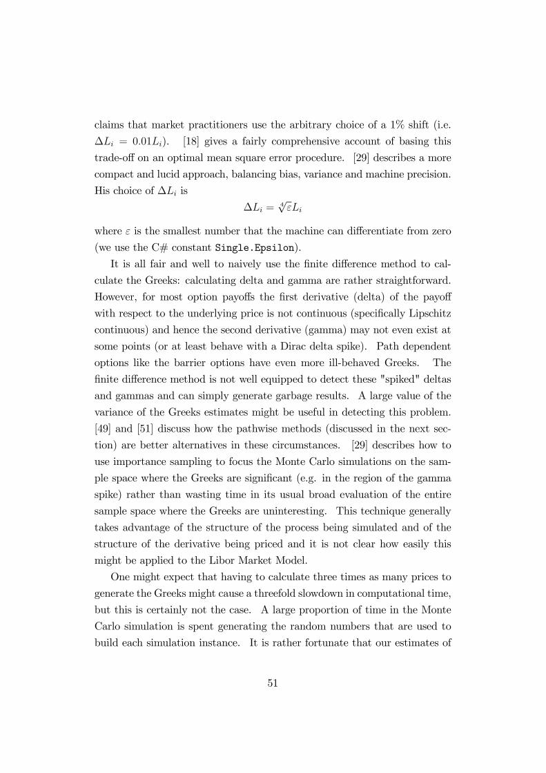
claims that market practitioners use the arbitrary choice of a 1% shift (i.e.
�Li = 0:01Li). [18] gives a fairly comprehensive account of basing this
trade-o¤ on an optimal mean square error procedure. [29] describes a more
compact and lucid approach, balancing bias, variance and machine precision.
His choice of �Li is
�Li =4p"Li
where " is the smallest number that the machine can di¤erentiate from zero
(we use the C# constant Single.Epsilon).
It is all fair and well to naively use the �nite di¤erence method to cal-
culate the Greeks: calculating delta and gamma are rather straightforward.
However, for most option payo¤s the �rst derivative (delta) of the payo¤
with respect to the underlying price is not continuous (speci�cally Lipschitz
continuous) and hence the second derivative (gamma) may not even exist at
some points (or at least behave with a Dirac delta spike). Path dependent
options like the barrier options have even more ill-behaved Greeks. The
�nite di¤erence method is not well equipped to detect these "spiked" deltas
and gammas and can simply generate garbage results. A large value of the
variance of the Greeks estimates might be useful in detecting this problem.
[49] and [51] discuss how the pathwise methods (discussed in the next sec-
tion) are better alternatives in these circumstances. [29] describes how to
use importance sampling to focus the Monte Carlo simulations on the sam-
ple space where the Greeks are signi�cant (e.g. in the region of the gamma
spike) rather than wasting time in its usual broad evaluation of the entire
sample space where the Greeks are uninteresting. This technique generally
takes advantage of the structure of the process being simulated and of the
structure of the derivative being priced and it is not clear how easily this
might be applied to the Libor Market Model.
One might expect that having to calculate three times as many prices to
generate the Greeks might cause a threefold slowdown in computational time,
but this is certainly not the case. A large proportion of time in the Monte
Carlo simulation is spent generating the random numbers that are used to
build each simulation instance. It is rather fortunate that our estimates of
51
the Greeks are better when we reuse these random numbers. Experimentally
we found that the computation of delta and gamma for each forward rate
takes only around an additional 30% of the time it takes to price the option
itself.
4.6.2 Other approaches: the pathwise method and the likelihoodratio method
Not implemented for this dissertation, but worth describing brie�y are two
other methods exist for estimating the Greeks of various derivative products.
They attempt to produce unbiased estimates by replacing numerical di¤er-
entiation with exact calculations. The pathwise method di¤erentiates each
simulated outcome with respect to the parameter of interest by placing the
dependence on the parameter as a drift change in the process; the likelihood
ratio method di¤erentiates by putting the dependence in the probability den-
sity function. The two methods are covered in detail in [12]. The pathwise
method seems to be the more stable of the two approaches [51] and is ap-
preciably faster to calculate than the �nite di¤erence method [49]. Its only
drawback is that it requires continuous derivative payo¤s. The likelihood
ratio method works well with options with discontinuous payo¤s but can
generate unstable estimations for the Greeks. Neither method is as gen-
eral as the �nite di¤erence method, which can be applied to any derivative
product. Both the pathwise method and the likelihood ratio method require
some mathematics to be performed on the payo¤ of each derivative being
priced.
52

5 Model details
The Libor Market Model requires several inputs: today�s forward rates, for-
ward volatilities and correlations between forward rates. These three sources
of information can not simply be looked up on a market data terminal. They
are instead derived using somewhat complex procedures from instruments
traded in the market. Forward rates are bootstrapped from deposit rates,
bonds and swaps; forward rate volatilities are estimated from caplet volatili-
ties, which are in turn bootstrapped from traded caps; forward rate correla-
tions can be inferred from swaption volatilities. All these choices of market
data, bootstrap procedures and inference algorithms can yield vastly di¤er-
ent input parameters for the Libor Market Model, and understandably can
lead to hugely varying estimates for modelled derivative prices. Indeed [60]
presents a study on how many di¤erent prices one can arrive at for the same
option using di¤erent calibrations that are consistent with market data. [59]
and [60] describe how successful application of the Libor Market Model lies
somewhere between science and an art. This unfortunate state of a¤airs is
summed up by [65], who states that all models he has ever seen are demon-
strably wrong, but in experienced hands they are powerful pricing tools.
This section describes how the information in the market is intelligently
translated into a form that is acceptable and reasonable as inputs to the
Libor Market Model.
5.1 The initial forward rates
Forward rates lie at the heart of the Libor Market Model and are generally
implied from the market yield curve. This yield curve is built up using
a variety of techniques from the deposit rates, bond prices and swap rates
that are available in the market. There are a plethora of techniques in the
literature on how to bootstrap this yield curve, each with its advantages and
disadvantages: [22] presents many of them in detail. On top of the choice of
bootstrap methodologies to use, the implementor must choose between the
"grade" of interest rate product that is used in the bootstrap. Government
bonds yield lower returns than riskier corporate bonds; swaps between A-
53
grade counterparties carry di¤erent rates to those between less credit-worthy
customers; overnight Libor rates are available only to the larger banks. Also,
[59] explains how each investment bank might have its own views on the
future realisations of the yield curve and so when pricing, a trader might
not want to use the equilibrium rates in the market caused by supply and
demand, but rather might wish to incorporate her own subjective view of the
future forward rates.
Once the forward rates prevailing today have been established we can
move on to describing the dynamics of the forward rates, �rst as solitary en-
tities (by looking at their volatilities, see Section 5.2), and then as a group of
entities that in�uence each others�behaviour (by looking at their correlation,
see Section 5.3).
5.2 Volatility speci�cation
Probably the most important parameters of the Libor Market Model are
the volatilities of the forward rates. They play a role not only in the sto-
chastic part of the evolution of our forward rates, but more importantly in
the deterministic drift adjustments that each rate enjoys under the terminal
measure. Inside the model, the speci�cation of the instantaneous volatility
�i(t) for each forward rate Li(t) is pretty �exible, with the only pressing req-
uisites being that it be deterministic and integrable (the Novikov condition
of Lemma 9).
This in�nite-dimensional (over continuous time) instantaneous volatility
parameter allows us great �exibility in calibrating the forward rate volatilities
to those found in the market. When deciding how we want to specify our
forward volatilities we have to be careful that we do not give our model so
much �exibility that it is easily allowed to become over-calibrated. An over-
calibrated model generally performs poorly at modeling the future because
it has learned the temporal (and even noisy) characteristics of the present
market rather than the general time-invariant characteristics of the present
market that might model the future market e¤ectively.
The primary means of calibrating the volatilities of the forward rates
54

Figure 9: Hypothetical caplet market data
in the Libor Market Model is using the caplet implied volatilities that are
quoted in the market. We will see how this is done in Section 5.4. For
now let us focus on what information is actually provided by the market and
determine a parsimonious speci�cation for the volatility of our forward rates
that might capture the essence of the volatilities of the forward rates. Figure
9 show some hypothetical caplet data that is available in the market.
We are given three caplets capleti with expiries Ti�1, i = 2 : : : 4, each
with their own underlying forward rate Li with implied Black76 volatility �i.
There is no initial caplet caplet1 because by de�nition it is a caplet on the
forward rate L1 which is the (forward) rate from time T0 to time T1, which
is known at T0. Now the Black76 volatility �i is just the "average squared
volatility over time" of the underlying forward rate Li, i.e.
�2i =1
Ti�1 � T0
Z Ti�1
T0
�2i (u)du
The simplest speci�cation might set �2i (u) to the constant �2i , but this
leads to an instantaneous volatility speci�cation that is not time-homogeneous
55

[59]. This means that at some snapshot of the future, our model will describe
forward rate volatilities di¤erently than today. We have no reason to expect
a forward rate today with one week to expiry to have signi�cantly di¤erent
behaviour to a forward rate in a year�s time with one week to expiry. A
time-homogeneous model will ensure that behaviour modelled today is the
same as behaviour modelled in the future. Another problem with the con-
stant speci�cation is that it does not take into account the humped shape of
the term structure of instantaneous volatility that is visible in the market:
for long-dated caplets, a large portion of the total volatility of caplets seems
to be derived in the period from six-months to two-years of its inception [57].
One method of ensuring that our speci�cation is time-homogeneous is to
parametrise it solely on the remaining time to expiry of the caplet, i.e.
�i(t) = f (Ti�1 � t)
where Ti�1 is the expiry of the caplet, t is the point where we are measuring
the instantaneous volatility of the underlying forward rate and f is some
function.
After analysing numerous sets of market data, [57] suggests the speci�-
cation of
�i(t) = [a+ b (Ti�1 � t)] e�c(Ti�1�t) + d (19)
which he argues is suitable because
� it is time-homogeneous;
� it has a �exible form able to reproduce humped or monotonically de-
creasing instantaneous volatilities that pervade the market;
� its parameters have relatively transparent economic interpretation; and
� it has an e¢ cient analytical representation of the square integralR�i(u)�j(u)du,
which is required during calibration and evaluation of the covariances
during simulation
An example of the term structure of volatilities produced by (19) is shown
in Figure 10. [59] provides lucid descriptions of the characteristic shape of
56

Figure 10: An example of the term structure of volatilities. Notice thecharacteristic "hump" around the one- to two-year period.
the market instantaneous volatilities and of the economic interpretation of
the speci�cation parameters.
The determination of the four parameters a; b; c; d are covered in Section
5.4. For completeness (and for practicality�s sake), I include not the mathe-
matical representation of the square-integral of (19), but rather the C# code
for it in Section 10.1. The code was translated from the c++ code available
at [43].
Although (19) provides a time-homogenous description of the volatility of
the market, it is not likely to exactly �t all the market data simultaneously.
When pricing certain derivatives, especially products similar to caplets (e.g.
barrier caplets), it is important that the model correctly calculates the cur-
rent market price of the caplets used for calibration. [59] suggests adding a
touch of inhomogeneity to the speci�cation by writing it in the form
�i(t) = Ki
�[a+ b (Ti�1 � t)] e�c(Ti�1�t) + d
�where Ki is a scaling constant that allows complete calibration to the market
57

data. Generally speaking, if (19) provides a reasonable �t to the market data
these Ki should be very close to unity, and thus the level of time-inhomogeity
introduced is minimal. The addition of this constant does not substantially
alter the complexity of the square-integral: it merely introduces the factor
KiKj in front of the integral.
5.3 Correlation speci�cation
Having speci�ed the instantaneous volatilities of the forward rates in our
model we are half way to completely describing their dynamics. What re-
mains is the speci�cation of the correlation, and thus covariance, between
the various forward rates. The covariance between the forward rates ap-
pears in the deterministic drift adjustments that each rate enjoys under the
terminal measure, and has a particularly large impact of correlation sensitive
instruments such as long-dated Bermudan swaptions [59].
We are faced with two problems when specifying our forward rate corre-
lation matrix:
� Correlations are not directly visible in the market. They have either
to be approximately derived from swaption prices (covered in Section
5.5), estimated by an experienced market participant or calculated from
historical data. [1] describes how calibration to historical data leads to
calibration that is not at all time-homogenous and is rather unstable
over time.
� Being able to specify a large number of correlation coe¢ cients may yieldan over-calibrated model that may not model the future very well.
Correlations between forward rates can become quickly unmanageable:
given n forward rates, there are n(n�1)2
distinct correlation coe¢ cients be-
tween them. For example, a long dated Bermudan swaption spanning 20
years with six-monthly cash�ows spans 40 forward rates and 780 correlation
coe¢ cients! Rather than calibrate each individual correlation coe¢ cient, we
therefore seek a parsimonious speci�cation for the forward rate correlations
that adequately describes what scant information is available in the market.
58

Such speci�cations are the topic of active research [11], [8], [14], [15], [43],
[59]. The model we choose is one described in [59]. It has the form:
�ij = �+ (1� �) e��jTi�Tj j (20)
where � is a long term minimum correlation between two forward rates and
� describes the sensitivity of the correlation between two forward rates to the
di¤erence between their expiries. [32] recommends the parameters � = � =
0:1 as being re�ective of the UK market. Under this model two forward rates
with nearby expiries (e.g. 1-year and 2-year) will have a high correlation,
while two forward rates with greatly di¤erent expiries (e.g. 1-year and 10-
year) will have a low correlation. This seems in keeping with the market
[59]. Some authors argue that the correlation between the 1- and 2-year
forward rates should be lower than that of the 19- and 20-year forward rates
[8] because market participants have more strongly con�icting views about
the short end of the yield curve than the long end, but [31] and [59] defend it.
An example of the correlation matrix produced by (20) is shown in Figure
11, where the �oor axes are the expiries of each of the underlying forward
rates and the vertical axis is the correlation between them.
We have chosen this correlation speci�cation because of its concise formu-
lation and because its �nancial implications can be readily explained. The
downside of our choice is that this speci�cation leads to a multi-factor Libor
Market Model that has as many factors as there are forward rates. Section
5.6 describes why this might be unreasonable and shows how we can reduce
this number of factors. Alternative speci�cations are presented in [8], [14]
and [59] where correlation matrices are produced that implicitly have a small
number of factors, but they lose the intuitive relation of their speci�cations
to �nancial reality.
5.4 Calibration to caplets
We begin the calibration of our Libor Market Model to the market by en-
suring that it correctly prices a set of caplets available in the market. We
showed in Section 3.4.1 how the market arrives at the Black76 implied volatil-
59

Figure 11: An example of the parametrisation of the correlation betweenforward rates. The �oor axes represent the year of expiry of the forwardrates and the vertical axis their correlation.
ity for a caplet. Ideally we would like to �nd in the market a set of caplets
that span the time periods over which we wish to price more complex deriv-
atives using our model. One generally will not go to the market to �nd the
market prices for the various caplets as these prices are likely to be biased
(the spread and skews that the traders add to customer facing prices) or stale
(if they are illiquid and seldom traded). Generally speaking, these implied
market volatilities will be provided in-house by the interest rate traders [10],
probably stripped from their cap prices combined with personal adjustments
applied to cap volatilities. [9] describes how to perform this stripping.
Having collected the implied (Black76) volatilities ��i for N spanning
caplets expiring at Ti�1 and paying out at Ti, our task is simply to �nd
the combination of parameters a; b; c; d of Equation (19) that minimises the
objective function
error =NXi=1
0@��2iTi�1 �Ti�1Z0
�2i (u; a; b; c; d) du
1A2
60

The location of the optimal parameters requires an iterative global opti-
misation method, several of which are described in [54]. We use the Nelder-
Mead global search algorithm that is described in Section 6.3.
Once we have discovered the optimal set of parameters a; b; c; d we have
calibrated the continuous speci�cation for the instantaneous volatility such
that
��2iTi�1 'Ti�1Z0
�2i (u; a; b; c; d) du
Note that it is unlikely that we will have exact parametrisations for the
market volatilities so we de�ne Ki such that
��2iTi�1 = K2i
Ti�1Z0
�2i (u; a; b; c; d) du
i.e.
Ki =
vuuuuut��2iTi�1
Ti�1Z0
�2i (u; a; b; c; d) du
(21)
Section 7.1 shows the results of our calibrating to caplets using this tech-
nique.
5.5 Calibration to caplets and swaptions
The previous section showed how to calibrate the Libor Market Model to the
implied volatilities of caplets in the market. That calibration ensures that
our model correctly prices the caplets. This should then ensure that the
prices of more complex derivatives are realistic - especially those that have
very similar characteristics to caplets. Unfortunately there are many impor-
tant interest rate derivative products that rely on not only the instantaneous
volatility of the underlying forward rates but also (and generally more im-
portantly) on the correlations between them. The instrument of this form
that has received the most attention is the Bermudan swaption [2], [36] and
61

[59].
One might expect that the various swap market models (in contrast to
the Libor Market Model) might be better suited to modelling derivatives
that exhibit features that are more similar to swaptions than to forward rate
derivatives, but [59] argues that the Libor Market Model is a better modelling
framework for reasons of simplicity, understandability and e¢ ciency. In
addition, being able to calibrate the Libor Market Model simultaneously
to caplets and swaptions allows us to automatically price derivatives that
employ features from both markets.
As was seen in Section 5.3, our speci�cation of the correlation between the
forward rates was simply a time-homogenous speci�cation that was monoton-
ically decreasing on the absolute di¤erence between forward rate expiries.
Other than the broad market calibration of the parameters � and �; no at-
tempt was made to capture any more information that might be available in
the market. This section motivates an approach that ensures that at least
the market price of swaptions is correctly determined by our Libor Market
Model because a large number of derivative products behave quite similarly
to these swaptions. We showed in Section 3.4.2 how the market arrives at
the Black76 implied volatility for a swaption.
Now any attempt to jointly calibrate to the market prices of caplets and
swaptions assumes that their prices are mutually consistent. Both [40] and
[57] describe where this assumption is sometimes violated. Generally speak-
ing, swaptions are priced higher than they should be because the market
requirement for them is very one-sided (everyone is buying), so we rely heav-
ily on the information provided by the market caplet prices and adjust only
slightly to the information provided by the market swaption prices.
We combine the methodologies presented in [33], [35], [58] and [32].
From (3) we have the swap rate
SRi =NXj=i
wi;jLj
=) dSR i =NXj=i
(dwi;jLj + wi;jdLj + dwi;jdLj)
62

[59] gives the compelling argument that wi;j remains pretty much constant
for �rst-order (roughly parallel shifts) and second-order (more complex shape
changes) changes to the yield curve and that these changes are most prevalent
in practice. If we make the assumption that wi;j is constant then the dwi;jterms fall away, leaving
dSRi =
NXj=i
wi;jdLj
So we know we can write our swap rates in terms of our forward rates.
Now a fundamental assumption of the Libor Market Model is that the for-
ward rates have lognormal dynamics. [30] and [56] show that if we assume
lognormal dynamics for the forward rates then the dynamics of the swap
rates can not be lognormal. Indeed not only are the swap rate dynamics not
lognormal, but their drift and volatility terms are stochastic [56]. To pro-
ceed with our calibration to swaptions we make the simplifying assumption
that the swap rates have lognormal dynamics. [34] and more recently [35]
describe how accurate this assumption is in practice.
If we assume the forward rates and swap rates have lognormal dynamics,
then we can attempt to write the swap rate volatilities in terms of the forward
rate volatilities. Focussing only on the volatility terms we can write the
dynamics for lnSRi under the terminal measure PTN :
dSRi = �SRi SRidWTN + (� � � )SRidt
dSRi
SRi
= �SRi dW TN + (� � � ) dt
d lnSRi = �SRi dW TN + (� � � ) dt
We can write the equivalent expression for the dynamics of lnSRi in
63

terms of forward rates as,
d lnSRi =NXj=i
@ lnSRi
@ lnLjd lnLj + (� � � ) dt
'NXj=i
@ lnSRi
@ lnLjd lnLj
=NXj=i
LjSRi
@SRi
@Ljd lnLj
=
NXj=i
Zid lnLj
where
Zij =LjSRi
@SRi
@Lj
' LjSRi
� wi;j (22)
and
wi;j =�jP (Tj)NXk=i
�kP (Tk)
(23)
We wish to determine the relationship between the covariance matrices
of swap rates and the Libor forward rates, so
E [d lnSRid lnSRj] = E
"NXm=i
Zimd lnLm
NXn=j
Zjnd lnLn
#
= E
"NXm=i
NXn=j
Zimd lnLmd lnLnZ0
nj
#=) CSR = ZCLZ
0
where CSR and CL are the covariance matrices for the swap rates and the
Libor forward rates, respectively.
If we consider (22) we see that Zij is upper triangular: Zij = 0 for j < i
64

(since the swap rate does not depend on the forward rates before its initial
cash�ow) and Zij 6= 0 for i = j (since the swap rate is certainly dependent
on the forward rate of its reset date). Thus Z is invertible and we can move
freely between the two covariance matrices using
CSR = ZCLZ0
(24)
CL = Z�1CSR�Z0��1
(25)
Note that the speci�cation of Z by (22) is a continuous time speci�cation.
More interestingly, it is stochastic because it contains Lj. This means that
the covariance matrix for our swap rates is also stochastic. To avoid the
theoretical complexity of stochastic covariances and the computational com-
plexity of calculating Z at each timestep we make the further approximation
of using the T = 0 value of Z throughout the evolution of our forward rates
and swap rates. [35] gives evidence that this approximation is reasonable
and describes its (occasional) shortcomings. Thus we use
CSR(0; Tj) = Z(0)CL(0; Tj)Z0(0)
We are now in a position to calibrate to the market swaption prices. If
�j is the market implied volatility of swaption j, then it should be equal to
�j =
s1
TjCSRjj (0; Tj)
It is unlikely that the market volatility �j matches our model volatility
�j, so we set
�j =�j�j
and
� =
2664�1 0 0
0. . . 0
0 0 �n
3775
65

Our swaption calibrated Libor covariance matrix CL is then
CL(0; Tj) = Z(0)�1�Z(0)CLZ(0)0��Z(0)
0��1
Although this method works well for most yield curves, both [32] and [33]
suggest improvements in the approximation of the wi;j for very steep yield
curves. Note that this method of calibration to swaption volatilities makes
no mention of the covariance between the swap rates. The correlations
between the swap rates and the forward rates are determined only by the
correlations between the forward rates, with a little in�uence creeping in from
the calibrated swaption volatilities. [32] notes that this is not completely
unnatural: coterminal swap price covariances are not something that are
readily visible in the market.
The method of calibrating to swaption volatilities used in this dissertation
is by no means the only approach covered in the literature: [14], [15] and [59]
present other approaches that they feel have more compelling justi�cation.
5.6 Factor reduction
As was explained in Sections 4.2 and 5.3, we have implemented a multi-factor
Libor Market Model. That means that our forward rates react in di¤erent
ways to several sources of noise through their sensitivity (expressed via their
volatilities �j(t)) to each dimension of the Brownian motion dW Tj(t). [32]
shows how several factors are indeed necessary to adequately capture the re-
lationship between the various forward rates and correctly price derivatives
such as Bermudan swaptions that are highly dependent on the correlation
structure between the forward rates. That said, the model we have imple-
mented so far has as many factors as there are forward rates and [32] notes
that there is no noticeable improvement to pricing using more than three or
four factors. We really are performing unnecessary work and this can slow
down computation almost linearly in the number of factors because we have
to generate a random number for each of the factors and update the forward
rates according to their sensitivities to each factor.
66

This section describes a method of reducing the number of factors rep-
resented by our correlation matrix by picking out the "most important fea-
tures" of the correlation speci�cation. There are many approaches in the
literature to deciding exactly what we mean by the "most important fea-
tures" [21], [32] and [59]. We implement the method in [32] that builds a
correlation matrix by retaining only the eigenvectors corresponding to the
largest eigenvalues of the original correlation matrix.
Assume that we have a correlation matrix C of the form described in
Section 5.3. We �nd the N eigenvalues �i and corresponding eigenvectors eiof matrix C: our correlation matrices are real and symmetric and so can be
quickly reduced to Householder form and the eigensystem e¢ ciently solved
using the QL algorithm [54]. The matrix R with N columnsp�iei is a
pseudo-square root of C. Let R(M) be the matrix whose �rst M columns
are thep�iei corresponding to the largest (in absolute value) eigenvalues
�i and remaining N �M columns set to zero. Then R(M) is the M -factor
pseudo-square root of C, and ~C(M) = R(M)�R(M)
�Tis a matrix with only
M factors. Note that ~C(M) will not be a correlation matrix because the
diagonal elements are not likely to be unity. It will, however, be symmetric
and so we can turn it into the correlation matrix C(M) by setting
C(M)ij =
~C(M)ijq
~C(M)ii
~C(M)jj
C(M) is then the M -factor correlation matrix we use in our Monte Carlo
simulations exactly as we would have used C before. We will see the e¤ect
that factor reduction has on option prices in Section 7.4.
67

6 Technical details
6.1 Monte Carlo integration
Ideally, we would like to be able to solve the forward rate dynamics (13)
analytically so that we might have a closed form solution Lj(t) at any time
t 2 [0; TN ]. Unfortunately (13) is far too complex to solve analytically, andthe problem becomes worse when we wish to calculate the expected value of
derivatives with optionality, as we then need also to know the distribution of
the Lj(t).
To this end we have to turn to numerical methods to calculate our deriv-
ative prices. These numerical methods include the various tree techniques,
�nite di¤erence PDE methods and Monte Carlo technique [66]. The tree
techniques and �nite di¤erence PDE methods work well for problems with
low dimensionality, but once the number of dimensions becomes too large
their computation time becomes unreasonable - the so-called curse of dimen-
sionality [66]. The method of choice for solving problems with complicated
dynamics and high-dimensionality is the Monte Carlo technique [18].
Let us examine the mathematics of the Monte Carlo technique. We
should like to examine how our Monte Carlo approximations converge to the
actual solution. The mathematics is covered in more detail in [29].
We use Monte Carlo simulations in �nance to calculate the expectation
of various derivative payo¤s f(x), under generally complex distributions of
underlying processes (x), over some domain D.
V = E (x) [f(x)]
=
Zx2D
f(x) (x)dx
The Monte Carlo approximation to the above expectation is simply
VN =1
N
NXi=1
f(xi) where xi � (x)
If the sequence of random variates f(xi) has mean � and variance �2,
68

then the Central Limit Theorem [29] tells us that
VN �! N��;
�pN
�Although we do not know the variance of f(xi) we can combine the Cen-
tral Limit Theorem and the Continuous Mapping Theorem [29] to use the
variance of our Monte Carlo simulation as an estimate for �2:
�N =
vuut 1N
NXi=1
f(xi)2
!� 1
N
NXi=1
f(xi)
!2
We de�ne the standard error �N as
�N =�NpN
Note that the standard error does not provide a guaranteed range inside
which the true answer lies; it is a statistical measure. This means that there
is a chance that the simulation answer lies outside the range of the standard
error. We use the standard error to help determine when to stop the simula-
tion and some give some indication of the error of the result. But it is up to
the user of the model to decide on the convergence of the simulation, gener-
ally by inspecting the "average-so-far" as the simulation progresses. Figure
12 shows an example of the convergence of the Monte Carlo simulation. No-
tice how the price starts o¤ erratically but after several thousand iterations
converges towards a solution. Also note the inverse square-root behaviour
of the standard error: it becomes increasingly di¢ cult to further reduce the
standard error as the number of iterations increases.
There exists a vast literature on the various techniques that can be applied
to increase the convergence speed of the Monte Carlo method. [7] covers
these in some detail. We will make explicit use only of antithetic variables
in Section 6.2.3 and implicit use of moment matching with Sobol sequences
in Section 6.2.2. Control variates are a powerful mechanism for reducing
simulation variance but are generally speci�c to the product being priced,
69

Figure 12: An example of a Monte Carlo simulation. Notice that the priceconverges towards a solution as the standard error drops with the inversesquare-root of the number of iterations.
and so are not covered in this dissertation.
6.2 Random numbers
This section describes the various mechanisms we have at our disposal for gen-
erating the "random" numbers for the Brownian factors in our Monte Carlo
simulations. Excluding custom-built hardware for generating truly random
numbers, there is no such thing as a computer-generated random number:
the computer has to follow an algorithm to generate these sequences, and any
algorithm is deterministic and can be repeated. We cover the generation of
two broad categories of random numbers: pseudo- and quasi-random. The
former attempts to mimic truly random numbers by using interesting prop-
erties of mathematical constructs and is presented in Section 6.2.1; the latter
attempts to cover a domain as comprehensively as possible while maintain-
ing the same distribution as a random number and is presented in Section
6.2.2. Section 6.2.3 then explains how a pseudo-random source can be made
70

to better cover a domain through the use of antithetic variables. Finally,
Section 6.2.4 discusses how uniformly distributed numbers are converted to
numbers from the Gaussian distribution: we need Gaussian draws to simulate
Brownian motion.
6.2.1 Pseudo-random numbers
Pseudo-random numbers are produced by deterministic algorithms to form
sequences that attempt to imitate the distribution of truly random numbers.
As was said before, there is no such thing as a computer-generated truly
random number. Instead the inventors of the random number generators
rely on the ingenious manipulation of mathematical properties of numbers to
extract numbers that appear random. Although most computer languages
come with libraries for generating uniformly distributed pseudo-random num-
bers, both [7] and [54] give compelling reasons for why we should implement
a robust pseudo-random number source for Monte Carlo simulation. The
most compelling is probably that some platform provide random number
generators that are hardly acceptable at all: they may produce numbers
that are not uniformly distributed; sequences that repeat after only sev-
eral thousand draws; or sequences that exhibit undesirable patterns in high
dimensions. Another useful reason is that if the pseudo-random number
generator is speci�ed, we can be sure that we will generate exactly the same
sequence of numbers across two Monte Carlo runs if we wish to. This can be
helpful for debugging and calculating prices and the Greeks in a distributed
computing environment, where multiple computers might need to use the
same set of random numbers.
We implement the Mersenne Twister algorithm as presented in [41]. [29]
describes it as being the best available, both in terms of speed and in terms of
satisfying the properties we would like from a Monte Carlo random number
source. The code for the algorithm is presented in Section 10.4.
71

6.2.2 Quasi-random numbers
Although the Mersenne Twister random numbers discussed in the previ-
ous section provide a reliable source of uniformly distributed pseudo-random
numbers, it has been found that for Monte Carlo integration techniques, bet-
ter results are achieved using uniformly distributed quasi-random numbers
that better cover the region of integration [7]. Two of the most established
sources of these quasi-random numbers are the Niederreiter [47] and Sobol
[61] sequences. [29] argues that the Sobol sequences are better than Nieder-
reiter sequences for high-dimensional problems as long as they have been
correctly initialised. [49] also gives recommendations of how the Brownian
bridge should be used with high-dimensional Sobol sequences to avoid any
problems with the higher dimension sequences becoming coplanar.
The next section describes the implementation of antithetic variables.
By their nature, Sobol sequences have a degree of implicit antithetics (and
moment matching for that matter) as long as you take care to run your Monte
Carlo simulation with a number of iterations that is a power of 2.
Note that if computation speed is important in pricing many di¤erent
derivatives in a portfolio, both the pseudo-random and quasi-random num-
bers can be precalculated and used again and again.
6.2.3 Antithetics
The variance of a Monte Carlo simulation can be reduced by producing neg-
ative correlations between the numerous paths generated during the simula-
tion. The simplest approach to producing these negatively correlated paths
is the method of antithetic variables. It relies on the fact that if random
variable U is uniformly distributed then so is U = 1�U . This translates toGaussian draws using the technique in section 6.2.4 that have the same mag-
nitude but opposite signs, i.e. Z � F�1(U) = �F�1(U) � �Z, where F�1 isthe inverse transform of the Gaussian distribution. This in turn translates
to antithetic sequences of random draws (Z1; : : : ZN) and (Z1; : : : ZN) that
produce antithetic simulations of the Libor rate using equation 15.
These antithetic simulations of the Libor rate, L and L should be nega-
72
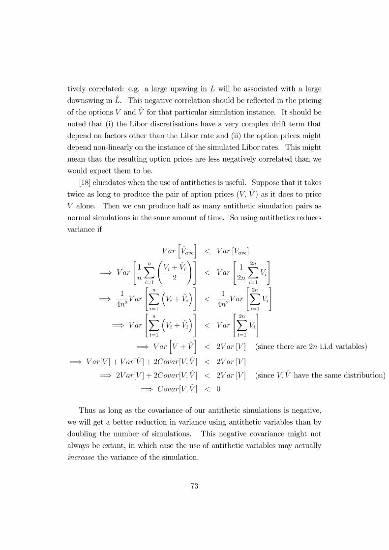
tively correlated: e.g. a large upswing in L will be associated with a large
downswing in L. This negative correlation should be re�ected in the pricing
of the options V and V for that particular simulation instance. It should be
noted that (i) the Libor discretisations have a very complex drift term that
depend on factors other than the Libor rate and (ii) the option prices might
depend non-linearly on the instance of the simulated Libor rates. This might
mean that the resulting option prices are less negatively correlated than we
would expect them to be.
[18] elucidates when the use of antithetics is useful. Suppose that it takes
twice as long to produce the pair of option prices (V; V ) as it does to price
V alone. Then we can produce half as many antithetic simulation pairs as
normal simulations in the same amount of time. So using antithetics reduces
variance if
V arhVave
i< V ar [Vave]
=) V ar
"1
n
nXi=1
Vi + Vi2
!#< V ar
"1
2n
2nXi=1
Vi
#
=) 1
4n2V ar
"nXi=1
�Vi + Vi
�#<
1
4n2V ar
"2nXi=1
Vi
#
=) V ar
"nXi=1
�Vi + Vi
�#< V ar
"2nXi=1
Vi
#=) V ar
hV + V
i< 2V ar [V ] (since there are 2n i.i.d variables)
=) V ar[V ] + V ar[V ] + 2Covar[V; V ] < 2V ar [V ]
=) 2V ar[V ] + 2Covar[V; V ] < 2V ar [V ] (since V; V have the same distribution)
=) Covar[V; V ] < 0
Thus as long as the covariance of our antithetic simulations is negative,
we will get a better reduction in variance using antithetic variables than by
doubling the number of simulations. This negative covariance might not
always be extant, in which case the use of antithetic variables may actually
increase the variance of the simulation.
73

Figure 13: Examples of the various random number sources. From leftto right: Sobol sequence; Mersenne Twister; and Mersenne Twister withantithetic variables.
As mentioned in the previous section, Sobol sequences automatically in-
cludes the concept of antithetic variables.
6.2.4 Gaussian draws
[64] discusses the care that should be taken when generating random numbers
from the Normal distribution using uniform draws, especially when it comes
to the translation of points near the extremes of the distributions. We
have selected Moro�s algorithm for transforming the "uniformly distributed"
numbers between 0 and 1 (generated using the Mersenne Twister or via Sobol
sequences) into Normally distributed numbers as it is reportedly accurate to
15 decimal places, even out in the tails of the distribution! I should like to
thank Dr. Graeme West for his c++ version of the Moro algorithm, whose
C# translation is included in Section 10.2.
6.3 Global optimisation - Nelder-Mead algorithm
During the process of the calibration of the Libor Market Model to caplet
market prices, as described in Section 5.4, we need to determine the parame-
74

ters a; b; c; d that minimise the sum of squares error
error =
NXi=1
0@��2iTi�1 �Ti�1Z0
�2i (u; a; b; c; d) du
1A2
This error surface is a highly non-linear surface in �ve-dimensions (four
parameter variables plus one objective value) with many local minima. The
calibration process has two broad objectives:
� The �rst and most important is to locate the a; b; c; d that gives thesmallest error value;
� The second, and of less importance, is to locate the a; b; c; d that notonly give a small error value, but which are also quite stable around
their target: generally we would like our calibration to be robust enough
that a small change in one of the ��2i does not signi�cantly alter the
optimal parameters.
[54] dedicates an entire chapter to the various optimisation techniques
available in the literature and the Nelder-Mead algorithm was chosen for our
calibration process for the following reasons:
� It is a stochastic global search algorithm designed to locate a global
minimum on highly non-linear surfaces with high probability. No
global optimisation algorithm can guarantee an optimal solution [54].
Owing to the random nature of the algorithm, chance of locating the
global minimum the procedure can be increased by repeating the search
from di¤erent initial con�gurations.
� It is easily scalable to problems of high dimension, so can be testedvisually and intellectually in two or three dimensions and then scaled
up to the 4 dimensions we require.
� It does not require the gradient (�rst derivative) of the objective func-tion as do some of the stochastic steepest-descent algorithms.
75

� Due to the random nature of the algorithm, it is most likely to �nd
the �oor of the larger, �atter basins in complex search spaces, which
translates into optimal and stable results.
� Although it is not the fastest of the global search algorithms, it isrelatively simple to implement, and it is more than adequate for the
task of calibration, as will be seen in Section 7.1.
The working of the algorithm is rather straightforward. Please refer to
Figure 14 during the discussion.
1. An optimisation in N dimensions requires N + 1 sample points, so we
have N + 1 sets of points (a; b; c; d).
2. Initialise these points randomly inside the search space, ensuring that
no three points are colinear.
3. Repeat the following steps until the N + 1 sample points are close
enough together, i.e. inside the precision wanted from the optimisation.
(a) Evaluate the objective function at each of the sample points and
sort them.
(b) Transform A: Move the worst of the sample points (always point
3 in Figure 14) to its re�ection in the plane through the remaining
points. The motivation is that we want to move as far away (in
a stable fashion) from our worst point as possible. If this yields
an improvement in the objective function, keep the new point and
try Transform B. Otherwise try Transform C.
(c) Transform B: Double the re�ection jump that was done in Trans-
form A. The idea is that if Transform A found an improvement,
then it is likely that there will be an even bigger improvement if
we reach out a little further out. If we found a better point still,
keep it. We are done with this step, so jump back to the top of
the loop.
76

(d) Transform C: Move the worst of the sample points halfway to the
plane through the remaining points. We are doing this step only if
Transform A failed, which means that a minimum lies somewhere
between the worst point and the other points. If the objective
function is indeed reduced by this point, keep it and jump back
to the top of the loop. If there is no improvement, do Transform
D.
(e) Transform D: Move all the points but the best point towards the
best point. This transform happens only if the other three trans-
forms have failed to locate a better point. In this case, we want
to close in on the best point. Jump back to the top of the loop.
The Nelder-Mead algorithm can we easily modi�ed with constraints on
the underlying parameters. After each transform has been performed, make
sure that the transformed point is inside the search domain. If it is not,
bump it into the search domain. Always ensure that no three points become
colinear because otherwise it reduces the number of dimensions inside which
the algorithm is able to search.
The C# code for the Nelder-Mead algorithm is given in Section 10.3.
6.4 Interest rate derivative products
The Libor Market Model can be used to price any instrument whose payo¤s
can be decomposed into a �nite set of forward rates [32]. Ideally, these
payo¤s should occur at the same time as the expiry of liquid interest rate
products (bonds, swaps, caplets and swaptions) so that we glean from them
accurate descriptions of the forward rates around the payo¤ (in terms of the
initial forward rates, their volatilities and their correlations). If a payo¤
falls on some arbitrary date we can still interpolate these parameters ap-
proximately from known neighbours [22], [59].
The model as we have implemented it requires that all interest rate deriv-
ative products implement the following simple interface:
void priceAgainstCurve(Matrix Li, Matrix Pi, Vector delta, Vector cashflows)
77

Figure 14: The four transforms of the 2D Nelder-Mead algorithm. UnderTransforms A, B & C the worst point (labelled 3) is moved to point 3�in anattempt to �nd an improvement in the error function. Under Transform Dall points but the best are moved towards the best point.
78

The input variables Li and Pi contain matrices of the forward rates and
discount bonds of the form shown in Figure 7. The input variable delta
contains a vector of the length of the periods between each of the rates as
shown in Figure 1. The output variable cashflows is where the product
implementation code must insert the payo¤s corresponding to each tenor:
e.g. cashflows[2] should be assigned the cash�ow occurring at time T2.
The developer of a new interest rate derivative does not have to worry
about how these cash�ows are taken forward to the numeraire tenor and then
discounted back to T0: that is all covered by the pricing engine itself. All
the developer must do is calculate the cash�ow at each tenor and assign it
to the cashflows vector.
We now examine a few interest rate derivatives on the market and imple-
ment the code to price their cash�ows.
6.4.1 Caplet
Probably the most straightforward interest rate derivative to price using the
Libor Market Model is the caplet. To price capleti expiring at Ti�1 with
strike K on the forward rate Li(Ti�1) and payo¤ �i (Li(Ti�1)�K)+ at Ti we
use the code:
void priceAgainstCurve(Matrix Li, Matrix Pi, Vector delta, Vector cashflows)
{
cashflows[i] = delta[i] * Math.Max(0.0, Li[i-1,i] - strike);
}
6.4.2 Cap
A cap is just a sequence of caplets. To price the cap containing caplets
capleti to capletj with strike K we use the code:
void priceAgainstCurve(Matrix Li, Matrix Pi, Vector delta, Vector cashflows)
{
for (int t = i; t <= j; ++t)
{
79
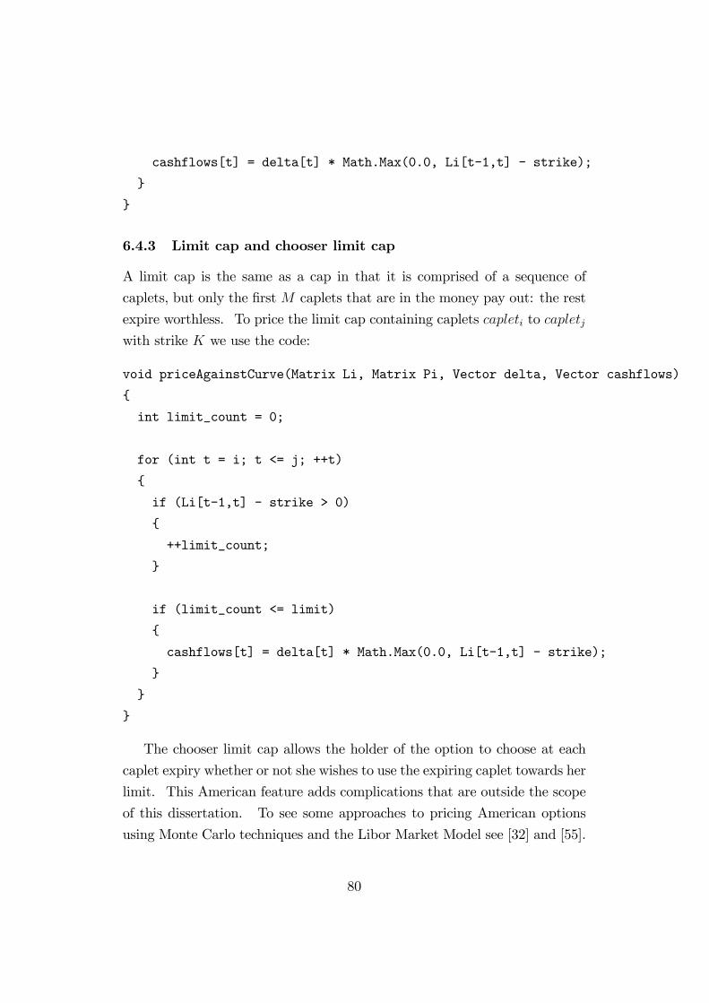
cashflows[t] = delta[t] * Math.Max(0.0, Li[t-1,t] - strike);
}
}
6.4.3 Limit cap and chooser limit cap
A limit cap is the same as a cap in that it is comprised of a sequence of
caplets, but only the �rst M caplets that are in the money pay out: the rest
expire worthless. To price the limit cap containing caplets capleti to capletjwith strike K we use the code:
void priceAgainstCurve(Matrix Li, Matrix Pi, Vector delta, Vector cashflows)
{
int limit_count = 0;
for (int t = i; t <= j; ++t)
{
if (Li[t-1,t] - strike > 0)
{
++limit_count;
}
if (limit_count <= limit)
{
cashflows[t] = delta[t] * Math.Max(0.0, Li[t-1,t] - strike);
}
}
}
The chooser limit cap allows the holder of the option to choose at each
caplet expiry whether or not she wishes to use the expiring caplet towards her
limit. This American feature adds complications that are outside the scope
of this dissertation. To see some approaches to pricing American options
using Monte Carlo techniques and the Libor Market Model see [32] and [55].
80
6.4.4 Barrier caplet
A barrier caplet is a path-dependent caplet that has either: a knockout
feature that causes the option to immediately terminate if the underlying
reaches a speci�c barrier level; or a knock-in feature that causes the option
to pay out only if the underlying has reached a speci�ed barrier level during
the lifetime of the option. It must be carefully stated in the option contract
how often the underlying is monitored for a breach of the barrier. Due to
the contingent nature of the option they tend to have lower prices than their
corresponding vanilla options.
To price a discrete knock-out barrier caplet with inspections of the un-
derlying for knock-out only on tenor dates we use the code:
void priceAgainstCurve(Matrix Li, Matrix Pi, Vector delta, Vector cashflows)
{
bool barrier_breached = false;
// Check for a breach in barrier
for (int j = 0; j < i; ++j)
{
if (Li[j,i+1] < down_barrier)
{
barrier_breached = true;
break;
}
}
// Define the payoffs only if the barrier was not breached
if (!barrier_breached)
{
cashflows[i] = delta[i] * Math.Max(0.0, Li[i-1,i] - strike);
}
}
81

Up to now we have priced only derivatives that work directly with the
forward rates and look and behave very much like the vanilla caplet. We
now move onto a set of products that work with swap rates.
6.4.5 Swaption
The formula for determining a swap rate in terms of the forward rates is (3).
The time Ti payo¤ a swaption on a swap with cash�ows from time Ti to time
TN is just the positive part of the value of the swap at time Ti minus the
strike price.
void priceAgainstCurve(Matrix Li, Matrix Pi, Vector delta, Vector cashflows)
{
int N = delta.cols;
// Calculate the swap rate
double w_denominator = 0.0;
for (int k = first_included_time; k < N; ++k)
{
w_denominator += delta[k]*Pi[first_included_time,k];
}
// Loop through the time periods that comprise the swap
double swap_rate = 0.0;
for (int j = first_included_time; j < N; ++j)
{
double w_numerator = delta[j] * Pi[first_included_time,j];
swap_rate += w_numerator / w_denominator * Li[first_included_time,j];
}
cashflows[first_included_time] = Math.Max(0.0, swap_rate - strike);
}
82

6.4.6 Trigger swap
The trigger-swap provides interest rate protection while ensuring full bene�t
if interest rates move in a desired direction. A trigger-swap is an agreement
whereby the borrower pays the lower of the Libor rate (plus some margin)
or a speci�ed �xed level. By entering into a trigger swap, the borrower may
bene�t from a decline in interest rates while still being protected against an
interest rate hike. The T0 value of the trigger swap on a nominal of 1 with
cash�ows from time Ti to TN can be calculated with the code:
void priceAgainstCurve(Matrix Li, Matrix Pi, Vector delta, Vector cashflows)
{
int N = delta.cols;
for (int i = first_included_time; i < N; ++i)
{
cashflows[i] = delta[i] * Math.Min(ceiling, Li[i-1, i]);
}
}
6.4.7 Bermudan swaption
Bermudan swaptions are probably the most popular of the exotic interest rate
products in the market as they are fundamental to the pricing of home loans
where the borrower can pay o¤ their loan early. This ability to settle a loan
at any time gives the holder of the loan an American (or Bermudan) option
on the underlying interest rate. This American feature adds complications
that are outside the scope of this dissertation. The pricing of Bermudan
swaptions is currently an area of active research: [2], [36], [38] and [52] treat
speci�cally the pricing of Bermudan swaptions using the Libor Market Model.
83

Ti �i Ti �i1 0.180253 11 0.1379822 0.191478 12 0.1347083 0.186154 13 0.1314284 0.177294 14 0.1281485 0.167887 15 0.1271006 0.158123 16 0.1268227 0.152688 17 0.1265398 0.148709 18 0.1262579 0.144703 19 0.12597010 0.141259
Table 1: 20 year caplet volatility view of the Banca IMI traders at 16 May2000
7 Results
This section presents the results of several experiments. They were im-
plemented in C# and run on a 3.0GHz Pentium 4 with 1Gb RAM. The
�rst four sections examine the issues around the calibration of volatility and
correlation matrices to caplets and swaptions and also the e¤ects of factor
reduction on the correlation matrix. Then Section 7.5 shows the e¤ect of
using di¤erent random number generators on the prices calculated by the
Monte Carlo method. Section 7.6 shows the various issues surrounding the
calculation of the Greeks. Section 7.7 shows that the Libor Market Model
generates the same price for di¤erent interest rate derivatives no matter our
choice of numeraire. Finally, Section 7.8 shows the prices of the various
options covered in Section 6.4.
7.1 Calibration to caplets
We �rst calibrate our model to some caplet market data using the method
described in Section 5.4. As was explained, caplet market data is generally
obtained from the trading desk. Table 1 shows the market data supplied
by [10], which contains the 20 year caplet volatility view of the Banca IMI
traders at 16 May 2000.
Figures 15 and 16 show the results of calibration to caplet market data.
84

Figure 15: Calibration of model volatility to market data using a speci�cationof the time-homogenous form (19).
Calibration using the Nelder-Mead takes a couple of seconds. The �rst �gure
shows how well the time-homogenous accumulated volatility parametrisation
(solid line) of the form in Equation (19) �ts the market data (circles). The
dashed line shows the corresponding instantaneous volatility. To be precise,
the solid line showsq
1T
R T0�2(u)du while the dashed line shows �(T ).
The resulting parameters for Equation (19) are:a = -0.0195607358161403 c = 0.959891548098344
b = 0.307959414926732 d = 0.103684750097087Naturally the parametrisation does not �t the market data exactly, es-
pecially in the term structure from years 13 to 16. Figure 16 shows the
resulting calibration once we add some time-inhomogeneity as proscribed by
Equation (21). Notice that the scaling factors Ki are very close to unity, as
we should like.
85
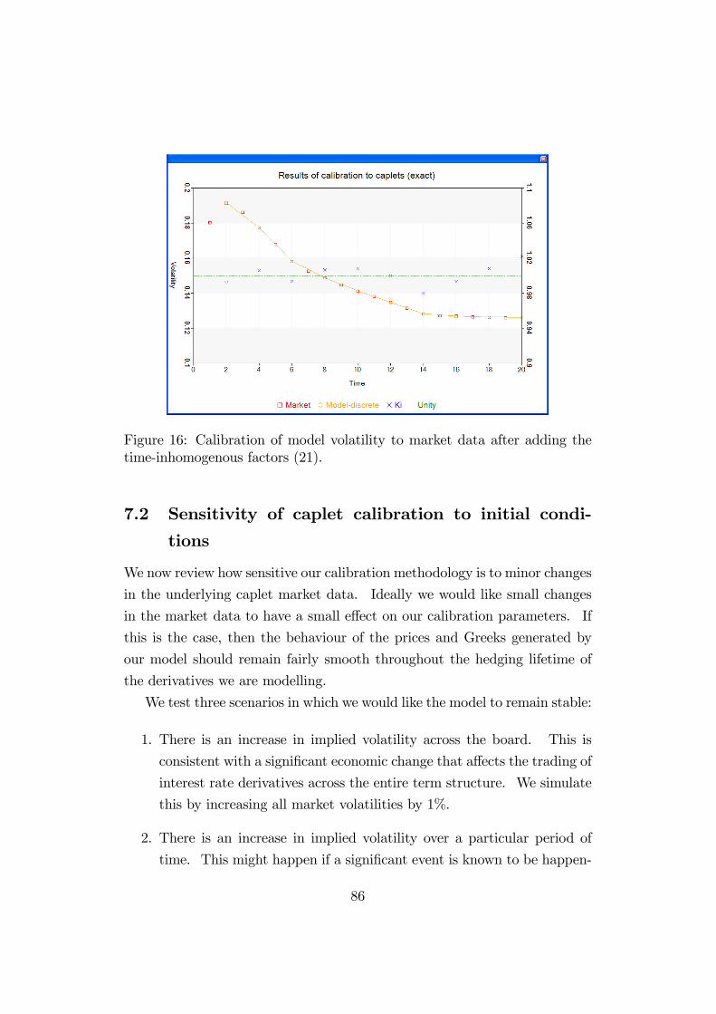
Figure 16: Calibration of model volatility to market data after adding thetime-inhomogenous factors (21).
7.2 Sensitivity of caplet calibration to initial condi-
tions
We now review how sensitive our calibration methodology is to minor changes
in the underlying caplet market data. Ideally we would like small changes
in the market data to have a small e¤ect on our calibration parameters. If
this is the case, then the behaviour of the prices and Greeks generated by
our model should remain fairly smooth throughout the hedging lifetime of
the derivatives we are modelling.
We test three scenarios in which we would like the model to remain stable:
1. There is an increase in implied volatility across the board. This is
consistent with a signi�cant economic change that a¤ects the trading of
interest rate derivatives across the entire term structure. We simulate
this by increasing all market volatilities by 1%.
2. There is an increase in implied volatility over a particular period of
time. This might happen if a signi�cant event is known to be happen-
86

a b c dOriginal -0.0195607 0.307959 0.959892 0.103685
Bumped up -0.0175795 0.302518 0.953801 0.114031Bumped up (few) -0.0121908 0.325393 0.951690 0.100538Bumped random -0.0195607 0.307959 0.959892 0.103685
Table 2: Parameters of the continuous time speci�cation after various changesto the caplet market data.
ing at a certain time, but the consequences of the event are not known.
We simulate this by increasing the market volatilities of the periods
from 2 to 5 years by 1%.
3. There are random changes in implied volatility. This might be con-
sistent with the normal market over time: market forces bump implied
volatilities by "random" amounts (the so-called volatility-of-volatility).
We simulate this by changing the market volatilities up or down by up
to 10% of their current value.
Figure 17 shows the resulting parameters which are listed in Table 2:
Notice that the parameters do not vary wildly across each scenario. Most
important is the fact that the random bumps of the market data yield a set
of parameters that is almost identical to the original set.
Figure 18 shows the term structures of volatility generated by the various
scenarios. Notice the line second-from-top, which corresponds to the 3 to
5 year bump in market vols: the model has done its best to capture these
bumps while matching the remaining values as closely as possible. The top
line shows the increase across the board of the market volatilities. The line
corresponding to the random bumps up and down is indistinguishable from
the original. This is very encouraging as it shows that the parametrisation
is robust in the presence of corrections to the market data.
Occasionally (about one out of every twenty runs), the Nelder-Mead al-
gorithm does not manage to �nd an optimal solution to the calibration. An
example is shown in Figure 19. It is important therefore to manually check
the results of the calibration routine to make sure that this has not happened.
87

Figure 17: Parameters of the continuous time speci�cation after variouschanges to the caplet market data.
Figure 18: Term structures of the calibrated market volatilities after variouschanges to the caplet market data.
88

Figure 19: An example of where the Nelder-Mead algorithm does not �ndan optimum solution during calibration.
If we require a completely automated system, we could run the calibration
routine several times and select the best solution.
7.3 Calibration to caplets and swaptions
Let us now see the e¤ect of calibrating the Libor Market Model to caplets
and swaptions in the market using the technique described in Section 5.5.
The design of the calibration requires that the availability of coherent caplet
and coterminal swaption market data, something I was not able to locate:
unfortunately [10] was missing values from years 7-9! To this end I have
"simulated" swaption volatility market data by calculating using Equation
(24) the swaption volatility that is implied by the caplet prices and then
bumped them down, giving swaption values that had similar shape to those
in [59]. This might yield market conditions that are not entirely realistic,
but it provides at least a dataset of market data against which we can test
the calibration method.
The �rst pair of series in Figure 20 show the caplet-implied and my
89
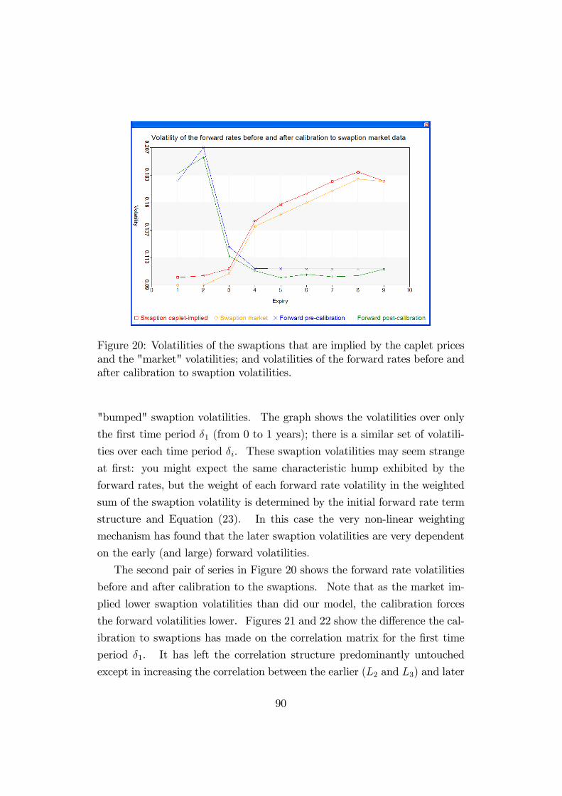
Figure 20: Volatilities of the swaptions that are implied by the caplet pricesand the "market" volatilities; and volatilities of the forward rates before andafter calibration to swaption volatilities.
"bumped" swaption volatilities. The graph shows the volatilities over only
the �rst time period �1 (from 0 to 1 years); there is a similar set of volatili-
ties over each time period �i. These swaption volatilities may seem strange
at �rst: you might expect the same characteristic hump exhibited by the
forward rates, but the weight of each forward rate volatility in the weighted
sum of the swaption volatility is determined by the initial forward rate term
structure and Equation (23). In this case the very non-linear weighting
mechanism has found that the later swaption volatilities are very dependent
on the early (and large) forward volatilities.
The second pair of series in Figure 20 shows the forward rate volatilities
before and after calibration to the swaptions. Note that as the market im-
plied lower swaption volatilities than did our model, the calibration forces
the forward volatilities lower. Figures 21 and 22 show the di¤erence the cal-
ibration to swaptions has made on the correlation matrix for the �rst time
period �1. It has left the correlation structure predominantly untouched
except in increasing the correlation between the earlier (L2 and L3) and later
90

Figure 21: Correlation of forward rates before calibration to swaptions in themarket. The �oor axes represent the year of expiry of the forward rates andthe vertical axis their correlation.
(L4 through L9) forward rates. This is shown more clearly in Figure 23,
where the correlation matrix after calibration to swaptions has been sub-
tracted from the initial correlation matrix.
7.4 Reduced factor matrices
This experiment determines the e¤ect of factor reduction on the prices of a
caplet and a swaption and on their computation time. In both simulations
the discount bond chosen as numeraire is that maturing in ten years. The
caplet runs from year 8 to year 9. The swaption expires on year 2 and lasts
till year 10. The initial forward curve and volatilities are not that important
for the results of this experiment and are chosen arbitrarily: the yield curve
is gently decreasing from 9% out to 10 years while the volatility curve is the
one calibrated in Section 7.1.
Figures 21 and 22 show, respectively, the correlation matrix before and
after calibration to swaptions. Figure 23 shows their di¤erence. Figure 24
91

Figure 22: Correlation of forward rates after calibration to swaptions in themarket. The �oor axes represent the year of expiry of the forward rates andthe vertical axis their correlation.
Figure 23: Di¤erences in the forward rate correlations before and after cali-bration to swaptions in the market.
92

Figure 24: The e¤ect of the number of factors on the price of a caplet. Thereis only a 0.01% di¤erence in price across simulations. The computation time(in seconds) is almost linear in the number of factors.
shows the e¤ect of factor reduction on the caplet price. There is hardly
any change in the caplet price (less than 0.01%) as we move from one to
ten factors. We should expect almost no change in the caplet price for
even one factor because factor reduction a¤ects only the correlation between
the forward rates: a caplet price is not in�uenced by correlation, only the
volatility of the forward rate prevailing over the lifetime of the option. Notice
though that the change in computation time is almost linear in the number
of factors.
Figure 25 shows the e¤ect of factor reduction on the swaption price.
There is a more signi�cant change in the swaption price (around 0.1%) as we
move from one to ten factors, with the most dramatic change arising from
one to four factors. After �ve factors there is little change to the swaption
price. We would expect this larger in�uence of the number of factors on
the swaption price because a swaption is sensitive to the correlation between
the forward rates prevailing over its entire lifetime. Again, the change in
computation time is almost linear in the number of factors.
93

Figure 25: The e¤ect of the number of factors on the price of a swaption.There is only a 0.1% di¤erence in price across simulations. The computationtime (in seconds) is almost linear in the number of factors.
7.5 E¤ect of di¤erent random number sources and an-
tithetics
Let us now turn to examining the e¤ect that the di¤erent random number
generators have on the pricing of derivatives. We have at our disposal three
sources of random numbers:
� pseudo-random numbers generated by the Mersenne Twister algorithm(presented in Section 6.2.1);
� pseudo-random numbers generated by the Mersenne Twister algorithmwith antithetic sampling (presented in Section 6.2.3); and
� quasi-random numbers generated by the Sobol sequences (presented inSection 6.2.2)
Figure 26 shows the results of pricing a caplet using the three di¤erent
sources of random numbers. Notice how the Sobol-driven simulation con-
verges very quickly, needing as few as 4096 iterations to have settled down
94

Figure 26: Illustration of the power of Sobol sequences and of antithetic vari-ables. Notice how the Sobol-driven simulation converges very quickly. Theantithetic-driven simulation seems to converge almost as quickly although itexhibits a slow drift upwards. The vanilla Mersenne-driven simulation hasterrible convergence characteristics.
95
around the option price. The antithetic-driven simulation seems to converge
almost as quickly although it exhibits a slow drift upwards: it has almost co-
incided with the Sobol-driven simulation by 16384 simulations. The vanilla
Mersenne-driven simulation has terrible convergence characteristics.
These results speak of the power of Sobol-driven Monte Carlo techniques:
although not truly random, their ability to quickly probe the broadest cross-
section of the simulation space ensures that they produce prices that take
into account most of the features of a derivative product. Obviously the
�ner features, e.g. the discontinuities caused by barrier options, would be
detected only as more iterations are performed and the Sobol number mesh
becomes small enough to approximate these features. Pseudo-random tech-
niques might uncover these �ner features sooner as they randomly sample
the simulation space, but in a probabilistic sense they are unlikely to �nd
them consistently sooner.
7.6 The Greeks
This experiment calculates the Greeks of three options: a caplet expiring
at T1 with payo¤ at T2; a caplet expiring at T3 with payo¤ at T4; and a
swaption expiring at T4 with payo¤s from times T5 to T10. The Greeks were
calculated using the di¤erent "bump" factors in the underlying forward rates
as discussed in Section 4.6: �Li = 4p"Li (as recommended by [29]); �Li =
0:01Li (1% recommended by [49]) and just for good measure �Li = 0:001Li(0.1%). I included the third factor to see just how sensitive our estimates of
the Greeks are to the choice of bump factors.
All three options were calculated using the T9 discount bond as numeraire
so that the caplets might be priced in the same framework as a 5-year swap-
tion starting in year 4.
Figure 27 shows the calculations for delta. Notice that the results using
any of the bump factors are all but identical. As we would expect, the caplet2option is sensitive primarily to L2 since its payo¤is directly dependent on that
forward rate. Obviously the rate L1 does not play an important enough role
in the discounting of the payo¤ to warrant a signi�cant sensitivity. However
96

the caplet4 option does show slight sensitivity to the rates L1 through L3:
they are used to discount the payment to the valuation time. As expected
the caplet4 option is very sensitive to L4. The swaption4 option is the
most interesting. It generates cash�ows from time T5 to T9 dependent on
the forward rates L5 to L9 and so is obviously going to have signi�cant
sensitivity to those forward rates. It is also rather sensitive to the forward
rates before its expiry, probably because of the discounting of the cash�ows,
but also because of the role they play in the calculation of the discount bonds
used in the valuation of the par swap rate in Equation (3).
Figure 28 shows the calculations for gamma. Here we start seeing in-
stabilities in the calculated values depending on the size of the bump factor.
Indeed, using the 4p" bump factor yields results that are completely unstable
(in the order of 106) and so have been omitted. There is a slight di¤erence
between the values of gamma calculated using 1% and 0.1% bump factors
and it is not clear which values might be the correct ones to use when hedg-
ing. It might be reasonable for the hedging trader to estimate the size of
jump in underlying forward price that she would expect before hedging and
use that number to calculate gamma. We see sensitivities to the underlying
forward rates similar to those of delta.
7.7 E¤ect of di¤erent numeraires on accuracy
This experiment tests that our change of numeraire mathematics is correct:
Equation (13) gives us the dynamics of our forward rates under any choice of
discount bond as numeraire. This means that we should calculate the same
price for a derivative no matter which discount bond we use as numeraire.
Figure 29 shows us the calculated price of a caplet with expiry at the
end of year 1 and payment at the end of year 2 when priced under di¤erent
discount bond numeraires with expiries ranging from 4 years to 20 years.
Notice that the price does indeed remain relatively constant (at least to
within 0.1%). What we also expect is an increase in the variance of this
price: as we push the numeraire further out in time we have to carry our
caplet cash�ow at year 3 forward through many more simulated forward
97
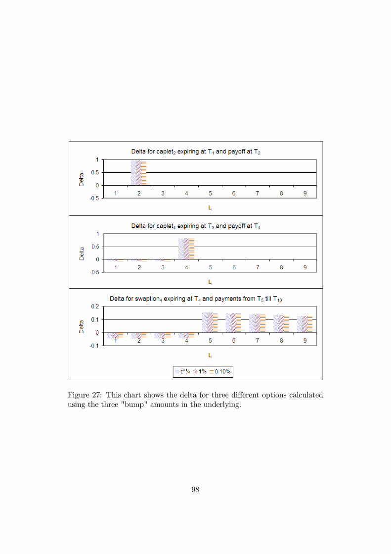
Figure 27: This chart shows the delta for three di¤erent options calculatedusing the three "bump" amounts in the underlying.
98

Figure 28: This chart shows the gamma for three di¤erent options calculatedusing the three "bump" amounts in the underlying. Note that the valuescalculated using 4
p" as the bump amount were completely unstable (in the
order of 106) and so have been omitted.
99

Figure 29: Notice that the choice of numeraire has little impact on the price ofthe derivative, although there is an increase in the variance of our simulationestimate.
rates to our terminal measure and then discount it back to today. The e¤ect
of the additional variance of each simulated forward rate should cause the
derivative variance to increase too. This is evident in Figure 29.
7.8 Pricing various options
For completeness, Figure 30 shows the prices and Greeks of various interest
rate derivatives priced using the Libor Market Model. Although we done go
into much detail about the properties of these derivative prices and have not
even shown the initial forward curve nor the forward volatilities that got us
to these prices, it is instructive to do some brief inspection of the results:
� Notice that the down-and-out caplet is cheaper than the correspondingcaplet, as we would expect from an option that might become worthless.
� Notice that the limit cap is cheaper than the corresponding cap as itprovides only 2 out of the 6 payo¤s that does the ordinary cap.
100

� The two caplet types are sensitive only to the underlying forward rateat their expiry (on which their payo¤is contingent), whereas the caplets
are (obviously) sensitive to all the forward rates they span. Interesting
is the fact that the limit cap with two payo¤s is sensitive to the �rst two
forward rates it spans and hardly sensitive to the third: this must mean
that the comprising caplets are rather in the money and will likely be
exercised.
� The swaption is sensitive to all the forward rates it spans while thetrigger swap is sensitive only to the �rst few. It is negatively correlated
to movements in the latter forward curves: these must be high enough
to trigger the �xed swap payment and so their value is re�ected only
in the discounting of the later cash�ows.
101

Figure 30: The price and Greeks of various options priced using the LiborMarket Model.
102
8 Conclusion
The intention of this dissertation was to draw from the literature to bring into
one body of work a treatment of the Libor Market Model from start to �nish
so that the reader might understand the basics of the Libor Market Model
and implement the model without having to piece together information from
other sources. Has this been achieved? Certainly the derivation of the
mathematical model in Section 4 has distilled work from several sources into
a consistent notational framework. The sandy areas in the mathematical
model where it is left to the implementor to choose speci�c speci�cations
for volatility, correlation, choices of factors, Monte Carlo details were set in
concrete in Sections 5 and 6. And �nally, Section 7 showed that the model,
as implemented, works as hypothesised without any nasty surprises.
The achievement of the programming e¤ort of several thousand lines of
code is the simple interface that one needs to implement to price a new inter-
est rate product. One needs simply to describe the cash�ows of the derivative
to price it. The calibration, factor reduction, Monte Carlo simulations, cal-
culation of Greeks and everything else that goes into the implementation of
the Libor Market Model is done behind the scenes.
The model has shown itself to be extremely �exible in its ability to cal-
culate the prices and Greeks of a wide variety of options with minimal e¤ort.
The beautiful simplicity of the model ensures that it can be easily under-
stood and quickly and correctly implemented. As computers become faster,
the time it takes to perform the Monte Carlo simulations will drop, allowing
even more complex derivatives to be priced without having to make signi�-
cant changes to the model or code.
There are obviously some shortcomings of the model, but they are by
no means insurmountable. The pricing of American or Bermudan options
poses challenges to any model relying on Monte Carlo techniques: signi�-
cant progress has been made in improving this state of a¤airs, especially in
the case of Bermudan options. The calculation of the Greeks using a gen-
eral �nite di¤erence approach is risky when there are discontinuities in the
option payo¤s - especially those of path dependent options: techniques like
103

the pathwise method and the likelihood ratio method help to resolve this,
although in their current form they can not be applied to general options
without individual changes to their code. Computation time can become a
problem, especially when calculating the sensitivities of long-term options to
each of the many forward rates they span: distributed computing techniques
(to which Monte Carlo methods are particularly suited) can help alleviate
this problem by sharing the load across many computers.
In addition to the active research being done where the Libor Market
Model has its shortcomings, there is signi�cant work being done to advance
the Libor Market Model to take into account skews and smiles in the in-
terest rate volatilities; to take advantage of developments in Levy and jump
processes; and into using vast computing grids to use the Libor Market Model
to risk manage portfolios of thousands of derivatives. All these areas provide
scope for some very interesting further research.
104

9 Bibliography
References
[1] Alexander, C.; Common Correlation and Calibrating the Lognormal For-
ward Rate Model; Wilmott Magazine; March 2003 pp68-78; 2003
[2] Andersen, L.; A simple approach to the pricing of Bermudan swaptions
in the multifactor LIBOR market model; Journal of Computational Fi-
nance; 3.2 pp5-32; 2000
[3] Björk, T.; Arbitrage Theory in Continuous Time; Second Edition; Ox-
ford University Press; 2004
[4] Brace, A., Gatarek, D. & Musiela, M.; The market model of interest
rate dynamics; Mathematical Finance; 7 pp127-155; 1997
[5] Black, F.; The Pricing of Commodity Contracts; Journal of Financial
Econometrics; 3 pp167-179; 1976
[6] Black, F., Derman, E. & Toy, W.; A one-factor model of interest rates
and its application to treasury bond options; Financial Analysts Journal;
pp33-39; 1990
[7] Boyle, P., Broadie, M. & Glasserman, P.; Monte Carlo methods for
security pricing; Journal of Economic Dynamics and Control; 21 pp1267-
1321; 1997
[8] Brigo, D.; A note on correlation and rank reduction; Banca IMI Working
Paper; www.damianobrigo.it; 2002
[9] Brigo, D. & Mercurio, F.; Calibrating LIBOR; Risk Magazine; January
issue pp117-121; 2002
[10] Brigo, D., Mercurio, F. & Morini, M.; Di¤erent Covariance Parame-
terizations of the Libor Market Model and Joint Caps/Swaptions Cali-
bration; Product and Business Development Group Banca IMI working
paper; 2003
105

[11] Brigo, D., Mercurio, F. & Morini, M.; The Libor model dynamics: Ap-
proximations, calibration and diagnostics; European Journal of Opera-
tional Research; 163 pp30�51; 2005
[12] Broadie, M.; Glasserman, P.; Estimating Security Price Derivatives Us-
ing Simulation; Management Science; 42.2 pp269-285; 1996
[13] Cairns, A.J.G.; Interest Rate Models: An Introduction; Princeton Uni-
versity Press; 2004
[14] Co¤ey, B. & Schönmakers, J.; Stable implied calibration of a multi-factor
Libor model via a semi-parametric correlation structure; Working paper
611; Weierstrass-Institut für Angewandte Analysis und Stochastik; 2000
[15] Co¤ey, B. & Schönmakers, J.; Systematic generation of parametric cor-
relation structures for the Libor Market Model; International Journal of
Theoretical and Applied Finance; 6.5 pp507-519; 2003
[16] Cox, J.C., Ingersoll, J.e. & Ross, S.A.; An intertemporal general equi-
librium model of asset prices; Econometrica; 53 pp363-384; 1985
[17] Derman, E.; My Life as a Quant: Re�ections on Physics and Finance;
John Wiley and Sons; 2004
[18] Glasserman, P.; Monte Carlo Methods in Financial Engineering;
Springer; 2004
[19] Glasserman, P. & Zhao, X.; Fast Greeks by simulation in forward LIBOR
models; Journal of Computational Finance; 3 pp5-39; 1999
[20] Glasserman, P. & Zhao, X.; Arbitrage-free discretization of lognormal
forward Libor and swap rate models; Finance and Stochastics; 4 pp35-
68; 2000
[21] Grubi�ic, I. & Pietersz, R.; E¢ cient rank reduction of
correlation matrices; Working paper; Utrecht University;
www.few.eur.nl/few/people/pietersz; 2004
106

[22] Hagan, P. & West, G.; Interpolation Methods for Curve Construction;
Working paper, to appear in Applied Mathematical Finance; 2005
[23] Harrison, J.M. & Pliska, S.; Martingales and stochastic integrals in the
theory of continuous trading; Stochastic Processes and their Applica-
tions; 11 pp215-260; 1981
[24] Heath, D., Jarrow, R. & Morton, A.; Bond pricing and the term struc-
ture of interest rates: A new methodology for contingent claims valua-
tion; Econometrica; 60 pp77-105; 1992
[25] Ho, T.S.Y. & Lee, S.B.; Term structure movements and pricing interest
rate contingent claims; Journal of Finance; 41; 1986
[26] Hull, J.C.; Options, Futures, and Other Derivatives; Fifth Edition; Pren-
tice Hall; 2003
[27] Hull, J.C. &White, A.; Pricing interest rate derivative securities; Review
of Financial Studies; 3; 1990
[28] Hunt, P.J. & Kennedy, J.E.; Financial Derivatives in Theory and Prac-
tice; Revised Edition; John Wiley and Sons; 2004
[29] Jäckel, P.; Monte Carlo Methods in Finance; John Wiley and Sons; 2002
[30] Jamshidian, F.; Libor and swap market models and measures; Finance
and Stochastics; 1 pp293�330; 1997
[31] Joshi, M.S.; A short note on exponential correlation functions; QUARC
Royal Bank of Scotland working paper; 2000
[32] Joshi, M.S.; The Concepts and Practice of Mathematical Finance; Cam-
bridge University Press; 2003
[33] Jäckel P. & Rebonato R.; Accurate and optimal calibration to
co-terminal European swaptions in a FRA-based BGM framework;
QUARC Royal Bank of Scotland working paper; 2000
107
[34] Jäckel P. & Rebonato R.; Linking Caplet and Swaption Volatilities in
a BGM/J Framework: Approximate Solutions; QUARC Royal Bank of
Scotland working paper; 2000
[35] Jäckel P. & Rebonato R.; The Link between Caplet and Swaption
Volatilities in a BGM/J Framework; Journal of Computational Finance;
6.4 pp41-59; 2003
[36] Joshi, M.S. & Theis, J.; Bounding Bermudan swaptions in a swap-rate
market model; Quantitative Finance; 2 pp370-377; 2002
[37] Kloeden, P.E. & Platen, E.; Numerical Solution of Stochastic Di¤erential
Equations; Springer; 1992
[38] Kolodko, A. & Schoenmakers, J.; Iterative construction of the optimal
Bermudan stopping time; Financial Engineering and Applications; 2004
[39] Longsta¤, F.A. & Schwartz, E.S.; Interest rate volatility and the term
structure: A two-factor general equilibrium model; Journal of Finance;
47; 1992
[40] Longsta¤, F., Santa-Clara, P. & Schwartz, E.; The Relative Valuation
of Caps and Swaptions: Theory and Empirical Evidence; Journal of
Finance; 56.6 pp2067�2109; 2000
[41] Matsumoto, M. & Nishimura, T.; Mersenne twister: a 623-dimensionally
equidistributed uniform pseudo-random number generator; ACM Trans-
actions on Modeling and Computer Simulation (TOMACS); 8:1 pp3-30;
1998
[42] Merton, R.C.; Theory of Rational Option Pricing; Bell Journal of Eco-
nomics and Management Science; 4 pp141-183; 1973
[43] Meyer, M.J.; The Martingale Project; http://martingale.berlios.de;
2003
108

[44] Mikosch, T.; Elementary Stochastic Calculus with Finance in View; Ad-
vanced Series on Statistical Science & Applied Probability Vol. 6; World
Scienti�c; 1998
[45] Milterstein, M., Sandmann, K. & Sondermann, D.; Closed-form solu-
tions for term structure derivatives with lognormal interest rates; Jour-
nal of Finance; pp409-430; 1997
[46] Musiela, M. & Rutkowski, M.; Continuous-time term structure models:
Forward measure approach; Finance and Stochastics; 1 pp261-291; 1997
[47] Niederreiter, H.; Low-discrepancy sequences and global function �elds
with many rational places; Finite Fields and their Applications; 2 pp241-
273; 1996
[48] Øksendal, B.; Stochastic Di¤erential Equations: An Introduction with
Applications; Fifth Edition; Springer; 2000
[49] Panday, S.; E¢ cient Simulation within the LIBOR Market Model; Mas-
ter�s Degree in Econometrics and Operations Research, Vrije Universiteit
Amsterdam; 2003
[50] Pelsser, A.; E¢ cient Methods for Valuing Interest Rate Derivatives;
Springer; 2000
[51] Piterbarg, V.; A Practitioner�s Guide to Pricing and
Hedging Callable Libor Exotics in Forward Libor Models;
http://ssrn.com/abstract=427084; 2003
[52] Pietersz, R. & Pelsser, A.; Risk Managing Bermudan Swaptions in the
Libor BGM Model; Journal of Derivatives; 11.3 pp51�62; 2004
[53] Pietersz, R. & Pelsser, A.; Swap Vega in BGM: Pitfalls and Alternatives;
Risk 17 (March04) pp91-93; 2004
[54] Press, W.H., Teukolsky, S.A., Vetterling, W.T. & Flannery, B.P.; Nu-
merical Recipes in C: The Art of Scienti�c Computing; Second Edition;
Cambridge University Press; 1992
109

[55] Rebonato R.; Interest-rate option models; Second Edition; John Wiley
and Sons; 1996
[56] Rebonato R.; On the pricing implications of the joint log-normality as-
sumption for the cap and swaption markets; Journal of Computational
Finance; 2.3 pp30-52; 1999
[57] Rebonato R.; Volatility and correlation; John Wiley; 1999
[58] Rebonato R.; Accurate and optimal calibration to co-terminal European
swaptions in a FRA-based BGM framework; QUARC Royal Bank of
Scotland working paper; 2000
[59] Rebonato, R.; Modern Pricing of Interest Rate Derivatives; Princeton
University Press; 2002
[60] Sidenius, J.; Libor Market Models in practice; Journal of Computational
Finance; 3.3 pp75-99; 2000
[61] Sobol, I.M.; On the distribution of points in a cube and the approx-
imate evaluation of integrals; USSR Computational Mathematics and
Mathematical Physics; 7 pp86-112; 1967
[62] Svoboda, S.; An Investigation of Various Interest Rate Models and their
Calibration in the SA Market; MSc Dissertation; University of the Wit-
watersrand; 2002
[63] Vasicek, O.; An Equilibrium Characterisation of the Term Structure;
Journal of Financial Econometrics; 5 pp177-188; 1977
[64] West, G.; Better Approximations to Cumulative Normal Functions;
Wilmott Magazine; May 2005 pp70-76; 2005
[65] Wilmott, P.; Derivatives: The Theory and Practise of Financial Engi-
neering; John Wiley and Sons; 1998
[66] Wilmott, P.; Paul Wilmott on Quantitative Finance; John Wiley and
Sons; 2000
110

10 Code Appendix
The source code implemented during the development of this dissertation is
available online at http://www.jimme.net. Including the thousands of lines
of source code as an appendix seemed somewhat counterproductive. Instead,
included are a few snippets of code that are useful enough to warrant being
published in print, not readily available in the literature, and concise enough
to make a reasonable appendix.
10.1 IntegratingR ts �i(u)�j(u)du
To calculateR ts�i(u)�j(u)du use:
public double getIntegralDefinite(double s, double t, double Ti, double Tj)
{
return getIntegralIndefinite(t, Ti, Tj) - getIntegralIndefinite(s, Ti, Tj);
}
public double getIntegralIndefinite(double t, double Ti, double Tj)
{
double ctmTi=c*(t-Ti);
double ctmTj=c*(t-Tj);
double q=ctmTi+ctmTj;
double ac=a*c;
double cd=c*d;
double f=1.0/(c*c*c);
double A=ac*cd*(exp(ctmTj)+exp(ctmTi))+c*cd*cd*t;
double B=b*cd*(exp(ctmTi)*(ctmTi-1)+exp(ctmTj)*(ctmTj-1));
double C=exp(q)*(ac*(ac+b*(1-q))+b*b*(0.5*(1-q)+ctmTi*ctmTj))/2;
return f*(A-B+C);
}
111

10.2 Moro�s Normal inverse transform
Moro�s algorithm is used to convert a uniformly distributed number in the
range [0; 1] to a Normally distributed number in the range [�1;1]. It
is purportedly accurate to 14 decimal places, although I would be a little
sceptical out in the tails of the distribution.
public static double InvDist_SN_Moro(double y)
{
double zz;
double z = y - 0.5;
if (Math.Abs(z) < 0.42)
{
zz = Math.Pow(z,2);
zz = z * (((-25.44106049637 * zz + 41.39119773534)
* zz + -18.61500062529) * zz + 2.50662823884) /
((((3.13082909833 * zz + -21.06224101826) * zz + 23.08336743743)
* zz + -8.4735109309) * zz + 1);
}
else
{
if (z > 0) zz = Math.Log(-Math.Log(1 - y));
else zz = Math.Log(-Math.Log(y));
double build = 2.888167364E-07 + zz * 3.960315187E-07;
build = 3.21767881768E-05 + zz * build;
build = 3.951896511919E-04 + zz * build;
build = 3.8405729373609E-03 + zz * build;
build = 2.76438810333863E-02 + zz * build;
build = 0.160797971491821 + zz * build;
build = 0.976169019091719 + zz * build;
zz = 0.337475482272615 + zz * build;
112

if (z <= 0) zz = -zz;
}
return zz;
}
10.3 The Nelder-Mead algorithm
The Nelder-Mead algorithm is an optimisation algorithm for �nding a global
minimum in a highly non-linear and non-di¤erentiable search space. It comes
in two parts: the ObjectiveFunction interface, which must be implemented
to evaluate and constrain the objective function at the point p; and the
NelderMead class, which performs the actual optimisation.
using System;
namespace Utilities.Mathematics.Optimisation.NelderMead
{
public interface ObjectiveFunction
{
double evaluate(double[] p);
void constrainSearch(ref double[] p);
}
}
using System;
namespace Utilities.Mathematics.Optimisation.NelderMead
{
public class NelderMead
{
const double GROW_FACTOR = 2.0;
const double REFLECT_FACTOR = -1.0;
const double CONTRACT_FACTOR = 0.5;
113

const double SHRINK_FACTOR = 0.5;
public double MAX_ITERATIONS = 10000;
public double TOLERANCE = 1E-12;
int dimensions;
ObjectiveFunction objective_function;
double[][] points;
double[] scores;
public NelderMead(int adimensions)
{
dimensions = adimensions;
points = new double[dimensions+1][];
for (int i = 0; i < dimensions+1; ++i)
{
points[i] = new double[dimensions];
}
scores = new double[dimensions+1];
}
public double[][] generateEmptyStartupParameters(double[] scales)
{
Utilities.Random.RandomAugmented ra =
Utilities.Random.RandomAugmented.getSeededRandomAugmented();
double[][] initial_points = new double[dimensions+1][];
for (int i = 0; i < dimensions+1; ++i)
{
initial_points[i] = new double[dimensions];
for (int j = 0; j < dimensions; ++j)
{
initial_points[i][j] = ra.NextDoubleBalanced(scales[j]);
114

}
}
return initial_points;
}
public void initialiseSearch(ObjectiveFunction aobjective_function,
double[][] starting_points)
{
objective_function = aobjective_function;
// Store our initial conditions
for (int i = 0; i < dimensions+1; ++i)
{
for (int j = 0; j < dimensions; ++j)
{
points[i][j] = starting_points[i][j];
}
}
// Evaluate our initial conditions
for (int i = 0; i < dimensions+1; ++i)
{
scores[i] = objective_function.evaluate(points[i]);
}
sortPoints();
}
public double[] search(out string error_message, out double optimum_score)
{
// Check that we have been initialised
if (null == objective_function)
{
115

throw new
GenericException("Objective function not set. Can not search.");
}
// Initialise the error message
error_message = "";
// Keeps track of how many iterations we have done
int num_iterations = 0;
// The latest midpoint and newpoint we have for reflections, etc.
// Defined here for memory allocation efficiency
double[] mid_point = new double[dimensions];
double[] new_point = new double[dimensions];
while (true)
{
// Check our tolerance. If we are within it, return
double tolerance = 0.0;
for (int j = 0; j < dimensions; ++j)
{
tolerance += Math.Abs(points[0][j] - points[dimensions][j]);
}
tolerance /= dimensions;
if (tolerance < TOLERANCE)
{
optimum_score = scores[0];
return points[0];
}
// Check that we have not exceeded the number of iterations
++num_iterations;
if (num_iterations > MAX_ITERATIONS)
116

{
error_message =
"Exceeded number of iterations in the Nelder-Mead search. Results may be unstable!";
optimum_score = scores[0];
return points[0];
}
// Find the mid point of the best points (note n points, not n+1,
// since we leave out the worst)
for (int j = 0; j < dimensions; ++j)
{
mid_point[j] = 0.0;
}
for (int i = 0; i < dimensions; ++i)
{
for (int j = 0; j < dimensions; ++j)
{
mid_point[j] += points[i][j];
}
}
for (int j = 0; j < dimensions; ++j)
{
mid_point[j] /= dimensions;
}
// Do a reflection test
if (testOnePointMove(REFLECT_FACTOR, ref mid_point, ref new_point))
{
// If we managed a reflection, test a little further out
testOnePointMove(GROW_FACTOR, ref mid_point, ref new_point);
}
// If the reflection failed, then try a contraction
117

else if (testOnePointMove(CONTRACT_FACTOR, ref mid_point, ref new_point))
{
}
// If reflection and contraction failed, then shrink towards
// our best point
else
{
doManyPointMove();
}
}
}
void doManyPointMove()
{
for (int i = 1; i < dimensions+1; ++i)
{
for (int j = 1; j < dimensions; ++j)
{
points[i][j] = SHRINK_FACTOR * (points[i][j] + points[0][j]);
}
objective_function.constrainSearch(ref points[i]);
scores[i] = objective_function.evaluate(points[i]);
}
sortPoints();
}
bool testOnePointMove(double scale, ref double[] mid_point,
ref double[] new_point)
{
// Calculate our new point dimensions
for (int j = 0; j < dimensions; ++j)
118

{
new_point[j] = mid_point[j] +
scale * (points[dimensions][j] - mid_point[j]);
}
// Make sure our new point obeys the constraints
objective_function.constrainSearch(ref new_point);
// See if our new point is better
double new_score = objective_function.evaluate(new_point);
// If it is, replace our old point and return true
if (new_score < scores[dimensions])
{
for (int j = 0; j < dimensions; ++j)
{
points[dimensions][j] = new_point[j];
}
scores[dimensions] = new_score;
sortPoints();
return true;
}
// If it is not smaller, return false
else
{
return false;
}
}
void sortPoints()
119

{
// Lets do a simple bubble sort
// This can be improved since the only unsorted one is usually at
// the end of the array. But its probably not worth it cos there
// are always so few dimensions
for (int i = 0; i < dimensions; ++i)
{
for (int j=i+1; j < dimensions+1; ++j)
{
if (scores[i] > scores[j])
{
swapPoints(i, j);
}
}
}
}
void swapPoints(int a, int b)
{
Utilities.Swap.swap(ref scores[a], ref scores[b]);
for (int j = 0; j < dimensions; ++j)
{
Utilities.Swap.swap(ref points[a][j], ref points[b][j]);
}
}
}
}
10.4 The Mersenne Twister algorithm
The Mersenne Twister algorithm is useful for generating pseudo-random uni-
formly distributed numbers with excellent "random" properties in a machine
independent manner.
120

using System;
using Utilities.GUI.Charting;
using Utilities.Mathematics.LinearAlgebra;
namespace Utilities.Random
{
/**
* This class is an implementation of the paper "Mersenne Twister:
* A 623-Dimensionally Equidistributed Uniform Pseudo-Random Number Generator"
* by Matsumoto
*/
public class MersenneTwister : IUniformRandomSource
{
const int N = 624;
const int M = 397;
const uint MATRIX_A = 0x9908b0df;
const uint UPPER_MASK = 0x80000000;
const uint LOWER_MASK = 0x7fffffff;
const uint TEMPERING_MASK_B = 0x9d2c5680;
const uint TEMPERING_MASK_C = 0xefc60000;
ulong[] mt = new ulong[N];
int mti = N+1;
ulong[] mag01 = {0, MATRIX_A};
const ulong DEFAULT_SEED = 4357;
ulong seed_used;
public MersenneTwister()
{
SeedMT(DEFAULT_SEED);
}
public MersenneTwister(ulong seed)
121

{
if (0 == seed)
{
throw new Utilities.GenericException("Seed can not be zero.");
}
SeedMT(seed);
}
public void reset()
{
SeedMT(seed_used);
}
private void SeedMT(ulong seed)
{
seed_used = seed;
mt[0] = seed & 0xffffffff;
for (mti = 1; mti < N; ++mti)
{
mt[mti] = (69069 * mt[mti-1]) & 0xffffffff;
}
}
public ulong RandomInt()
{
ulong y;
if (mti >= N)
{
int kk;
for (kk = 0; kk < N-M; ++kk)
122

{
y = (mt[kk] & UPPER_MASK) | (mt[kk+1] & LOWER_MASK);
mt[kk] = mt[kk+M] ^(y >> 1) ^mag01[y&0x1];
}
for (;kk < N-1; ++kk)
{
y = (mt[kk] & UPPER_MASK) | (mt[kk+1] & LOWER_MASK);
mt[kk] = mt[kk+(M-N)] ^(y >> 1) ^mag01[y&0x1];
}
y = (mt[N-1] & UPPER_MASK) | (mt[0] & LOWER_MASK);
mt[N-1] = mt[M-1] ^(y >> 1) ^mag01[y&0x1];
mti = 0;
}
y = mt[mti++];
y ^= (y >> 11);
y ^= (y << 7) & TEMPERING_MASK_B;
y ^= (y << 15) & TEMPERING_MASK_C;
y ^= (y >> 18);
return y;
}
public double RandomDouble()
{
return ((double) RandomInt() / (double) 0xffffffff);
}
public void RandomUniformVector(Vector vector)
{
123
for (int i = 0; i < vector.cols; ++i)
{
vector[i] = RandomDouble();
}
}
public double nextRandomDouble()
{
return RandomDouble();
}
}
}
124