an experimental investigation of convection heat transfer
TRANSCRIPT

An experimental investigation of convection heat transferduring filling of a composite-fibre pressure vessel at lowReynolds number
Author
Heath, Melissa, Woodfield, Peter Lloyd, Hall, Wayne, Monde, Masanori
Published
2014
Journal Title
Experimental Thermal and Fluid Science
DOI
https://doi.org/10.1016/j.expthermflusci.2014.02.001
Copyright Statement
© 2014 Elsevier Inc. This is the author-manuscript version of this paper. Reproduced inaccordance with the copyright policy of the publisher. Please refer to the journal's website foraccess to the definitive, published version.
Downloaded from
http://hdl.handle.net/10072/62415
Griffith Research Online
https://research-repository.griffith.edu.au

An experimental investigation of convection heat transfer during filling of a composite-fibre
pressure vessel at low Reynolds number
Melissa Heath
School of Engineering, Griffith University
Gold Coast Campus, Qld, 4222, Australia
E-mail: [email protected]
Peter Lloyd Woodfield, (corresponding author)
School of Engineering, Griffith University
Gold Coast Campus, Qld, 4222, Australia
E-mail: [email protected]
TEL: +61-7-5552-7501
Wayne Hall
School of Engineering, Griffith University
Gold Coast Campus, Qld, 4222, Australia
E-mail: [email protected]
TEL: +61-7-5552-9278
Masanori Monde
Department of Mechanical Engineering, Saga University
1 Honjo-machi, Saga, 840-8502, Japan
E-mail: [email protected]

Abstract
The heat transfer process during filling of an evacuated vessel at low Reynolds number was
investigated experimentally using air as the flow medium. The data was analysed using a
thermodynamic model similar to one currently in use for the design of systems using commercial
carbon fibre reinforced plastic vessels for storage of compressed hydrogen gas. Model assumptions
included perfectly-stirred conditions within the vessel, one-dimensional unsteady heat conduction
through the composite vessel wall, ideal gas and frictional adiabatic flow conditions through the inlet
tube. A transition phenomenon from laminar to turbulent flow was observed by decreasing the inlet
diameter while maintaining a similar mass flow rate. Based on the measurements, a new empirical
correlation for the Nusselt number under low Reynolds number flow conditions is proposed.
Keywords: convection heat transfer correlation; composite pressure vessel

Nomenclature
a = thermal diffusivity
A = inside area of vessel
c = sound speed of air
cs = specific heat for solid
Cp = constant pressure specific heat of gas
d = internal diameter of supply pipe
D = internal diameter of experimental vessel
g = acceleration due to gravity
H = internal height of vessel
ha = specific internal enthalpy of supply
hf = head loss due to friction in supply pipe
L = length of supply pipe
m = mass of gas in vessel
M = Mach number
M& = mass flow rate
Nu = Nusselt number
P = Pressure in vessel
r = radial position in the wall
Ra = Rayleigh number
Re = Reynolds Number
Rair = ideal gas specific to air
Rcyl = internal radius of cylinder
Rin = inner radius

Rout = outer radius
t = time
tw = thickness of vessel wall
Ta = supply temperature of gas
Te = environment temperature
Tg = gas temperature
To = initial temperature of gas
Ts= temperature of solid
Tw = inside temperature of wall
u = specific internal energy
v = velocity in supply pipe
V = internal volume of vessel
Vf = Volume fibre fraction
Greek
αe = convection heat transfer coefficient from outside wall to environment
αh = convection heat transfer coefficient from gas to the wall
β = volumetric thermal expansion coefficient
λ = thermal conductivity
ν = Poisson’s ratio
µ = dynamic viscosity
ρ = density
τ = Fourier number = atRcyl-2

1. Introduction
This study is part of a larger investigation to explore heat transfer processes that occur during
pressurizing and depressurizing of gas containment vessels. The theme has particular importance for
carbon fibre reinforce plastic vessels used in fuel cell vehicles which have problems with overheating
during the semi-adiabatic compression process during filling [1-8]. Other applications include
accidental depressurization where the concern may be excessive internal cooling of a metal container
[9] and predictions of gas leakage rates from vessels [10]. For mobile applications, vessel sizes
typically range from a few litres suitable for hydrogen powered scooters or bicycles [11] to banks of
200 litre vessels used in fuel cell buses [12]. For applications which require very small vessels, metal
hydride hydrogen storage has been given relatively more attention than compressed storage in the
literature based on the perception that it is safer [13]. Compressed gas storage is still the most popular
choice for commercial hydrogen fuel cell cars.
When filling pressure vessels with compressed gas, flow work is done in the container which causes
heating. In the case of carbon fibre reinforced plastic (CFRP) vessels it becomes particularly
important to be able to predict the temperature rise since the material is sensitive to high temperatures.
A number of studies have considered computational fluid dynamics (CFD) modelling [3-6] and
experimentation where the temperature during filling was monitored [7, 8]. Somewhat surprisingly,
most research has focused on the temperature of the gas rather than the temperature distribution in the
vessel wall and there appears to be a lack of fundamental data describing the heat transfer process.
Very little attention has been given to heat transfer in this flow situation at low Reynolds number.
Recently, Winters et al. [14] experimentally and numerically investigated heat transfer during
depressurization of a spherical vessel. They found good agreement between their results and an
analytical model by Paolucci [15] during the early stages of gas expansion followed by a period of
time where natural convection heat transfer dominated. Charton et al. [9] considered the flow of gas
into an evacuated vessel connected to a pressurized vessel via a thin tube. Their experimental data was
in reasonable agreement with predictions from a thermodynamic model which utilized a natural
convection heat transfer correlation for both the supply vessel and the receiver. In their model, the
correlation used for the Nusselt number was of the form nCRaNu = where C is a constant and n is
approximately 0.25 for laminar natural convection and 1/3 for turbulent natural convection [16, 17].
Woodfield et al. [18], in their study on depressurizing and pressurizing of gas storage vessels, found
that heat transfer during filling of the vessel was better described using a mixed convection heat
transfer correlation involving both the inlet tube Reynolds number and the Rayleigh number. Their
correlations captured most of their own data well but under-predicted the heat transfer during the very
early stages of depressurizing of the vessel. In commercial applications it is common to assume that
the heat transfer coefficient has a constant value for entire filling process [2].

Because of safety issues in the use of high-pressure hydrogen gas, we are seeking to develop low-
pressure physical models suitable for exploring the details of the science of heat transfer within a
confined pressurizing or depressurizing flow field. By developing such models, detailed experimental
investigations can be carried out both safely and cost effectively. In this study we are using a small
vessel that is initially evacuated and then filled with ambient air whilst simultaneously monitoring the
temperatures in the flow field to elucidate the heat transfer process. This approach has an added merit
that the ambient supply can be modelled accurately as an infinite source with a constant specific
enthalpy. The conditions considered correspond to the low Reynolds number regime for this class of
flow problems.
2. Design and construction of experimental vessel
Composite pressure vessels are often constructed using a filament winding technique (e.g. [19]). For
our purpose, however, it is desirable to have the option of embedding thermocouples in the wall itself
in between layers of fibre. To give us this flexibility we opted for a vacuum bag resin infusion
technique, which we have available in our laboratory, for constructing the composite vessel. The
experimental vessel was designed to support an internal vacuum, or 1 atmosphere of external
pressure. The vessel was cylindrical in shape and had an internal radius of 0.035 m and an internal
height of 0.180 m.
The composite vessel was constructed in four pieces – two cylindrical halves and two flat ends. Fig. 1
gives an illustration of the vessel with one of the cylindrical halves removed for clarity. This design
was chosen to enable accurate positioning of the thermocouple junctions for measuring the gas
temperature. Unidirectional carbon fibre with an area density of 200 g/m2 was used in the
construction. A mould was prepared from a half cylinder of mild steel, which had been machined to
an external diameter of 70 mm. This was glued to a flat aluminium plate using a 2 part epoxy
adhesive. The entire mould was coated with epoxy and cured for 4 hours at 80 °C, before sanding to
achieve a smooth finish. Endplates were cut from Perspex and clamped in place during construction.
After laying up two layers of fabric, thermocouples were embedded into the wall. The constructed
vessel wall had a total of twelve layers of fibre and a final thickness of 4.0 mm.
3. Experimental setup
Fig. 2 shows a schematic of the experimental setup. To monitor temperature history and determine
heat transfer during the experiment, fourteen thermocouples were used with four inside the vessel
wall, eight inside the gas (in the positions shown in Fig. 1), one measuring the ambient temperature
and one measuring the temperature of the air inside the supply tube just before valve 1. The

thermocouples in the wall were at the same vertical positions as those in the gas shown in Fig. 1. All
thermocouples were connected to a multi-channel digital multimeter which itself was connected to a
personal computer via a GPIB link. Flow into the vessel was controlled using a long supply tube (30
m in length) with a small diameter (1.59 mm internal diameter) (see Fig. 2). The internal diameter of
the tube was measured gravimetrically by filling a long section of the tube with water which was
subsequently measured and weighed.
The pipe connections were push-fit union type joints suitable for air and gas at low pressure. The
vacuum pressure gauge shown in Fig. 2 was used to measure the initial and final pressures in the
cylinder. The known geometry of the supply tube allowed for a well controlled and predictable flow
of air into the vessel. The thermal camera was used to confirm the uniformity of the initial internal
wall temperature distribution. As illustrated in Figs 1 and 2, air enters the cylinder through the bottom
plate and the cylinder is orientated such that its axis is vertical during the experiment. The diameter of
the air inlet to the cylinder can be changed by inserting tubes with different inside diameters into the
inlet port shown in the bottom of the vessel in Fig. 1. For this study, two different inside diameters
were considered, 1.59 mm and 5.25 mm.
The experiment itself was conducted as follows: With valve 1 closed and valve 2 open, air inside the
vessel was evacuated using the vacuum pump until the pressure reached 2.5 kPa (abs). Time (several
minutes) was then allowed for the temperature of the vessel to return to equilibrium. The temperature
uniformity was verified with the thermal camera. Valve 2 was then closed and thermocouple
measurements were initiated before opening valve 1 to allow the vessel to fill. Data was recorded for
about 200 seconds with a sampling rate of about 0.1 second per reading (i.e. about 1.5 seconds to
sweep across all temperature sensors).
4. Theoretical model
A theoretical model based on a study by Monde et al. [2] was developed to simulate the filling
process. From the energy balance for the entire vessel, the inflow of energy (the mass flow rate
multiplied by the specific enthalpy) minus the outflow of energy (i.e. heat transfer through wall) is
equal to the rate of change of internal energy in vessel. This is given by:
( ) ( )( )gwgha TPmudt
dTTAhM ,=−−α& (1)
The initial condition for Eq. (1) is that the temperature of the gas at time = 0 is equal to T0 as shown
in:

00| TT tg == (2)
Density is found using the ideal gas equation, as a low pressure situation is assumed.
( )gair
gTR
PTP =,ρ (3)
Unsteady 1D heat conduction through the wall is given by:
∂
∂
∂
∂=
∂
∂
r
Tr
rrt
Tc s
ss
ss λρ1
(4)
The boundary conditions inside and outside of the wall are given by:
( )inin RrsghRr
ss TT
r
T== −=
∂
∂− || αλ (5)
( )eRrseRrs
s TTr
Toutout
−=∂
∂− == || αλ (6)
The mass flow rate into the vessel is calculated using a frictional adiabatic flow model with known
geometry of the supply tube and the difference in pressure between the start and end of the tube. From
continuity and the ideal gas equation, the rate of change of pressure can be tied to the mass flow rate:
( )
===
gairTR
PV
dt
dV
dt
d
dt
dmM ρ& (7)
Applying the continuity equation, the momentum equation and the first law of thermodynamics to the
supply tube gives Eq. (8) and (9) for an ideal gas (e.g. [20]) under frictional adiabatic flow conditions.
( )
( )
21
211
2112*
−+
+=
kM
k
MP
P (8)
( )
( )( ) d
Lf
kM
Mk
k
k
kM
M max
2
2
2
2
2112
1ln
2
11=
−+
+++
− (9)
In Eq. (9), Lmax is the theoretical length of the pipe corresponding to the position where the Mach
number becomes unity. In Eq. (8), P is the pressure at the position where the Mach number M is
specified and P* is the pressure at the hypothetical position corresponding to a Mach number of unity.
The heat transfer coefficient αh inside the vessel is specified using:

H
Nuh
λα = (10)
Where the Nusselt number Nu [18], Reynolds number and Rayleigh number are:
352.067.0 104.0Re56.0 RaNu += (11)
d
Mvd
µπµ
ρ &4Re == (12)
( )
µλ
ρβ 32HCTTg
Rapwg −
= (13)
A key role of this study is to test Eq. (11) in the context of a set of flow conditions that are different to
those under which the equation was developed.
5. Numerical implementation of model
In order to solve the energy equation for the temperature of the gas numerically, Eq. (1) is rewritten in
the form:
( ) ( ) ( ) ( )( )ggwghag TPuTP
dt
dVTTAhTP
dt
dV ,,, ραρ =−− (14)
This is then numerically approximated over a small time step ∆t.
( )( ) ( ) ( ) ( )( ) 0,,, =′′−−∆−−′− uTPuTPVtTTATPVh ggwghga ρραρρ (15)
In Eq. (15) ρ’ and u’ are the density and specific internal energy from the last time step. Tw is obtained
by solving for the temperature distribution through the wall using Eqs. (4) to (6) which are
approximated using the finite volume method [21]. Equations (4), (8), (9) and (15) are solved
simultaneously in a computer program written by the first author.
6. Experimental results
6.1 Uncertainty analysis
An uncertainty analysis on a 95% confidence interval (i.e. k=2) was carried out using the sequential
perturbation method described by Moffat [22]. The relative uncertainty in the measured temperatures

was estimated at ± 0.2 K over the present temperature range based on a comparison with a traceable
platinum resistance thermometer which was calibrated according to ITS90. The uncertainty in the
initial pressure measurement was ± 0.3 kPa and for the diameter of the supply tube it was estimated at
1%. Propagation of uncertainties yielded different values for the uncertainties in the heat transfer
coefficients at different times during filling of the vessel. Heat transfer coefficient data with calculated
uncertainties greater than 30% were generally omitted from the analysis.
6.2 Temperature measurements
Fig. 3 shows examples of the temperatures measured as the vessel filled for two different inlet
diameters, 1.59 mm and 5.25 mm. In both cases the same supply tube was used (30 m long, 1.59 mm
ID) so that the mass flow rate in both cases was similar. Fig. 1 shows the positions of the
thermocouples listed in Fig. 3. The solid lines in Fig. 3 show the temperatures near the centre of the
vessel and the dashed lines the temperatures offset from the centre. For Fig. 3(a), the temperature
histories for the gas have three distinct features – a sharp initial rise, a period where the temperature is
high and fluctuates rapidly and a final period where the temperature falls smoothly as filling is
completed and the gas cools. In Fig. 3(a), the initial period where each of the gas temperatures rose
rapidly occurred over the first 20 s. This was followed by a turbulent period which is evident in the
fluctuations of the thermocouple readings. The turbulent period was the longest at the top of the vessel
as is apparent from thermocouples G7 and G8. After the turbulent period, the temperatures began to
fall smoothly as natural convection dominated. This interpretation is also consistent with the stratified
temperature distribution with higher temperatures at the top of the vessel as is clear from Fig. 3(a)
after time = 100 s. Based on the calculated flow rate using the frictional adiabatic model, at time =
100 s, the mass flow rate had dropped to about 3% of its initial rate which is also consistent with the
changeover from forced to natural convection heat transfer. The behaviour shown in Fig. 3(b) is quite
different to that shown in Fig. 3(a). The turbulent period where the gas temperatures are nearly
uniform is absent. For the entire filling period, the thermal field is stratified and the maximum gas
temperatures are significantly higher in Fig. 3(b) than in Fig. 3(a). It appears that the flow field is
laminar in Fig. 3(b) as a result of the reduced jet Reynolds number. Increasing the jet diameter for the
same mass flow rate has the effect of reducing the Reynolds number as is clear from Eq. (12).
The supply temperature was approximately 0.5°C cooler than the initial temperature within the wall
and gas of the vessel for both of the runs in Fig. 3. This temperature difference is likely due to the fact
that the supply tube (and its corresponding thermocouple) was located on the ground about 0.7 m
below the vessel. The initial drop in the inlet temperature (about 0.4 °C during the first few seconds)
is consistent with the frictional adiabatic model for the supply tube. A temperature drop of about 0.2
°C could be explained through the Joule-Thompson effect but this was not included in the model
which assumed ideal gas enthalpies. In the wall of the vessel for both of the runs shown in Fig. 3, the
temperature rose 0.2 °C at the bottom and a maximum of 0.4 °C at the top of the vessel. All of the
wall temperatures were almost constant from 50 s to 200 s.
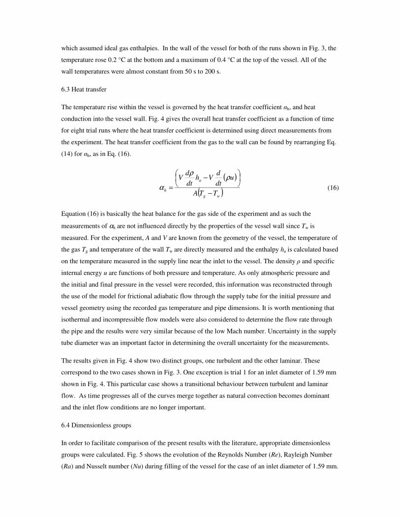
6.3 Heat transfer
The temperature rise within the vessel is governed by the heat transfer coefficient αh, and heat
conduction into the vessel wall. Fig. 4 gives the overall heat transfer coefficient as a function of time
for eight trial runs where the heat transfer coefficient is determined using direct measurements from
the experiment. The heat transfer coefficient from the gas to the wall can be found by rearranging Eq.
(14) for αh, as in Eq. (16).
( )
( )wg
a
hTTA
udt
dVh
dt
dV
−
−
=
ρρ
α (16)
Equation (16) is basically the heat balance for the gas side of the experiment and as such the
measurements of αh are not influenced directly by the properties of the vessel wall since Tw is
measured. For the experiment, A and V are known from the geometry of the vessel, the temperature of
the gas Tg and temperature of the wall Tw are directly measured and the enthalpy ha is calculated based
on the temperature measured in the supply line near the inlet to the vessel. The density ρ and specific
internal energy u are functions of both pressure and temperature. As only atmospheric pressure and
the initial and final pressure in the vessel were recorded, this information was reconstructed through
the use of the model for frictional adiabatic flow through the supply tube for the initial pressure and
vessel geometry using the recorded gas temperature and pipe dimensions. It is worth mentioning that
isothermal and incompressible flow models were also considered to determine the flow rate through
the pipe and the results were very similar because of the low Mach number. Uncertainty in the supply
tube diameter was an important factor in determining the overall uncertainty for the measurements.
The results given in Fig. 4 show two distinct groups, one turbulent and the other laminar. These
correspond to the two cases shown in Fig. 3. One exception is trial 1 for an inlet diameter of 1.59 mm
shown in Fig. 4. This particular case shows a transitional behaviour between turbulent and laminar
flow. As time progresses all of the curves merge together as natural convection becomes dominant
and the inlet flow conditions are no longer important.
6.4 Dimensionless groups
In order to facilitate comparison of the present results with the literature, appropriate dimensionless
groups were calculated. Fig. 5 shows the evolution of the Reynolds Number (Re), Rayleigh Number
(Ra) and Nusselt number (Nu) during filling of the vessel for the case of an inlet diameter of 1.59 mm.

The Reynolds numbers lower than 2000 show that the flow in the inlet pipe was laminar. As
mentioned earlier, the flow inside the vessel however was probably initially turbulent based on the
temperature fluctuations observed in Fig. 3(a). This shows that a laminar flow model is suitable for
the pipe but a turbulence model may be required for computational fluid dynamics simulations of the
flow field in the vessel even at the present low-Reynolds number conditions. The falling Reynolds
number indicates that forced convection heat transfer will decrease as the vessel fills. On the other
hand, the Rayleigh number has a peak at around 50 s indicating that the driving forces for natural
convection become more important as time progresses and then eventually decrease as the filling is
completed.
The measured Reynolds numbers and Rayleigh numbers individually fall within the range specified
by Woodfield et al [18] from time 20 s to 60 s. However, combining the two using Eq. (11) yields
Nusselt numbers that are mostly smaller than all of data reported by Woodfield et al [18]. Moreover,
the correlation given by Eq. (11) was developed using a single vessel with dimensionless geometry
ratios d/D = 0.14 and H/D = 2.8 whereas in the present experiment d/D = 0.021 or 0.07 and H/D =
2.6. Therefore it is clear that the present study corresponds to a region of data not previously
investigated by the authors. Fig. 5 also gives a comparison between the measured Nusselt number and
that calculated using Eq. (11). There are some notable differences. Apart from the first 10 seconds, the
Nusselt number is over-predicted by the correlation. Also the shape of the predicted curve is notably
different to the measurements during the early stages of filling. This highlights a weakness in either
the model or in the heat transfer coefficient correlation.
Fig. 6(a) shows the measured Nusselt numbers against predictions using Eq. (11) for the eight
experimental runs shown previously in Fig. 4. For the purpose of comparison, data from Ref. [18] are
also included in the figure. It is clear from this figure that the present data correspond to a lower
region of Nusselt number and that in spite of being an extrapolation, Eq. (11) generally gives the
correct order of magnitude for Nu. The effect of changing the value of d/D however, appears to be
exaggerated by the correlation. This is clear from a comparison of the differences between the
triangle and square symbols in Fig. 6(a). As a percentage of the magnitude of the heat transfer
coefficient, these differences appear to be relatively larger in Fig. 6(a) than in Fig. 4 comparing the
laminar and turbulent flow regimes.
Equation (11) does not consider the ratio d/D or dimensionless time. Because of the low pressure, the
thermal diffusivity of the air in the present experiment is very high. As a result, Fourier numbers are
significantly higher than those of high-pressure gas experiments. Therefore, transient heat conduction
may be an important mechanism for heat transfer in the present data. With this in mind, several
attempts were made to modify the correlation using d/D and the Fourier number τ based on the radius
of the cylinder to better capture the trends in the data. Only a marginal improvement could be made

without considering dimensionless time (τ). The following equation improves the correlation of the
present data considerably.
( ) ( ) 352.067.045.012 104.0Re38.005.151.0 RaDdNu ++−=−
ττ (17)
Equation (17) is basically a modification of Eq. (11) in that the coefficient of the Reynolds number
term is replaced by a function involving the dimensionless diameter and the Fourier number. Fig. 6(b)
compares Eq. (17) with the measured Nusselt numbers. The data from Ref. [18] are also included in
the figure. The improvement to correlating the present data leads to a slightly poorer correlation of the
data by Woodfield et al. [18] in the vicinity of Nu = 100. Equation (17) is most suitable for τ < 1.5, for
0.021 < d/D < 0.14 and for Nu < 100.
7. Conclusions
The following may be concluded from this study:
1. For low Reynolds number flow conditions, a switch from a laminar to a turbulent flow regime
was observed as a result of reducing the inlet diameter to the vessel while maintaining a
similar filling rate.
2. The thermal field for laminar flow conditions was stratified with a considerably higher peak
gas temperature (at the top of the vessel) than what was observed under turbulent flow
conditions.
3. The present experimental data was used to expand and modify the heat transfer correlation
previously developed by two of the authors [18] for filling pressure vessels to capture a wider
range of dimensionless groups than is presently available in the literature.
4. Both forced and natural convection were present in the experiment and consequently the flow
regime inside the vessel is best described as mixed convection.
References
[1] S. Maus, J. Hapke, C. N. Ranong, E. Wuchner, G. Friedlmeir, D. Wenger, Filling procedure for
vehicles with compressed hydrogen tanks, Int. J. Hydrogen Energy 33 (2008) 2513-2519.
[2] M. Monde, P. L. Woodfield, T. Takano, M. Kosaka, Estimation of temperature change in practical
hydrogen pressure tanks being filled at high pressures of 35 and 70 MPa, Int. J. Hydrogen Energy 37
(2012) 5723-5734.
[3] C. J. B. Dicken, W. Merida Modelling the transient temperature distribution within a hydrogen
cylinder during refuelling, J. Numer. Heat Transfer Part A 53 (2008) 1-24.

[4] A. Suryan, H. D. Kim, T. Setoguchi, Three dimensional numerical computations on the fast filling
of a hydrogen tank under different conditions, Int. J. Hydrogen Energy 37 (2012) 7600-7611.
[5] Y. Zhao, G. Liu, Y. Liu, J. Zheng, Y. Chen, L. Zhao, J. Guo, Y. He, Numerical study on fast
filling of 70 MPa type III cylinder for hydrogen vehicle, Int. J. Hydrogen Energy 37 (2012) 17517-
17522.
[6] M. Heitsch, D. Baraldi, P. Moretto, Numerical Investigations on the fast filling of hydrogen tanks,
Int. J. Hydrogen Energy 36 (2011) 2606-2612.
[7] C. J. B. Dicken, W. Merida, Measured effects of filling time and initial mass on the temperature
distribution within a hydrogen cylinder during refuelling. J Power Sources 165 (2007) 324-36.
[8] P. L. Woodfield, M. Monde, Y. Mitsutake, Heat transfer characteristics for practical hydrogen
pressure vessels being filled at high pressure, J. Thermal Sci. Tech. 2 (2008) 241-253.
[9] S. Charton, V. Blet, J. P. Corriou, A simplified model for real gas expansion between two
reservoirs connected by a thin tube, Chem. Eng. Sci. 51 (1996) 295-308.
[10] J. Xiao, J. R. Travis, W. Breitung, Hydrogen release from a high pressure gaseous hydrogen
reservoir in case of a small leak, Int. J. Hydrogen Energy 36 (2011) 2545-2554.
[11] L. Cardinali, S. Santomassimo, M. Stefanoni, Design and realization of a 300 W fuel cell
generator on an electric bicycle, J. Power Sources 106 (2002) 384-387.
[12] K. Haraldsson, A. Folkesson, P. Alvfors, Fuel cell busses in the Stockholm CUTE project – First
experiences from a climate perspective, J. Power Sources 145 (2005) 620-631.
[13] J. J. Hwang, Review on development and demonstration of hydrogen fuel cell scooters,
Renewable Sustainable Energy Reviews 16 (2012) 3803-3815.
[14] W.S. Winters, G.H. Evans, S.F. Rice, R. Greif, An experimental and theoretical study of heat and
mass transfer during the venting of gas from pressure vessels, Int. J. Heat Mass Transfer 55 (2012) 8-
18.
[15] S. Paolucci, Heat transfer during the early expansion of gas in pressurized vessels, Int. J. Heat
Mass Transfer 28 (1985) 1525-1537.
[16] D. E. Daney, Turbulent natural convection of liquid deuterium, hydrogen and nitrogen within
enclosed vessels, Int. J. Heat Mass Transfer 19 (1976) 431-441.

[17] L. B. Evans, N. E. Stefany, An experimental study of transient heat transfer to liquids in
cylindrical enclosures, Chemical Engineering Progress Symposium Series, American Institute of
Chemical Engineers 62 (1966) 209-215.
[18] P. L. Woodfield, M. Monde, Y. Mitsutake, Measurement of averaged heat transfer coefficients
in high-pressure vessel during charging with hydrogen, nitrogen or argon gas, J. Thermal Sci. Tech. 2
(2007) 180-191.
[19] F. C. Shen, Filament wound structure technology overview, Mater. Chem. Phys. 42 (1995) 96-
100.
[20] R. Fox, A. McDonald, Introduction to Fluid Mechanics, John Wiley & Sons, New York, 1992.
[21] T. V. Patankar, K. C. Karki, K. M. Kelkar, in ‘Handbook of Fluid Dynamics’, ed. by R. W.
Johnson, CRC Press, Boca Raton USA, 1998.
[22] R. J. Moffat, Describing the uncertainties in experimental results, Exper. Therm. Fluid Sci. 1
(1988) 3-17.

Fig. 1 CFRP vessel construction, geometry and thermocouple positions
G7
G8
Air Inlet
G5
G6 G3
G4
G1
G2
Inside Diameter 70 mm
180 mm
15
50
50
50
Thermocouple hot junctions 20
Inlet diameter adjustable
depending on selected insert
CFRP Wall thickness: 4 mm
Thermocouple wires
glued to flange and
sandwiched between
two half-cylinders
Thermocouples embedded in wall
during manufacture of composite
Germanium window

Fig. 2 Experimental setup
Thermal camera
Pressure vessel
Supply tube
Thermocouple
wires
Thermally
transparent
window
Valve 1
Vacuum
pump Vacuum pressure
meter
Valve 2
Digital
multimeter/ P.C.
Air in

Fig. 3 Measured temperatures during filling of the vessel. The locations of the thermocouples are
illustrated in Fig. 1
Ma
ss
flo
wra
te(m
g/s
)
Pre
ss
ure
(kP
a)
-5
0
5
10
15
20
25
0
20
40
60
80
100
Time (s)
Te
mp
era
ture
(°C
)
0 50 100 150 20020
21
22
23
24
25
26
27
28
29
30
31
32
Wall
Supply Temperature
G1
G3
G2G4
G5
G8
G6
G7
Inlet Temperature
(a) 1.59 mm inlet diameter
Pressure
MassFlowrate
Ma
ss
flo
wra
te(m
g/s
)
Pre
ss
ure
(kP
a)
-5
0
5
10
15
20
25
0
20
40
60
80
100
Time (s)T
em
pe
ratu
re(°
C)
0 50 100 150 20020
21
22
23
24
25
26
27
28
29
30
31
32
Wall Temperatures
Supply Temperature
G1
G3
G2
G4
G5G8
G6
G7
Inlet Temperature
(b) 5.25 mm inlet diameter
Pressure
Mass Flowrate
Fig. 4 Measured heat transfer coefficients during filling the vessel.
Time (s)
αh
(W/(
m2K
))
100
101
102
0
2
4
6
8
10
12
1.59 mm inlet, trial 11.59 mm inlet, trial 21.59 mm inlet, trial 31.59 mm inlet, trial 4
1.59 mm inlet, trial 55.25 mm inlet, trial 15.25 mm inlet, trial 25.25 mm inlet, trial 3
Turbulent
Laminar flow behaviour
Naturalconvection

Fig. 5 Measured dimensionless groups
Time (s)
Re
yn
old
sN
um
be
r
Ra
yle
igh
Nu
mb
er
Nu
ss
elt
Nu
mb
er
0 50 100 150 2000
200
400
600
800
0
200000
400000
600000
800000
1E+06
1.2E+06
1.4E+06
0
50
100
150
Reynolds NumberRayleigh NumberNusselt Number0.56Re
0.67+0.104Ra
0.352
Ra
Re
Nu
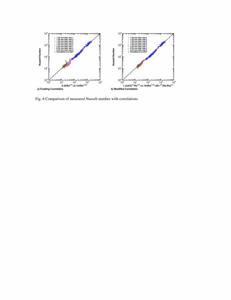
Fig. 6 Comparison of measured Nusselt number with correlations
0.56Re0.67
+0.104Ra0.352
Nu
sse
ltN
um
be
r
100
101
102
103
104
100
101
102
103
104
a) Existing Correlation
1.59 mm inlet, trial 11.59 mm inlet, trial 21.59 mm inlet, trial 31.59 mm inlet, trial 41.59 mm inlet, trial 55.25 mm inlet, trial 15.25 mm inlet, trial 25.25 mm inlet, trial 3Woodfield et al 2007
1.5(d/D)0.5
Re0.67
+0.104Ra0.352
+80τ-0.5
(Re/Ra)0.3
Nu
sse
ltN
um
be
r
100
101
102
103
104
100
101
102
103
104
b) Modified Correlation
1.59 mm inlet, trial 11.59 mm inlet, trial 21.59 mm inlet, trial 31.59 mm inlet, trial 41.59 mm inlet, trial 55.25 mm inlet, trial 15.25 mm inlet, trial 25.25 mm inlet, trial 3Woodfield et al 2007