an experimental survey of mapreduce-based …ynsilva/simcloud/downloads/simjoin...an experimental...
TRANSCRIPT

An Experimental Survey of MapReduce-based Similarity Joins, p. 1, 2016.
© Springer-Verlag Berlin Heidelberg 2016
An Experimental Survey of MapReduce-based Similarity
Joins*
Yasin N. Silva, Jason Reed, Kyle Brown, Adelbert Wadsworth, Chuitian Rong
Arizona State University
{ysilva, jmreed3, kabrow17, ajwadswo, crong5}@asu.edu
Abstract. In recent years, Big Data systems and their main data processing
framework - MapReduce, have been introduced to efficiently process and analyze
massive amounts of data. One of the key data processing and analysis operations
is the Similarity Join (SJ), which finds similar pairs of objects between two da-
tasets. The study of SJ techniques for Big Data systems has emerged as a key
topic in the database community and several research teams have published tech-
niques to solve the SJ problem on Big Data systems. However, many of these
techniques were not experimentally compared against alternative approaches.
This was the case in part because some of these techniques were developed in
parallel while others were not implemented even as part of their original publi-
cations. Consequently, there is not a clear understanding of how these techniques
compare to each other and which technique to use in specific scenarios. This pa-
per addresses this problem by focusing on the study, classification and compari-
son of previously proposed MapReduce-based SJ algorithms. The contributions
of this paper include the classification of SJs based on the supported data types
and distance functions, and an extensive set of experimental results. Furthermore,
the authors have made available their open-source implementation of many SJ
algorithms to enable other researchers and practitioners to apply and extend these
algorithms.
Keywords: Similarity Joins, Big Data Systems, Performance Evaluation,
MapReduce.
1 Introduction
The processing and analysis of massive amounts of data is a crucial requirement in
many commercial and scientific applications. Internet companies, for instance, collect
large amounts of data such as content produced by web crawlers, service logs and click
streams generated by web services. Analyzing these datasets may require processing
tens or hundreds of terabytes of data. Big Data systems and MapReduce, their main
data processing framework, constitute an answer to the requirements of processing mas-
sive datasets in a highly scalable and distributed fashion. These systems are composed
* This work was supported by Arizona State University’s SRCA and NCUIRE awards, the
NSFC (No.61402329), and the China Scholarship Council.

of large clusters of commodity machines and are often dynamically scalable, i.e., cluster
nodes can easily be added or removed depending on the workload. Important examples
of these Big Data systems are: Apache Hadoop [26]; Google’s File System [10],
MapReduce [9] and Bigtable [8]; and Microsoft’s Dryad [11] and SCOPE/Cosmos [7].
The Similarity Join is one of the most useful operations for data processing and
analysis. This operation retrieves all data pairs from two datasets (R and S) whose dis-
tances are smaller than or equal to a predefined threshold ε. Similarity Joins have been
extensively used in domains like record linkage, data cleaning, sensor networks, mar-
keting analysis, multimedia applications, recommendation systems, etc. A significant
amount of work has been focused on the study of non-distributed implementations.
Particularly, Similarity Joins have been studied as standalone operations [12, 13, 14,
15, 30], as operations that use standard database operators [16, 17, 18], and as physical
database operators [1, 2, 3, 4, 5, 29, 31].
The study of Similarity Join techniques for Big Data systems has recently emerged
as a key topic in the data management systems community. Several research teams have
proposed and published different techniques to solve the Similarity Join problem on
Big Data systems (e.g., [19, 20, 21, 22, 23, 24, 25]). Unfortunately, however, many of
these techniques were not experimentally compared against alternative approaches.
This was the case in part because some of these techniques were developed in parallel
while others were not implemented even as part of their original publications. Conse-
quently, while there are many techniques to solve the Similarity Join problem, there is
not a clear understanding of: (1) how these techniques compare to each other, and (2)
which technique to use in real-world scenarios with specific requirements for data
types, distance functions, dataset sizes, etc. Furthermore, the need for comparative work
in the area of data management was recently highlighted by the editors of a top journal
in this area [6].
This paper addresses this problem by focusing on the study, classification and com-
parison of the Similarity Join techniques proposed for Big Data systems (using the
MapReduce framework). The main contributions of this paper are:
The classification of Similarity Join techniques based on the supported data types
and distance functions.
An extensive set of experimental results. These results include tests that compare the
performance of alternative approaches (based on supported data type and distance
function) under various dataset sizes and distance thresholds.
The availability of the authors’ open-source implementation of many Similarity Join
algorithms [27]. Our goal is to enable other researchers and practitioners to apply
and extend these algorithms.
The remaining part of this paper is organized as follows. Section 2 presents the de-
scription of all the algorithms considered in our study and a classification of the algo-
rithms based on the supported data types and distance functions. Section 3 presents the
experimental evaluation results and discussions (this section is divided into subsections
that focus on specific data types and distance functions). Finally, Section 4 presents the
conclusions.

2 MapReduce-based Similarity Join Algorithms
2.1 Classification of the Algorithms
Table 1 presents the MapReduce-based Similarity Join algorithms considered in our
study. For each algorithm, the table shows the supported data types and distance func-
tions (DFs), and the data types that could be supported by extending the original algo-
rithms. In order to systematically evaluate the different algorithms, we classify them
based on the supported data types. The experimental section of this paper, compares all
the algorithms that support a given data type and its associated distance functions.
Table 1. Similarity Join algorithms and supported distance functions and data types.
2.2 Description of the Studied Similarity-Join Algorithms
Naïve Join. The Naïve Join algorithm [22] is compatible with all data types and dis-
tance functions, and works in a single MapReduce job. The algorithm uses a key space
defined by a parameter J, which is proportional to the square root of the number of
reducers (reduce tasks) to be used. During the Map phase, pairs of input data elements
are assigned to a key pair with the form (i, j) where 0 ≤ 𝑖 ≤ 𝑗 ≤ 𝐽. For each input record
X, the mapper (map task) outputs key-value pairs with the form ((i, j), X), such that any
two records are mapped to at least one common key. The reducer receives all of the
Algorithm Supported Distance/
Similarity Functions
Supported Data Types
Text/String Numeric Vector Set
Naïve Join Any DF ● ● * ●
Ball Hashing 1 Hamming Distance
Edit Distance
●
Ball Hashing 2 Hamming Distance
Edit Distance
●
Subsequence Edit Distance ●
Splitting Hamming Distance
Edit Distance
●
Hamming Code Hamming Distance ●
Anchor Points Hamming Distance
Edit Distance
● * *
MRThetaJoin Any DF ● ● ● ●
MRSimJoin Any metric DF ● ● ● ●
MRSetJoin JS, TC, CC,
Edit Distance*
* ●
Online Aggregation JS, RS, DS, SC, VC ●
Lookup JS, RS, DS, SC, VC ●
Sharding JS, RS, DS, SC, VC ●
● Natively Supported
* Can be extended to support this data type or distance function
JS=Jaccard Similarity, TC=Tanimoto Coefficient, CC=Cosine Coefficient, RS=Ruzicka Sim-
ilarity, DS=Dice Similarity, SC=Set Cosine Sim., VC=Vector Cosine Sim.

records for a given key and compares each pair of records outputting the pairs with
distance smaller than or equal to ε (distance threshold). The algorithm proposed in [22]
does not consider the case where two records are mapped to more than one common
key. In this case, we solved the problem by outputting only when i=j.
Ball Hashing 1. The Ball Hashing 1 algorithm [22] takes a brute force approach to
solving the Similarity Join problem. This algorithm assumes that the alphabet of the
input value is finite and known. The Map phase takes in a given input record r and
generates a ball of radius ε. In effect, for a given join attribute vr, it will generate a set
Vr composed of every possible value within ε of vr. For each value Vri in Vr that is not
equal to vr, the Map will emit the key-value pair < Vri, r>. The Map will additionally
output the key-value pair <vr, r>. As vr is the join attribute in r, this ensures a collision
in the Reduce phase with any matching pairs (links). Any Reduce group that contains
such a record (<vr, r>) should be considered an active group and the record r should be
considered native to that group. Any Reduce group that does not have a native record
within it should be considered inactive and does not need to be processed further. In the
active groups, the join matches are generated by combining the native members with
each of the non-native members in the group. The original paper does not consider the
possibility of multiple input records having the same join value. If this is the case, there
is the additional need to join native members among each other as well as all native
records against all non-native records. This algorithm supports string data with the Edit
and Hamming distance functions.
Ball Hashing 2. Ball Hashing 2 [22] is an extension of the Ball Hashing 1 algorithm.
The difference is that in the Map phase, it generates balls of size ε/2. Because of this, it
is necessary to process every Reduce group. A brute force comparison is performed in
each Reduce group to find any matches and eliminate the possibility of duplicate out-
puts. The algorithm supports string data with Edit and Hamming distance metrics.
Subsequence. Subsequence [22] is an algorithm proposed for string data and the Edit
Distance. The Map phase generates all the (b-ε/2)-subsequences of each input string (b
is the string length) and outputs pairs of the form <subsequence, input_string>. The
Reduce phase compares all the records sharing the same subsequence to identify the
Similarity Join matches. The key idea behind this algorithm is that if two strings are
within ε, they will share at least one identical subsequence.
Splitting. The Splitting algorithm [22] is composed of a single MapReduce job and is
based on splitting strings into substrings. These substrings are then compared to other
substrings generated from the input dataset. In order to be considered a Similarity Join
match, a pair of strings only needs to share one common substring. In the Map task,
each input string (with length b) is split into substrings of length b/(ε+1). The result
will be composed of b/(b/(ε+1)) substrings. Each substring will be outputted with a key
consisting of its position (i) in the parent string, and the substring that was generated,

si. The value that will be attached to the key is the parent string. Each reducer will
compare (pair wise) all the substrings that have a matching key and output the pairs that
are separated by a distance smaller than or equal to ε. To avoid the generation of dupli-
cate pairs at multiple reducers, a match is generated only within the Reduce group as-
sociated with the position of the first common substring between two matching strings.
This distance functions supported by this algorithm are Hamming and Edit Distance.
Anchor Points. This algorithm distributes the input data into groups where all the
members of a group are within a certain distance of an anchor point [22]. The technique
supports the Hamming and Edit Distance functions. In the case of Hamming Distance,
the algorithm finds first a set of anchor points such that every input record is within ε
from at least one anchor. This set is stored in a distributed cache and used at each map-
per. For each input record s, the mapper outputs key-value pairs for every anchor point
that is within 2ε of s. The mapper marks the closest anchor point to s as its home group.
In the Reduce phase, the strings of a given home group will be compared to other strings
from other groups that were sent to the same reducer. All strings in the home group will
be compared as well. In the case of Edit Distance, the anchor points are a subset of the
data such that every input record is within ε deletions from at least one anchor. This
modified algorithm only works with fixed-length strings. This fact is not directly stated
in the paper but was confirmed by the authors.
Hamming Code. The Hamming Code algorithm [22] is a SJ technique proposed for
string data and the Hamming Distance. Since this algorithm only works when ε=1 and
the strings’ length is one less than a power of 2, it is not included in our evaluation.
MRThetaJoin. MRThetaJoin [23] is a randomized Theta Join algorithm that supports
arbitrary join predicates (including Similarity Join conditions). This approach uses a
single MapReduce job and requires some basic statistics (input cardinality). The ap-
proach uses a model that partitions the input relations using a matrix that considers all
the combinations of records that would be required to answer a cross product. The ma-
trix cells are then assigned to reducers in a way that minimizes job completion time. A
memory-aware variant is also proposed for the common scenario where partitions do
not fit in memory. Since any Theta Join or Similarity Join is a subset of the cross-
product, the matrix used in this approach can represent any join condition. Thus, this
approach can be used to supports Similarity Joins with any distance function and data
type. For the performance evaluation of Similarity Joins presented in this paper, we
implemented an adaptation of the memory-aware 1-Bucket-Theta algorithm proposed
in [25] that uses the single-node QuickJoin algorithm [15] in the reduce function.
MRSimJoin. The MRSimJoin algorithm [20, 21, 32] iteratively partitions the data into
smaller partitions, until each partition is small enough to be processed in a single node.
The process is divided into a sequence of rounds, and each round corresponds to a
MapReduce job. Partitioning is achieved by using a set of pivots, which are a subset of

the records to be partitioned. There are two types of partitions, base partitions and
window-pair partitions. Base partitions hold all of the records closest to a given pivot,
rather than any other pivot. Window-pair partitions hold records within the boundary
between two base partitions. If possible, e.g., Euclidean Distance, the window-pair par-
titions should only include the points within ε from the hyperplane separating adjacent
base partitions. If this is not possible, a distance is computed to a generalized hyper-
plane boundary (lower bound of the distance). This algorithm can be used with any data
type and metric. The experimental section in [20] shows that in most cases the number
of pivots can be adjusted to ensure the algorithm runs in a single MapReduce job.
MRSetJoin. MapReduce Set-Similarity Join [19] is a Similarity Join algorithm that
consists of three stages made up of various MapReduce jobs. In the first stage, data
statistics are generated in order to select good signatures, or tokens, that will be used
by later MapReduce jobs. In the second stage, each record has its record-ID and join-
attribute value assigned to the previously generated tokens, the similarity between rec-
ords associated with the same token is computed, and record-ID pairs of similar records
are outputted. In the third stage, pairs of joined records are generated from the output
of the second stage and the original input data. MRSetJoin supports set-based distance
functions like Jaccard Distance and Cosine Coefficient. There are multiple options pre-
sented for each stage, however, the paper states that BTO-PK-BRJ is the most robust
and reliable option. Thus, this option is used in this survey as the representative of this
technique.
V-Smart-Online Aggregation. Online Aggregation [24] is a Similarity Join algorithm
under the V-SMART-Join framework, which can be used for set and multiset data and
set-based distance functions like Jaccard and Dice. In general, the V-SMART-Join
framework consists of two phases, joining and similarity. Although the framework in-
cludes three different joining phase algorithms, Online Aggregation, Lookup, and Shar-
ding, only one of the three was selected to participate in the survey. According to the
experimental results in [24], Online Aggregation generally outperforms the Sharding
and Lookup algorithms, and as such it was selected to represent this approach. The
algorithm is based on the computation of Uni(Mi) for each multiset Mi. Uni(Mi) is the
partial result of a unilateral function (e.g., Uni(Mi)=|Mi|). During the joining phase (one
MapReduce job), the Uni(Mi) of a given multiset Mi is joined to all the elements of Mi.
The similarity phase, composed of two MapReduce jobs, builds an inverted index, com-
putes the similarity between all candidate pairs, and outputs the Similarity Join matches.
3 Experimental Comparison
This section presents the experimental comparison of previously proposed MapReduce-
based Similarity Join algorithms. One of the key tasks for this survey work was the
implementation of the studied algorithms. While in some cases, the source code was
provided by the original authors (MRSetJoin, MRSimJoin), in most cases, the source

code was not available and consequently had to be implemented as part of our work
(e.g., Ball Hashing 1, Ball Hashing 2, Naïve Join, Splitting, Online Aggregation,
MRThetaJoin). We have made available the source code of all the evaluated algorithms
in [27]. All the algorithms were implemented and evaluated using Hadoop (0.20.2), the
most popular open-source MapReduce framework. The experiments were performed
using a Hadoop cluster running on the Amazon Elastic Compute Cloud (EC2). Unless
otherwise stated, we used a cluster of 10 nodes (1 master + 9 worker nodes) with the
following specifications: 15 GB of memory, 4 virtual cores with 2 EC2 Compute Units
each, 1,690 GB of local instance storage, 64-bit platform. The number of reducers was
computed as: 0.95×⟨no. worker nodes⟩×⟨max reduce tasks per node⟩ = 25. Table 2
shows configurations details for individual algorithms.
The experiments used a slightly modified version of the Harvard bibliographic da-
taset [28]. Specifically, we used a subset of the original dataset and augmented the rec-
ord structure with a vector attribute to perform the tests with vector data. Each record
contains the following attributes: unique ID, title, date issued, record change date, rec-
ord creation date, Harvard record-ID, first author, all author names, and vector. The
vector attribute is a 10D vector that was generated based on the characters of the title
(multiplied against prime numbers). The vector components are in the range [0 - 999].
The minimum and maximum length (number of characters) of each attribute are as fol-
lows: unique ID (9, 9), title (6, 996), date issued (4, 4), record change date (15, 15),
record creation date (6, 6), Harvard record-ID (10, 10), first author (6, 94), and all au-
thor names (6, 2462). The dataset for scale factor 1 (SF1) contains 200K records. The
records of each dataset are equally divided between tables R and S.
The datasets for SF greater than 1 were generated in such a way that the number of
matches of any Similarity Join operation in SFN is N times the number of matches in
SF1. For vector data, the datasets for higher SF were obtained adding shifted copies of
the SF1 dataset where the distance between copies were greater than the maximum
value of ε. For string data, the datasets for higher SF were obtained adding a copy of
the SF1 data where characters are shifted similarly to the process in [19].
We evaluate the performance of the algorithms by independently analyzing their ex-
ecution time while increasing the dataset size (SF) and the distance threshold (ε). We
did not include the execution time when an algorithms took a relatively long time (more
than 3 hours). We performed four sets of experiments for the following combinations
of data types and distance functions: (1) vector data and Euclidean Distance, (2) varia-
ble-length string (text) data and Edit Distance, (3) fixed-length string data and Ham-
ming Distance, and (4) set data and Jaccard Distance. Each algorithm was executed
multiple times; we report the average execution times.
Table 2. Additional configuration details.
Algorithm Configuration Details
Naïve Join J = √Number of Reduce Tasks
MRThetaJoin K = ((|R|+|S|) x b)/m, where |R| and |S| are the cardinalities of R and
S, b = size in bytes per record, m = memory threshold (64 MB).
MRSimJoin Memory limit for in-memory SJ algorithm = 64 MB.
Number of Pivots = SF x 100.

3.1 Comparison of Algorithms for Vector Data – Euclidean Distance
This section compares the performance of the algorithms that support vector data,
namely MRSimJoin and MRThetaJoin. We use the Euclidean Distance function and
perform the distance computations over the 10D vector attribute of the Harvard dataset.
Increasing Scale factor. Figures 1 and 2 compare the way MRSimJoin and MRThe-
taJoin scale when the data size increases (SF1-SF4). The experiments use 10D vectors.
The experiments in Fig. 1 use a relatively small value of ε (5% of the maximum possible
distance) while the ones in Fig. 2 a relatively large value (15%). Fig. 1 shows that, for
small values of ε (5%), MRSimJoin performs significantly better than MRThetaJoin
when the data size increases. Specifically, the execution time of MRThetaJoin grows
from being 2 times the one of MRSimJoin for SF1 to 7 times for SF4. The execution
time of MRThetaJoin is significantly higher than that of MRSimJoin because the total
size of all the partitions of MRThetaJoin is significantly larger than that of MRSimJoin.
Fig. 2 shows that, for larger values of ε (15%), MRSimJoin still performs better than
MRThetaJoin in the case of larger datasets but is outperformed by MRThetaJoin for
small datasets. Specifically, the execution time of MRThetaJoin is 0.7 times the one of
MRSimJoin for SF1 and SF2; and 1.2 and 1.9 times for SF3 and SF4, respectively.
Increasing ε. Figures 3 and 4 show how the execution time of MRSimJoin and MRThe-
taJoin increase when ε increases (1%-20%). Fig. 3 considers relatively smaller values
of ε (1%-5%) while Fig. 4 considers larger values (5%-20%). The results in both figures
show that the performance of MRSimJoin is better than the one of MRThetaJoin for all
the evaluated values of ε. Specifically, in Fig. 3 the execution time of MRThetaJoin is
between 7 (ε=5%) to 11 (ε=1%) times the one of MRSimJoin while in Fig. 4, the exe-
cution time of MRThetaJoin is between 1.6 (ε=20%) to 9.2 (ε=5%) times the one of
MRSimJoin. We can observe that the performance of MRSimJoin tends to get closer to
the one of MRThetaJoin for very large values of ε. In general, the execution time of
both algorithms grows when ε grows. The increase in execution time is due to a higher
number of distance computations in both algorithms and slightly larger sizes of win-
dow-pair partitions in the case of MRSimJoin.
From the results presented in this section, we can conclude that MRSimJoin is in
general the best approach to perform Similarity Joins with vector data unless the dataset
size is very small and the distance threshold is extremely large.
3.2 Comparison of Algorithms for Variable-length String Data – Edit Distance
This section compares the performance of the Similarity Join algorithms using string
data and the Edit Distance. The tests use the first author name (variable-length: 6-94,
alphabet size: 27) as the join attribute. The evaluated algorithms are: MRSimJoin, Na-
ïve Join, MRThetaJoin, and Ball Hashing 1. For this last algorithm, we were only able
to obtain results for the test with ε=1. Even using SF1, this algorithm took significantly
longer than the other algorithms. Ball Hashing 2 and Anchor Points are not included
since they do not support variable-length strings. Splitting and Subsequence were not
included since the brief information included in [22] to support variable-length strings
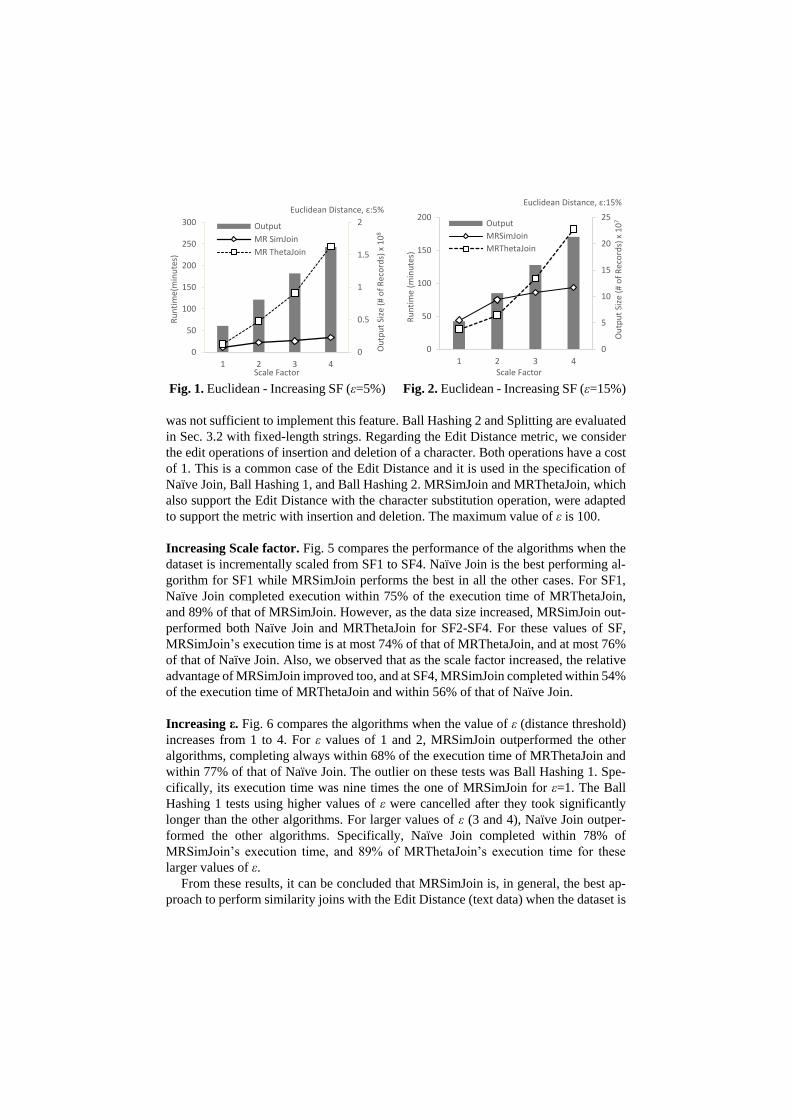
Fig. 1. Euclidean - Increasing SF (ε=5%) Fig. 2. Euclidean - Increasing SF (ε=15%)
was not sufficient to implement this feature. Ball Hashing 2 and Splitting are evaluated
in Sec. 3.2 with fixed-length strings. Regarding the Edit Distance metric, we consider
the edit operations of insertion and deletion of a character. Both operations have a cost
of 1. This is a common case of the Edit Distance and it is used in the specification of
Naïve Join, Ball Hashing 1, and Ball Hashing 2. MRSimJoin and MRThetaJoin, which
also support the Edit Distance with the character substitution operation, were adapted
to support the metric with insertion and deletion. The maximum value of ε is 100.
Increasing Scale factor. Fig. 5 compares the performance of the algorithms when the
dataset is incrementally scaled from SF1 to SF4. Naïve Join is the best performing al-
gorithm for SF1 while MRSimJoin performs the best in all the other cases. For SF1,
Naïve Join completed execution within 75% of the execution time of MRThetaJoin,
and 89% of that of MRSimJoin. However, as the data size increased, MRSimJoin out-
performed both Naïve Join and MRThetaJoin for SF2-SF4. For these values of SF,
MRSimJoin’s execution time is at most 74% of that of MRThetaJoin, and at most 76%
of that of Naïve Join. Also, we observed that as the scale factor increased, the relative
advantage of MRSimJoin improved too, and at SF4, MRSimJoin completed within 54%
of the execution time of MRThetaJoin and within 56% of that of Naïve Join.
Increasing ε. Fig. 6 compares the algorithms when the value of ε (distance threshold)
increases from 1 to 4. For ε values of 1 and 2, MRSimJoin outperformed the other
algorithms, completing always within 68% of the execution time of MRThetaJoin and
within 77% of that of Naïve Join. The outlier on these tests was Ball Hashing 1. Spe-
cifically, its execution time was nine times the one of MRSimJoin for ε=1. The Ball
Hashing 1 tests using higher values of ε were cancelled after they took significantly
longer than the other algorithms. For larger values of ε (3 and 4), Naïve Join outper-
formed the other algorithms. Specifically, Naïve Join completed within 78% of
MRSimJoin’s execution time, and 89% of MRThetaJoin’s execution time for these
larger values of ε.
From these results, it can be concluded that MRSimJoin is, in general, the best ap-
proach to perform similarity joins with the Edit Distance (text data) when the dataset is
0
0.5
1
1.5
2
0
50
100
150
200
250
300
1 2 3 4
Ou
tpu
t Si
ze (
# o
f R
eco
rds)
x 1
08
Ru
nti
me(
min
ute
s)
Scale Factor
Euclidean Distance, ε:5%
Output
MR SimJoin
MR ThetaJoin
0
5
10
15
20
25
0
50
100
150
200
1 2 3 4
Ou
tpu
t Si
ze (
# o
f R
eco
rds)
x 1
07
Ru
nti
me
(min
ute
s)
Scale Factor
Euclidean Distance, ε:15%
Output
MRSimJoin
MRThetaJoin

Fig. 3. Euclidean - Increasing ε (small) Fig. 4. Euclidean - Increasing ε (large)
Fig. 5. Edit Dist. - Increasing SF Fig. 6. Edit Dist. - Increasing ε
large (greater than SF1 in our tests) or the distance threshold is relatively small (1 or 2
in our tests). For smaller datasets or larger distance thresholds, Naïve Join is the best
approach among the evaluated algorithms.
3.3 Comparison of Algorithms for Fixed-length Strings – Hamming Distance
The tests in this section perform Similarity Joins using Hamming Distance over the first
6 characters of the first author name (fixed-length: 6, alphabet: 27). The evaluated al-
gorithms are: MRSimJoin, MRThetaJoin, Naïve Join, Splitting, Ball Hashing 1, and
Ball Hashing 2. Anchor Points it is not included since the paper that introduced it
showed that it is outperformed by other algorithms [22]. The maximum value of ε is 6.
Increasing Scale Factor. The results of the experiments using increasing scale factors
(SF1-SF4) are represented in Fig. 7. This figure shows that the Splitting algorithm out-
performs all of the other algorithms for all the values of scale factor. Specifically, Split-
ting’s execution time is at most 71% of the one of MRThetaJoin, 60% of Naïve Join,
and 24% of MRSimJoin. MRThetaJoin and Naïve Join have very similar results, with
MRThetaJoin slightly outperforming Naïve Join for SF1, SF3 and SF4. The execution
0
0.5
1
1.5
2
0
50
100
150
200
250
300
1% 2% 3% 4% 5%
Ou
tpu
t Si
ze (
# o
f R
eco
rds)
x1
08
Ru
nti
me(
min
ute
s)
Distance Threshold (ε)
Euclidean Distance, SF:4
OutputMR SimJoinMR ThetaJoin
0
1
2
3
4
5
6
0
50
100
150
200
250
300
5% 10% 15% 20%
Ou
tpu
t Si
ze (
#o
f R
eco
rds)
x1
08
Ru
nti
me
(m
inu
tes)
Distance Threshold (ε)
Output
MRSimJoin
MRThetaJoin
Euclidean Distance, SF4
0
500
1000
1 2 3 4
0
5
10
Ru
nti
me
(min
ute
s)
Scale Factor
Ou
tpu
t Si
ze (
# o
f R
eco
rds)
x 1
05
Edit Distance, ε:3
Output
MRSimJoin
NaïveJoin
MRThetaJoin
0
0.5
1
1.5
2
2.5
3
3.5
1 2 3 4
0
50
100
150
200
250
300
Ou
tpu
t Si
ze (
# o
f R
eco
rds)
x 1
05
Distance Threshold (ε)
Ru
nti
me
(min
ute
s)Edit Distance, SF1Output
MRSimJoinNaïveJoinMRThetaJoinBallhashing 1

Fig. 7. Hamming Dist. - Increasing SF Fig. 8. Hamming Dist. - Increasing ε
Fig. 9. Hamming Dist. - Increasing ε (1k) Fig. 10. Jaccard - Increasing SF
time of MRSimJoin is larger than the ones of the other algorithms compared in Fig. 7.
Ball Hashing 1 and Ball Hashing 2 were excluded from the comparison as they did not
complete within a reasonable amount of time.
Increasing ε. Fig. 8 shows the results of comparing the algorithms with increasing
values of the distance threshold. In these tests, the Splitting algorithm outperforms all
other algorithms with the exception of ε=3 where MRThetaJoin slightly outperforms it.
Splitting’s execution times are between 11% (ε=1) and 106% (ε=3) of those of MRThe-
taJoin. Splitting’s execution times are also between 15% and 92% of the ones of Naïve
Join, between 3% and 90% of MRSimJoin, and less than 4% of the execution time of
Ball Hashing 1 and Ball Hashing 2. Ball Hashing 1 and 2 are not reported in Fig. 7 (and
only have some data points in Fig. 8) because they did not return a result under a sig-
nificantly long time (3 hours). Fig. 9 presents the execution time of these algorithms
with a significantly smaller dataset (1K records) under multiple values of ε. Observe
that even for this small dataset, the execution time of Ball Hashing 1 is not only signif-
icantly larger than that of Ball Hashing 2, but also increases rapidly. The execution time
of Ball Hashing 1 increases from being 2 times the execution time of Ball Hashing 2
0
100
200
300
400
500
1 2 3 4
0
2
4
6
8
Ru
nti
me
(min
ute
s)
Scale Factor
Ou
tpu
t Si
ze (
# o
f R
eco
rdS)
x 1
08
Hamming, ε:3
Output
MRSimJoin
NaïveJoin
Splitting
MRThetaJoin
0
50
100
150
200
1 2 3 4
0
2
4
6
8
Ru
nti
me
(min
ute
s)Distance Threshold (ε)
Ou
tpu
t Si
ze (
# o
f R
eco
rds)
x 1
08
Hamming, SF1OutputMRSimJoinNaïveJoinSplittingMRThetaJoinBall Hashing 1Ball Hashing 2
0
10
20
30
40
1 2 3 4
0
5
10
15
20
25
Ru
nti
me
(min
ute
s)
Distance Threshold (ε)
Ou
tpu
t Si
ze (
# o
f R
eco
rdS)
x1
03
Hamming, 1K Dataset
Output
Ball Hashing 2
Ball Hashing 1
0
200
400
1 2 3 4
0
5
10
Ru
nti
me
(min
ute
s)
Scale FactorO
utp
ut
Size
(#
of
Rec
ord
s) x
10
6
Jaccard Distance, ε:12%
OutputMRSimJoinNaïveJoinMRSetJoinMRThetaJoin

for ε=1 to be 31 times for ε=2. While Ball Hashing 2 clearly outperforms Ball Hashing
1, it is still significantly slower than other algorithms as shown in Fig. 8.
The results of this section show that in the case of Hamming Distance, the Splitting
algorithm is the best choice for various values of dataset size and distance threshold. In
most of the cases, Naïve Join and MRThetaJoin are the next best performing options.
3.4 Comparison of Algorithms for Set Data – Jaccard Distance
This section compares the performance of the algorithms that support set data, namely
Naïve Join, MRThetaJoin, MRSimJoin, MRSetJoin, and Online Aggregation. The
Lookup and Sharding algorithms were not included in our analysis since they were
found to be generally outperformed by Online Aggregation [24]. We use the Jaccard
Distance function and perform the distance computations over the First Author Name
attribute. To this end, we first converted the author name into a proper set by deleting
spaces and removing duplicates. For instance, the name “John Smith” is converted into
the set {j, o, h, n, s, m, i, t}. The alphabet size and the maximum set size are 26. In this
case, the range of ε is: 0 (0%) – 1 (100%).
Increasing Scale factor. Fig. 10 compares the way the algorithms scale when the da-
taset size increases (SF1-SF4). Naïve Join is the slowest algorithm, having a SF1
runtime that is at least four times the ones of the other algorithms in this figure. It is
also too slow to be executed with any of the higher scale factor values. MRThetaJoin
was executed with SF1 and SF2 but its runtime was too long to be included for larger
datasets. MRSimJoin and MRSetJoin have fairly similar execution times. MRSetJoin
performs better with SF1-SF3 but its relative advantage decreases as the dataset size
increases. Specifically, MRSetJoin’s execution time is 33%, 50% and 73% of those of
MRSimJoin for SF1, SF2 and SF3, respectively. MRSimJoin outperforms MRSetJoin
for SF4, where MRSimJoin’s execution time is 89% of the one of MRSetJoin. The
results of the Online Aggregation algorithm were not included because these tests took
too long and were cancelled or did not complete properly. We were able to successfully
run this algorithm only with very small datasets (~1K).
Increasing ε. Fig. 11 shows how the execution time of the evaluated algorithms in-
creases when ε increases (4%-16%). Naïve Join was the slowest algorithm and its
runtime was at least 3.5 times of the ones of the other algorithms. MRSetJoin and
MRSimJoin are the best performing algorithms. MRSetJoin’s advantage over MRSim-
Join tends to increase when ε increases. Specifically, MRSimJoin’s execution time is
1.8 times the one of MRSetJoin for SF1 and 4.7 for SF4. Fig. 12 provides additional
details of the two best performing algorithms (MRSetJoin and MRSimJoin). This figure
compares the algorithms’ performance using SF4. Fig. 12 shows that for a larger dataset
(SF4), the relative advantage of MRSetJoin over MRSimJoin decreases. In this case,
the execution time of MRSimJoin is between 0.8 and 1.8 of those of MRSetJoin.
The results presented in this section indicate that MRSetJoin is, in general, the best
algorithm for set data and Jaccard Distance. MRSimJoin, which performed second in

Fig. 11. Jaccard - Increasing ε (SF1) Fig. 12. Jaccard - Increasing ε (SF4)
most tests, should be considered as an alternative particularly for very large datasets
where it could, in fact, outperform MRSetJoin.
4 Conclusions
MapReduce is widely considered one of the key processing frameworks for Big Data
and the Similarity Join is one of the key operations for analyzing large datasets in many
application scenarios. While many MapReduce-based Similarity Join algorithms have
been proposed, many of these techniques were not experimentally compared against
alternative approaches and some of them were not even implemented as part of the
original publications. This paper aims to shed light on how the proposed algorithms
compare to each other qualitatively (supported data types and distance functions) and
quantitatively (execution time trends). The paper compares the performance of the al-
gorithms when the dataset size and the distance threshold increase. Furthermore, the
paper evaluates the algorithms under different combinations of data type (vectors,
same-length strings, variable-length strings, and sets) and distance functions (Euclidean
Distance, Hamming Distance, Edit Distance, and Jaccard Distance). One of the key
findings of our study is that the proposed algorithms vary significantly in terms of the
supported distance functions, e.g., algorithms like MRSimJoin and MRThetaJoin sup-
port multiple metrics while Subsequence and Hamming Code support only one. There
is also not a single algorithm that outperforms all the others for all the evaluated data
types and distance functions. Instead, in some cases, an algorithm performs consistently
better than the others for a given data type and metric, while in others, the identification
of the best algorithm depends on the dataset size and distance threshold. The authors
have made available the source code of all the implemented algorithms to enable other
researchers and practitioners to apply and extend these algorithms.
References
1. Y. N. Silva, W. G. Aref, M. Ali. The Similarity Join Database Operator. In ICDE, 2010.
0
200
400
4% 8% 12% 16%
0
20
40
Ru
nti
me(
min
ute
s)
Distance Threshold (ε)O
utp
ut
Size
(# o
f R
eco
rds)
x 1
05
Jaccard Distance, SF1
OutputMRSimJoinNaïveJoinMRSetJoin
0
2
4
6
8
10
0
50
100
150
200
250
300
350
4% 8% 12% 16%
Ou
tpu
t Si
ze (
# o
f R
eco
rds)
x1
06
Ru
nti
me
(min
ute
s)
Distance Threshold (ε)
Jaccard Distance, SF4
Output
MRSimJoin
MRSetJoin

2. Y. N. Silva and S. Pearson. Exploiting database similarity joins for metric spaces. In VLDB,
2012.
3. Y. N. Silva, A. M. Aly, W. G. Aref, P. -A. Larson. SimDB: A Similarity-aware Database
System. In SIGMOD, 2010.
4. Y. N. Silva, W. G. Aref, P. -A. Larson, S. Pearson, M. Ali. Similarity Queries: Their Con-
ceptual Evaluation, Transformations, and Processing. VLDB Journal, 22(3):395–420, 2013.
5. Y. N. Silva, W. G. Aref. Similarity-aware Query Processing and Optimization. VLDB PhD
Workshop, France, 2009.
6. P. A. Bernstein, C. S. Jensen, K.-L. Tan. A Call for Surveys. SIGMOD Record, 41(2): 47,
June 2012.
7. R. Chaiken, B. Jenkins, P.-A. Larson, B. Ramsey, D. Shakib, S. Weaver, and J. Zhou. Scope:
easy and efficient parallel processing of massive data sets. In VLDB, 2008.
8. F. Chang, J. Dean, S. Ghemawat, W. C. Hsieh, D. A. Wallach, M. Burrows, T. Chandra, A.
Fikes, and R. E. Gruber. Bigtable: A distributed storage system for structured data. ACM
Trans. Comput. Syst., 26(2):1–26, 2008.
9. J. Dean and S. Ghemawat. Mapreduce: simplified data processing on large clusters. In OSDI,
2004.
10. S. Ghemawat, H. Gobioff, and S.-T. Leung. The google file system. In SOSP, 2003.
11. M. Isard, M. Budiu, Y. Yu, A. Birrell, and D. Fetterly. Dryad: distributed data-parallel pro-
grams from sequential building blocks. In EuroSys, 2007.
12. V. Dohnal, C. Gennaro, and P. Zezula. Similarity Join in Metric Spaces Using eD-Index. In
DEXA, 2003.
13. C. Böhm, B. Braunmüller, F. Krebs, and H.-P. Kriegel. Epsilon Grid Order: An Algorithm
for the Similarity Join on Massive High-Dimensional Data. In SIGMOD, 2001.
14. J.-P. Dittrich and B. Seeger. GESS: a Scalable SimilarityJoin Algorithm for Mining Large
Data Sets in High Dimensional Spaces. In SIGKDD 2001.
15. E. H. Jacox and H. Samet. Metric Space Similarity Joins. TODS 33, 7:1–7:38 (2008).
16. S. Chaudhuri, V. Ganti, and R. Kaushik. A primitive operator for similarity joins in data
cleaning. In ICDE, 2006.
17. S. Chaudhuri, V. Ganti, and R. Kaushik. Data debugger: An operator-centric approach for
data quality solutions. IEEE Data Eng. Bull., 29(2):60–66, 2006.
18. L. Gravano, P. G. Ipeirotis, H. V. Jagadish, N. Koudas, S. Muthukrishnan, and D. Srivastava.
Approximate string joins in a database (almost) for free. In VLDB, 2001.
19. R. Vernica, M. J. Carey, and C. Li. 2010. Efficient Parallel Set-similarity Joins using
MapReduce. In SIGMOD, 2010.
20. Y. N. Silva, J. M. Reed, L. M. Tsosie. MapReduce-based Similarity Join for Metric Spaces.
In VLDB/Cloud-I, 2012.
21. Y. N. Silva, J. M. Reed. Exploiting MapReduce-based Similarity Joins. In SIGMOD, 2012.
22. F. N. Afrati, A. D. Sarma, D. Menestrina, A. Parameswaran, and J. D. Ullman. Fuzzy Joins
Using MapReduce. In ICDE, 2012.
23. A. Okcan and M. Riedewald. Processing Theta-joins using Mapreduce. In SIGMOD, 2011.
24. A. Metwally and C. Faloutsos. V-SMART-join: a Scalable MapReduce Framework for All-
pair Similarity Joins of Multisets and Vectors. In VLDB, 2012.
25. C. Xiao, W. Wang, X. Lin, and J. X. Yu. Efficient Similarity Joins for Near Duplicate De-
tection. In WWW, 2008.
26. Apache. Hadoop. http://hadoop.apache.org/.
27. SimCloud Project. MapReduce-based Similarity Join Survey. http://www.pub-
lic.asu.edu/~ynsilva/SimCloud/SJSurvey.
28. Harvard Library. Harvard bibliographic dataset. http://library.harvard.edu/open-metadata.

29. Y. N. Silva, S. Pearson, J. Chon, R. Roberts. Similarity Joins: Their Implementation and
Interactions with Other Database Operators. Information Systems, 52:149-162, 2015.
30. S. Pearson, Y. N. Silva. Index-based R-S Similarity Joins. In SISAP, 2014.
31. Y. N. Silva, S. Pearson, J. A. Cheney. Database Similarity Join for Metric Spaces. In SISAP,
2013.
32. Y. N. Silva, J. M. Reed, L. M. Tsosie, T. Matti. Similarity Join for Big Geographic Data. In
Geographical Information Systems: Trends and Technologies, E. Pourabbas (Ed.), pp 20-
49, CRC Press, 2014.