An Explanation of Anomalous Behavior in Models of Political Participation Jacob K. Goeree and Charles A. Holt

Abstract. This paper characterizes behavior with “noisy” decision making for models of political

interaction characterized by simultaneous binary decisions. Applications include: voting

participation games, candidate entry, the volunteer's dilemma, and collective action problems with a

contribution threshold. A simple graphical device is used to derive comparative statics and other

theoretical properties of a “quantal response” equilibrium, and the resulting predictions are

compared with Nash equilibria that arise in the limiting case of no noise. Many anomalous data

patterns in laboratory experiments based on these games can be explained in this manner.

Keywords: participation games, entry, voting, threshold public goods games, volunteer's dilemma,

quantal response equilibrium.

2

An Explanation of Anomalous Behavior in Models of Political Participation Jacob K. Goeree and Charles A. Holt*

Introduction

Many political and social decisions involve only two options: to vote or not, to enter a

contest or not, to join an alliance or not, etc. The apparent simplicity of these binary-choice

situations is somewhat misleading in that the best decision requires correct beliefs about others’

behavior. For instance, people may hesitate to go to a particular restaurant or bar when many others

are likely to go, or as Yogi Berra said, “Nobody goes there anymore. It’s too crowded.” 1 In other

cases, the rewards associated with each decision may be contingent on getting a minimal number of

decisions of a certain type, e.g. the choice by a country of whether or not to join an alliance, or jump

into world war, or impose an embargo. A similar example occurs when a majority vote is needed to

approve a legislative pay raise that each legislator would prefer not to support if it would pass

otherwise (Ordeshook 1986, chap. 3). Sometimes the minimal number of contributors needed is

only one, as in the "volunteer's dilemma," where all players are better off if at least one of them

incurs a cost from vetoing an option, attempting a dangerous rescue, or volunteering to perform a

task that benefits them all (Diekmann 1985).

In all these examples, the question is whether independent choices made by different people

will somehow generate the “correct” amount of participation or whether the inability to coordinate

will lead to deficiencies such as excess entry or crowding, insufficient effort to produce a public

good, or the failure of anyone to initiate an action that benefits all. Another interesting issue is how

aggregate behavior patterns respond to changes in the number of people involved and the relevant

3

costs and benefits of participation.

This paper is motivated in part by the surprising and sometimes anomalous behavior patterns

observed in many laboratory experiments that involve simple binary choices. For example,

Kahneman (1988) reports an experiment in which the number of people who decide to enter was

approximately equal to a "capacity" parameter that determined whether or not entry was profitable.

He remarked: “To a psychologist, it looks like magic.” Subsequent experiments have been based on

similar models, and the general finding is that players are able to coordinate entry decisions in a

manner that roughly equates expected profits for entry to the opportunity cost (Ochs 1990; Sundali,

Rapoport, and Seale 1995).2 However, the "magic" of efficient entry coordination has been called

into question by recent experimental results. For example, Fischbacher and Thöni (2001) conducted

an experiment in which a monetary prize is awarded to a randomly selected entrant, so the expected

prize amount is a decreasing function of the number of entrants. Over-entry was observed, and it

was more severe for larger numbers of potential entrants. This over-entry pattern is somewhat

intuitive but contradicts the theoretical prediction that rewards should be equalized for the two

options, independent of the number of potential entrants. Camerer and Lovallo (1999) also find

over-entry when post-entry payoffs depend on a skill-based competition, but they report under-entry

and positive net payoffs in the absence of such competition.

Other interesting behavior patterns have been observed in experiments based on the

volunteer's dilemma, in which everyone receives a benefit if at least one person incurs the cost of

"volunteering" but each person would prefer to free-ride on others’ efforts. The theoretical

prediction is that an increase in the number of potential volunteers will reduce the probability that

any one person volunteers, which is intuitive, and will decrease the probability that at least one

person volunteers, which is unintuitive. Experimental data support the intuitive prediction but not

4

the unintuitive one (Franzen 1995). Similarly, laboratory results for binary coordination games and

collective action problems support some theoretical predictions, but also generate intuitive data

patterns that not explained by standard game theory, as discussed below.

The objective of this paper is to explore the common structural elements of a wide class of

binary-choice games, and to provide a unified theoretical perspective on seemingly contradictory

results, like the positive relationship between over-entry (or the probability of getting a volunteer)

with the number of potential entrants (or volunteers). Our approach involves relaxing the extreme

rational choice assumption of perfect maximizing behavior where people respond sharply to small

payoff differences, which, in reality, are likely to be dwarfed by an array of emotions, perception

biases, and unobserved individual differences in fair-mindedness, altruism, etc. Instead of trying to

model all these dimensions explicitly, our approach is to replace the knife-edge responses to small

payoff differences with “smoothed” stochastic responses that represent random variations in

unobserved factors (Palfrey and Rosenthal 1985, 1988; McKelvey and Palfrey 1995; Goeree and

Holt 1999). The broader value of this work is that it provides an enriched and empirically useful

game theory that applies to the kinds of situations of concern to political scientists, i.e. those with a

rich diversity of individual motivations and attitudes. In addition, we derive our results using a

simple graphical device that can be used in a wide variety of seemingly unrelated binary-choice

situations.

To Participate or Not?

A symmetric N-person participation game is characterized by two decisions, which we will

call participate and exit.3 Examples include the decision of whether or not to run for office, try to

5

unseat an incumbent, or approach a wealthy donor seeking campaign contributions. The payoff

from participation is a function of the total number, n, who decide to participate, which is denoted by

π(n), defined for n ≤ N. In a campaign entry game, for example, the payoff for all candidates may be

a decreasing function of the number, n, who enter. The expected payoff for the exit decision will be

denoted by c(n), which is typically non-decreasing in n (the number of players that enter). In many

applications, c(n) is simply a constant that can be thought of as the opportunity cost of participation,

but we keep the more general notation to include examples where a higher number of participants

has external benefits to all, including those who do not participate (e.g. campaigning for civil rights,

see Chong 1991).

A strategy in this game is a participation probability, p ∈ [0, 1]. In order to characterize a

symmetric equilibrium, consider one player's decision when all others participate with probability p.

Since a player's own payoff is a function of the number who actually participate, the expected

payoff for participation is a function of the number of other players, N - 1, and the probability p that

any one of them will participate. Assuming independence, the distribution of the number of other

participants is binomial with parameters N - 1 and p. This distribution, together with the underlying

π(n) function, can be used to calculate the expected participation payoff, which will be denoted by

πe(p, N-1). More precisely, πe(p, N-1) is defined to be the expected payoff if a player participates

(with probability 1) when all N - 1 others participate with probability p. Similarly, ce(p, N-1) is the

expected payoff from exit when the N - 1 others participate with probability p.

Equilibrium

In a Nash equilibrium, players choose the decision that yields the highest expected payoff, or

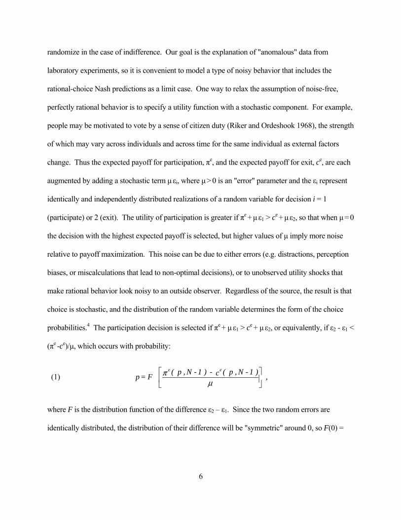
randomize in the case of indifference. Our goal is the explanation of "anomalous" data from

laboratory experiments, so it is convenient to model a type of noisy behavior that includes the

rational-choice Nash predictions as a limit case. One way to relax the assumption of noise-free,

perfectly rational behavior is to specify a utility function with a stochastic component. For example,

people may be motivated to vote by a sense of citizen duty (Riker and Ordeshook 1968), the strength

of which may vary across individuals and across time for the same individual as external factors

change. Thus the expected payoff for participation, πe, and the expected payoff for exit, ce, are each

augmented by adding a stochastic term µ εi, where µ > 0 is an "error" parameter and the εi represent

identically and independently distributed realizations of a random variable for decision i = 1

(participate) or 2 (exit). The utility of participation is greater if πe + µ ε1 > ce + µ ε2, so that when µ = 0

the decision with the highest expected payoff is selected, but higher values of µ imply more noise

relative to payoff maximization. This noise can be due to either errors (e.g. distractions, perception

biases, or miscalculations that lead to non-optimal decisions), or to unobserved utility shocks that

make rational behavior look noisy to an outside observer. Regardless of the source, the result is that

choice is stochastic, and the distribution of the random variable determines the form of the choice

probabilities.4 The participation decision is selected if πe + µ ε1 > ce + µ ε2, or equivalently, if ε2 - ε1 <

(πe -ce)/µ, which occurs with probability:

(1) e e( p , N - 1 ) - ( p , N - 1 )cp = F ,π

µ⎡ ⎤⎢ ⎥⎣ ⎦

where F is the distribution function of the difference ε2 – ε1. Since the two random errors are

identically distributed, the distribution of their difference will be "symmetric" around 0, so F(0) =

6

7

1/2.5 The error parameter, µ, determines the responsiveness of participation probabilities to

expected payoffs. Perfectly random behavior (i.e. p = 1/2) results as µ → ∞, since the argument of

the F(⋅) function on the right side of (1) goes to zero and F(0) = 1/2 as noted above. Perfect

rationality results in the limit as µ → 0, since the choice probability converges to 0 or 1, depending

on whether the expected participation payoff is less than or greater than the expected exit payoff.

More generally, for µ > 0, equation (1) expresses the participation probability as a noisy best

response to the expected payoff difference, which we will also refer to as a “stochastic best

response.”

Equation (1) characterizes a quantal response equilibrium (McKelvey and Palfrey 1995) if

the participation probability p in the expected payoff expressions on the right is equal to the choice

probability that emerges on the left.6 Without further parametric assumptions, there is no closed-

form solution for the equilibrium participation probability, but a simple graphical device can be used

to derive theoretical properties and characterize factors that might cause systematic deviations from

Nash predictions. The graph is based on a separation of the expected payoff difference from a term

that depends only on the noise elements (µ and the distribution of random elements). To this end,

apply the inverse of the F function to both sides of (1) and multiply by µ to obtain: µ F -1(p) =

πe(p, N-1) - ce(p, N-1). The determination of the equilibrium participation probability is illustrated in

Figure 1. As p goes from 0 to 1 on the horizontal axis, µ F -1(p) increases from -∞ to +∞, as shown

by the curved dark line with a positive slope in the figure.7 Since the expected payoff difference is

continuous in p, it has to cross the µ F -1(p) line at least once, which ensures existence of a symmetric

equilibrium.8 If the expected payoff difference πe(p, N-1) - ce(p, N-1) is decreasing in p, the

intersection will be unique. This case is illustrated in Figure 1, where the negatively sloped thin line

8

on the left side of the figure represents the expected payoff difference. This line intersects the

"inverse distribution" line at the equilibrium probability labeled QRE on the left. Also, notice that

the point where the expected payoff difference crosses the zero-payoff line constitutes a mixed-

strategy Nash equilibrium, since players are only willing to randomize if expected payoffs for the

two decisions are equal. This crossing point is labeled "NE Mix" in the figure.9

[Figure 1 goes about here]

Next consider the intuition for why the quantal response equilibrium is not typically at the

intersection of the expected-payoff-difference line and the zero-payoff horizontal line in the figure.

With equal expected payoffs for participation and exit, the person is indifferent and since F(0) = 1/2,

the stochastic best response to such indifference is to participate with probability 1/2. In the figure,

this result can be seen by starting where expected payoffs are equal at the NE Mix point on the left

and moving horizontally to the right, crossing the dark line at p = 1/2. This is not a quantal response

equilibrium since the p we started with (at the NE Mix) is not the stochastic best response to itself.

To find a stochastic best response to any given entry probability p on the horizontal axis, first move

in the vertical direction to find the associated expected payoff difference, and then move horizontally

(left or right) to the dark line, which determines the stochastic best response to that expected payoff

difference. Equilibrium requires that the stochastic best response to the others' participation

probability is that same probability, which occurs only at the intersection of the expected-payoff-

difference and inverse distribution lines in the figure. To summarize, a symmetric quantal response

probability is a stochastic best response to itself, whereas a symmetric Nash equilibrium probability

9

is a best response to itself.10

As long as the expected payoff difference is decreasing in p, it is apparent from Figure 1 that

any factor that increases the expected payoff difference line for all values of p will move the

intersection with the dark inverse distribution line to the right, and hence raise the quantal response

equilibrium probability. In an entry game, for example, the original π(n) function would be

decreasing if expected rewards are decreasing in the number of entrants, and it is then

straightforward to show that πe(N-1, p) is a decreasing function of both arguments.11 When the

opportunity cost payoff from not entering is constant, it follows that the expected payoff difference

πe(p, N-1) - ce(p, N-1) is decreasing in p and N, so a reduction in the number of potential entrants will

shift the thin line in the figure upward and raise the quantal response (QRE) probability, as

represented by a comparison of the high-N case on the left with the low-N case on the right.

The effect of additional "noise" in this model is easily represented, since an increase in the

error parameter µ makes the µF-1(p) line steeper around the midpoint, p = 1/2, although it still passes

through the zero-payoff line at this midpoint (see Figure 1). This increase in noise, therefore, moves

the quantal response equilibrium closer to 1/2, as would be expected. In contrast, as a reduction in µ

makes the µF-1(p) line flatter, and in the limit it converges to the horizontal line at zero as the noise

vanishes. In this case, the crossings for the QRE and mixed Nash equilibria match up, as would be

expected.

Next, consider coordination-type games where participation can be interpreted as an

individual decision of whether or not to help with a group production process that will only succeed

if enough people help out. For example, participation in revolutionary activities maybe individually

costly unless the movement reaches a critical mass. In such games, it does not pay to participate

10

unless enough others do, so π(n) will be less than c(n) for low n and greater than c(n) for high n.

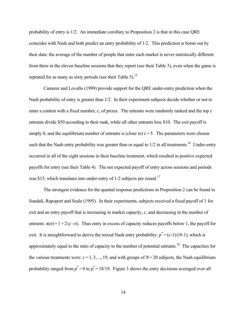
Thus the right side of (1) is increasing in the probability of participation. This property may result in

multiple quantal response equilibria since there can be multiple intersections when both the

expected-payoff-difference and the inverse distribution lines are increasing in p (see Figure 2, which

shows a case with three intersections). With multiple crossings, any factor that shifts the expected

payoff difference line upward will move some intersection points to the left and others to the right.

Thus the comparative statics effects are of opposite signs at adjacent equilibria, and we need to use

an analysis of dynamic adjustment to restrict consideration to equilibria that are stable (the

Samuelsonian "correspondence principle").12 A simple dynamic model can be based on the intuitive

idea that the participation probability will increase over time when the "noisy best response" to a

given p is higher than p. Thus dp/dt > 0 when F((πe(p, N-1) - ce(p, N-1))/µ) > p, or equivalently, p

would tend to increase when πe(p, N-1) - ce(p, N-1) > µ F -1(p) and decrease otherwise. For example,

start at p = .6 in Figure 2, which gives a positive expected payoff difference and a stochastic best

response of almost .9, found by moving horizontally to the right. For this reason, a rightward arrow

is present at p = .6 on the horizontal axis. The other directional arrows are found similarly, so there

is an unstable QRE at about .3, with arrows pointing away. In this manner it can be seen that the

quantal response equilibrium will be stable whenever the expected payoff difference line cuts the

inverse distribution line from above.

[Figure 2 goes about here]

Notice that any factor that raises the payoff from participation, and hence shifts the expected-

11

payoff-difference line upward in Figure 2, will raise the QRE participation probability if the

equilibrium is stable and not otherwise. To summarize:

Proposition 1. There is at least one symmetric quantal response equilibrium in a symmetric binary-

choice participation game. The equilibrium is unique if the difference between the expected payoff

of participating and exiting is decreasing in the probability of participation. In this case, any

exogenous factor that increases the participation payoff or lowers the exit payoff will raise the

equilibrium participation probability. The same comparative statics result holds when there are

multiple equilibria and attention is restricted to stable equilibria.

It is useful to begin with a discussion of entry games since they are the simplest application.

Moreover, the quantal response properties for these games also apply to the stable equilibria in more

complex applications such as threshold contribution games, volunteer's dilemma or voting. The

reader who is primarily in one of these subsequent applications may wish to skip any of the later

sections after reading as far as Proposition 2.

Entry Games: Under-Entry and Over-Entry Relative to Mixed-Nash Predictions

A widely studied example that fits the binary choice framework is an "entry" game, where

the choice is between a risky entry decision with high potential payoffs (if few others enter) and a

secure exit payoff. For example, entry may correspond to launching a political campaign, or filing

of an application for a limited number of public broadcast licenses. There are N potential entrants,

and we assume that if all others enter with probability 1, the representative player would prefer to

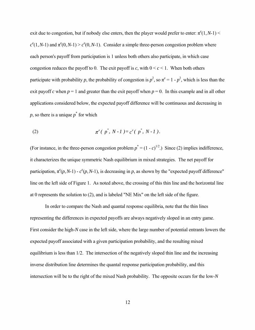
exit due to congestion, but if nobody else enters, then the player would prefer to enter: πe(1, N-1) <

ce(1, N-1) and πe(0, N-1) > ce(0, N-1). Consider a simple three-person congestion problem where

each person's payoff from participation is 1 unless both others also participate, in which case

congestion reduces the payoff to 0. The exit payoff is c, with 0 < c < 1. When both others

participate with probability p, the probability of congestion is p2, so πe = 1 - p2, which is less than the

exit payoff c when p = 1 and greater than the exit payoff when p = 0. In this example and in all other

applications considered below, the expected payoff difference will be continuous and decreasing in

p, so there is a unique p* for which

(2) * *e e ( , N - 1 ) = ( , N - 1 ) .p pcπ

(For instance, in the three-person congestion problem p* = (1 - c)1/2.) Since (2) implies indifference,

it characterizes the unique symmetric Nash equilibrium in mixed strategies. The net payoff for

participation, πe(p, N-1) - ce(p, N-1), is decreasing in p, as shown by the "expected payoff difference"

line on the left side of Figure 1. As noted above, the crossing of this thin line and the horizontal line

at 0 represents the solution to (2), and is labeled "NE Mix" on the left side of the figure.

In order to compare the Nash and quantal response equilibria, note that the thin lines

representing the differences in expected payoffs are always negatively sloped in an entry game.

First consider the high-N case in the left side, where the large number of potential entrants lowers the

expected payoff associated with a given participation probability, and the resulting mixed

equilibrium is less than 1/2. The intersection of the negatively sloped thin line and the increasing

inverse distribution line determines the quantal response participation probability, and this

intersection will be to the right of the mixed Nash probability. The opposite occurs for the low-N

12

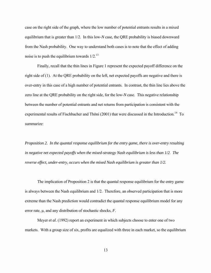
13

case on the right side of the graph, where the low number of potential entrants results in a mixed

equilibrium that is greater than 1/2. In this low-N case, the QRE probability is biased downward

from the Nash probability. One way to understand both cases is to note that the effect of adding

noise is to push the equilibrium towards 1/2.13

Finally, recall that the thin lines in Figure 1 represent the expected payoff difference on the

right side of (1). At the QRE probability on the left, net expected payoffs are negative and there is

over-entry in this case of a high number of potential entrants. In contrast, the thin line lies above the

zero line at the QRE probability on the right side, for the low-N case. This negative relationship

between the number of potential entrants and net returns from participation is consistent with the

experimental results of Fischbacher and Thöni (2001) that were discussed in the Introduction.14 To

summarize:

Proposition 2. In the quantal response equilibrium for the entry game, there is over-entry resulting

in negative net expected payoffs when the mixed-strategy Nash equilibrium is less than 1/2. The

reverse effect, under-entry, occurs when the mixed Nash equilibrium is greater than 1/2.

The implication of Proposition 2 is that the quantal response equilibrium for the entry game

is always between the Nash equilibrium and 1/2. Therefore, an observed participation that is more

extreme than the Nash prediction would contradict the quantal response equilibrium model for any

error rate, µ, and any distribution of stochastic shocks, F.

Meyer et al. (1992) report an experiment in which subjects choose to enter one of two

markets. With a group size of six, profits are equalized with three in each market, so the equilibrium

14

probability of entry is 1/2. An immediate corollary to Proposition 2 is that in this case QRE

coincides with Nash and both predict an entry probability of 1/2. This prediction is borne out by

their data: the average of the number of people that enter each market is never statistically different

from three in the eleven baseline sessions that they report (see their Table 3), even when the game is

repeated for as many as sixty periods (see their Table 5).15

Camerer and Lovallo (1999) provide support for the QRE under-entry prediction when the

Nash probability of entry is greater than 1/2. In their experiment subjects decide whether or not to

enter a contest with a fixed number, c, of prizes. The entrants were randomly ranked and the top c

entrants divide $50 according to their rank, while all other entrants lose $10. The exit payoff is

simply 0, and the equilibrium number of entrants is (close to) c + 5. The parameters were chosen

such that the Nash entry probability was greater than or equal to 1/2 in all treatments.16 Under-entry

occurred in all of the eight sessions in their baseline treatment, which resulted in positive expected

payoffs for entry (see their Table 4). The net expected payoff of entry across sessions and periods

was $15, which translates into under-entry of 1-2 subjects per round.17

The strongest evidence for the quantal response predictions in Proposition 2 can be found in

Sundali, Rapoport and Seale (1995). In their experiments, subjects received a fixed payoff of 1 for

exit and an entry payoff that is increasing in market capacity, c, and decreasing in the number of

entrants: π(n) = 1 + 2 (c - n). Thus entry in excess of capacity reduces payoffs below 1, the payoff for

exit. It is straightforward to derive the mixed Nash entry probability: p* = (c-1)/(N-1), which is

approximately equal to the ratio of capacity to the number of potential entrants.18 The capacities for

the various treatments were: c = 1, 3, ..., 19, and with groups of N = 20 subjects, the Nash equilibrium

probability ranged from p* = 0 to p* = 18/19. Figure 3 shows the entry decisions averaged over all

15

subjects, with the Nash predictions shown as the 45 degree line. Since each subject participated in

ten "runs" and there were three groups of twenty subjects, a data point in the figure is the average of

10*3*20 = 600 entry decisions. Note that the entry frequency is generally higher than predicted by

Nash for p* < 1/2 and lower than predicted for p* > 1/2, in line with the quantal response equilibrium

predictions.

[Figure 3 goes about here]

To summarize, the quantal response analysis explains the "magical" conformity to Nash

entry predictions (e.g. Meyer et al. 1992), the under-entry in the Camerer and Lovallo (1999)

baseline, the over-entry with many potential entrants observed by Fischbacher and Thöni (2001),

and the systematic pattern of deviations from Nash predictions reported by Sundali, Rapoport and

Seale (1995). This general approach can be adapted to evaluate behavior in other contexts where

payoffs for one decision are diminished as a result of congestion effects, as the next section

illustrates.19

The Volunteer's Dilemma

There are many situations in which a player's decision to participate benefits others. In

collective action problems, for instance, the contributions of some have positive returns for everyone

involved, and these returns are increasing in the number of contributors. In some contexts, the

critical number of participants is one, e.g. when a volunteer is needed to issue a politically risky veto

or sanction a group member who violated a norm. The dilemma in these situations is that

volunteering is costly and players have an incentive to free ride on others' benevolence.

[Table 1 goes here]

In the volunteer's dilemma game studied here (Diekmann 1986), all players receive a benefit

B if at least one of them incurs a cost, C < B. In this case, the expected payoff of participation, or

"volunteering" is simply a constant, B - C. The expected payoff from "exiting" follows from the

observation that when the N - 1 others volunteer with probability p, there is a (1 - p)N-1 chance that no

one volunteers, so ce(p, N-1) = B (1 - (1 - p)N-1). Notice that the volunteer's dilemma game satisfies

the assumptions underlying Figure 1, i.e. the difference between the expected payoffs of

participating and exiting is decreasing in p. The Nash probability of volunteering follows by

equating these expected payoffs (as per (2)) to obtain:

(3) 1

N - 1* C= 1 - .pB

⎛ ⎞⎜ ⎟⎝ ⎠

This probability of volunteering has the intuitive properties that it is increasing in the benefit, B,

decreasing in the cost, C, and decreasing in the number of potential volunteers, N. However, the

probability of getting no volunteers is (1-p*)N. By (3) the probability of getting no volunteers in a

Nash equilibrium is (C/B)N/(N-1), which is increasing in N, with lim N→∞ P(No Volunteer) = C/B > 0.

Unlike the intuitive comparative statics properties mentioned before, this prediction is not supported

by experimental data. Table 1 reports experimental results for a one-shot volunteer's dilemma game

with B = 100 and C = 50 (Franzen 1995). Notice that the probability that any person volunteers is

16

17

generally declining with N, as predicted by Nash.20 The probability that no one volunteers, however,

is decreasing in N and converges to 0 instead of C/B = 1/2.

Next, consider the quantal response equilibrium for the volunteer's dilemma. Since the

difference between the expected payoffs of volunteering and exiting is decreasing in the probability

of volunteering, Proposition 1 implies that the QRE probability of volunteering is unique, decreasing

in N and C, and increasing in B. Interestingly, the introduction of (enough) endogenous noise

reverses the unintuitive Nash prediction that the probability of "no volunteer" increases with N.

Proposition 3. In the quantal response equilibrium for the volunteer's dilemma game, the

probability that no one will volunteer is decreasing in the number of potential volunteers for a

sufficiently high error rate, µ. Furthermore, limN→∞ P(No Volunteer) = 0 for any µ > 0.

The proof of Proposition 3 is contained in the Appendix. The intuition is that, in the

presence of noise, the addition of potential volunteers only results in a small reduction in the

probability of volunteering, and the net effect is that the chance that someone volunteers will rise.21

The unintuitive feature of the Nash equilibrium for the volunteer's dilemma (i.e. that the

probability of getting no volunteer increases with N) parallels the result that the chance of convicting

an innocent defendant under the unanimity rule (i.e. no acquittal votes) rises with the size of the jury

(Feddersen and Pesendorfer 1998). The models differ in that jurors receive private signals about the

likelihood that the defendant is guilty. In the Nash equilibrium, those that receive a guilty signal

vote to convict while those with an innocent signal randomize between voting to convict or to

acquit. As the jury size increases, an individual juror's propensity to vote to acquit with an innocent

18

signal falls, and the chance that there is not a single vote to acquit rises. As a result, it becomes more

likely that an innocent defendant is wrongfully convicted (Feddersen and Pesendorfer 1998). In

laboratory jury voting experiments, subjects tend to vote strategically as predicted by the Nash

equilibrium. However, the unintuitive numbers effect is not supported by experimental data and is

not implied by a quantal response equilibrium analysis (Guarnaschelli, McKelvey, and Palfrey

2000).

Games with Multiple Equilibria: Step-Level Public Goods Games

In some binary-choice games the expected payoff function for participating is not decreasing

in p. For example, in any collective political activity where a critical mass is required to achieve a

desired outcome (e.g. regime change), the net reward from participating will be higher as others

become more involved.22 Therefore, the payoff difference function is increasing in the probability

of participation, which permits multiple crossings as shown in Figure 2. This is intuitive, since there

may exist both low-participation equilibria and high-participation equilibria in such "coordination"

or "assurance" games.23 A particular example is a step-level public goods game, where N players

decide whether or not to "contribute" at cost c. If the total number of contributions meets or exceeds

some threshold n*, then the public good is provided and all players receive a fixed return, V, whether

nor not they contributed. Here we assume that the contribution is like an effort that is lost if the

threshold is not met, so there is "no rebate." The threshold n* could correspond to a required number

of participants in an embargo or signatures on a petition.24

In the standard linear public goods games without a step, observed contributions in

experiments are positively related to the marginal effect of a contribution on the value of the public

good, known as the "marginal per capita return" (MPCR).25 Anderson, Goeree, and Holt (1998)

have shown that a logit quantal response analysis predicts this widely observed MPCR effect. This

raises the question whether there is a similar measure or index that would predict the level of

contributions in step-level public goods games. One would intuitively expect that contributions are

positively related to the total (social) value of the public good (NV) and negatively related to the

minimum total cost of providing it (n*c). Croson and Marks (2000) have proposed using the ratio of

social value to cost, which they call the "step return:" SR = NV/n*c. Based on a meta-analysis of

several step-level public goods games, they conclude "... subjects respond to the step return just as

they correspond to the marginal per capita return (MPCR) in linear public goods games: higher step

returns lead to more contributions."

First we consider whether there is a clear theoretical basis for expecting contributions to be

positively related to step return measures. A contribution in this game pays off only when it is

pivotal, i.e. when exactly n* - 1 others contribute, which happens with probability

(4) * * - 1 N - n n

*

N - 1 ( 1 - p ,p )

- 1 n⎛ ⎞⎜ ⎟⎝ ⎠

where, as before, p denotes the probability that others participate. The difference between the

expected payoff of contributing or not contributing is therefore:

(5) * * - 1 N - n ne e

*

N - 1 ( p, N - 1 ) - ( p, N - 1 ) = V ( 1 - p - c .p )c

- 1 nπ

⎛ ⎞⎜ ⎟⎝ ⎠

The right side is a single-peaked function of p, and equating its derivative to 0 yields a unique

maximum at p = (n* - 1)/(N - 1). Figure 4, drawn for V = 6, c = 1, and N = 10, shows these "hill

19

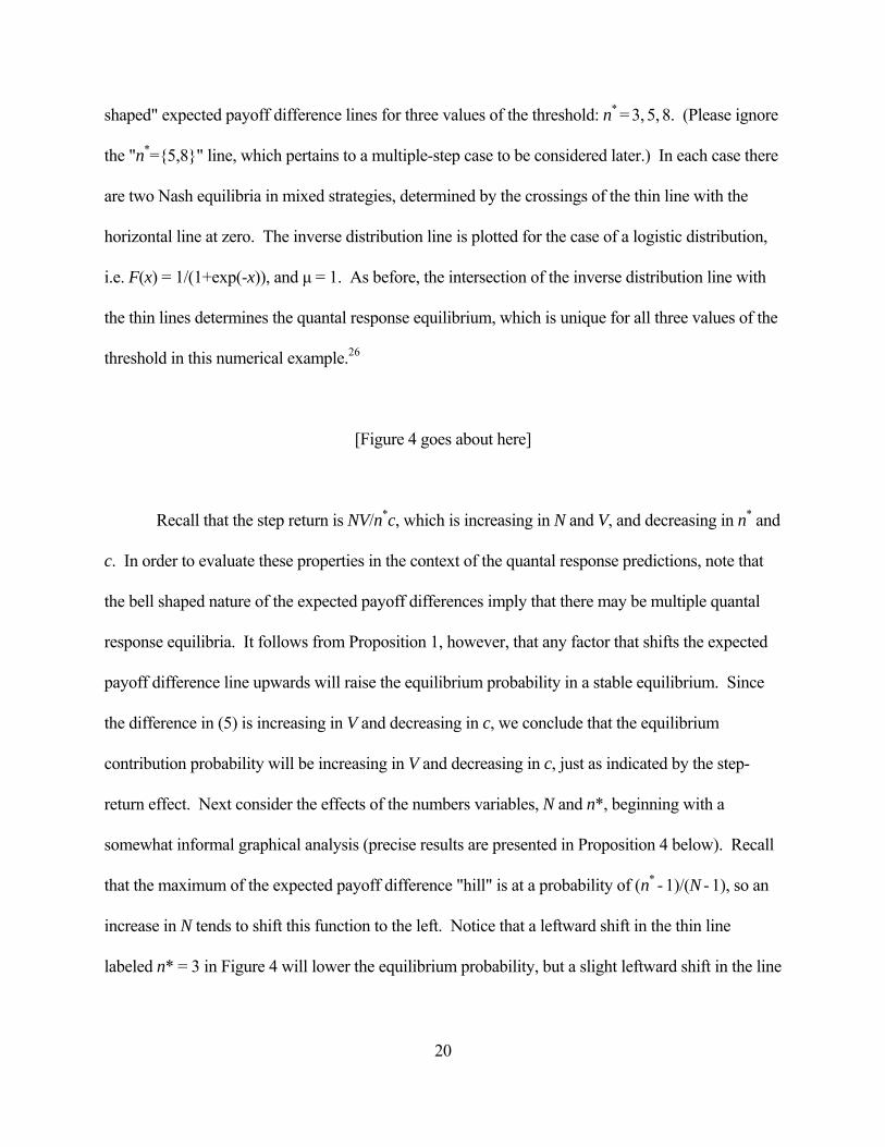
20

shaped" expected payoff difference lines for three values of the threshold: n* = 3, 5, 8. (Please ignore

the "n*={5,8}" line, which pertains to a multiple-step case to be considered later.) In each case there

are two Nash equilibria in mixed strategies, determined by the crossings of the thin line with the

horizontal line at zero. The inverse distribution line is plotted for the case of a logistic distribution,

i.e. F(x) = 1/(1+exp(-x)), and µ = 1. As before, the intersection of the inverse distribution line with

the thin lines determines the quantal response equilibrium, which is unique for all three values of the

threshold in this numerical example.26

[Figure 4 goes about here]

Recall that the step return is NV/n*c, which is increasing in N and V, and decreasing in n* and

c. In order to evaluate these properties in the context of the quantal response predictions, note that

the bell shaped nature of the expected payoff differences imply that there may be multiple quantal

response equilibria. It follows from Proposition 1, however, that any factor that shifts the expected

payoff difference line upwards will raise the equilibrium probability in a stable equilibrium. Since

the difference in (5) is increasing in V and decreasing in c, we conclude that the equilibrium

contribution probability will be increasing in V and decreasing in c, just as indicated by the step-

return effect. Next consider the effects of the numbers variables, N and n*, beginning with a

somewhat informal graphical analysis (precise results are presented in Proposition 4 below). Recall

that the maximum of the expected payoff difference "hill" is at a probability of (n* - 1)/(N - 1), so an

increase in N tends to shift this function to the left. Notice that a leftward shift in the thin line

labeled n* = 3 in Figure 4 will lower the equilibrium probability, but a slight leftward shift in the line

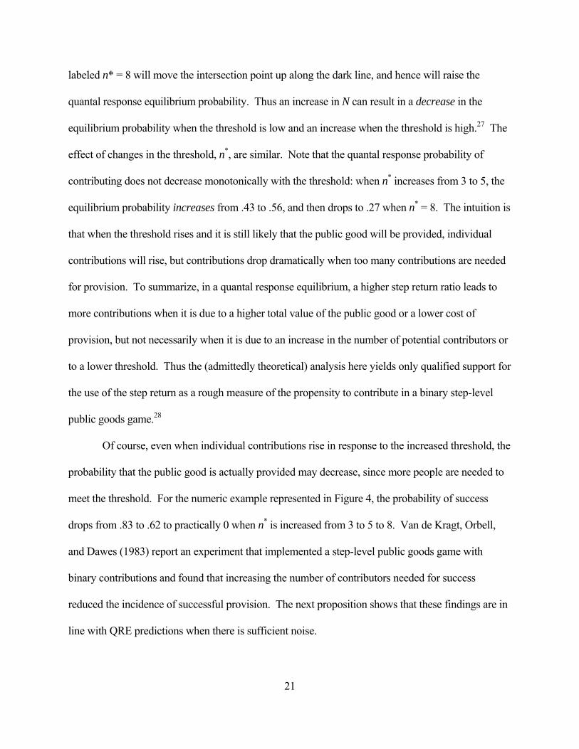
21

labeled n* = 8 will move the intersection point up along the dark line, and hence will raise the

quantal response equilibrium probability. Thus an increase in N can result in a decrease in the

equilibrium probability when the threshold is low and an increase when the threshold is high.27 The

effect of changes in the threshold, n*, are similar. Note that the quantal response probability of

contributing does not decrease monotonically with the threshold: when n* increases from 3 to 5, the

equilibrium probability increases from .43 to .56, and then drops to .27 when n* = 8. The intuition is

that when the threshold rises and it is still likely that the public good will be provided, individual

contributions will rise, but contributions drop dramatically when too many contributions are needed

for provision. To summarize, in a quantal response equilibrium, a higher step return ratio leads to

more contributions when it is due to a higher total value of the public good or a lower cost of

provision, but not necessarily when it is due to an increase in the number of potential contributors or

to a lower threshold. Thus the (admittedly theoretical) analysis here yields only qualified support for

the use of the step return as a rough measure of the propensity to contribute in a binary step-level

public goods game.28

Of course, even when individual contributions rise in response to the increased threshold, the

probability that the public good is actually provided may decrease, since more people are needed to

meet the threshold. For the numeric example represented in Figure 4, the probability of success

drops from .83 to .62 to practically 0 when n* is increased from 3 to 5 to 8. Van de Kragt, Orbell,

and Dawes (1983) report an experiment that implemented a step-level public goods game with

binary contributions and found that increasing the number of contributors needed for success

reduced the incidence of successful provision. The next proposition shows that these findings are in

line with QRE predictions when there is sufficient noise.

22

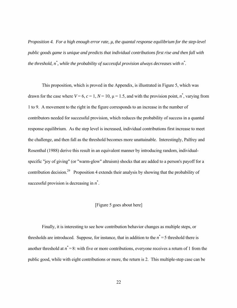
Proposition 4. For a high enough error rate, µ, the quantal response equilibrium for the step-level

public goods game is unique and predicts that individual contributions first rise and then fall with

the threshold, n*, while the probability of successful provision always decreases with n*.

This proposition, which is proved in the Appendix, is illustrated in Figure 5, which was

drawn for the case where V = 6, c = 1, N = 10, µ = 1.5, and with the provision point, n*, varying from

1 to 9. A movement to the right in the figure corresponds to an increase in the number of

contributors needed for successful provision, which reduces the probability of success in a quantal

response equilibrium. As the step level is increased, individual contributions first increase to meet

the challenge, and then fall as the threshold becomes more unattainable. Interestingly, Palfrey and

Rosenthal (1988) derive this result in an equivalent manner by introducing random, individual-

specific "joy of giving" (or "warm-glow" altruism) shocks that are added to a person's payoff for a

contribution decision.29 Proposition 4 extends their analysis by showing that the probability of

successful provision is decreasing in n*.

[Figure 5 goes about here]

Finally, it is interesting to see how contribution behavior changes as multiple steps, or

thresholds are introduced. Suppose, for instance, that in addition to the n* = 5 threshold there is

another threshold at n* = 8: with five or more contributions, everyone receives a return of 1 from the

public good, while with eight contributions or more, the return is 2. This multiple-step case can be

23

analyzed in the same manner as before. Now there are two points at which one's contribution can be

pivotal, and the expected payoff is the sum of the two effects. In terms of Figure 4, the expected

payoff lines for n* = 5 and n* = 8 get "summed," as indicated by the n* = {5,8} line in Figure 4 (the

cost of contributing only enters once, which is why the endpoints of the dotted line are still at -1).

The introduction of the extra threshold at n* = 8, which by itself results in a low contribution

probability, dramatically increases contributions: the QRE contribution probability is .73 and the

probability that at least five people contribute is as high as .97. An immediate extension of this

analysis is that adding more steps, without reducing the payoff increment at any of the existing steps,

will increase quantal response contribution probabilities in a binary public goods game.

Voting Participation Games

Another binary choice of considerable interest is the decision of whether or not to vote in a

small-group situation where voting is costly and a single vote has a non-negligible effect on the final

outcome, e.g. the decision of whether to attend a faculty meeting on a busy day. The analysis is

similar to that of a step-level public goods game, since the threshold contribution, n*, corresponds to

the number of votes needed to pass a favored bill. In a real voting contest, however, the vote total

required to win is endogenously determined by the number of people voting against the bill. If there

are two types of voters, those who favor a bill and those who oppose, then the equilibrium will be

characterized by a participation probability for each type. Here we restrict attention to a symmetric

model with equal numbers of voters of each type, equal costs of voting, c, and symmetric valuations:

V if the preferred outcome receives more votes and 0 otherwise. Ties in this majority rule game are

decided by the flip of a coin. Note that the public goods incentives to free ride are still present in this

game, since voters benefit when their side wins, regardless of whether or not they incurred the cost

of voting.

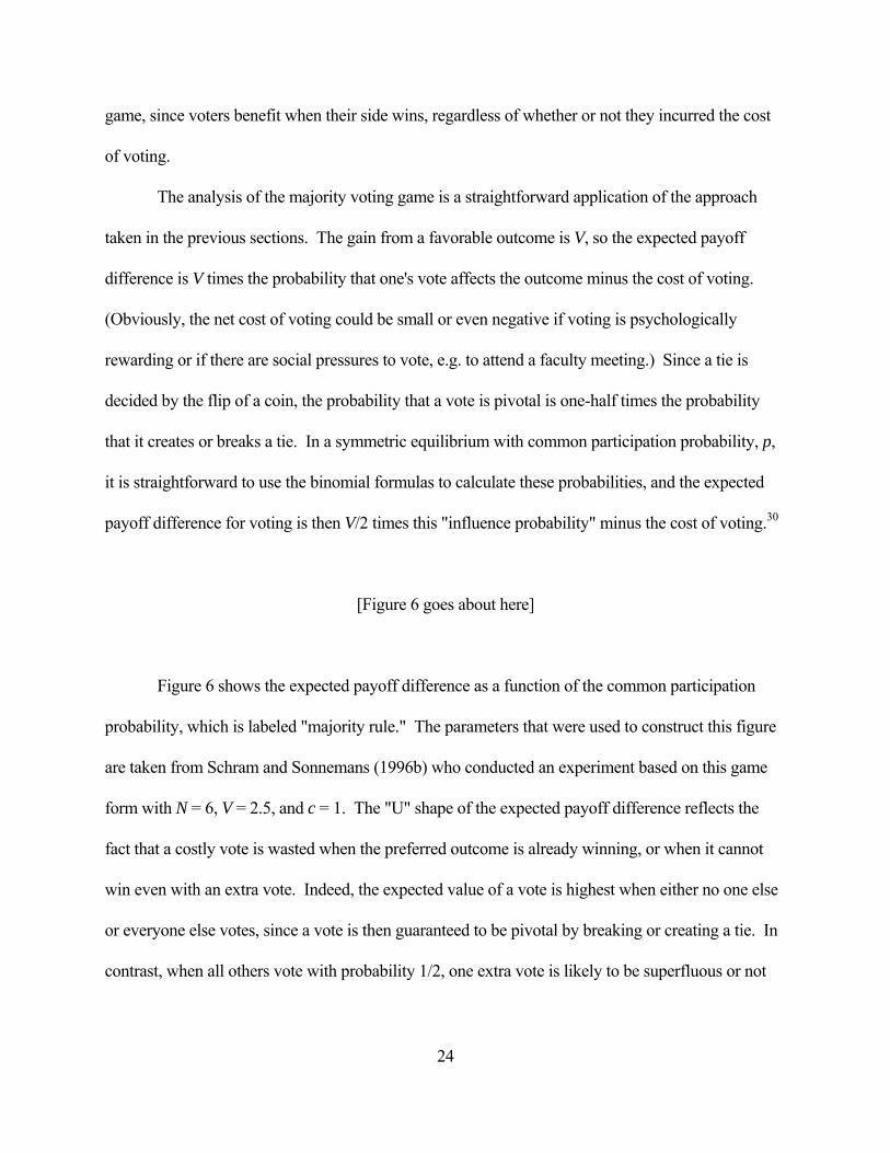
The analysis of the majority voting game is a straightforward application of the approach

taken in the previous sections. The gain from a favorable outcome is V, so the expected payoff

difference is V times the probability that one's vote affects the outcome minus the cost of voting.

(Obviously, the net cost of voting could be small or even negative if voting is psychologically

rewarding or if there are social pressures to vote, e.g. to attend a faculty meeting.) Since a tie is

decided by the flip of a coin, the probability that a vote is pivotal is one-half times the probability

that it creates or breaks a tie. In a symmetric equilibrium with common participation probability, p,

it is straightforward to use the binomial formulas to calculate these probabilities, and the expected

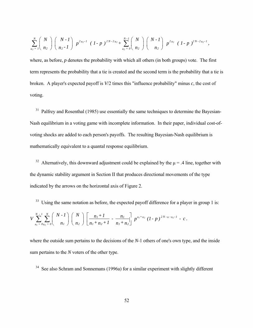
payoff difference for voting is then V/2 times this "influence probability" minus the cost of voting.30

[Figure 6 goes about here]

Figure 6 shows the expected payoff difference as a function of the common participation

probability, which is labeled "majority rule." The parameters that were used to construct this figure

are taken from Schram and Sonnemans (1996b) who conducted an experiment based on this game

form with N = 6, V = 2.5, and c = 1. The "U" shape of the expected payoff difference reflects the

fact that a costly vote is wasted when the preferred outcome is already winning, or when it cannot

win even with an extra vote. Indeed, the expected value of a vote is highest when either no one else

or everyone else votes, since a vote is then guaranteed to be pivotal by breaking or creating a tie. In

contrast, when all others vote with probability 1/2, one extra vote is likely to be superfluous or not

24

enough and its expected value is therefore small. As in previous sections, the mixed Nash prediction

is determined by where the expected payoff difference line crosses the zero line: there are two Nash

equilibria, one in which almost no one votes and another in which almost everyone votes (Palfrey

and Rosenthal 1983).

The quantal response equilibrium is determined by the intersection of the expected payoff

difference line and the inverse distribution function (dark lines).31 The µ parameter of 0.8 used to

construct the steeper line was selected so that the QRE prediction would be at about the same level

(30 to 50 percent) as the vote participation probabilities reported by Schram and Sonnemans (1996b)

in the initial periods of their experiment. Interestingly, the voting probabilities started high and then

decreased to stabilize somewhere in the 20 to 30 percent range. This downward trend is crudely

captured by a reduction in the noise parameter µ to 0.4 as indicated by the second inverse

distribution line in Figure 6.32

Schram and Sonnemans (1996b) also considered a "proportional rule" game in which each

person's payoff is the proportion of votes for their preferred outcome, minus the cost of voting if they

voted. Again, it is straightforward to use the binomial formula to calculate the expected proportion

of favorable votes, contingent on one's own decision of whether to vote, as a function of the common

participation probability, p.33 The expected payoff difference for this proportional representation

game is the increase in the expected proportion of favorable votes, minus the cost of voting. This

difference is declining everywhere because one's vote has a smaller impact on the vote proportion as

the probability of others' participation increases. The expected payoff difference line is labeled

"proportional rule" in Figure 6, where the parameters are again taken from Schram and Sonnemans

(1996b): N = 6, V = 2.22, and c = 0.7. The Schram and Sonnemans data for the proportional rule

25

26

experiments, plotted as the lower line in Figure 7, started in the 30 to 40 percent range and ended up

between 20 and 30 percent in the final periods. Note that participation is initially higher with the

majority rule than with the proportional rule, while this difference disappears in the final periods of

the experiment when the voting probabilities are close to 25 percent, well above the Nash

predictions for these games. This result is not surprising from a QRE point of view, since the two

expected payoff difference lines cross at p = .25 at which they intersect with the inverse distribution

line (for µ = 0.4). The result, however, is unexplainable by a Nash analysis for which the

intersection of the two expected payoff difference lines plays no role and only "crossings at zero"

matter. For the parameter values of the experiment, these crossings are at p = .05 and p = .95 for the

majority rule treatment and at p = .09 for the proportional rule treatment, and seem to have little

predictive power for the results of the Schram and Sonnemans (1996b) experiment.34 To

summarize, both the qualitative data patterns as well as the magnitude of the observed voting

probabilities are consistent with a QRE analysis (but not with Nash), as can be seen from Figures 6

and 7.35

[Figure 7 goes about here]

This general approach may be extended to cover cases with asymmetries, e.g. when one type

is more numerous than another. With asymmetries, the equilibrium will consist of a participation

probability for each type. These two probabilities will be determined by two equations analogous to

(1), with the expected payoff for participation (voting) being a function of the number of potential

voters of each type and the equilibrium participation probabilities. While a simple graphical analysis

27

of this asymmetric model is not possible, it is straightforward to proceed with numerical

calculations, for example, to show that the smaller group is more likely to vote when the costs of

voting are symmetric (Palfrey and Rosenthal 1983).36

Conclusion

Many strategic situations are characterized by binary decisions, e.g. whether or not to vote,

volunteer, attend a congested event, or perform a costly task with social benefits. In this paper we

present a simple model of equilibrium behavior that applies to a wide variety of seemingly unrelated

binary-choice games, including coordination, public goods, entry, voting participation, and

volunteer's dilemma games. The model captures the feature that the decision of whether or not to

participate may be affected by randomness, either in preferences (e.g. entry or voting costs) or in

decision making (due to perception or calculation errors). The resulting quantal response

equilibrium (McKelvey and Palfrey 1995) incorporates this randomness in the form of an error

parameter and nests the standard rational-choice Nash equilibrium as a limiting case.

The quantal response equilibrium tracks many behavioral deviations from Nash predictions,

e.g. the tendency for entry to match the Nash predictions when the prediction is 1/2, and for excess

entry when the Nash prediction is below 1/2. In other words, a model with behavioral noise is

capable of explaining the "magical" accuracy of Nash predictions in some experiments and the

systematic deviations in others. The observed over-entry when Nash predictions are low is

analogous to the over-participation in voting experiments, which is explained by a quantal response

analysis. The participation rates in these experiments are roughly the same for the majority and

proportional outcome rule treatments, which are consistent with theoretical calculations for the

28

parameters used in the experiments. Similarly, the quantal response model tracks intuitive "numbers

effects" observed in volunteers' dilemma and step-level public goods experiments, both when these

effects are consistent with Nash predictions and when they are not.

The quantal response equilibrium generalizes the standard Nash theory by allowing for

stochastic elements. The scale of these elements, as measured by the error rate µ, determines how

closely decisions match perfect-rationality predictions. Despite the unspecified nature of the

stochastic elements, the quantal response equilibrium provides clear, falsifiable predictions for many

of the binary-choice models considered in this paper. For example, the predicted participation

probabilities for the entry games are less extreme than Nash predictions (i.e. they lie between 1/2

and the mixed-strategy Nash equilibrium) for any error distribution F. Similarly, the predicted

volunteer rates for the volunteer's dilemma are less extreme than Nash since the expected payoff

difference is decreasing in the probability of volunteering. In addition, there are key differences

between Nash and quantal response equilibrium predictions such as the effect of large numbers on

the probability of getting at least one volunteer or one vote to acquit under unanimity.

Taken together, these results indicate that standard "rational-choice" game theory can be enriched in

a manner that increases its behavioral relevance for a wide class of situations. Moreover, the simple

nature of the graphical equilibrium analysis will aid researchers in other binary choice applications.

Appendix

Proof of Proposition 3. The probability, P, that no one volunteers is given by (1-p)N, where the

QRE probability of volunteering, p, satisfies:

(A1) N - 1-1 ( p ) = B ( 1 - p - C .)Fµ

Combining these equations and using the fact that F-1(p) is symmetric, i.e. F-1(p) = - F-1(1-p), allows

one to express (A1) in terms of the probability that no one volunteers:

(A2) N - 11N N F( ) = C - B P Pµ

from which the derivative of P with respect to N can be established as:

Log -1 1/ N -1 + 2/N

-1 1/ N -1 + 2/N

d P P ( P ) B f ( ( )) - F P P = - d N N (N - 1) B f ( ( )) + F P P

µµ

Note that dP/dN can only be non-negative when µ ≤ P1-2/N B f(F-1(P1/N)). The right side of this

inequality is bounded by B max(f), so dP/dN has to be negative for large enough µ. Finally, suppose,

in contradiction, that limN→∞ P > 0. This implies that P1/N tends to 1, so µ F-1(P1/N) → ∞ when µ > 0.

This contradicts (A2) since the right side limits to C - B P, which is finite. Hence, P tends to zero

when N tends to infinity. In fact, from (A2) it follows that for large N, P converges to F(C/µ)N,

which tends to zero since F(C/µ) < 1 for µ > 0. Q.E.D.

29

Proof of Proposition 4. The QRE probability of contributing, p, satisfies:

(A3) N-1w ( p ) = V ( p ) - c ,F Pµ

where w ≥ 1 denotes the threshold and PwN(p) is the probability that w-1 out of the N-1 others

contributed (see equation (6)). The solution to (A3) is unique when the derivative of the left side is

everywhere greater than that of the right side. The derivative of PwN(p) with respect to p is given by

((w-1)/p - (N-w)/(1-p)) PwN(p) and the relevant condition for uniqueness is therefore:

(A4) N-1w > V f ( ( p )) ((w - 1)/p - (N - w)/(1 - p)) ,F Pµ

Note that the right side is negative when w = 1 and for w ≥ 2 it is less than V f(F-1(p))PwN (w-1)/p. The

latter expression can be rewritten as (N-1) V f(F-1(p))Pw-1N-1, which is bounded by (N-1) V max(f). So

for µ > (N-1) V max(f), the quantal response probability of contributing is unique for all values of the

threshold. The derivative of PwN(p) with respect to w < N (holding p fixed) is Pw+1

N(p) - PwN(p),

which simplifies to: PwN(p) (1 - w/(N-w) (1-p)/p). Together with (A3) this implies that the derivative

of the QRE probability, p, with respect to the threshold, w, is given by:

(A5) N-1

wN-1

w

d p 1 - p V f ( ( p )) ((N - w)/(1 - p) - w/p ) F P = ,d w N - w + V f ( ( p )) ((N - w)/(1 - p) - (w - 1)/p) F Pµ

Note that the denominator of the second fraction on the right side is positive when the condition for a

unique QRE (eq. (A4)) is satisfied. The sign of dp/dw is then determined by the numerator which is

positive iff p ≥ w/N. The intuition for this result is straightforward: as long as the "inverse

distribution" line intersects the "expected payoff difference" line to the right of its maximum (i.e. p >

w/N), an increase in w shifts the expected payoff difference to the right and moves the intersection

30

point upwards. The reverse happens for higher values of w when the inverse distribution line cuts

the expected payoff difference line to the left of the maximum (see also Palfrey and Rosenthal

1982).

The probability, QwN, that the public good is provided is given by

31

- k N

N k N w

k = w

N = ( 1 - p ,Q p )

k ⎛ ⎞⎜ ⎟⎝ ⎠

∑

and its derivative with respect to w (for w < N) is:

(A6) N N

N N Nw www + 1 w

d d Q Q d p d p 1 - p = - + = N - .Q Q Pd w d p d w d w N - w⎛ ⎞⎜ ⎟⎝ ⎠

Combining (A5) and (A6) shows that QwN is decreasing in w. Q.E.D.

32

References

Anderson, Simon P., Jacob K. Goeree, and Charles A. Holt. 1998. "A Theoretical Analysis of

Altruism and Decision Error in Public Goods Games." Journal of Public Economics 70: 297-

323.

Anderson, Simon P., Jacob K. Goeree, and Charles A. Holt. 2002. "The Logit Equilibrium: A

Perspective on Intuitive Behavioral Anomalies." Southern Economic Journal 69 (1): 21-47.

Camerer, Colin, and D. Lovallo. 1999. “Overconfidence and Excess Entry: An Experimental

Approach.” American Economic Review 89 (March): 306-318.

Capra, C. Monica, Jacob K. Goeree, Rosario Gomez, and Charles A. Holt. 1999. "Anomalous

Behavior in a Traveler's Dilemma?" American Economic Review 89 (June): 678-690.

Cohen, Linda R. and Roger Noll. 1991. "How to Vote, Whether to Vote: Strategies for Voting and

Abstaining on Congressional Roll Calls." Political Behavior 13(2): 97-127.

Chong, Dennis. 1991. Collective Action and the Civil Rights Movement. Chicago: University of

Chicago Press.

Croson, Rachel T.A., and Melanie Beth Marks. 2000. "Step Returns in Threshold Public Goods: A

Meta- and Experimental Analysis." Experimental Economics 2 (3): 239-259.

Diekmann, Andreas. 1985. "Volunteer's Dilemma." Journal of Conflict Resolution. 29 (4): 605-610.

Diekmann, Andreas. 1986. "Volunteer's Dilemma: A Social Trap Without a Dominant Strategy and

Some Empirical Results." In Paradoxical Effects of Social Behavior: Essays in Honor of

Anatol Rapoport, eds. A. Diekmann and P. Mitter. Heidelberg: Physica-Verlag, 187-197.

Erev, Ido, and Amnon Rapoport. 1998. “Coordination, "Magic," and Reinforcement Learning in a

33

Market Entry Game.” Games and Economic Behavior 23 (May): 146-175.

Erev, Ido, Amnon Rapoport, Darryl A. Seale, and James A. Sundali. 1998. “Equilibrium Play in

Large Market Entry Games.” Management Science 44: 119-141.

Feddersen, Timothy and Wolfgang Pesendorfer. 1998. "Convicting the Innocent: The Inferiority of

Unanimous Jury Verdicts under Strategic Voting." American Political Science Review 92:

23-36.

Fey, Mark. 1997. "Stability and Coordination in Duverger's Law: A Formal Model of Preelection

Polls and Strategic Voting." American Political Science Review 91 (1): 135-147.

Fischbacher, Urs, and Christian Thöni. 2001. “Inefficient Excess Entry in an Experimental Winner-

Take-All Market.” University of Zurich, Working paper No. 86.

Franzen, A. 1995. "Group Size and One Shot Collective Action." Rationality and Society 7: 183-

200.

Gilligan, Michael J. 2003. "Is there a Broader-Deeper Tradeoff?" New York University, Photocopy.

Goeree, Jacob K. and Charles A. Holt. 1999. "Stochastic Game Theory: For Playing Games, Not

Just for Doing Theory." Proceedings of the National Academy of Sciences 96 (September):

10564-10567.

Guarnaschelli, Serena, Richard D. McKelvey and Thomas R. Palfrey. 2000. "An Experimental

Study of Jury Decision Making." American Political Science Review 94 (2): 407-423.

Kahneman, Daniel. 1988. "Experimental Economics: A Psychological Perspective." In Bounded

Rational Behavior in Experimental Games and Markets. Eds. R. Tietz, W. Albers, and R.

Selten. New York: Springer-Verlag, 11-18.

Lohmann, Susanne. 1994. “Dynamics of Informational Cascades: The Monday Demonstrations in

34

Leipzig, East Germany, 1989-1991.” World Politics 47: 42-101.

McKelvey, Richard D. and Thomas R. Palfrey. 1995. "Quantal Response Equilibria for Normal

Form Games." Games and Economic Behavior 10: 6-38.

Meyer, Donald J., John B. Van Huyck, Raymond C. Battalio, and Thomas R. Saving. 1992.

“History's Role in Coordinating Decentralized Allocation Decisions: Laboratory Evidence

on Repeated Binary Allocation Games.” Journal of Political Economy 100 (April): 292-316.

Miller, Gary J. 1997. "The Impact of Economics on Contemporary Political Science." Journal of

Economic Literature 35: 1173-1204.

Morgan, Dylan, Anne M. Bell, and William A. Sethares. 1999. "An Experimental Study of the El

Farol Problem." Discussion Paper, presented at the Summer ESA Meetings, Tucson.

Morton, Rebecca. 1999. Methods and Models: A Guide to the Empirical Analysis of Formal Models

in Political Science. Cambridge: Cambridge University Press.

Ochs, Jack. 1990. “The Coordination Problem in Decentralized Markets: An Experiment.”

Quarterly Journal of Economics 105 (May): 545-559.

Offerman, Theo, Arthur Schram and Joep Sonnemans. 1998. "Quantal Response Models in Step-

Level Public Goods." European Journal of Political Economy. 14: 89-100.

Ordeshook, Peter C. 1986. Game Theory and Political Theory. Cambridge: Cambridge University

Press.

Ostrom, Elinor. 1998. "A Behavioral Approach to the Rational Choice Theory of Collective Action."

American Political Science Review 92 (1): 1-22.

Palfrey, Thomas R. and Howard Rosenthal. 1983. "A Strategic Calculus of Voting." Public Choice

41: 7-53.

35

Palfrey, Thomas R. and Howard Rosenthal. 1985. "Voter Participation and Strategic Uncertainty."

American Political Science Review 79: 62-78.

Palfrey, Thomas R. and Howard Rosenthal. 1988. "Private Incentives in Social Dilemmas." Journal

of Public Economics 35: 309-332.

Rapoport, Amnon. 1995. “Individual Strategies in a Market Entry Game.” Group Decision and

Negotiation 4: 117-133.

Rapoport, Amnon, Darryl A. Seale, and Lisa Ordonez. 2002. "Weighted Probabilities in Large

Group Coordination: Theory and Experimental Evidence from Market Entry Games."

Journal of Risk and Uncertainty 25: 21-45.

Rapoport, Amnon, Darryl A. Seale, Ido Erev, and James A. Sundali. 1998. "Equilibrium Play in

Large Group Market Entry Games." Management Science 44 (January): 119-141.

Rapoport, Amnon, and James A. Sundali. 1997. “Induction vs. Deterrence in the Chain Store Game:

How Many Potential Entrants Are Needed to Deter Entry?” In Understanding Strategic

Behavior: Essays in Honor of Reinhard Selten. Eds. W. Albers, Werner Guth, P.

Hammerstein, B. Moldovanu and E. van Damme. Berlin: Springer-Verlag.

Riker, William H. and Peter Ordeshook. 1968. "Theory of the Calculus of Voting." American

Political Science Review 62 (1): 25-43.

Schram, Arthur, and Joep Sonnemans. 1996a. “Voter Turnout as a Participation Game: An

Experimental Investigation.” International Journal of Game Theory 25 (3): 385-406.

Schram, Arthur, and Joep Sonnemans. 1996b. “Why People Vote: Experimental Evidence.” Journal

of Economic Psychology 17: 417-442.

Signorino, Curtis S. 1999. "Strategic Interaction and the Statistical Analysis of International

36

Conflict." American Political Science Review 93 (June): 279-297.

Sundali, James A., Amnon Rapoport, and Darryl A. Seale. 1995. “Coordination in Market Entry

Games with Symmetric Players.” Organizational Behavior and Human Decision Processes

64: 203-218.

van de Kragt, Alphons, John M. Orbell, and Robyn M. Dawes. 1983. “The Minimal Contributing

Set as a Solution to Public Goods Problems.” American Political Science Review 77

(March): 112-122.

TABLE 1. Frequencies of Individual Volunteer Decisions (p) and of "No Volunteer" Outcomes,

N p P(No Volunteer)

2 .65 .12

3 .58 .07

5 .43 .06

7 .25 .13

9 .35 .02

21 .30 .00

51 .20 .00

101 .35 .00

Source: Franzen (1995).

37

FIGURE 1. Quantal Response and Nash Participation Probabilities for Low-N and High-N Cases

38

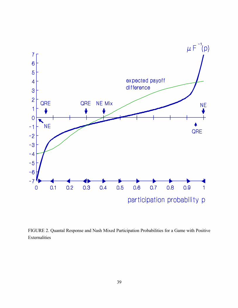
FIGURE 2. Quantal Response and Nash Mixed Participation Probabilities for a Game with Positive Externalities

39

FIGURE 3. Nash Predictions (solid line) and Observed Entry Probabilities (diamonds) Source: Sundali, Rapoport, and Seale (1995)

40

FIGURE 4. Expected Payoff Differences and the Inverse Distribution Line for Different Thresholds in Step-Level Public Goods Games

41

FIGURE 5. QRE Probabilities of Individual Contribution and Successful Group Provision of a Step Level Public Good, as a Function of the Provision Point

42

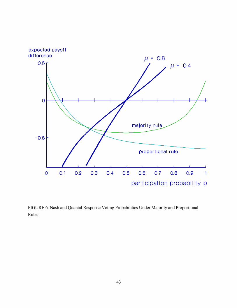
FIGURE 6. Nash and Quantal Response Voting Probabilities Under Majority and Proportional Rules

43

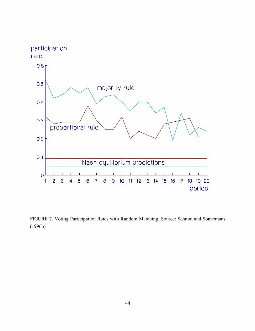
FIGURE 7. Voting Participation Rates with Random Matching, Source: Schram and Sonnemans (1996b)

44

45

Endnotes

* Goeree: Division of the Humanities and Social Sciences, California Institute of Technology,

Mail code 228-77, Pasadena, CA 91125, USA. Holt: Department of Economics, University of

Virginia, Charlottesville, VA 22904-4182. We gratefully acknowledge financial support from the

National Science Foundation (SBR-0094800), the Alfred P. Sloan Foundation, the Bankard Fund at

the University of Virginia, and the Dutch National Science Foundation (VICI 453.03.606). This

paper benefitted from comments provided by three anonymous referees, Rebecca Morton, Howard

Rosenthal, and participants at the quantal response workshop at Caltech and the Politics seminar at

NYU.

1 Entry decisions in this context are known as the "El Farol" dilemma, named after a popular

bar in Santa Fe (Morgan, Dylan, Bell, and Sethares 1999).

2 This successful coordination has been explained by models of adaptation and learning (Meyer,

Van Huyck, Battalio, and Saving 1992; Erev and Rapoport 1998).

3 The participation game terminology was introduced by Palfrey and Rosenthal (1983) in the

context of the decision of whether or not to vote. These voting participation games are discussed in

section 6 below.

4 For instance, a normal distribution yields the probit model, while a double exponential

distribution gives rise to the logit model, in which case the choice probabilities are proportional

exponential functions of expected payoffs.

46

5 More formally, Pr(ε1 ≤ ε2) = 1/2, so Pr(ε1 - ε2 ≤ 0) = F(0) = 1/2.

6 The quantal response equilibrium, developed by political scientists (McKelvey and Palfrey

1995), has been applied to the study of international conflict by Signorino (1999). A general

introduction to the usefulness of the quantal response approach in the analysis of political data can

be found in Morton (1999).

7 To see this, note that an expected payoff difference of -∞ on the vertical axis will cause the

participation probability to be 0, and an expected payoff difference of +∞ will cause the

participation probability to be 1. This is why the dark "inverse distribution" line starts at -∞ on the

left side of Figure 1 and goes to +∞ on the right.

8 The existence of quantal response equilibria for normal-form games with a finite number of

strategies is proved in McKelvey and Palfrey (1995) and for normal-form games with a continuous

strategy space in Anderson, Goeree, and Holt (2002).

9 All the games considered in this paper are symmetric in the sense that players’ payoff

functions are identical. We will only consider symmetric mixed-strategy Nash equilibria for

such games. It is sometimes possible to find asymmetric Nash equilibria for symmetric games

but without some coordination device these equilibria seem less plausible.

10 At the "NE Mix" point in Figure 1, expected payoffs are equal and any probability is a best

response, so the NE Mix probability is a best response to itself.

47

11 Intuitively, holding N fixed, a higher probability of entering means that more people enter,

which results in a lower expected payoff of entry. Similarly, holding p fixed, a higher number of

potential entrants results in more entry. This can be made more precise as follows: suppose N is

fixed and the entry probability is p1. Let the number of entrants be determined by drawing a

random number that is uniformly distributed on [0, 1] for each player. If the number is less than p1

a player enters, otherwise the player stays out. When the probability of entering increases to p2 >

p1, the number of entrants is at least the same as before for all possible realizations of the random

variables, and greater for some realizations. (When a player's random variable is less than p1 it is

certainly less than p2, leading to the same entry decision, and when it lies between p1 and p2, the

player's decision changes from staying out to entering.) Likewise, when p is fixed, an increase in

the potential number of entrants means that for all possible realizations of players' random draws,

the number of entrants is the same or higher, which makes the expected payoff from entry be the

same or lower.

12 Similar dynamic-stability arguments were used by Palfrey and Rosenthal (1988) and Fey

(1997).

13 In some games with strong strategic interactions, the "snowball" effects of small amounts of

noise can push decisions away from the unique Nash equilibrium so strongly that they overshoot

the midpoint of the strategy space, with most of the theoretical density at the opposite end of the set

of feasible decisions from the Nash prediction. This is the case for some parameterizations of the

"traveler's dilemma" (Capra et al. 1999). This prediction, that the data will be clustered on the

48

opposite side of the midpoint decision from the Nash equilibrium, is borne out by the experimental

evidence.

14 In their game, a prize worth V is awarded randomly to one of the n players who purchase a

lottery ticket at cost c, so π(n) = V/n - c. From this it can be shown that the expected payoff

difference is decreasing in p and N.

15 Meyer et al. (1992) also report some evidence that does not square with either the symmetric

Nash or the quantal response predictions of our model. In particular, the frequency with which

subjects switch markets is less than the predicted frequency (50 percent). We conjecture that this

"inertia" could be explained by an asymmetric quantal response equilibrium in which some people

tend to enter with higher probability than others.

16 The number of prizes was either two, four, six or eight, yielding equilibrium numbers of

entrants (c + 5) of 7, 9, 11, or 13 respectively, which are always greater than or equal to half the

group size (14-16).

17 Camerer and Lovallo (1992) also report a second treatment in which subjects are told

beforehand that their performance on sports or current events trivia will determine their payoff.

This creates a selection bias, since people that participate in the experiment are more likely to think

they will rank high when they enter (i.e. they are "overconfident"), neglecting the fact that other

participants think the same ("reference group neglect"). Camerer and Lovallo propose

overconfidence and reference group neglect as a possible explanation of the over-entry that occurs

49

in this second treatment. This explanation is quite plausible, in that it is analogous to the failure to

perceive a selection bias that causes winners in a common-value auction to be the ones who

overestimated its value. Note that overconfidence cannot be the whole story, however, since this

bias does not explain under-entry in their baseline treatment.

18 To derive this symmetric mixed equilibrium, note that the expected number of other people

who enter is (N-1)p, so if a person enters, the expected total number of entrants is 1 + (N-1)p. Then

π(n) can be used to calculate the expected payoff for entering: πe(p, N-1) = 1 + 2 (c - 1) - (N-1) 2 p and

the Nash equilibrium probability of entering follows by equating this expected payoff to the exit

payoff of 1, which yields the result in the text.

19 The analysis presented here does not apply directly to the experiments reported in Ochs

(1990), since his experiments involved more than two market locations, each with different

"capacities" that determined the number of entrants which could be accommodated profitably.

Nevertheless the data patterns with random regrouping ("high turnover") are suggestive of the

quantal response results derived here. The locations with the most capacity (and high probabilities)

consistently have a lower frequency of entry than required for a mixed-strategy Nash equilibrium,

whereas the opposite tendency was observed for locations with the capacity to accommodate only

one entrant profitably.

20 Franzen (1995) reports that the group-size effect is significant at the five percent level using a

chi-square test with seven degrees of freedom.

50

21 In the extreme case when µ → ∞, players volunteer with probability one-half, irrespective of

the number of potential volunteers, and the chance that no one volunteers falls exponentially, since

the probability of no volunteer is 2-N.

22 In the discussion that follows we treat the threshold as a sharp cutoff even though it is more

reasonable in most contexts to model the threshold as a range of participation over which the

probability of success is sharply increasing. The use of a sharp cutoff simplifies the analysis and

is standard in the literature (see, for instance, Lohmann 1994).

23 Stability arguments can often be used to rule out the middle equilibrium if there are three

crossings as in Figure 2. For low µ, this middle equilibrium is usually close to a mixed Nash

equilibrium with "perverse" comparative statics properties. The high- and low-participation

equilibria then correspond to low-effort and high-effort pure-strategy Nash equilibria that often

arise in coordination games.

24 Gilligan (2003) considers the problem of determining the "correct" number of countries

needed to ratify a treaty. A higher threshold indicating broader support typically requires a less

restrictive agreement.

25 This literature is surveyed in Ostrom's (1998) presidential address to the American Political

Science Association, and in Miller (1997).

26 More generally, when the expected payoff difference line is increasing there may be multiple

equilibria for some values of the error rate µ. For instance, a slight upward shift in the "n*=8" line

51

in Figure 4 would result in three quantal response equilibria. The stability analysis associated with

Figure 2 can be used to show that the middle equilibrium is unstable, see also Palfrey and

Rosenthal (1988) and Fey (1997). The likelihood of having multiple equilibria is increased when µ

is small and the µF-1(p) line is essentially horizontal for p between 0 and 1.

27 See, for instance, Offerman, Schram, and Sonnemans (1997) for experimental evidence on

some of these comparative static results.

28 Nor are the numbers effects in a Nash equilibrium necessarily consistent with the qualitative

properties of the step return ratio. This is because an increase in the threshold n* shifts the

maximum of the expected-payoff-difference line to the right in Figure 4, which is likely to shift the

right-most (stable) mixed Nash equilibrium to the right. Thus a rise in n*, which lowers the step

return, can raise the mixed Nash contribution probability.

29 The Nash equilibrium for the resulting game of incomplete information is mathematically

equivalent to a quantal response equilibrium. Palfrey and Rosenthal (1988) prove that individual

contributions first rise and then fall with the threshold (see their Table 2). They also show that the

number of potential contributors, N, has the reverse effect: individual contributions first fall and

then rise with increases in N.

30 Suppose there are two groups of equal size, N, and consider a player in group 1. The player's

vote is pivotal only when the number of voters in group 1 is equal to n2 - 1 or n2, where n2 denotes

the number of voters in group 2, which happens with probability:

2 2 2 2

2 2

N N - 12 - 1 2 N - 2 2 2 N - 2 - 1n n n n

2 2 2 2 = 1 = 0n n

N N - 1 N N - 1 ( 1 - p + ( 1 - p ,p ) p )

- 1 n n n n⎛ ⎞ ⎛ ⎞⎛ ⎞ ⎛ ⎞⎜ ⎟ ⎜ ⎟⎜ ⎟ ⎜ ⎟

⎝ ⎠ ⎝ ⎠⎝ ⎠ ⎝ ⎠∑ ∑

where, as before, p denotes the probability with which all others (in both groups) vote. The first

term represents the probability that a tie is created and the second term is the probability that a tie is

broken. A player's expected payoff is V/2 times this "influence probability" minus c, the cost of

voting.

31 Palfrey and Rosenthal (1985) use essentially the same techniques to determine the Bayesian-

Nash equilibrium in a voting game with incomplete information. In their paper, individual cost-of-

voting shocks are added to each person's payoffs. The resulting Bayesian-Nash equilibrium is

mathematically equivalent to a quantal response equilibrium.

32 Alternatively, this downward adjustment could be explained by the µ = .4 line, together with

the dynamic stability argument in Section II that produces directional movements of the type

indicated by the arrows on the horizontal axis of Figure 2.

33 Using the same notation as before, the expected payoff difference for a player in group 1 is:

1 2 2

1 2

N - 1 N + 2 N - - - 11 1 n n n n

1 2 1 2 1 2 = 0 = 0n n

N - 1 N + 1n nV - (1 - p - c .p ) + + 1 + n n n n n n

⎛ ⎞ ⎛ ⎞ ⎡ ⎤⎜ ⎟ ⎜ ⎟ ⎢ ⎥

⎣ ⎦⎝ ⎠⎝ ⎠∑ ∑

52

where the outside sum pertains to the decisions of the N-1 others of one's own type, and the inside

sum pertains to the N voters of the other type.

34 See also Schram and Sonnemans (1996a) for a similar experiment with slightly different

53

parameter values.

35 Notice from Figure 6 that the participation probabilities predicted by the quantal response

equilibrium are roughly the same under majority rule and proportional rule. This similarity is due

to the specific parameters used in the experiment and cannot be interpreted as a general empirical

prediction.

36 Cohen and Noll (1991) report that members of the majority coalition abstain more frequently

in Congressional roll call votes than members of the minority coalition. Cohen and Noll note that

one cost of voting is that of alienating some of the constituents who might disagree on the proper

vote of their representative.