an extended lumped-element model and parameter estimation ...€¦ · an extended lumped-element...

An extended lumped-element model and parameter estimationtechnique to predict loudspeaker responses with possiblesurround-dip effects

Jason D. Sagersa)

Acoustics Research Group, Department of Mechanical Engineering, 435 Crabtree Building,Brigham Young University, Provo, Utah 84602

Timothy W. Leishmanb)

Acoustics Research Group, Department of Physics and Astronomy, N283 Eyring Science Center,Brigham Young University, Provo, Utah 84602

Jonathan D. BlotterAcoustics Research Group, Department of Mechanical Engineering, 435 Crabtree Building,Brigham Young University, Provo, Utah 84602

(Received 5 January 2013; revised 14 August 2013; accepted 15 August 2013)

Lumped-element models have long been used to estimate the basic vibration and radiation char-

acteristics of moving-coil loudspeakers. The classical low-frequency model combines and simpli-

fies several important driver elements, predicting only a single mechanical resonance wherein the

diaphragm (e.g., cone and dust cap) and the inner portion of the surround move together as an

effective piston. Even if the diaphragm maintains piston-like motion with increasing frequency,

the flexible surround eventually vibrates out of phase, producing another resonance whereby a

noticeable “surround dip” may occur in the radiated pressure spectrum. The classical model is

unable to predict this behavior. This paper explores an extended lumped-element model that bet-

ter characterizes the distinct diaphragm, surround, spider, and other properties of a loudspeaker

in a plane rigid baffle. It extends effective modeling to mid frequencies and readily predicts a

surround dip in the radiated response. The paper also introduces a method to estimate model pa-

rameters using a scanning laser Doppler vibrometer, a surround resonance indicator function, and

a constrained optimization routine. The approach is validated by its ability to better predict on-

axis pressure responses of several baffled loudspeakers in an anechoic environment.VC 2013 Acoustical Society of America. [http://dx.doi.org/10.1121/1.4820886]

PACS number(s): 43.38.Dv, 43.38.Ja, 43.40.At, 43.20.Ye [DDE] Pages: 3580–3593

I. INTRODUCTION

The classical lumped-element model of a moving-coil

loudspeaker is based partly on the assumption that the radiat-

ing surfaces behave as a flat vibrating piston with an effec-

tive area equal to the projected area of the diaphragm (e.g.,

cone and dust cap) plus an inner portion of the surround.1–4

The moving mass of the complete diaphragm assembly and

the compound compliance and resistance of the suspension

characterize its mechanical behavior, including its principal

resonance.1 While this single-degree-of-freedom model may

be adequate for very low-frequency radiation predictions, it

is typically inadequate for higher frequencies. Even if a

well-designed diaphragm continues to vibrate in piston-like

fashion, its flexible surround begins to vibrate out of phase

as frequency increases to a second resonant state. Because

the surround involves appreciable surface area, its contribu-

tion to radiation should not be overlooked.

A “surround dip” has often been observed in loudspeaker

frequency response measurements,5–7 but to the knowledge

of the authors, its fundamental bases have not been efficiently

represented in an electro-mechano-acoustical circuit for loud-

speaker design and performance predictions. This paper

investigates a straightforward extension of the classical model

that includes a central piston representing the diaphragm and

a concentric annular piston representing the surround. The

two are coupled with mechanical compliance and resistance,

and are connected independently to the driver frame (basket)

with distinct mechanical compliances and resistances.

The authors have previously investigated active sound

transmission control modules with similar properties,8,9 but

only in the context of one-dimensional sound transmission for

normally incident and transmitted plane waves. True employed

destructive experimental techniques and basic calculations to

isolate surround and spider compliances from their compound

compliance,10 but he did not incorporate them into a model or

consider associated resistances and effective surround masses.

Beranek’s divided-diaphragm representation was also rele-

vant,1 but its focus was not on diaphragm-surround interac-

tions and it lacked several critical modeling elements.

To successfully represent the radiating loudspeaker, the

extended model must incorporate appropriate self and

a)Current address: Applied Research Laboratories, The University of Texas

at Austin, P.O. Box 8029, Austin, TX 78713-8029.b)Author to whom correspondence should be addressed. Electronic mail:

[email protected]

3580 J. Acoust. Soc. Am. 134 (5), November 2013 0001-4966/2013/134(5)/3580/14/$30.00 VC 2013 Acoustical Society of America

Redistribution subject to ASA license or copyright; see http://acousticalsociety.org/content/terms. Download to IP: 128.187.97.22 On: Thu, 13 Mar 2014 17:52:03

mailto:[email protected]

http://crossmark.crossref.org/dialog/?doi=10.1121/1.4820886&domain=pdf&date_stamp=2013-11-01

mutual radiation impedances for the two pistons, and its pa-

rameters must be measurable to enable subsequent modeling

of complete systems.11,12 This paper addresses these and

other deficiencies by exploring the model, introducing a pa-

rameter estimation technique, and validating the ability of

the tools to estimate on-axis pressure responses of baffled

loudspeakers13 in an anechoic environment.

The proposed two-degree-of-freedom representation

does not characterize higher-order interactions, modal

behaviors, or “breakup” of diaphragms and surrounds at high

frequencies,1,14–16 nor does it fully characterize rim resonan-

ces.17,18 However, with appropriate parameter values, it does

provide a tractable means of improving radiated response

predictions through mid frequencies, while anticipating basic

surround dip effects. It does so through the use of effective

diaphragm and surround velocities and other electro-

mechano-acoustical driver properties.

More extensive computational models, such as finite-

element and boundary-element models, could yield more

detailed information. However, they typically fail to address

a driver as an electro-mechano-acoustical whole and effi-

ciently coalesce with simpler multi-domain loudspeaker

modeling tools (e.g., analogous circuits) in the complete

loudspeaker design process. Key attributes of a successful

loudspeaker driver model include its ability to efficiently

synthesize complete loudspeaker systems (including enclo-

sures, crossovers, etc.) and to predict acoustic radiation to a

listener or receiver. While lumped-element analogous-circuit

models have limited capabilities, they have long been used

to fulfill these aims and continue to serve as valuable tools in

multiple-parameter loudspeaker characterizations.

Section II reviews several features of the classical model

that are pertinent to this investigation. Sections III–V explore

the extended model, a method for estimating its parameters

using a scanning laser Doppler vibrometer (SLDV), and an

experimental validation of its ability to predict on-axis pres-

sure responses.

II. CLASSICAL MODEL

The classical lumped-element model1,19 of a moving-

coil loudspeaker driver is illustrated in Fig. 1 (see the List

of Symbols for clarifications). It is widely used by acousti-

cians and audio engineers because of its familiarity,

simplicity, and well-established parameter estimation tech-

niques.20,21 A resilient surround is not explicitly shown

connecting the diaphragm to the frame because the model

does not duly account for its presence. Instead, its effective

mechanical compliance and resistance are combined with

those of the spider to produce a compound compliance CMS

and compound resistance RMS. Its mass and surface area

are also combined with those of the remaining diaphragm

assembly components to form an effective piston-like mov-

ing mass MMD and radiating area SD. Sections II A–II C

clarify the role of the piston as a diaphragm assembly rep-

resentation, then consider the effective radiating area and

analogous circuit of the model. Many concepts in these

sections also apply to the extended model discussed in

Sec. III.

A. Planar piston representation

Most woofers, mid-bass drivers, and full-range drivers

incorporate conical, concave, or other nonplanar radiating

surfaces that vibrate with nearly axial, rigid-body motion at

sufficiently low frequencies (i.e., below cone breakup). A flat,

piston-like representation of these surfaces can be justified

under certain conditions. Their radiated pressures may be esti-

mated using the complete Kirchhoff-Helmholtz integral equa-

tion22,23 or the related boundary element method. However,

because these approaches were impractical during the develop-

ment of the classical model, a reduced single-integral formula

was sought to predict results for vibrating diaphragm assem-

blies in an infinite plane rigid baffle. The difficulty in defining

appropriate Green’s functions and evaluating the integral led

to the use of the half-space Green’s function GhsðrjrSÞ ¼2 expð�jkRÞ=R as a tractable approximation.3,24–26 The result-

ing formulation corresponds to the (first) Rayleigh inte-

gral,22,23 commonly used for planar source distributions:

pðrÞ � jxq0

2p

ð ðS

uSnðrSÞe�jkR

RdS: (1)

For a nonplanar diaphragm assembly, the complex normal sur-

face velocity amplitude uSnðrSÞ is nonzero only on its surface

and is not necessarily normal to the baffle plane. In addition,

R ¼ jr� rSj represents the distance from the point rS on the

assembly (not necessarily on the baffle plane) to the field point

r. If the assembly is circular and vibrates with axial rigid-body

motion, the field is axisymmetric and may be readily evaluated

using simple numerical techniques.

One useful idealization of a common loudspeaker dia-

phragm is a baffled right-circular cone with uniform axial

surface velocity uSa ¼ uSn=sina, where a is the cone semi-

apex angle. The position vectors r and rS are often assumed

to originate from the cone apex at z< 0 rather than the baffle

plane at z¼ 0. If r falls in the geometric far field such that

r� rs, the pressure relationship becomes

pðr; hÞ � jxq0uSa sin2ae�jkr

r

�ðhs

0

ejkrScosacoshJ0ðkrS sin a sin hÞrSdrS; (2)

FIG. 1. A diagram showing the key components of the classical moving-coil

loudspeaker driver model.

J. Acoust. Soc. Am., Vol. 134, No. 5, November 2013 Sagers et al.: Extended lumped-element loudspeaker model 3581


where hs is the cone slant height, h is the angle between r

and the cone axis, h� a, and J0 is the zeroth-order Bessel

function of the first kind (compare Refs. 24–26). For on-axis

field points, integration yields the complex pressure

amplitude

pðr; 0Þ � jxq0uSaa2b

e�jkr

r

ejkhð1� jkhÞ � 1

ðkhÞ2

" #; (3)

where ab¼ hs sin a is the cone base radius and h¼ hs cos a is

the cone height. If kh� 1,

pðr; 0Þ ! jxq0uSaa2b

2

e�jkr

r; (4)

meaning the pressure converges to the on-axis pressure

produced by a baffled circular piston of radius ab (for

r � pa2b=2k).27 However, if kh� 1,

pðr; 0Þ ! q0cuSaa2b

e�jkr

r

ejkh

h; (5)

which clearly differs. A transition between the extremes

occurs near kh � 2 or kab � 2 tan a.26

An effective planar piston may thus be considered to

generate the far-field on-axis pressure produced by a conical

diaphragm if (1) f � c tana = pab, (2) the normal complex

piston velocity amplitude equals the uniform axial cone ve-

locity amplitude uSa, and (3) the piston area equals the cone

base (projected) area pa2b. Because similar findings have

been reported for other diaphragm geometries,3 the planar

piston may be considered a reasonable approximation for a

typical diaphragm assembly at sufficiently low frequencies.

However, as indicated earlier, it fails to account for nonuni-

form vibrations in the diaphragm assembly without the use

of additional approximations.

B. Effective radiating area

As suggested in Fig. 2, the effective radiating area SD

¼ pa2D of a diaphragm assembly involving a cone, dust cap,

and surround is often estimated using basic geometrical

arguments. Some have treated the central diaphragm region

as a uniformly vibrating surface with axial displacement

zS(t) and the surround as a nonuniformly vibrating surface

with displacement tapering linearly from zS(t) at its inner pe-

rimeter to zero at its outer perimeter.3,4,21 The volume V(t)displaced by a circular diaphragm assembly thus corresponds

to that of a right circular conical frustum with effective area

SD ¼VðtÞzSðtÞ

¼ p3ða2 þ abþ b2Þ (6)

and effective radius

aD ¼ffiffiffiffiffiffiSD

p

r�

ffiffiffiffiffiffiffiffiffiffiffiffiffiffiffiffiffiffiffiffiffiffiffiffiffiffia2 þ abþ b2

3

r

� a

ffiffiffiffiffiffiffiffiffiffiffiffiffiffiffiffiffiffiffiffiffiffiffiffiffiffiffiffiffiffiffiffiffiffiffiffiffiffiffiffiffiffiffiffiffiffiffiffi1þ b� a

aþ 1

3

b� a

a

� �2s

: (7)

When (b� a)/a � 1, the latter converges to the common

approximation aD � (aþ b)/2, the projected radius from the

center of the diaphragm to the midpoint of the surround.

Because uniform diaphragm displacement and linear

surround taper cannot be guaranteed, SD should be character-

ized more carefully in terms of measurable physical effects.

Beranek recommended its derivation from the incremental

static pressure within a sealed rigid enclosure after the dia-

phragm of a coupled loudspeaker had been displaced a

known distance (at an unspecified reference position).1,21

More suitable dynamic approaches consider the area to be

that of a piston producing the same frequency-dependent

acoustic effect(s) as the diaphragm assembly while vibrating

with a normal complex velocity amplitude uD. The targeted

effect(s) and definitions of uD have varied in the literature.

Frankort suggested that the effective piston area should

produce similar on-axis far-field pressure and sound power

responses at low-to-mid frequencies when uD is idealized as

the axial velocity uSa of a rigid-body cone.26 Both he and

Brown24 found that the off-axis pressure response of the piston

differs considerably from that of the ideal cone at higher fre-

quencies because of dissimilar frequency-dependent directiv-

ities. Anthony and Elliott indicated that the effective piston

area should produce the same volume velocity when uD is

defined as the low-frequency axial velocity of the diaphragm

assembly at an arbitrary surface position.28 Jønsson recom-

mended that the area be determined from the classical relation-

ship between VAS and CMS, where VAS follows from the

frequency response function (FRF) (i.e., transfer function)

between the voice-coil current and the axial surface velocity (at

an indefinite position) while the driver is mounted on a sealed

enclosure.29 D’Appolito reasoned that it should follow directly

from added-mass and added-compliance (closed-box) perturba-

tion measurements, while satisfying classical loudspeaker equa-

tions independent of uD.20 Moreno et al. suggested that the

area should produce the same on-axis near-field pressure mag-

nitude at z¼ 0 when uD is the low-frequency axial velocity of

the diaphragm at an arbitrary position.3 Klippel and Schlechter

stated that it should produce the same on-axis far-field pressure

and volume velocity when uD is the axial, circumferentially

averaged voice-coil velocity over a broad frequency range.

They also considered its production of equivalent acoustic pres-

sures within small, coupled cavities.4FIG. 2. A diagram showing the radiating diaphragm assembly components

and radii used in the text.

3582 J. Acoust. Soc. Am., Vol. 134, No. 5, November 2013 Sagers et al.: Extended lumped-element loudspeaker model


While the precise matching of every possible acoustic

outcome by an effective piston is infeasible, more could be

done to optimize the matching of any one effect or a multi-

plicity of effects. Sections II B 1 and II B 2 clarify the match-

ing of volume velocity by a hypothetical piston and the

significance of the related acoustic radiation impedance.

1. Volume velocity

Volume velocity is the rate of sound-induced flow of an

acoustic medium through an actual or hypothetical surface S,

expressed in terms of particle velocity uðrSÞ as22

U ¼ð ð

S

uðrSÞ � nS dS; (8)

where nS is the unit vector normal to the surface. It may be

approximated through the summed volume velocities of

much smaller discrete elements DSi, each of which has a pre-

sumably uniform particle velocity ui, as

U �XI

i¼1

ui � nS;iDSi ¼XI

i¼1

ui coshiDSi ¼XI

i¼1

un;iDSi;

(9)

where hi is the angle between ui and the element normal nS;i.

If a hypothetical planar surface lies close and parallel to a

driver face (i.e., perpendicular to its axis) the normal (axial)

particle velocity components un;i should be evaluated at sev-

eral points on the surface, then area weighted and summed to

represent the volume velocity through it. However, axial sur-

face velocities uSa;i are typically measured at several positions

on the underlying diaphragm assembly (e.g., using an axially

oriented SLDV), then mapped to the associated, projected ele-

ments on the hypothetical surface as though they were particle

velocity components themselves.4,28

In many cases, the preferred discrete-point measurement

of the diaphragm assembly is the velocity FRF between the

signal-generator voltage eg driving the loudspeaker and uSa;i

(Ref. 28):

Hiðf Þ ¼uSa;i

eg: (10)

A total volume-velocity FRF then follows as

Hðf Þ ¼ U

eg�XI

i¼1

uSa;i

egDSi ¼

XI

i¼1

Hiðf ÞDSi: (11)

The axial velocity (or velocity FRF) of any element may

be used to estimate the total volume velocity (or volume ve-

locity FRF), but only if the effective radiating area of the as-

sembly has been properly defined. For the jth reference

element, Eqs. (9)–(11) yield the required relationships

SD;jðf Þ ¼U

uSa;j� 1

uSa;j

XI

i¼1

uSa;iDSi (12)

and

SD;jðf Þ ¼Hðf ÞHjðf Þ

� 1

Hjðf ÞXI

i¼1

Hiðf ÞDSi; (13)

both of which are frequency dependent (as one might expect

for a dynamic system), reference-position dependent, and

complex. Anthony and Elliott found that some reference

positions reduce the frequency dependence and the imagi-

nary part.28 Klippel and Schlechter observed that the calcu-

lated areas tend to have nearly constant, real values for in-

phase vibrations at low frequencies.4

The choice of the jth element in these calculations is

completely arbitrary; it does not necessarily coincide with

the circumference delineated by the coil former attachment

to the diaphragm. However, because electromechanical

driver coupling depends explicitly upon axial voice-coil ve-

locity, it stands to reason that the element should fall on or

near the circumference. If the axial surface velocity is not

uniform around the circumference, it may be averaged as

suggested by Kippel and Schlechter.4 If it cannot be scanned

directly because of a intervening dust cap or other structural

features, an effort should be made to measure the voice-coil

velocity as accurately as possible to support the model.

2. Acoustic radiation impedance

The effective radiating area couples the mechanical im-

pedance (or mobility) representation of the driver to its acoustic

impedance representation. Acoustic impedance is the ratio of

weighted spatially averaged pressure to volume velocity across

a hypothetical or vibrating surface.22,30 The acoustic radiation

impedance ZAR seen by the diaphragm assembly is then

ZAR ¼hpðrSÞiS;w

U¼hpðrSÞiS;w

ShuSnðrSÞiS

¼

1

ShuSnðrSÞiS

ððS

pðrSÞuSðrSÞ � nSdSððS

uSðrSÞ � nSdS

¼ 1

2S2hu2SnðrSÞiS;t

ð ðS

pðrSÞuSðrSÞ � nSdS ¼ ZMR

S2;

(14)

where S is its total surface area and ZMR is the associated me-

chanical radiation impedance. The half-space time-averaged

power and on-axis far-field pressure magnitude then follow as

hWit ¼1

2jU j2Re ZARf g ¼ 1

2jhuSnðrSÞiSj

2Re ZMRf g (15)

and

jpðrÞj ¼

ffiffiffiffiffiffiffiffiffiffiffiffiffiffiffiffiffiffiffiffiffiffiffiffiffiffiffiffiffiffiffiffiffiffiffiffiffiffiffiffiffiffiffiffiffiffiffiffiffiffiffiffiffiffiffijhuSnðrSÞiSj

2RefZMRgQpq0c

4pr2

s; (16)

respectively, where Qp is the principal-axis directivity fac-

tor.21 Equations (8)–(16) demonstrate the importance of inte-

grated and spatially averaged pressure and particle velocity

over the surface.

C. Analogous circuit

A multiple-domain analogous circuit representing the

time-harmonic behavior of the classical model may be repre-

sented as shown in Fig. 3. Two effective-area gyrators



represent the coupling between the mechanical mobility and

acoustic impedance domains. While the effective piston ve-

locity amplitude uD is considered to be uniform, the complex

acoustic pressure amplitudes pA;c and pB;c should technically

be spatially averaged values. For an ideal loudspeaker

mounted in an infinite plane rigid baffle, the acoustic radia-

tion impedance ZAR seen by the front of the diaphragm

equals that seen by the back.

The electrical elements in the circuit have already been

transformed into the mechanical mobility domain as an ideal

flow source in parallel with a mobility element, the latter

being proportional to the blocked electric impedance ZE. For

further simplification, all elements could be pulled through

the gyrators and transformers to a single physical domain.21

Equations derived from the circuit enable the extraction of

model parameters and the prediction of basic loudspeaker

response characteristics.

III. EXTENDED MODEL

The extended model depicted in Fig. 4 contains several

additional elements. The effective mass MM1 of the diaphragm

is modeled separately from the effective mass MM2 of the sur-

round. The compliance CM1 and resistance RM1 of the spider

are also modeled separately from those of the surround. The

compliance CM2 and resistance RM2 connecting the outer pe-

rimeter of the surround to the frame are modeled distinctly

from the mutual compliance CM12 and resistance RM12 con-

necting the inner perimeter of the surround to the outer perim-

eter of the diaphragm. While not immediately apparent from

the figure, these values are distributed uniformly around the

stated perimeters. The model has two radiating surfaces: the

circular piston-like diaphragm (with effective radiating area

S1 and uniform normal velocity amplitude u1) and the annular

piston-like surround (with effective radiating area S2 and uni-

form normal velocity amplitude u2).

The multiple-domain analogous circuit representing the

model is shown in Fig. 5. Four gyrators represent the cou-

pling between the mechanical mobility and acoustic imped-

ance domains. The self-acoustic radiation impedances ZA11

and ZA22, and the mutual acoustic radiation impedance ZA12

of the pistons are included in the latter. They are assumed to

be equal on the front and back sides for the ideal infinite-

baffle case. As with the circuit in Fig. 3, the electrical ele-

ments have already been pulled into the mechanical mobility

domain. Equations may again be derived from the circuit to

aid in the extraction of model parameters and the prediction

of vibro-acoustic responses.

As suggested earlier, the extended model is intended to

improve predictive capabilities by eliminating unnecessary

combinations of suspension and radiating surface elements.

It better represents the distinct vibration and radiation char-

acteristics of the diaphragm and surround, while predicting

two system resonances instead of one. Nevertheless, it still

assumes the vibrations are uniform and translational.

A. Key equations

The complex amplitudes u1 and u2 are key values of the

extended model, represented as potential drops in the me-

chanical mobility portion of the circuit. Careful use of nodal

analysis techniques and gyrator equations leads to solutions

for these values and their associated velocity FRFs:

u1

eg¼ Bl

ZE

ZMC

ZMAZMC � ZMB2

� �; (17)

u2

eg¼ Bl

ZE

ZMB

ZMAZMC � ZMB2

� �; (18)

where

ZMA ¼ 2ZA11S21 þ ZM1 þ ZM12; (19)

ZMB ¼ ZM12 � 2ZA12S1S2; (20)

ZMC ¼ 2ZA22S22 þ ZM2 þ ZM12; (21)

and

ZM1 ¼ðBlÞ2

ZEþ RM1 þ

1

jxCM1

þ jxMM1; (22)

ZM2 ¼ RM2 þ1

jxCM2

þ jxMM2; (23)

FIG. 3. A multiple-domain analogous

circuit representing the classical model

shown in Fig. 1. The complex dia-

phragm velocity amplitude is uniform

and the complex acoustic pressure

amplitudes are spatially averaged.

FIG. 4. A diagram showing the key components of the extended moving-

coil loudspeaker driver model.



ZM12 ¼ RM12 þ1

jxCM12

: (24)

A diagram of the infinite-baffle radiation configuration is

shown in Fig. 6. The inner piston (white) of radius a is desig-

nated by the number 1 in the following mathematical expres-

sions. The concentric annular piston (shaded) with inner radius

a and outer radius b is designated by the number 2. An addi-

tional circular piston is required to develop expressions for the

radiation impedances. It comprises the areas of both pistons

(having a total radius b) and is designated by the number 3.

The self-acoustic impedances of pistons 1 and 3 are well

known:27

ZA11 ¼q0c

pa21� J1ð2kaÞ

kaþ j

H1ð2kaÞka

� �; (25)

ZA33 ¼q0c

pb21� J1ð2kbÞ

kbþ j

H1ð2kbÞkb

� �; (26)

where J1 is the first-order Bessel function of the first kind

and H1 is the first-order Struve function. The mutual acoustic

impedance between pistons 1 and 2 is31–33

ZA12¼q0c

pa2

J1ð2kaÞka

� jH1ð2kaÞ

ka

�

�e�jkb

p

ðp

0

ffiffiffiffiffiffiffiffiffiffiffiffiffiffiffiffiffiffiffiffiffiffiffiffiffiffiffiffiffiffiffiffiffiffiffiffiffiffiffiffi4c2�4ccosh�sin2h

pc�cosh

ejkacoshsin2hdh

�;

(27)

where c¼ b/a. [The 2c cos h in Eqs. (22)–(24) of Ref. 32

should be 4c cos h as indicated here.] The self-acoustic im-

pedance of the annular piston is34

ZA22 ¼b2ZA33 � a2ZA11 � 2a2ZA12

b2 � a2

� �: (28)

B. On-axis radiated pressure

The on-axis pressure at an arbitrary distance r from the

center of a baffled circular piston of radius a may be

expressed as27

pðr;0Þ¼ j2q0cuD sink

2

ffiffiffiffiffiffiffiffiffiffiffiffiffir2þa2

p�r

� �� e�jðk=2Þ

ffiffiffiffiffiffiffiffiffir2þa2p

þrð Þ:

(29)

For the extended model, the same expression may be adapted,

with changes in variables and superposition, as suggested in

Fig. 7. The total on-axis pressure produced by the circular and

annular pistons is the sum of the on-axis pressures of the three

circular pistons 1, 2a, and 2b, with the indicated surface veloc-

ities. The uniform velocity u1 of piston 1 represents the motion

of the modeled diaphragm. The negative uniform velocity u2

of piston 2a plus the positive uniform velocity u2 of piston 2byields the motion of the modeled surround. Both u1 and u2 are

solved from the analogous circuit as described earlier. The

resulting on-axis pressure is then

pðr; 0Þ ¼ j2q0c ðu1 � u2Þsink

2

ffiffiffiffiffiffiffiffiffiffiffiffiffiffiffir2 þ a2

p� r

� �� e�jðk=2Þ

ffiffiffiffiffiffiffiffiffir2þa2p

þrð Þþ u2 sink

2

ffiffiffiffiffiffiffiffiffiffiffiffiffiffiffir2 þ b2

p� r

� �� e�jðk=2Þ

ffiffiffiffiffiffiffiffiffir2þb2p

þrð Þ

:

(30)

IV. EXTENDED-MODEL PARAMETER ESTIMATIONS

While a variety of approaches might be investigated to

estimate the extended-model parameters, only one was

explored in this work as explained in Secs. IV A–IV E.

Results from an actual loudspeaker driver accompany many

of the descriptions to highlight several points of interest.

A. Measurement of Bl, ZE, a, and b

The parameters Bl, ZE, a, and b may be efficiently esti-

mated using common loudspeaker measurement techniques.

(In the following developments, we assume ZE � RE

þ jxLE.) As suggested in Fig. 2, a vernier scale may be used

to estimate the effective radii a and b as half the inner and

FIG. 5. A multiple-domain analogous

circuit representing the extended

model shown in Fig. 4. The complex

radiating surface velocity amplitudes

are uniform and the complex acoustic

pressure amplitudes are spatially

averaged.



outer surround diameters, respectively. Another approximation

employs the effective radius from the classical model for the

circular piston and inner annular piston radii (i.e., a ! aD).

Other techniques, such as those described in Sec. II B, might

be explored and adapted to yield more realistic frequency-

dependent radii, but such were beyond the scope of this work.

As noted in Sec. II B, a division of the estimated volume

velocity by the voice-coil velocity yields an effective area of

the diaphragm assembly that is well suited to the classical

model. In that case, the velocity uD of the effective piston

equals the voice-coil velocity. Another reference velocity (or

spatial average of velocities) might also be used4,28 with a

possible increase in modeling error.

A similar approach might be contemplated to establish

the effective areas of the two extended-model pistons.

However, the volume velocities of the two regions cannot be

readily determined without knowing their areas in advance.

Moreover, while the velocity of the central piston might log-

ically correspond to the voice-coil velocity, that of the annu-

lar piston would not. For this investigation, we assumed the

effective areas and their radii were based on geometrical

arguments mentioned earlier in this section. We subse-

quently assigned effective normal velocities from the spa-

tially averaged axial velocities measured over the two

defined regions (see Sec. IV C).

B. SLDV measurement of uSa;i=eg

The mechanical parameters MM1, MM2, CM1, CM2, CM12,

RM1, RM2, and RM12 cannot be measured using existing loud-

speaker measurement techniques. However, they can be esti-

mated by curve fitting the theoretical velocity FRFs u1=eg

and u2=eg in Eqs. (17) and (18) to corresponding measured

velocity FRFs. Evaluations of many discrete uSa;i=eg were

made using a broadband random-noise excitation signal and

a Polytec PSV-400 SLDV in an anechoic chamber. As

shown in Fig. 8, each loudspeaker was mounted in a

2.5 m� 2.5 m baffle (larger than that specified in Ref. 13)

raised 0.3 m off the cable floor to simulate the desired radia-

tion condition. The baffle was constructed using several rab-

beted sections of 1.3 cm thick medium-density fiberboard,

forming a surface that was reasonably airtight and smooth.

The SLDV head was positioned directly above the loud-

speaker with a standoff distance of 1.2 m. Because the com-

bined mass of the driver magnet, frame, baffle structure,

SLDV tripod, and SLDV head was several orders of magni-

tude greater than that of the loudspeaker diaphragm, the

driver reaction force produced negligible acceleration of the

measurement system.

Over 400 scan points were used to thoroughly characterize

the vibrational properties of each driver and produce reliable

spatially averaged values. As shown in the typical scan-point

grid of Fig. 9, the majority of points were located on the dia-

phragm, but many were also located on the surround. Other

authors have used similar patterns.4,35 Rectilinear, honeycomb,

and radial grid patterns were all investigated, but because of

the circular driver geometries, the radial grid pattern provided

the most efficient means of separating the measured scan points

into diaphragm and surround regions.

C. Estimation of u 1=eg and u 2=eg through spatialaveraging of uSa;i=eg

While the extended model assumes the diaphragm and

surround vibrate uniformly over their respective surface areas

S1 and S2, the two elements fail to satisfy this ideal exactly—

even below their breakup frequencies. Spatial averages of the

FIG. 7. The vibrational superposition of three baffled circular pistons to produce the on-axis pressure of a single circular piston (diaphragm) with velocity am-

plitude u1 and a concentric annular piston (surround) with velocity amplitude u2.

FIG. 6. The basic radiation configuration for a circular piston-like dia-

phragm (piston 1) and an annular piston-like surround (piston 2).

FIG. 8. An SLDV measurement setup for a loudspeaker mounted in a

2.5 m� 2.5 m baffle within an anechoic chamber.



various uSa;i=eg over the regions were accordingly used to

better associate the measured data with the modeled effective

piston vibrations and thus provide more useful results for pa-

rameter extractions. (This approach was also in accordance

with the concepts discussed in Sec. II B.) Examples of the

real and imaginary parts of huSa;i=egiS1and huSa;i=egiS2

are

shown in Fig. 10 for a Radio Shack (RS) 40-1197 (FE-103), a

driver believed to have interesting surround-related proper-

ties from previous observations in active sound transmission

control experiments.36,37

D. Determination of the secondary resonancefrequency f2

Identification of the secondary resonance frequency f2 is

another important step in the parameter estimation process.

It serves as a constraint in the curve-fitting routine described

in Sec. IV E, requiring the model to have the same resonance

frequency. A resonance frequency occurs when the imagi-

nary part of huSa;i=egiS1or huSa;i=egiS2

becomes zero.38 The

primary frequency f1 is readily ascertained in Fig. 10 (near

110 Hz), but f2 is not. The mode indicator function (MIF)39

given by the expression

MIFn ¼ImfhuSa;i=egiSn

gjhuSa;i=egiSn

j (31)

was accordingly used to better identify both frequencies,

where n¼ 1 for the diaphragm and n¼ 2 for the surround.

When the MIF is plotted on a log-log scale, resonances

appear as pronounced dips, making their frequencies much

more discernible. This again follows from the fact that the

imaginary part of an FRF passes through zero at a resonance,

while its magnitude remains relatively large.

In theory, both the diaphragm and surround should have

two notches in their respective MIFs, at both resonance fre-

quencies of the two-degree-of-freedom system. However,

the observability depends strongly upon the relative values

of MM1 and MM2. If MM1 is much larger than MM2 (e.g., if

MM1/MM2> 100), MIF1 does not exhibit an appreciable dip

at the second resonance frequency. This behavior also

depends to a lesser extent on mechanical compliance and re-

sistance values.

The MIFs for the RS 40-1197 (FE-103) (with a mass ra-

tio MM1/MM2 � 101) are shown in Fig. 11. They demonstrate

that the diaphragm and surround undergo a mutual resonance

near 110 Hz, but only the surround exhibits an appreciable

resonance near 1.67 kHz. One might accordingly refer to the

second resonance as the “surround resonance.” The MIF pat-

terns were similar for all other drivers tested in the investiga-

tion; their mass ratios were even larger.

As an additional step, MIF2 may be divided by MIF1 to

produce a curve more clearly accentuating resonances that

are not mutual. Because the first prominent dip would then

correspond to the surround resonance frequency, the quotient

might be termed the surround resonance indicator function

(SRIF):

SRIF ¼ MIF2

MIF1

: (32)

The SRIF for the same driver is shown in Fig. 12. Once

again, the surround resonance frequency is found near

1.67 kHz. As verified through SLDV operating deflection

shapes (ODSs),40 the surround exhibited nearly uniform

FIG. 9. An example of a radial SLDV scan-point grid for a baffled loud-

speaker. The diaphragm and surround boundaries have been superimposed

on the image for clarity.

FIG. 10. Spatially averaged velocity FRFs for an RS 40-1197 (FE-103)

loudspeaker. (a) Diaphragm. (b) Surround.

FIG. 11. The MIFs for the diaphragm and surround of an RS 40-1197 (FE-

103) loudspeaker. The first dip at 110 Hz corresponds to the primary reso-

nance frequency f1, which is common to both the diaphragm and surround.

The second dip at 1.67 kHz corresponds to the secondary resonance fre-

quency f2, which is significant only for the surround. Although the latter is

theoretically the second diaphragm/surround system resonance frequency, it

may be loosely termed the “surround resonance frequency.” Dips above 2

kHz correspond to frequencies of diaphragm and surround breakup.



out-of-phase motion with that of the diaphragm over a lim-

ited bandwidth about this frequency. An example is shown

in Fig. 13. This behavior was consistent for all drivers tested

in the investigation; several additional SRIF graphs and

color ODS images are available in Ref. 11.

The distinct peaks and dips above 2 kHz in Fig. 12 cor-

respond to frequencies of diaphragm and surround breakup,

which no longer satisfy the lumped-parameter model

assumptions. However, in this spectral region, the SRIF may

still be useful to identify independent breakup resonances. In

principle, independent diaphragm resonances should peak,

while independent surround resonances should dip in the

plot.

E. Curve fitting to estimate the parameters MM1, MM2,CM1, CM2, CM12, RM1, RM2, and RM12

The constrained nonlinear minimization function fmin-

con of the MATLAB Optimization Toolbox (The MathWorks,

Inc., Natick, MA) was used to extract the unknown

extended-model parameters from the measured data. It incor-

porated a fitness function F, defined by the authors, to mini-

mize the sum of the squared error (SSE) between the real

and imaginary parts of the measured, spatially averaged

FRFs huSa;i=egiSnand those of the predicted, uniform FRFs

un=eg:

F¼ 1

4

Xl

Re

�ua;i

eg

�S1

!�Re

u1

eg

� �" #28<:

þ Im

�ua;i

eg

�S1

!� Im

u1

eg

� �" #2

þ Re

�ua;i

eg

�S2

!"

�Reu2

eg

� �#2

þ Im

�ua;i

eg

�S2

!� Im

u2

eg

� �" #29=;:(33)

The summation over all discrete measurement frequencies is

denoted by the index l. As clarified in the fmincon documen-

tation, the routine was able to constrain the resonance fre-

quency f2 of the modeled driver to match that of the

measured driver indicated by the SRIF. It also constrained

all parameter values to be greater than zero. Because fmin-

con requires initial guesses for the values, the parameters

MMD, CMS, and RMS were used as guesses for the related pa-

rameters MM1, MM2, CM1, CM2, CM12, RM1, RM2, and RM12.

While these assignments were arbitrary, upper and lower

bounds were placed on the allowed values, with some relaxa-

tion in the event that they became binding during the fit.

The extracted parameter values for the RS 40-1197 (FE-

103) loudspeaker are shown in Table I, along with other con-

ventionally measured linear parameters. The values for Bl,LE, and RE were used as known values in the extraction pro-

cess. The resulting diaphragm velocity FRFs from the classi-

cal and extended models are compared to the measured

spatially averaged velocity FRF in Fig. 14. The quality of

the extended-model fit is clearly superior. The curve-fitted

surround velocity FRF from the extended model is compared

to the measured spatially averaged FRF in Fig. 15. Again,

the quality of the fit is very good. However, because the

FIG. 12. The SRIF for the RS 40-1197 (FE-103) loudspeaker. The first

prominent dip at 1.67 kHz corresponds to the surround resonance frequency.

Higher-frequency peaks and dips ostensibly represent independent dia-

phragm and surround breakup resonance frequencies, respectively.

FIG. 13. The ODS of the RS 40-1197 (FE-103) cone and surround at the

surround resonance frequency of 1.67 kHz.

TABLE I. Conventionally measured parameters and extracted extended-

model parameters for the RS 40-1197 (FE-103) loudspeaker.

Conventionally

measured parameters

Extracted

extended-model parameters

Parameter Value Units Parameter Value Units

Bl 4.65 Tm MM1 3.00 g

CMS 0.000752 m/N MM2 0.0296 g

f1 117 Hz CM1 0.00250 m/N

LE 0.161 mH CM2 0.000294 m/N

MMD 2.45 g CM12 0.000534 m/N

RMS 0.442 kg/s RM1 0.676 kg/s

RE 7.65 X RM2 0.160 kg/s

SD 47.8 cm2 RM12 0.0558 kg/s



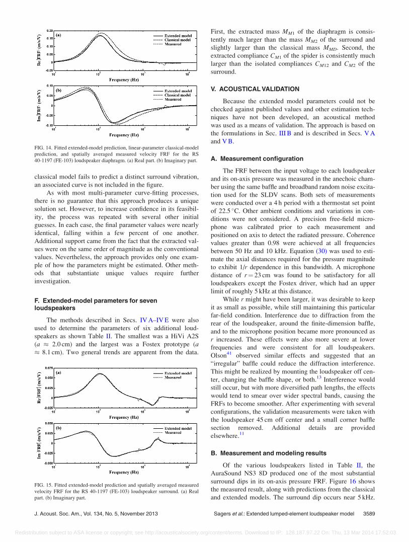
classical model fails to predict a distinct surround vibration,

an associated curve is not included in the figure.

As with most multi-parameter curve-fitting processes,

there is no guarantee that this approach produces a unique

solution set. However, to increase confidence in its feasibil-

ity, the process was repeated with several other initial

guesses. In each case, the final parameter values were nearly

identical, falling within a few percent of one another.

Additional support came from the fact that the extracted val-

ues were on the same order of magnitude as the conventional

values. Nevertheless, the approach provides only one exam-

ple of how the parameters might be estimated. Other meth-

ods that substantiate unique values require further

investigation.

F. Extended-model parameters for sevenloudspeakers

The methods described in Secs. IV A–IV E were also

used to determine the parameters of six additional loud-

speakers as shown Table II. The smallest was a HiVi A2S

(a � 2.0 cm) and the largest was a Fostex prototype (a� 8.1 cm). Two general trends are apparent from the data.

First, the extracted mass MM1 of the diaphragm is consis-

tently much larger than the mass MM2 of the surround and

slightly larger than the classical mass MMD. Second, the

extracted compliance CM1 of the spider is consistently much

larger than the isolated compliances CM12 and CM2 of the

surround.

V. ACOUSTICAL VALIDATION

Because the extended model parameters could not be

checked against published values and other estimation tech-

niques have not been developed, an acoustical method

was used as a means of validation. The approach is based on

the formulations in Sec. III B and is described in Secs. V A

and V B.

A. Measurement configuration

The FRF between the input voltage to each loudspeaker

and its on-axis pressure was measured in the anechoic cham-

ber using the same baffle and broadband random noise excita-

tion used for the SLDV scans. Both sets of measurements

were conducted over a 4 h period with a thermostat set point

of 22.5 C. Other ambient conditions and variations in con-

ditions were not considered. A precision free-field micro-

phone was calibrated prior to each measurement and

positioned on axis to detect the radiated pressure. Coherence

values greater than 0.98 were achieved at all frequencies

between 50 Hz and 10 kHz. Equation (30) was used to esti-

mate the axial distances required for the pressure magnitude

to exhibit 1/r dependence in this bandwidth. A microphone

distance of r¼ 23 cm was found to be satisfactory for all

loudspeakers except the Fostex driver, which had an upper

limit of roughly 5 kHz at this distance.

While r might have been larger, it was desirable to keep

it as small as possible, while still maintaining this particular

far-field condition. Interference due to diffraction from the

rear of the loudspeaker, around the finite-dimension baffle,

and to the microphone position became more pronounced as

r increased. These effects were also more severe at lower

frequencies and were consistent for all loudspeakers.

Olson41 observed similar effects and suggested that an

“irregular” baffle could reduce the diffraction interference.

This might be realized by mounting the loudspeaker off cen-

ter, changing the baffle shape, or both.13 Interference would

still occur, but with more diversified path lengths, the effects

would tend to smear over wider spectral bands, causing the

FRFs to become smoother. After experimenting with several

configurations, the validation measurements were taken with

the loudspeaker 45 cm off center and a small corner baffle

section removed. Additional details are provided

elsewhere.11

B. Measurement and modeling results

Of the various loudspeakers listed in Table II, the

AuraSound NS3 8D produced one of the most substantial

surround dips in its on-axis pressure FRF. Figure 16 shows

the measured result, along with predictions from the classical

and extended models. The surround dip occurs near 5 kHz.

FIG. 14. Fitted extended-model prediction, linear-parameter classical-model

prediction, and spatially averaged measured velocity FRF for the RS

40-1197 (FE-103) loudspeaker diaphragm. (a) Real part. (b) Imaginary part.

FIG. 15. Fitted extended-model prediction and spatially averaged measured

velocity FRF for the RS 40-1197 (FE-103) loudspeaker surround. (a) Real

part. (b) Imaginary part.



While the classical model is not capable of predicting the

anomaly, the extended model predicts it reasonably well. Of

course, neither is able to predict irregularities due to dia-

phragm or surround breakup at higher frequencies. Baffle

diffraction effects are also present in the measured data

while being absent in the modeled FRFs. Nevertheless, the

classical and extended models both produce reasonable

agreement at low frequencies. Only the extended model pro-

vides a useful characterization through the surround dip

region.

Figure 17 shows the measured response of the RS 40-

1197 (FE-103) driver, along with the model predictions. The

extended model successfully predicts the dip near 2 kHz, but

because the measured response is affected by a strong dia-

phragm breakup resonance near 3 kHz (see Fig. 12), it does

not match as well as it might have otherwise. The model

excels at estimating the response magnitude up to the sur-

round resonance frequency f2.

Some loudspeakers did not manifest substantial sur-

round dips (measured or predicted) in their on-axis pressure

FRFs. Although surround resonances were consistently

detected through SLDV scans and resulting SRIFs, their

acoustic effects were sometimes limited, such that the

response dips remained small or negligible. Nevertheless,

the extended model remained successful in the sense that it

accurately predicted these behaviors and consistently pro-

vided better response predictions up to f2.

To better quantify the improvements, linear-scale SSEs

were computed between the predicted and measured on-axis

pressure FRFs for each loudspeaker, with the upper fre-

quency limit set to f2 in each case. The percent reduction in

error between the classical and extended models was subse-

quently calculated as

PRE ¼ 100SSEc � SSEe

SSEc

� �: (34)

The surround resonance frequency, model SSEs, and PRE

are presented in Table III for each loudspeaker. Notable

error reductions occurred in every case, suggesting that the

FIG. 16. Measured and modeled on-axis pressure FRFs for the AuraSound

NS3 8D loudspeaker at r¼ 23 cm.

TABLE II. Conventionally measured parameters and extracted extended-model parameters for seven loudspeakers: (1) HiVi A2S, (2) AuraSound NS3 8D, (3)

Audax HP100MO, (4) RS 40-1197 (FE-103), (5) HiVi M4N, (6) AuraSound NS4 8A, and (7) Fostex prototype.

Loudspeaker number

Parameter 1 2 3 4 5 6 7 Units

a 2.00 3.10 3.90 4.00 4.15 4.20 8.05 cm

b 2.20 3.50 4.35 4.55 4.55 4.60 8.90 cm

Bl 2.97 3.65 5.44 4.65 3.54 3.51 11.2 Tm

CM1 0.000899 0.00145 0.00111 0.00250 0.00240 0.00550 0.00250 m/N

CM2 0.000101 0.00040 0.00030 0.00029 0.00046 0.00038 0.000185 m/N

CM12 0.000202 0.00023 0.00026 0.00053 0.00028 0.00043 0.0000784 m/N

CMS 0.000164 0.00055 0.00042 0.00075 0.00067 0.00089 0.000333 m/N

LE 0.108 0.154 0.173 0.161 0.230 0.165 0.682 mH

MM1 2.82 2.28 6.40 3.00 6.51 3.66 54.5 g

MM2 0.00280 0.00450 0.0170 0.0296 0.00340 0.0327 0.368 g

MMD 2.53 2.11 4.87 2.45 5.43 3.00 39.1 g

RE 6.32 6.76 5.82 7.65 6.48 7.25 6.59 XRM1 0.619 0.339 1.137 0.676 0.483 0.412 0.426 kg/s

RM2 0.232 0.00210 0.257 0.160 0.0330 0.159 3.26 kg/s

RM12 0.0707 0.00490 0.0495 0.0558 0.00100 0.0600 2.31 kg/s

RMS 0.758 0.621 1.08 0.441 0.509 0.432 2.53 kg/s

FIG. 17. Measured and modeled on-axis pressure FRFs for the RS 40-1197

(FE-103) loudspeaker at r¼ 23 cm.



extended model and parameter extraction technique consis-

tently provided better overall predictions of the baffled on-

axis responses than the classical approach.

VI. CONCLUSIONS

This paper has explored a straightforward extension of

the classical lumped-element model of a moving-coil loud-

speaker and demonstrated its potential to improve radiated

acoustic response predictions. It does so by incorporating

additional lumped elements that better represent the distinct

contributions of the diaphragm and surround, while isolating

the roles of the spider and surround in the suspension system.

Experimental results have verified its capabilities for several

baffled loudspeakers from very low frequencies through their

primary and secondary (surround) resonance frequencies. It

extends the effective prediction bandwidth to mid frequen-

cies, while better characterizing loudspeaker responses with

or without notable surround dips. It also provides insights

into their distinctions that may be used to troubleshoot and

improve driver performance characteristics.

Because the model does not predict higher-order inter-

actions and modal behaviors of diaphragms and surrounds,

its benefits are inherently limited. However, it remains a

functional tool that can easily integrate with current loud-

speaker design methods. If properly used, it may assist loud-

speaker designers to better simulate general loudspeaker

responses and systematize alterations to diaphragms, sur-

rounds, and spiders with the aim of improving those

responses. It may also help substantiate the presumed prop-

erties of high or low-quality drivers.

For the model to be successful, its parameters must be

appropriately estimated for a given driver. This paper has

introduced one estimation technique involving the use of

an SLDV to measure velocity frequency response functions

at several diaphragm and surround positions. Their spatial

averages were used with a constrained optimization routine

to estimate the model parameter values. The paper has

introduced an SRIF that easily identifies the surround reso-

nance frequency to help constrain the routine. Other

approaches, including curve fitting of driver electric input

impedances or other measured values, might be explored to

determine the distinct parameters more uniquely. A method

that better predicts the frequency-dependent effective

radiating areas of the diaphragm and surround would also

be beneficial.

The developments have assumed the self and mutual

radiation impedances on the front and back sides of a baffled

loudspeaker are equal. This cannot be strictly true because

the coil former, spider, magnet structure, and frame are not

completely unobtrusive. Moreover, in practical cases, a

driver is mounted on an enclosure with a distinct rear load-

ing. Complete system models must be adapted to these con-

ditions, but if the driver parameters have been successfully

established through initial measurements, system perform-

ance results should be predictable. The authors encourage

research in these and other areas to refine the proposed

model and improve its utility.

LIST OF SYMBOLS

a Radius of a diaphragm, circular piston, inner sur-

round perimeter, or inner annular piston

perimeter

ab Base radius of a right circular cone

aD Effective radius of a diaphragm assembly

b Total radius of a diaphragm and surround, outer

surround perimeter, or outer annular piston

perimeter

Bl Force factor

c Speed of sound in air, � 343 m/s

CMn Effective mechanical compliance of the nth sus-

pension element (extended model)

CMmn Effective mechanical compliance coupling the mth

and nth radiating surfaces (m 6¼ n) (extended

model)

CMS Effective mechanical compliance of the suspen-

sion (classical model)

eg Complex open-circuit voltage amplitude of the

signal generator

F Fitness function for the curve-fitting routine

f Frequency

fn nth resonance frequency of the diaphragm/sur-

round system (n¼ 2 for the surround resonance

frequency)

FRF Frequency response function

GA Acoustic ground (ambient reference

pressure)

Ghs(rjrS) Half-space time-harmonic Green’s function

GM Mechanical ground (zero reference velocity)

h Height of a right circular cone

Hðf Þ Volume velocity FRF (transfer function),

¼ U=eg

H1 First-order Struve function

Hiðf Þ Axial surface velocity FRF (transfer function)

for the ith discrete measurement position,

¼ uSa;i=eg

hs Slant height of a right circular cone

i Integer index value

I Upper limit for ij

ffiffiffiffiffiffiffi�1p

, integer index value

Jn nth-order Bessel function of the first kind

TABLE III. Surround resonance frequencies, sums of squared errors (for the

on-axis response predictions of the classical and extended models), and per-

cent reductions in error (between the two models) for seven loudspeakers:

(1) HiVi A2S, (2) AuraSound NS3 8D, (3) Audax HP100MO, (4) RS 40-

1197 (FE-103), (5) HiVi M4N, (6) AuraSound NS4 8A, and (7) Fostex

prototype.

Loudspeaker number

Measure 1 2 3 4 5 6 7 Units

f2 9105 3920 2310 1670 3430 1680 1440 Hz

SSEc 23.0 22.9 16.8 11.6 1.40 6.70 12.0 Pa2/V2

SSEe 13.1 13.7 1.70 0.60 1.10 1.70 2.40 Pa2/V2

PRE 43.0 40.2 89.9 94.6 21.4 74.6 80.0 %



k Acoustic wave number, ¼ x/cl Index value for discrete measurement

frequencies

LE Effective electric inductance of the voice coil

m Integer index value representing a driver ele-

ment, ¼ 1 or 2

MIFn Mode indicator function for the nth radiating

surface

MMD Effective mechanical mass (classical model)

MMn Effective mechanical mass of the nth radiating

surface (extended model)

n Integer index value representing a driver element, ¼1 or 2 (or 3 for radiation impedance calculations)

nS Unit vector normal to the surface SnS;i Unit vector normal to the surface element DSi

pðrÞ Complex acoustic pressure amplitude at r

pðr; hÞ Axisymmetric complex acoustic pressure ampli-

tude at distance r and angle hpðr; 0Þ On-axis complex acoustic pressure amplitude at

distance rpA;c Complex (spatially averaged) acoustic pressure

amplitude on the back of the diaphragm assem-

bly (classical model)

pA;e Complex (spatially averaged) acoustic pressure

amplitude on the back of the diaphragm

(extended model)

pB;c Complex (spatially averaged) acoustic pressure

amplitude on the front of the diaphragm assem-

bly (classical model)

pB;e Complex (spatially averaged) acoustic pressure

amplitude on the back of the surround (extended

model)

pC;e Complex (spatially averaged) acoustic pressure

amplitude on the front of the diaphragm

(extended model)

pD;e Complex (spatially averaged) acoustic pressure

amplitude on the front of the surround (extended

model)

PRE Percent reduction in error

Qp Directivity factor of a diaphragm assembly along

its principal axis

r Position vector from the origin to the field (ob-

servation) point

r Radial distance from the origin to the field point,

¼ jrjrS Position vector from the origin to a point on a

surface

rS Radial distance from the origin to a point on a

surface, ¼ jrSjR Distance between a surface point and a field

point, ¼ jr 2 rSjRE Electric resistance of the voice coil

RMn Effective mechanical resistance of the nth sus-

pension element (extended model)

RMmn Effective mechanical resistance coupling the mth

and nth radiating surfaces (m 6¼ n) (extended

model)

RMS Effective mechanical resistance of the suspen-

sion (classical model)

S Surface area

SD Effective radiating area of the diaphragm assem-

bly (classical model), ¼ pa2D

Sn Effective area of the nth radiating surface

(extended model)

SRIF Surround resonance indicator function

SSE Sum of the squared error

SSEc Sum of the squared error for the classical model

SSEe Sum of the squared error for the extended

model

U Complex volume velocity amplitude

ui Complex particle velocity amplitude vector,

assumed to be uniform over DSi

uðrSÞ Complex particle velocity amplitude vector at rS

uD Complex normal velocity amplitude of an effec-

tive piston representing the diaphragm assembly

(classical model)

un Complex normal velocity amplitude of the nth

effective piston representing a radiating area of

the diaphragm assembly (extended model)

un;i Complex normal particle velocity amplitude for

the ith discrete measurement position,¼ ui cos hi

uSðrSÞ Complex surface velocity amplitude vector at rS

uSa Complex axial surface velocity amplitude

uSa;i Complex axial surface velocity amplitude for the

ith discrete measurement position

uSnðrSÞ Normal surface velocity amplitude at rS (time

domain)

uSnðrSÞ Complex normal surface velocity amplitude at rS

(frequency domain)

VAS Volume of air having the same acoustic compli-

ance as the driver suspension, ¼ q0c2CMSS2D

VðtÞ Time-varying volume displacement of a dia-

phragm assembly

W Sound power

z Displacement from the (assumed) radiating

plane along the principal loudspeaker axis (coor-

dinate axis)

ZAnn Self-acoustic impedance of the nth radiating sur-

face, modeled as a circular or annular piston in

an infinite plane rigid baffle (extended model)

ZAmn Mutual acoustic impedance between the mth and

nth radiating surfaces (m 6¼ n), modeled as a cir-

cular piston m and a concentric annular piston nin an infinite plane rigid baffle (extended model)

ZAR Acoustic radiation impedance of the diaphragm

assembly, modeled as a circular piston in an in-

finite plane rigid baffle (classical model)

ZE Blocked electric impedance, � REþ jxLE

ZM1 Mechanical impedance substitution (extended

model)


model)


model)

ZMA Mechanical impedance substitution (extended

model)

ZMB Mechanical impedance substitution (extended

model)



ZMC Mechanical impedance substitution (extended

model)

ZMR Mechanical radiation impedance of the dia-

phragm assembly, modeled as a circular piston

in an infinite plane rigid baffle (classical

model)

zSðtÞ Time-varying axial displacement of an idealized

diaphragm surface

a Cone semi-apex angle

c Ratio of radii, ¼ b/aDSi ith discrete surface element

h Angle between r and the axis of a baffled right

circular cone or transformation variable from

Ref. 31

hi Angle between ui and nS,i

k Acoustic wavelength, ¼ c/fq0 Ambient density of air, � 1.21 kg/m3

x Angular frequency, ¼ 2pfh� � �iS Spatial average over the surface Sh� � �iS;w Weighted spatial average over the surface Sh� � �iS;t Spatial and time average over the surface Sh� � �it Time average

1L. L. Beranek, Acoustics (Acoustical Society of America, New York,

1986), pp. 183–188, 191–192, 199–202, 231.2R. H. Small, “Direct-radiator loudspeaker system analysis,” J. Audio Eng.

Soc. 20, 383–395 (1972).3J. N. Moreno, R. A. Moscoso, and S. Jønsson, “Measurement of the effective

radiating surface area of a loudspeaker using a laser velocity transducer and

a microphone,” 96th Conv. Audio Eng. Soc., Preprint 3861 (1994).4W. Klippel and J. Schlechter, “Dynamic measurement of transducer effec-

tive radiation area,” J. Audio Eng. Soc. 59, 44–52 (2011).5H. F. Olson, J. Preston, and E. G. May, “Recent developments in direct-

radiator high-fidelity loudspeakers,” J. Audio Eng. Soc. 2, 219–227 (1954).6J. Eargle, Loudspeaker Handbook, 2nd ed. (Kluwer, Boston, 2003), pp.

30–31.7P. Newell and K. Holland, “Diversity of design: Loudspeakers by Philip

Newell and Keith Holland,” in Audio Engineering Explained—Professional Audio Recording, edited by D. Self (Focal Press, Oxford,

2010), Chap. 12, pp. 357–358.8T. W. Leishman and J. Tichy, “A theoretical and numerical analysis of

vibration-controlled modules for use in active segmented partitions,”

J. Acoust. Soc. Am. 118, 1424–1438 (2005).9J. D. Sagers, T. W. Leishman, and J. D. Blotter, “A double-panel active

segmented partition module using decoupled analog feedback controllers:

Numerical model,” J. Acoust. Soc. Am. 125, 3806–3818 (2009).10R. J. True, “The dominant compliance of loudspeaker drivers,” SAE

International Congress and Exposition, Detroit, SAE Technical Paper

910651 (1991).11J. D. Sagers, “Analog Feedback Control of an Active Sound Transmission

Control Module,” M.S. thesis, Brigham Young University, Provo, UT

(2008), Chap. 4. Available online through Brigham Young University

Electronic Theses & Dissertations at <http://etd.lib.byu.edu> (Last

viewed July 5, 2013).12J. D. Sagers, T. W. Leishman, and J. D. Blotter, “Active sound transmission

control of a double-panel module using decoupled analog feedback control:

Experimental results,” J. Acoust. Soc. Am. 128, 2807–2816 (2010).13IEC 60268-5, Sound System Equipment—Part 5: Loudspeakers, 3rd ed.

(International Electrotechnical Commission, Geneva, Switzerland, 2003).14F. J. M. Frankort, “Patterns and radiation behavior of loudspeaker cones,”

J. Audio Eng. Soc. 26, 609–622 (1978).

15T. Shindo, O. Yashima, and H. Suzuki, “Effect of voice-coil and surround

on vibration and sound pressure response of loudspeaker cones,” J. Audio

Eng. Soc. 28, 490–499 (1980).16D. A. Barlow, G. D. Galletly, and J. Mistry, “The resonances of loud-

speaker diaphragms,” J. Audio Eng. Soc. 29, 699–704 (1980).17M. S. Corrington and M. C. Kidd, “Amplitude and phase measurements

on loudspeaker cones,” Proc. IRE 39, 1021–1026 (1951).18K. Suzuki and I. Nomoto, “Computerized analysis and observation of the vibra-

tion modes of a loudspeaker cone,” J. Audio Eng. Soc. 30, 98–106 (1982).19W. M. Leach, Jr., Introduction to Electroacoustics and Audio Amplifier

Design, 4th ed. (Kendall Hunt, Dubuque, IA, 2010), pp. 89–94.20J. A. D’Appolito, Testing Loudspeakers (Audio Amateur Press,

Peterborough, NH, 1998), Chaps. 2, 3, and 7.21L. L. Beranek and T. J. Mellow, Acoustics: Sound Fields and Transducers

(Academic Press, London, 2012), Sec. 4.16, Chap. 6.22A. D. Pierce, Acoustics: An Introduction to its Physical Principles and

Applications (Acoustical Society of America, New York, 1989), Secs. 4–6

and 5–2, pp. 320–321.23E. G. Williams, Fourier Acoustics: Sound Radiation and Nearfield

Acoustical Holography (Academic Press, London, 1999), Sec. 2.10, Chap. 8.24W. N. Brown, Jr., “Theory of conical sound radiators,” J. Acoust. Soc.

Am. 13, 20–22 (1941).25P. G. Bordoni, “The conical sound source,” J. Acoust. Soc. Am. 17,

123–126 (1945).26F. J. M. Frankort, “Vibration and sound radiation of loudspeaker cones,”

Ph.D. dissertation, Delft University of Technology, Delft, The

Netherlands (1975) [reprinted in Philips Res. Rep., Suppl. No. 2, pp.

1–189 (1975)], pp. 110–125.27L. E. Kinsler, A. R. Frey, A. B. Coppens, and J. V. Sanders, Fundamentals

of Acoustics, 4th ed. (Wiley, New York, 2000), pp. 179–181, 186.28D. K. Anthony and S. J. Elliott, “A comparison of three methods of meas-

uring the volume velocity of an acoustic source,” J. Audio Eng. Soc. 39,

355–366 (1991).29S. Jønsson, “Accurate determination of loudspeaker parameters using

audio analyzer type 2012 and laser velocity transducer type 3544,” Br€uel

and Kjær Application Note BO 0384-12 (1996).30C. H. Hansen and S. D. Snyder, Active Control of Noise and Vibration

(E & FN Spon, London, 1997), pp. 117–118.31P. R. Stepanishen, “The impulse response and mutual radiation impedance

between a circular piston and a piston of arbitrary shape,” J. Acoust. Soc.

Am. 54, 746–754 (1973).32P. R. Stepanishen, “Impulse response and radiation impedance of an annu-

lar piston,” J. Acoust. Soc. Am. 56, 305–312 (1974).33P. R. Stepanishen, “Evaluation of mutual radiation impedances between

circular pistons by impulse response and asymptotic methods,” J. Sound

Vib. 59, 221–235 (1978).34W. Thompson, Jr., “The computation of self- and mutual-radiation impe-

dances for annular and elliptical pistons using Bouwkamp’s integral,”

J. Sound Vib. 17, 221–233 (1971).35W. Klippel and J. Schlechter, “Distributed mechanical parameters of

loudspeakers, Part 1: Measurements,” J. Audio Eng. Soc. 57, 500–511

(2009).36T. W. Leishman, “Active control of sound transmission through partitions

composed of discretely controlled modules,” Ph.D. thesis, The

Pennsylvania State University (2000), Chap. 7.37T. W. Leishman and J. Tichy, “An experimental investigation of two mod-

ule configurations for use in active segmented partitions,” J. Acoust. Soc.

Am. 118, 1439–1451 (2005).38P. L. Gatti and V. Ferrari, Applied Mechanical and Structural Vibrations:

Theory, Methods, and Measuring Instrumentation (E & FN Spon, London,

1999), p. 461.39P. Avitabile, “Modal space: What is the difference between all the mode

indicator functions? What do they all do?,” Exp. Tech. 31, 15–16 (2007).40M. H. Richardson, “Is it a mode shape, or an operating deflection shape?,”

Sound Vib. 31, 54–61 (1997).41H. F. Olson, Acoustical Engineering (Professional Audio Journals,

Philadelphia, 1991), Sec. 6.8.



http://etd.lib.byu.edu

an extended lumped-element model and parameter estimation ...€¦ · an extended lumped-element...

Documents