an extension of erlang distribution with properties having

Int. J. Open Problems Compt. Math., Vol. 14, No. 1, March 2021

Print ISSN: 1998-6262, Online ISSN: 2079-0376

Copyright @ICSRS Publication, 2021, www.i-csrs.org

An Extension of Erlang Distribution with

Properties Having Applications In

Engineering and Medical-Science

Ahmad Aijaz1, S. Qurat ul Ain2, Afaq Ahmad3, and Rajnee Tripathi4

1,2,4 Department of Mathematics, Bhagwant University, Ajmer, Rajasthan, India

3Department of Mathematical Sciences, Islamic University of Science

& Technology, Awantipora, Kashmir3

e-mail: [email protected]

Abstract

In this work an extension of Erlang distribution have been introduced,

which is in fact a generalization of Erlang distribution. This

generalization is derived by applying power transformation technique

and it gives more flexibility to investigate complex real life data. The

distinct structural properties of the formulated distribution including

moments, moment generating function, skewness, kurtosis, incomplete

moments, mode, median, order statistics, different measure of

entropies, mean deviations, Bonferroni and Lorenz curves have been

discussed. In addition expressions for survival function, hazard rate

function, reverse hazard rate function and mean residual function are

obtained explicitly. The behaviour of probability density function

(p.d.f) and cumulative distribution function (c.d.f) are illustrated

through different graphs. The estimation of the established distribution

parameters are performed by maximum likelihood estimation method.

Eventually the versatility of the established distribution is examined

through two real life data sets related to engineering and medical

science.

Key words:- Erlang distribution, power transformation technique, moments,

entropies, reliability measures, maximum likelihood estimation.

Mathematics subject classification: 60-XX, 62-XX, 11-KXX

mailto:[email protected]

An Extension Of Erlang Distribution… 47

1 Introduction

Analysing or modelling of complex real life data collected from different fields of

science like bio-medicine, engineering, actuarial science and environment is

challenging among researchers. In these situations an emergence of new

distributions or modifications of the existing distributions become need of an hour.

In the literature of statistics there exist various methods to address these problems.

Power transformation of probability distributions is one of the known technique by

which an extra parameter is added to the parent distribution. The resulting

distributions obtained after applying different methods become richer or more

flexible for analysing diverse data. Erlang distribution is one of the popular

continuous probability distribution having following probability density function.

xexxf

1),,( ,...3,2,1,0,0; x 1.1

The corresponding distribution function is given by

x

xF,

,, ,...3,2,1,0,0; x 2.1

It was established by A.K. Erlang [6] to examine the number of telephone calls

which are received simultaneously to the operators of the switching stations. This

distribution has since been extended for use in queuing theory, the mathematical

study of waiting in lines. Erlang’s distribution has also vast applications in

mathematical biology and stochastic process. Due to vast applications of Erlang

distribution researcher have made lot of work to improve this distribution. Haq and

Dey [8] have studied the Bayes analysis of the Erlang distribution and used different

informative priors. Bhattacharya and Singh [5] obtained a Bayes estimator for the

Erlangian que based on two prior distributions. Khan and Jan [11] used various

generalized truncated prior distribution to discuss and obtain estimates for the

Erlang distribution. Sofi Mudasir at el [14] proposed and studied characterization

and information measures of weighted Erlang distribution. Hesham at el [9]

introduced Length-biased weighted Erlang distribution also they discussed its

various properties. Sofi Mudasir at el [15] used different priors to obtain parameter

estimation of weighted Erlang distribution. They used R software and expounded

the performance of the distribution through real life data set. In this paper we

generalize Erlang distribution by power transformation approach. This technique

has attracted the attention of researchers from past decade due to which several

Ahmad Aijaz, S. Qurat ul Ain, Afaq Ahmad, and Rajnee Tripathi 48

papers has come into existence. Ghitany et al [7] established power Lindley

distribution and elaborate its several structural properties. Krishnarani [12] used

power transformation method on Half – Logistic distribution and studied its

different characteristics. Rady et al [18] introduced power Lomax distribution, then

the resulting distribution and applied it on medical related data set. Shukla et al [16]

proposed and examine the performance of power Ishita distribution. A. A. Bhat et

al [1] studied and formulated a new generalization of Rayleigh distribution by

applying the power transformation method.

2 Power Erlang Distribution

Let us suppose X be a random variable follows probability density function 1.1 ,

then the transformation

1

XY is said to follow power Erlang distribution denoted

as ,,~ PErDY if its probability density function (p.d.f) is give as

yeyyf

1,,, ,...3,2,1,0,;0; y 1.2

Figure (1.1) and (1.2), illustrates the behaviour of the p.d.f of power Erlang

distribution for varying values of the parameters.

The corresponding cumulative distribution function (c.d.f) is given by


yyF

,,,, ,...3,2,1,0,;0; y 2.2

Figure (2.1) and (2.2), illustrates the behaviour of the c.d.f of power Erlang

distribution for varying values of the parameters.

3 Reliability Analysis

SupposeY be a continuous random variable with c.d.f yF , 0y .Then its

reliability function which is also called survival function is defined as

yFdyyfyYpySy

r

1

Therefore, the survival function for power Erlang distribution is given as

,,,1,,, yFyS

y,1 1.3


Figure (3.1) and (3.2), illustrates the behaviour of the survival function of power

Erlang distribution for varying values of the parameters.

The hazard rate function of a random variable y is given as

,,,

,,,,,,

yS

yfyH 2.3

Using equation 1.2 and equation 1.3 in 2.3 , we get

y

eyyH

y

,,,,

1

Figure (4.1) and (4.2), illustrates the behaviour of the hazard rate function of power

Erlang distribution for varying values of the parameters.


Reverse hazard rate function of random variable y is given by

,,,

,,,,,,

yF

yfyhr 3.3

Using equation 1.2 and equation 2.2 in 3.3 , we get

y

eyyh

y

r,

..,1

Figure (5.1) and (5.2), illustrates the behaviour of the reverse hazard rate function

of power Erlang distribution for varying values of the parameters.

Mean residual function of random variable y can be obtained as

ydtttfyS

ymy

,,,,,,

1,,,

ydtett

y

y

1

,,

y

y ydtety

,

After solving the integral, we get


yy

y

ym

,

,1

,,,

1

4 Mathematical Properties Power Erlang Distribution

4.1 Moments of power Erlang distribution

Let Y be a random variable follows power Erlang distribution. Then thr moment

denoted by '

r is given as

dyyfyYE rr

r

0

' ,,,

dyeyy yr

1

0

dyey yr

0

1

Making substitution zy and z0 , we have

dzez z

r

r

0

1'

rr

r

'

Now substituting 4,3,2,1r we obtain first four moments about origin of power

Erlang distribution

1

'

1

1

,

2

'

2

2


3

'

3

3

,

4

'

4

4

The moments about mean of the power Erlang distribution are obtained by using

relationship between moments about mean and moments about origin

22

2

2

)(

12

33

3

2

3

12

23

3

44

42

23

4

13

126

134

4

The standard deviation (S.D), coefficient of variation (c.v), coefficient of skewness

1 , coefficient of kurtosis 2 , index of dispersion of power Erlang

distribution are determined as

)(

12

1

2

1

12

.

2

'

1

VC


2

3

2

2

3

2

31

12

12

23

3

22

42

23

2

2

41

12

13

126

134

4

1

12

1

2

'

1

2

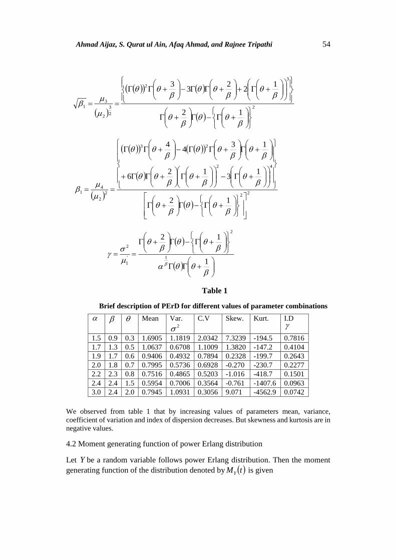
Table 1

Brief description of PErD for different values of parameter combinations

We observed from table 1 that by increasing values of parameters mean, variance,

coefficient of variation and index of dispersion decreases. But skewness and kurtosis are in

negative values.

4.2 Moment generating function of power Erlang distribution

Let Y be a random variable follows power Erlang distribution. Then the moment

generating function of the distribution denoted by tMY is given

Mean Var. 2

C.V

Skew. Kurt. I.D

1.5 0.9 0.3 1.6905 1.1819 2.0342 7.3239 -194.5 0.7816

1.7 1.3 0.5 1.0637 0.6708 1.1009 1.3820 -147.2 0.4104

1.9 1.7 0.6 0.9406 0.4932 0.7894 0.2328 -199.7 0.2643

2.0 1.8 0.7 0.7995 0.5736 0.6928 -0.270 -230.7 0.2277

2.2 2.3 0.8 0.7516 0.4865 0.5203 -1.016 -418.7 0.1501

2.4 2.4 1.5 0.5954 0.7006 0.3564 -0.761 -1407.6 0.0963

3.0 2.4 2.0 0.7945 1.0931 0.3056 9.071 -4562.9 0.0742


dyyfeeEtM tyty

Y

0

,,,

Using Taylor’s series

dyyf

tytyty ,,,...

!3!21

0

32

dyyfyr

t r

r

r

00

,,,!

r

r

r

YEr

t

0 !

r

r

r

Y

r

r

ttM

0 !

4.3 Characteristics function of power Erlang distribution

Let Y be a random variable follows power Erlang distribution. Then the

characteristics function of the distribution denoted by tY is given

dyyfeeEt ityity

Y

0

,,,

Using Taylor’s series

dyyf

ityityity ,,,...

!3!21

0

32

dyyfyr

it r

r

r

00

,,,!

)(

r

r

r

YEr

it

0 !

)(


r

r

r

Y

r

r

itt

0 !

)(

4.4 Incomplete moments of power Erlang distribution

The qth incomplete moment of power Erlang distribution about origin is given by

dyyfysT

s

s

q ,,,0

s

ys dyey0

1

Making substitution zy and sz 0 , we have

dzezsT z

s ss

q

0

1

s

ssT

s

q ,

4.5 Harmonic mean of power Erlang distribution

The harmonic mean of power Erlang distribution is given by

dyyfyY

EH

,,,111

0

dyeyy

y

1

0

1

dyey y

0

2

Making substitution zy , we have


dzezH

z

0

11

1

1

1

4.6 Mode and median of power Erlang distribution

Taking logarithm of equation 1.2 , we have

yyyf log1logloglog,,,log

1.4 Differentiate equation 1.4 , with respect to y , we obtain

11,,,log

yyy

yf

Substituting

0,,,log

y

yf , we get

2

1

00

2

1

11

yMy

Using the empirical formula for median, we get

'

103

2

3

1 MM d

1

2

11

21

3

1dM

5 Shanon’s Entropy Of Power Erlang Distribution

The notion of entropy was introduced by Shanon in 1948. The entropy can be

interpreted as the average rate at which information is produced by a random source

of data and is given as


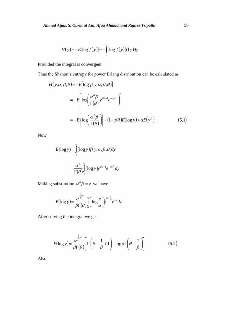
dyyfyfyfEyH

0

loglog

Provided the integral is convergent

Thus the Shanon’s entropy for power Erlang distribution can be calculated as

,,,log,,, yfEyH

yeyE 1log

yEyEE

log1log 1.5

Now

dyyfyyE ,,,log)(log0

dyeyy y

1

0

log

Making substitution z we have

dzezz

yE z

1

0

11

loglog

After solving the integral we get

1log1

1log '

11

yE 2.5

Also


dyeyyE y

0

11

Making substitution zy , we get

dzezyE z

0


1yE 3.5

Using equation 2.5 , 3.5 in equation 1.5 , we get

1

log11

1log,,,

'

1

yH

6 Renyi Entropy Of Power Erlang Distribution

If Y is a continuous random variable having probability density function

,,,yf . Then

Renyi entropy is defined as

0

log1

1dyyfTR

, where 0 and 1

Thus, the Renyi entropy for power Erlang distribution 1.2 , is given as

0

1log1

1dyeyT y

R

0

)1(log1

1dyey y

Making substitution zy , we have


dzezT z

R

0

1111

log1

1


11

1 11log

1

1

RT

11log1

1 11

RT

7 Mathai and Haubold Entropy of Erlang Distribution

The measure of entropy given by Mathai and Haubold is defined as

0

2log1

1dyyfTMH

, where 0 and 1

Thus, the Mathai and Haubold entropy for power Erlang distribution 1.2 , is given

as

0

2

1log1

1dyeyT y

MH

0

)2()2)(1(

2

log1

1dyey y


1)2(1log1

12

1)2(1

MHT

8 Tsallis Entropy of Power Erlang Distribution

Tsallis entropy of order for power Erlang distribution 1.2 , is given as


0

11

1dyyfS

, where 0 and 1

0

111

1dyeyS y


1111

1 11

S

9 Mean Deviation From Mean of Power Erlang

Distribution

The quantity of scattering in a population is evidently measured to some extent by

the totality of the deviations. Let Y be a random variable from power Erlang

distribution with mean .Then the mean deviation from mean is defined as.

YED

dyyfY

0

dyyfydyyfy

0

dyyfdyyyfdyyyfdyyf

00

dyyyfFdyyyfF

10

dyyyfF

0

22 1.9

Now


dyeyydyyyf y

1

00

0

dyey y

Making the substation zy ,

1

0 z , we have

dzez z

1

0

1111


111

0

,1

dyyyf 2.9

Using equation 2.9 in equation 1.9 , we have

1

11 ,1

,2

D

10 Mean Deviation From Median of Power Erlang

Distribution

Let Y be a random variable from power Erlang distribution with median M .Then

the mean deviation from median is defined as.

MYEMD

dyyfMY

0

dyyfMydyyfyMM

M

0

dyyyfMFMdyyyfMMFM

M

10


dyyyf

M

0

2 1.10

Now

dyeyydyyyf y

MM

1

00

M

y dyey0

Making the substation zy ,

1

0 Mz , we have

dzez z

M

1

0

1111


111

0

,1

Mdyyyf

M

2.10

Using equation 2.10 in equation 1.10 , we have

111

,1

2 MMD

11 Bonferroni and Lorenz Curves

In economics the relation between poverty and economy is well studied by

using Bonferroni and Lorenz curves. Besides that these curves have been used

in different fields such as reliability, insurance and biomedicine.

The Bonferroni curves, sB is given as

dyyyfs

sB

t

0

1

1.11

Or


dyyFs

sB

s

0

11

And Lorenz curves, sL is given as

dyyyfsL

t

0

1

2.11

Or

dyyFsL

s

0

11

Where XE and sFt 1

Now

dyeyydyyyf y

tt

1

00

dyey

t

y

0


111

0

,1

tdyyyf

t

3.11

Substituting equation 3.11 in equations 1.11 and 2.11 , we get

And

111

,1

ts

sB

111

,1

tsL


12 Order Statistics of Power Erlang Distribution

Let nYYYY ,....,,, 321 denotes the order statistics of a random sample drawn

from power a continuous distribution with cdf yF and pdf yf , then the pdf

of kY is given by

kn

Y

k

YYkY yFyFyfknk

nYf

1

!!1

!,

1 nk ....,3,2,1 1.12

Substitute the equation 1.2 and 2.2 in equation 1.12 , we obtain the

probability function of thk order statistics of power Erlang distribution is given

by

knk

kY

yyy

knk

nYf

,1

,

!!1

!,

1

1 1.12

Then, the pdf of first order 1Y power Erlang distribution given by

k

Y

yy

nYf

1

1

1

,1,

And the pdf of nth order nY power Erlang distribution is given by

1

1 ,,

n

nY

yy

nYf

13 Maximum Likelihood Estimator Of Power Erlang

Distribution

Let nYYY ,..,, 21 be a random sample of size n from power Erlang distribution then its

likelihood function is given by

n

i

iyfl1

,,,

n

i

iyn

i

ey 1

1

1


n

i

iyn

i

i

n

ey 1

1

1

The log likelihood function becomes

n

i

i

n

i

i yynnnl11

log1loglogloglog

1.13

Differentiating 1.13 w.r.t the parameters, we get

n

i

iynl

1

log

n

i

ii

n

i

i yyynl

11

loglog

n

i

iynnl

1

logloglog

Where

'

The above equations are non-linear equations which cannot be expressed in

compact form and it is difficult to solve these equations explicitly for , and

.Applying the iterative methods such as Newton–Raphson method, secant method,

Regula-falsi method etc. The MLE of the parameters denoted as ˆ,ˆ,ˆˆ of

,, can be obtained by using the above methods.

Since the MLE of follows asymptotically normal distribution which is given as

INn ,0ˆ

Where 1I is the limiting variance-covariance matrix and I is a 33

Fisher information matrix

i,e


2

222

2

2

22

22

2

2

logloglog

logloglog

logloglog

1

lE

lE

lE

lE

lE

lE

lE

lE

lE

nI

Where

22

2 log

nl

; 2

122

2

loglog

i

n

i

i yynl

;

'

2

2 logn

l

n

i

ii yyll

1

22

logloglog

nll

loglog 22

n

i

iyll

1

22

logloglog

Hence the approximate %1100 confidence interval for , and are

respectively given by

ˆˆ 1

2

IZ

ˆˆ, 1

2

IZ and ˆˆ 1

2

IZ

Where 2

Z is the th percentile of the standard distribution.

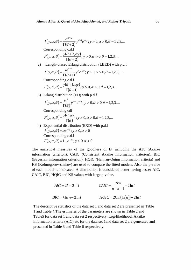
14 Applications

In this section the versatility of the formulated distribution is examined through two

data sets which are related different fields of science. To examine the significance

and potentiality of the formulated distribution, we compare the formulated

distribution with its sub models having following densities.

1) Area-biased Erlang distribution (ABED) with p.d.f


,...3,2,1,0,0;2

,, 12

yeyyf y

Corresponding c.d.f

,...3,2,1,0,0;2

,2,,

y

yyF

2) Length-biased Erlang distribution (LBED) with p.d.f

,...3,2,1,0,0;1

,,1

yeyyf y

Corresponding c.d.f

,...3,2,1,0,0;1

,1,,

y

yyF

3) Erlang distribution (ED) with p.d.f

,...3,2,1,0,0;,, 1

yeyyf y

Corresponding cdf

,...3,2,1,0,0;,

,,

y

yyF

4) Exponential distribution (EXD) with p.d.f

0,0;,, yeyf y

Corresponding c.d.f

0,0;1,, yeyF y

The analytical measures of the goodness of fit including the AIC (Akaike

information criterion), CAIC (Consistent Akaike information criterion), BIC

(Bayesian information criterion), HQIC (Hannan-Quinn information criteria) and

KS (Kolmogorov-smirov) are used to compare the fitted models. Also the p-value

of each model is indicated. A distribution is considered better having lesser AIC,

CAIC, BIC, HQIC and KS values with large p-value.

lkAIC ln22 lkn

knCAIC ln2

1

2

lnkBIC ln2ln lnkHQIC ln2lnln2

The descriptive statistics of the data set 1 and data set 2 are presented in Table

1 and Table 4.The estimates of the parameters are shown in Table 2 and

Table5 for data set 1 and data set 2 respectively. Log-likelihood, Akaike

information criteria (AIC) etc for the data set 1and data set 2 are generated and

presented in Table 3 and Table 6 respectively.


Data Set 1:- The following data represent 40 patients suffering from blood

cancer (leukaemia) from one ministry of health hospitals in Saudi Arabia (see

Abouammah et al.). The ordered lifetimes (in years) are given.

0.315, 0.496, 0.616, 1.145, 1.208, 1.263, 1.414, 2.025, 2.036, 2.162,

2.211, 2.37, 2.532, 2.693, 2.805, 2.91, 2.912, 3.192, 3.263, 3.348, 3.348,

3.427, 3.499, 3.534, 3.767, 3.751, 3.858, 3.986, 4.049, 4.244, 4.323, 4.381,

4.392, 4.397, 4.647, 4.753, 4.929, 4.973, 5.074, 5.381

Table 2

The descriptive statistics of data set 1 of 40 patients suffering from

leukaemia

Min Q1 Q3 Mean Median Skew. Kurt. Max

0.315 2.199 4.264 3.141 3.348 -0.41 2.273 5.381

Table 3

The ML Estimates of the unknown parameters for Data set 1st

Table 4

Performance of distributions for Data set 1st

Model llog2 AIC CAIC BIC HQIC K-S P-

value

PED 135.171 141.171 141.838 146.238 143.003 0.115 0.659

ABED 147.096 151.097 151.421 154.475 152.318 0.158 0.269

LBED 147.096 151.097 151.421 154.475 152.318 0.158 0.269

ED 147.096 151.097 151.497 154.475 152.104 0.637 4.6e-

12

EXD 171.556 173.556 173.685 175.245 174.059 0.599 9.6e-11

Data Set 2: The data represents the breaking stress of carbon fibres of 50mm

length (GPa) and has been already used by Al-Aqtash et al. [3] demonstrate the

appropriateness of Gumbell-Weibull distribution. The data set is follows

Model S.E

PED 0.0036 3.803 0.5265 0.0019 0.336 0.099

ABED 1.1031 …… 1.4647 0.2537 …… 0.7404

LBED 1.4647 …… 2.4647 0.2537 …… 0.2537

ED 1.1031 ……. 3.4647 0.2537 …… 0.7404

EXD 0.3183 ……. …… 0.0503 ……. …….


0.39, 0.85, 1.08, 1.25, 1.47, 1.57, 1.61, 1.61, 1.69, 1.80, 1.84, 1.87, 1.89, 2.03,

2.03, 2.05, 2.12, 2.35, 2.41, 2.43, 2.48, 2.50, 2.53, 2.55, 2.55, 2.56, 2.59, 2.67,

2.73, 2.74, 2.79,2.81, 2.82, 2.85, 2.87, 2.88, 2.93, 2.95, 2.96, 2.97, 3.09, 3.11,

3.11, 3.15, 3.15, 3.19, 3.22, 3.22, 3.27, 3.28, 3.31, 3.31, 3.33, 3.39, 3.39, 3.56,

3.60, 3.65,3.68, 3.70, 3.75, 4.20, 4.38, 4.42, 4.70, 4.90

Table 5

The descriptive statistics of data set 2 of breaking stress of carbon fibres

Min Q1 Q3 Mean Median Skew. Kurt. Max

0.390 2.178 3.277 2.760 2.835 -0.13 3.223 4.90

Table 6

The ML Estimates of the unknown parameters for Data set 2nd

Table 7

Performance of distributions for Data set 2nd

Model llog2 AIC CAIC BIC HQIC K-S P-

value

PED 171.8988 177.898 178.286 184.467 180.494 0.083 0.751

ABED 182.334 186.335 186.525 190.714 188.065 0.132 0.194

LBED 182.334 186.335 186.525 190.714 188.065 0.132 0.194

ED 182.334 186.335 186.525 190.714 188.065 0.703 1.3e-

14

EXD 265.988 267.988 268.117 270.178 268.492 0.603 7.5e-

11

Since it has been observed from table 4 and table 7 that the power Erlang distribution

has smaller values for the AIC, AICC, CAIC, BIC, HQIC and K-S statistics as

Model S.E

PED 0.012

2

3.761

7

0.856

7

0.013

3

0.666

5

0.251

5

ABE

D

2.713

5 …… 5.488

0

0.478

0 …… 1.275

5

LBED 2.713

5 …… 6.488

0

0.478

0 …… 1.275

5

ED 2.713

5 ……. 7.488

0

0.478

0 …… 1.275

5

EXD 0.362

3 ……. …… 0.044 ……. …….


compared with its sub models. Accordingly we arrive the conclusion that power

Erlang distribution provides an adequate fit than compared ones.

Figure (1.1) and (1.2) represents the estimated densities of the fitted distributions to

data set 1st and 2nd.

15 Conclusion

This paper introduces an extension of Erlang distribution which is obtained by

applying power transformation method. For this distribution several

mathematical quantities are derived including moments, moment generating

function, skewness, kurtosis, incomplete moments, mode, median, order

statistics, different measure of entropies, mean deviations, Bonferroni and

Lorenz curves. An account on reliability analysis has been discussed. Different

plots have been drawn to show the behaviour of p.d.f, c.d.f and other related

measures. The method of maximum likelihood estimation has been applied for

estimating the parameters of the distribution. Lastly it has been carried out

through two real life data sets that the formulated distribution leads an

improved fit than compared ones.

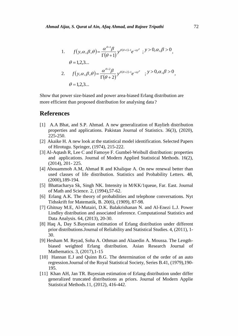
16 Open Questions

The following probability density function represents power size-biased and

power area-biased Erlang distribution.


1.

yeyyf

11

1

1,,, ; 0,,0 y ,

...3,2,1

2.

yeyyf

12

2

2,,,

; 0,,0 y ,

...3,2,1

Show that power size-biased and power area-biased Erlang distribution are

more efficient than proposed distribution for analysing data ?

References

[1] A.A Bhat, and S.P. Ahmad. A new generalization of Raylieh distribution

properties and applications. Pakistan Journal of Statistics. 36(3), (2020),

225-250.

[2] Akaike H. A new look at the statistical model identification. Selected Papers

of Hirotugu. Springer, (1974), 215-222.

[3] Al-Aqtash R, Lee C and Famoye F. Gumbel-Weibull distribution: properties

and applications. Journal of Modern Applied Statistical Methods. 16(2),

(2014), 201- 225.

[4] Abouammoh A.M, Ahmad R and Khalique A. On new renewal better than

used classes of life distribution. Statistics and Probability Letters. 48,

(2000),189-194.

[5] Bhattacharya Sk, Singh NK. Intensity in M/KK/1queue, Far. East. Journal

of Math and Science. 2, (1994),57-62.

[6] Erlang A.K. The theory of probabilities and telephone conversations. Nyt

Tidsskrift for Matematik, B. 20(6), (1909), 87-98.

[7] Ghitnay M.E, Al-Mutairi, D.K. Balakrishanan N. and Al-Enezi L.J. Power

Lindley distribution and associated inference. Computational Statistics and

Data Analysis. 64, (2013), 20-30.

[8] Haq A, Day S.Bayesian estimation of Erlang distribution under different

prior distributions.Journal of Reliability and Statistical Studies. 4, (2011), 1-

30.

[9] Hesham M. Reyad, Soha A. Othman and Alaaedin A. Moussa. The Length-

biased weighted Erlang distribution. Asian Research Journal of

Mathematics. 3, (2017),1-15

[10] Hannan E.J and Quinn B.G. The determination of the order of an auto

regression.Journal of the Royal Statistical Society, Series B.41, (1979),190-

195.

[11] Khan AH, Jan TR. Bayesian estimation of Erlang distribution under differ

generalized truncated distributions as priors. Journal of Modern Applie

Statistical Methods.11, (2012), 416-442.


[12] Krishnarani S.D. On a power transformation of Half-Logistic distribution.

Journal of Probability and Statistics. 5, (2016), 1-10.

[13] Mathai A.M and Haubold H.J (2007). Pathway model, Super statistics,

Tsallis Statistics and generalized measures of entropy. Physica A: Statistical

Mechanics and its Applications. 375(1), (2016),110-1212.

[14] Sofi Mudasir and S.P .Ahmad. Characterization and information measures

of weighted Erlang distribution. Journal of Statistics Applications and

Probability Letters. 4(3), (2017), 109-122.

[16] Sofi Mudasir and S.P .Ahmad. Parameter estimation of weighted Erlang

distribution using R software. Mathematical theory and Modelling. 7(6),

(2017), 1- 21.

[17] Shukla K.K and Shanker R (2018). Power Ishita distribution and its

application to model lifetime data. Statistics in Transition. 19(1), (2017),

135-148.

[18] Shanon E. A mathematical theory of communication. Bell System

Technical Journal. 27(3), (1948),379-423.

[19] Rady E.H.A, Hassanien W.A and Elhaddad T.A. The power Lomax

distribution with an application to bladder cancer data. Springer Plus. 5,

(2016).

[21] Renyi A. On measures of entropy and information. Berkeley Symposium

on Mathematical Statistics and Probability. 1(1), (1960),547-561.

[22] Zaka A and Akhtar A.S. Methods for estimating the parameters of power

Function distribution. Pakistan Journal of Statistics and Operation

Research.9, (2013), 213-224.

an extension of erlang distribution with properties having

Documents