an extension of the basic theorems of classical welfare

AN EXTENSION OF THE BASICTHEOREMS OF CLASSICALWELFARE ECONOMICS

KENNETH J. ARROWSTANFORD UNIVERSITY

1. SummaryThe classical theorem of welfare economics on the relation between the price

system and the achievement of optimal economic welfare is reviewed from theviewpoint of convex set theory. It is found that the theorem can be extended tocover the cases where the social optima are of the nature of corner maxima, and alsowhere there are points of saturation in the preference fields of the members of thesociety. The first point is related to an item in the Hicks-Kuznets discussion of realnational income. The assumptions underlying the analysis are briefly reviewed andcriticized.

I wish to thank Gerard Debreu, Cowles Commission for Research in Economics,for helpful comments.

2. IntroductionIn regard to the distribution of a fixed stock of goods among a number of indi-

viduals, classical welfare economics asserts that a necessary and sufficient condi-tion for the distribution to be optimal (in the sense that no other distribution willmake everyone better off, according to his utility scale) is that the marginal rate ofsubstitution between any two commodities be the same for every individual.'Similarly, a necessary and sufficient condition for optimal production from givenresources (in the sense that no other organization of production will yield greaterquantities of every commodity) is stated to be that the marginal rate of transfor-mation for every pair of commodities be the same for all firms in the economy.2

Let it be assumed that for each consumer and each firm there is no divergencebetween social and private benefits or costs, that is, a given act of consumption orproduction yields neither satisfaction nor loss to any member of the society other

This article will be reprinted as Cowles Commission Paper, New Series, No. 54.1 By marginal rate of substitution between any commodity A and commodity B is meant the

additional amount of commodity A needed to keep an individual as well off as he was before losingone unit of B, the amounts of all other commodities being held constant. If the preference scale forcommodity bundles is expressed by means of a utility indicator, then the marginal rate of substitu-tion between A and B equals the marginal utility of A divided by the marginal utility of B. See,for example, [8, pp. 19-20].

2 The marginal rate of transformation between commodities A and B is the amount by whichthe output of A can be increased when the output of B is decreased by one unit, all other outputsremaining constant. In this definition, an input is regarded as a negative output. See [8, pp. 79-811.

507

508 SECOND BERKELEY SYMPOSIUM: ARROW

than the consumer or producer in question. Then, it is usually argued, equality ofthe marginal rates of substitution between different commodities will be achievedif each consumer acts so as to maximize his utility subject to a budget restraint of afixed money income and fixed prices, the same for all individuals. Similarly, equali-zation of the marginal rates of transformation will be accomplished if each firmmaximizes profits, subject to technological restraints, where the prices paid andreceived for commodities are given to each firm and the same for all. Possible wast-age of resources by producing commodities which are left unsold is avoided by set-ting the prices so that the supply of commodities offered by producers acting underthe impulse of profit maximization equals the demand for commodities by utilitymaximizing consumers. So, perfect comnpetition, combined with the equalizationof supply and demand by suitable price adjustments, yields a social optimum.3

There is, however, one important point on which the proofs which have beengiven of the above theorems are deficient. The choices made by an individual con-sumer and the range of possible social distributions of goods to consumers are re-stricted by the condition that negative consumption is meaningless. Social optimi-zation or the utility maximization of the individual must therefore be carried outsubject to the constraint that all quantities be nonnegative. Now all the proofswhich have been offered, whether mathematical in form, such as Professor Lange's,or graphical, such as Professor Lerner's, implicitly amount to finding maxima oroptima by the use of the calculus [14, pp. 162-165]. Since the problem is one ofmaximization under constraints, the method of Lagrange multipliers in its usualform is employed. Implicitly, then, it is assumed that the maxima are attained atpoints at which the inequality conditions that consumption of each commoditybe nonnegative are ineffective, all maxima are interior maxima.

Let us illustrate by considering the distribution of fixed stocks of two com-modities between two individuals. Let the preference systemn of individual i berepresented by the utility indicator Ui(xI, x2), where xi and X2 are quantities of thetwo commodities, respectively. Let X1 and X2 be the total stocks of the two goodsavailable for distribution. Then, if individual 1 receives quantities xi and x2, in-dividual 2 receives quantities X1- xi and X2 - x2 of the two goods, respectively.Then an optimal point can be defined by finding the distribution which will maxi-mize the utility of individual 1 subject to the condition that the utility of individual2 be held constant, that is, we maximize Ul(xm, x2) subject to the condition thatU2(XI - xi, X2 - x2) = c. The second relation implicitly defines x2 as a functionof xl. Taking the total derivative with respect to xl and setting it equal to zeroyields the relation

'3U2dx2 _ dxldxl dU2'

OX2

the partial derivatives being evaluated at the point (XI - xl, X2 -x2). We canthen differentiate Ul(x1, X2) totally with respect to xi, if we consider x2 as a func-

3 For a compact summary presentation of the proofs of the theorems sketched above, see 0.Lange [121 and the earlier literature referred to there, particularly the works of Pareto and Pro-fessors Lerner and Hotelling.

CLASSICAL WELFARE ECONOMICS 509

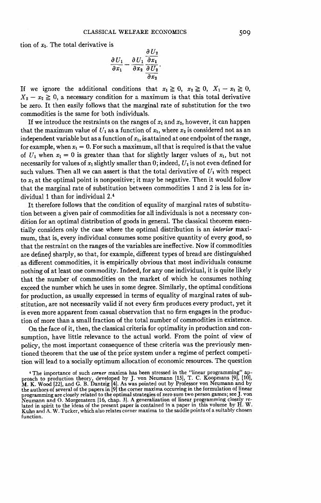
tion of xl. The total derivative is9U2

ou1 au1 dYi(x) 9X2 aU2

Ox2If we ignore the additional conditions that xl _ 0, x2 _ 0, X1-xl _ 0,X2- X2 _ 0, a necessary condition for a maximum is that this total derivativebe zero. It then easily follows that the marginal rate of substitution for the twocommodities is the same for both individuals.

If we introduce the restraints on the ranges of xi and x2, however, it can happenthat the maximum value of Ui as a function of xi, where x2 is considered not as anindependent variable but as a function of xi, is attained at one endpoint of the range,for example, when xi = 0. For such a maximum, all that is required is that the valueof U1 when xi = 0 is greater than that for slightly larger values of xi, but notnecessarily for values of xi slightly smaller than 0; indeed, Ui is not even defined forsuch values. Then all we can assert is that the total derivative of U1 with respectto xi at the optimal point is nonpositive; it may be negative. Then it would followthat the marginal rate of substitution between commodities 1 and 2 is less for in-dividual 1 than for individual 2.4

It therefore follows that the condition of equality of marginal rates of substitu-tion between a given pair of commodities for all individuals is not a necessary con-dition for an optimal distribution of goods in general. The classical theorem essen-tially considers only the case where the optimal distribution is an interior maxi-mum, that is, every individual consumes some positive quantity of every good, sothat the restraint on the ranges of the variables are ineffective. Now if commoditiesare define,d sharply, so that, for example, different types of bread are distinguishedas different commodities, it is empirically obvious that most individuals consumenothing of at least one commodity. Indeed, for any one individual, it is quite likelythat the number of commodities on the market of which he consumes nothingexceed the number which he uses in some degree. Similarly, the optimal conditionsfor production, as usually expressed in terms of equality of marginal rates of sub-stitution, are not necessarily valid if not every firm produces every product, yet itis even more apparent from casual observation that no firm engages in the produc-tion of more than a small fraction of the total number of commodities in existence.On the face of it, then, the classical criteria for optimality in production and con-

sumption, have little relevance to the actual world. From the point of view ofpolicy, the most important consequence of these criteria was the previously men-tioned theorem that the use of the price system under a regime of perfect competi-tion will lead to a socially optimum allocation of economic resources. The question

I The importance of such corner maxima has been stressed in the "linear programming" ap-proach to production theory, developed by J. von Neumann [15], T. C. Koopmans [9], [10],M. K. Wood [22], and G. B. Dantzig [4]. As was pointed out by Professor von Neumann and bythe authors of several of the papers in [91 the corner maxima occurring in the formulation of linearprogramming are closely related to the optimal strategies of zero sum two person games; see J. vonNeumann and 0. Morgenstern [16, chap. 3]. A generalization of linear programming closely re-lated in spirit to the ideas of the present paper is contained in a paper in this volume by H. W.Kuhn and A. W. Tucker, which also relates corner maxima to the saddle points of a suitably chosenfunction.

5IO SECOND BERKELEY SYMPOSIUM: ARROW

is naturally raised of the continued validity of this theorem when the classicalcriteria are rejected.

It turns out that, broadly speaking, the optimal properties of the competitiveprice system remain even when social optima are achieved at corner maxima. In asense, the role of prices in allocation is more fundamental than the equality of mar-ginal rates of substitution or transformation, to which it is usually subordinated.From a mathematical point of view, the trick is the replacement of methods of dif-ferential calculus by the use of elementary theorems in the theory of convex bodiesin the development of criteria for an optimum.5

These results have a bearing on one aspect of the recent controversy betweenProfessors Hicks and Kuznets over the concept of real national income. ProfessorKuznets [I1, pp. 3-4] argues essentially that if an individual does not consume any-thing of a certain commodity, his marginal valuation of the commodity is, in gen-eral, less than that of someone who consumes a positive quantity of that commodity.The redistributions which Professor Hicks has made use of in his treatment of realnational income are therefore imperfect. Professor Hicks, in his reply, essential-ly accepts the point [7, pp. 163-164]. But if the argument of the present paper iscorrect, it is the prices and not the marginal utilities which are in some sense pri-mary. What Professor Kuznets is getting at is the valid statement that the Hickscriterion may lead to the assertion that one situation is both better and worse thananother, for example, [18], [17, pp. 2-3]. But this possibility has no special connec-tion with the existence of corner maxima in individual utility maximization or so-cial welfare optimization.

It develops as a byproduct of the main investigation, that the use of convex setmethods also enables the criteria for optimality to cover the cases where there aregoods which are unwanted or which are positive nuisances. The assumption usuallyimplicit in past studies has been that any individual would prefer to have more ofany one commodity, holding all other commodity flows constant, to less. Providingwe consider negative and zero as well as positive prices, the theorem on the optimal-ity of the competitive price system is still valid for commodities such that addition-al quantities are useless or worse.

It should be noted, however, that there is an exceptional case in which an op-timal distribution is not achievable through the use of prices. This case seems notto have been noted previously.

In section 3, the problem of optimal economic systems is posed formally, andcertain assumptions about the functions entering therein are made. Some mathe-matical tools are presented in section 4. The necessary and sufficient conditionsfor the achievement of optimal situations are then developed in sections 5 and 6.The case where it can be assumed that unwanted goods are disposable withoutcost is discussed in section 7 and related to linear programming in its present form.Diagrammatic representations of the conclusions are presented in section 8. Anassessment of the economic meaning and probable validity of the assumptionsmade in section 3 is presented in section 9. Finally, the relevant portions of thetheory of convex sets are quickly sketched in section 10.

I A sketch of the relevant parts of the theory of convex bodies is given in the last section of thispaper.

CLASSICAL WELFARE ECONOMICS 5II

3. Formulation of the problem of optimal distribution

We suppose that we have m individuals and n commodities in the society. By acommodity bundle will be meant a vector of n components expressing the quantitysome individual will receive of each of the n commodities, the i-th componentdesignating the quantity of the i-th commodity.

ASSUMPTION 1. All quantities consumed must be nonnegative.The behavior and desires of each individual are assumed to be expressed by a

system of rules specifying for each pair of commodity bundles either a preferencefor one over the other or indifference between them. This preference pattern is as-sumed to possess the usual properties of a (weak) complete ordering6 and also suit-able continuity properties. The pattern therefore can be represented by a utilityindicator U(x) defined for all commodity bundles x in the nonnegative octant ofEuclidean space and continuous in its domain of definition, with the property thatbundle x is preferred to bundle y if and only if U(x) > U(y); see, for example,Wold [21].By a distribution is meant an assignment of the n commodities among the m in-

dividuals. A distribution X is thus an array of mn numbers Xi,, designating theamount of commodity i to be given to individual j. For fixed j, the numbersXlj, . . . , Xq, form the commodity bundle to be given to individual j; for agiven X, this bundle will be designated by Xj. Implicit in the above notation forutility is the following important assumptiofi:

ASSUMPTION 2. The desirability of a distribution X to individual j is solely dic-tated by the desirability to him of the commodity bundle Xi.

This is the assumption that individuals act selfishly. Hence, for any given dis-tribution X, the desirabilities to individuals 1, . , m are represented by the num-bers U1(X1), . ., Um(Xrn), respectively.

If x and y are commodity bundles and t a real number between 0 and 1, we shallunderstand by the notation tx + (1- t)y the commodity bundle whose i-th com-ponent is txi + (1 - t)yi. If x and y are indifferent in the judgment of an indi-vidual, then it is usually assumed in economic theory that the convex combinationtx + (1 - t)y is preferred to either x or y if t is different from 0 to 1.

AsSUMPTIoN 3. For allj, if Uj(x) = Uj(y), and 0 < t < 1, then Uj[tx+ (1- t)y]> Uj(x).

Naturally, the possibilities for a social choice among alternative distributionsare limited by the limitations on production. Such limitations can be phrased by

saying that the social commodity bundle S Xi must lie in a set T, where by thej=l

m

notation z Xi is meant a bundle whose i-th component is the sum of the i-th com-j=l

ponents of the bundles X1, . . . , Xm. The set T will be known as the transforma-tion set.

6 That is, (1) for any two commodity bundles A and B, either A is preferred to B or B to A orthe two are indifferent; (2) if A is preferred or indifferent to B and B is preferred or indifferent toC, then A is preferred or indifferent to C (transitivity).

5I2 SECOND BERKELEY SYMPOSIUM: ARROW

ASSUMPTION 4. The transformation set T is nonnull, convex and compact;7 further,if x is a bundle in T, xi > Ofor every component of x.

DEFINITION. A distribution X* is said to be optimal in T if (a) E X belongsj=l

to T; and (b) if there is no other distribution X such that E Xj belongs to T and

Uj(X,) _ Uj(X,) for all j, with the strict inequality holding for at least one j.It is clear that for any distribution which is nonoptimal, there is another dis-

tribution in which everybody is at least as well off and at least one person betteroff. The optimal distribution of a fixed stock of goods is the special case where Tconsists of a single point.

4. Some preliminary lemmasAn elementary mathematical consequence of the assumptions and other state-

ments from the elementary theory of convex sets will be presented here for lateruse.LEMMA 1. For givenj and given number U, the set of vectors xfor which Uj(x) > U

is closed and convex; further, if x and y belong to the set and 0 < t < 1, then Uj[tx +(1 - t)y] > U.

PROOF. Let x and y both belong to the indicated set. Without loss of generality,we may suppose(1) U < Us(x) < Uj(y).Define f(t) = Uj[tx + (1 - t)y]; this is a continuous function on the closed inter-val (0, 1) and so has a minimum there at some point to. Suppose 0 < to < 1; thenwe can obviously choose t1, t2 so that 0 < ti < to < t2 < 1, f(t1) = f(t2) >_ f(to).But from the definition of f(t) and assumption 3, f(to) > f(t1) under these circum-stances. Hence, it must be that to = 0 or to = 1; since f(O) _ f(1) by (1), f(t) >f(1) > U for all t such that 0 < t < 1, so that the set is convex.

That this set is closed follows immediately from the continuity of the func-tion Uj(x).

LEMMA 2. Let A be any closed convex set and x* a boundary point of A. Then

there is a vector (pi,..., pn), pi id O for some i, such that for all x in A, z pixi _i=l1

n

Spix*l.i=lLEmmA 3. Let A and B be closed convex sets such that A has at least two points

and no internal point of A is also a point of B. Then there is a vector p = (Pi, ., P.),not all of whose components are zero, and a number c such that,

n

E~pixi _ c for all x in A

n

EPixi <_ c for all x in B .

i=l

7 A set is said to be nonnull if it contains at least one element. It is said to be convex if for anytvo bundles x and y in the set and any t such that 0 < t < 1, the bundle tx + (1 - £)y also be-longs to the set. Finally, a compact set is a bounded set such that no sequence of points in theset converges to a point outside the set.

CLASSICAL WELFARE ECONOMICS 5I3

These lemmas and the definitions of internal and external points are discussed insection 10 below.

5. The case of a single individualIf m = 1, the distribution X reduces to a single vector or commodity bundle x.

Then x* is optimal in T if U(x*) _ U(x) for all x in T, that is, if x* maximizesU(x) for x in T. [Here, the subscript 1 on Ul(x) has been omitted.] This case isof some interest because in certain respects the general case can be reduced to it.THEOREM 1. There is a unique optimal point x* in any T.PROOF. Since U(x) is continuous and T is nonnull and compact, there is at

least one maximum of U(x) and therefore at least one optimal point. Supposex* and y* are both optimal; then U(x*) _ U(y*), U(y*) _ U(x*) and thereforeU(x*) = U(y*). Let z* = 2x* + iy*. Since T is convex and x* and y* both be-long to T, z* belongs to T. By assumption 3, U(z*) > U(x*), contrary to theassumption that x* and y* are both optimal. Hence, the optimal point is unique.

DEFINITION. The bundle x* is said to be a point of bliss if U(x*) _ U(x) forall x.

Clearly, if the point of bliss belongs to the transformation set T, it is optimal.Usually, an optimal point is not a point of bliss; that is, the optimal point for agiven set of production restraints is not the best point the individual would wishfor were he unrestrained.LEMmA 4. If x* is optimal in T but not a point of bliss, then there is a vector p such

that (a) z pixi _ E pi4 for all x such that U(x) _ U(x*); (b) S pixi _

E pix for all x in T; pi # Ofor at least one i.

PROOF. Let V be the set of vectors x such that U(x) _ U(x*). From theorem 1and the definition of an optimal point, V and T have only the point x* in common.Suppose x* were an internal point of V. Then, by definition, in some linear sub-space of the commodity n-space, x* would be surrounded by a neighborhood ofpoints all in V, and therefore there would exist two points x and y in V such thatx* = tx + (1 - t)y, where.0 < t < 1. By lemma 1, U(x*) > U(x*), a contradic-tion. Therefore, x* is an external point of V, and hence no internal point of V be-longs to T. Since x* is not a point of bliss, V contains at least one point besides x*.By lemma 1 and assumption 4, V and T are closed convex sets. Lemma 4 then fol-

lows from lemma 3, since x* belongs to both V and T, so that S pix* = c.n n i=l

LEMMA 5. For a given x*, let p be such that S pixi > E pixVfor all xfor whichi=l1=

U(x) _ U(x*) and such that pkx*k $ Ofor some k. Then x* uniquely maximizes U(x)n n

subject to the condition that S p1x1 _ E ptxl.PROOF. Suppose the conclusion is false. Then, for some x # x*,

n n

(1) Pix*,i=l i=l


(2) U(x) _ U(x*).n a

From the hypothesis, (2) implies that pixi _ pix, so that, from (1),n n 1

2 2~~~=1 t=

E pixi = E pix. Let y = 2x + 2x*. Then,ili=l1

n n

(3) PiYi Pix*i.

By hypothesis, xk > 0; therefore, yk > 0. Define the vector z, as follows: zi = yifor i $ k, Zk = yk + e. For all e sufficiently close to 0, zi 2 0 for all i. From (2)and lemma 1, U(y) > U(x*); therefore, for all e sufficiently close to 0,

(4) U (z) > U (x*) .

By hypothesis, pk #! 0. Choose f sufficiently close to 0 to satisfy (4) and of a signopposite to Pk. Then, by (3)

n n n

( 5) P i Zi = EPiyi + ePk <Pix*t-

i=l i=l i=l

But the existence of a vector z with properties (4) and (5) contradicts the hy-potheses of the lemma.

DEFINITION. The "price" vector p is said to equate supply and demand at x* if (a)n n

x* uniquely maximizes U(x) subject to the condition S pixi _5 pix4, (b) x*i-i i-i

n

maximizes , pixi subyect to the condition that x belongs to T.

If we interpret the vector p as a set of prices, one for each commodity, then clear-ly (a) states that x* constitutes the quantities demanded of each commodity at thegiven price levels, provided sufficient income is supplied to purchase x* but no more,under conditions of perfect competition, while (b) states that x* will also be thequantities supplied under the assumption of profit maximization under competi-tive conditions. It is not implied that the price vectQr is unique, nor, of course,need there exist a price vector with the above properties for every x in T. Indeed,such price vectors will only exist for optimal points, as we shall see.

THEOREm 2. If there is a vector p which equates supply and demand at x*, then x*is an optimal point.

PROOF. Suppose x* is not optimal. Then for some y in T, U(y) > U(x*). Since

x* uniquely maximizes U(x) subject to the conditions E pixi < pix, iti=l i-1

must be that piyi > E pix!. But this contradicts the hypothesis that x*

maximizes the linear function z pixi for x in T.i=1

Theorem 2 states that if a set of prices can be found which equate supply anddemand, then the resulting situation is optimal. The triviality of the reasoning

CLASSICAL WELFARE ECONOMICS 5I5

leading to this sufficient condition for optimality is in contrast with the more com-plicated proof leading to the converse theorem, which in fact is not valid in com-plete generality. The precise statement follows.THEOREM 3. For any optimal point x*, there is a vector p with at least one nonzero

n n

component with the following properties: (a) , pixi _ ^ pix* for all x such thati-1 i=l

U(x) _ U(x*); (b) there is a commodity bundle y*, where y* > x* for all i, which

maximizes the profit function , pixi subject to the condition that x be in T; (c) if x*

is not a point of bliss, then y = x* for all i in (b); (d) if either pkxk* 0 for some kor x* is a point of bliss, then x* uniquely maximizes U(x) subject to the condition thatn n

i pixi piX*.i -i t=1

PROOF. If x* is not a point of bliss, then statements (a-c) are made in lemma 4.Suppose x* is a point of bliss which is optimal in T. Let T be the least upper boundof values of t for which tx* belongs to T. Since T is a closed set, Trx* belongs to T;also, clearly, r > 1. Let y* = TX*. Since x* > 0 for each i, by assumption 4,y* _ x* for each i. For t > T, tx* does not belong to T. Therefore every neighbor-hood of y* contains points not in T, so that y* is a boundary point of T. By lemma

2, there is a price vector p such that S pixi < S pay for all x in T, establish-i-1 i-1

ing (b). Now suppose for some x - x*i, U(x) _ U(x*).' Then if y = 2x + -x*,U(y) > U(x*) by lemma 1, which contradicts the assumption that x* is a pointof bliss. Therefore, the set of points for which U(x) > U(x*) contains just thepoint of bliss x*, so that (a) is trivial. Part (c) is irrelevant if x* is a point of bliss.Finally, the previous argument shows that U(x*) > U(x) for all x X x*, so that(d) follows trivially in case x* is a point of bliss.

If x* is not a point of bliss, then (d) follows from (a) by lemma 5.Parts (a-c), particularly, characterize optimal points. For a point of bliss, it is

possible to set prices so that at least as much will be produced, under the assump-tion of profit maximization, of each commodity as is used at the point of bliss.Then, if enough income is given the consumer so that he can purchase the quan-tities at the point of bliss evaluated at the prices just set, he will in fact purchasethem. The more interesting case is that in which the point of bliss, if any, is notcontained within the available production possibilities. Then prices can be set sothat simultaneously the optimal point will maximize profits to producers andminimize the cost of achieving the associated (optimal) utility level to consumers.Apart from an exceptional case, that is, when the optimal bundle contains positivequantities only of those goods with zero price, it is also true this minimum cost

property is equivalent to the proposition that the individual maximizing hisutility subject to the constraint that his expenditures at given prices not exceed a

quantity sufficient to purchase the optimal bundle, will in fact choose that bundle.Theorem 3 says, in effect, that an optimal point can be achieved by suitable

choice of prices under a competitive system. By itself, this hardly distinguishes


the price system from others. For example, obviously any point in T, and in par-ticular the optimal point, can be achieved by rationing. Theorem 2 adds, however,the important quality that once a bundle has been chosen by means of the pricesystem, we know that it is optimal, a quality not shared in as direct a way, atleast, by direct controls. Of course, the validity of these theorems is dependentupon the validity of assumptions 1-4.

It is to be noted that no assumptions or conclusions as to the signs of the priceswere made or drawn. At this stage, the presence of unwanted commodities in con-sumption or of goods whose production is made easier rather than harder by theemployment of resources to produce other goods is not excluded.

6. The case of many individualsWe will now return to the general case, where m, the number of individuals may

be more than 1.DEFINITION. For a given optimal distribution X* and a given individual k, let Tk

be the set of all vectors xfor which there exists a distribution X such that (a) x = Xk;(b) Uj(X3) _ Uj(X*) for all j #D k; (c) z Xj belongs to T.

j='

If we start from a given optimal distribution X*, then Tk is the set of all possiblebundles which individual k can secure for himself if he is given complete charge ofthe distribution of goods subject only to the conditions that the distribution becompatible with the production possibilities and at the same time not bring anyother individual to a position in which the latter is worse off than he would beunder the given optimal distribution. In order that X* be in fact optimal, it is clearthat individual k must find that the best vector x in Tk with respect to his utilityfunction be xk*, for otherwise there would be another distribution compatible withthe production possibilities in which no individual other than k is worse off thanhe would be at X*, while individual k would have a way of being better off. Foran optimal distribution, then, Xk* must maximize Uk(X) subject to the conditionthat x belongs to Tk; this must hold for each k. The set Tk then plays, in effect, therole of the production possibilities open to individual k, and the results of the pre-vious one individual case can be used here. Incidentally, there is one difference be-tween the sets Tk and the set T; the former, but not the latter, may (and usuallywill) include bundles with negative components. Their inclusion in Tk is in factessential to the proof following. However, their exclusion from T was not in factmade use of in the proofs of section 5, so that the theorems there proved are stillapplicable where relevant.LEmA 6. The sets Tk are nonnull, closed and convex.PROOF. By definition, the bundle Xk* belongs to Tk, so that it is nonnull.Let xn be a sequence of points in Tk which converge to a given point or bundle x.

For each xn, then, by definition of Tk, there is a distribution Xn such that

(1) E X'n belongs to T,j=f

(2) U3 (Xcn) > Uj (Xj*) for allj F' k


(3) xn = Xkn for each n .

Since by assumption 1, Xn;1 > 0 for each n, i, and j #d k, it follows thatm

(4) 0 _ Xn_ E Xni, -xni forj FD k.i=l

Since T is a bounded set by assumption 4 and x'n a bounded sequence, it followsfrom (4) and (2) that the sequence Xi, is bounded for each fixed i andj $ k. Thenwe can choose a subsequence of the integers, n1, . ., n, . ., such that each ofthe sequences X7;. converge; by (3), the sequences X" also converge. Let Xij =lim Xc;. From (3), it follows that, for each i,7 .-4co

(5) Xik = xi, or X= Xk.

From (2) and the continuity of Uj(x),(6) Uj (X,) > Uj (X*) for all j F# k .

From (1), L X7" belongs to T for each r. Since T is a closed set, it follows thatj=l

in the limit,m

(7) Xi belongs to T.j=l

From (5-7), x belongs to Tk, so that Tk is closed.Now let x and y be any two elements of Tk. Then, there exist distributions

X and Y such that,

(8) X = Xk, Y = Yk

(9) Uj (X,) _ Uj (X*) , Uj (Yj) _ Uj (X*) for all j F- k,mn m

(10) Xi andE Yi both belong to T.

Let z = tx + (1 - t)y. Define the distribution Z so that Zj = tX, + (1 -t) Y,.Then, by (8),

(1 1) Z = Zk -

Assume 0 _ t < 1. By lemma 1, the set of all bundles for which Uj(x) _ U,(X*)is convex. From (9).

(12) Uj (Z,) _ U (X>) for allj F$ k .

Finally, since T is convex by assumption 4, it follows from (10) that

(13) E Zj belongs to T.F=s

From (11-13), z belong to Tk, So that Tk iS convex.

5i8 SECOND BERKELEY SYMPOSIUM: ARROW

Lemma 6 formally establishes that Tk has all the relevant properties of T.LEMMA 7. If X* is optimal in T, then X} is optimal in T,for eachj.PROOF. Suppose not. Then there is some individual k and some bundle x in Tk

such that Uk(x) > Uk(Xk), and hence a distribution X such that,

(1) Uk (Xk) > Uk (Xk) ,

(2) Uj (X,) _ Uj (Xi*) for all j $ k,

(3) E Xj belongs to T.3=1

(1-3) contradict the statement that X* is optimal in T.Lemma 7 formally reduces the optimality problem for the society to that for

single individuals. Without further argument, it could be deduced that there is aset of prices for each individual such that utility maximization under a budget con-straint would lead him to choose the given optimal point [subject to the minor ex-ception noted in theorem 3(d)]. However, a stronger statement can be made; thesame set of prices will do for all individuals.

THEOREM 4. If X* is optimal in T, there is a vector p, for which pi # Ofor some i,

with the following properties: (a) for each j, E pixi, p,X., for all x such thatm

Uj(x) _ Uj(X*); (b) there is a vector y* such that XX*J < y* for all commodities ijl1

n n

and j pixi poylfor all x in T; (c) if, for some j, X, is not a point of bliss,i-1 i-1

mthen y* = Xi* in (b); (d) for any individual j for whom either pkXk*j O for

j=l

some k or Xj* is a point of bliss, X, uniquely maximizes Uj(x) subject to the budgetn n

condition E pPxi < X.i-1 i-1

PROOF. Let V, be the set of all bundles x for which Uj(x) _ Uj(X). We willconsider two cases in proving the theorem.

Case 1. For somej, X, is not a point of bliss. Let k be the value of j in ques-tion. By lemma 7, Xk is optimal in Tk. By lemma 4,

n nt

(1) 3 pixi _ PiX*k for all x in Tk,i=l i=l

(2) piXXk for all x in Vk.i-1 i1=

Choose an individual q distinct from k. Let x belong to Vq, which is nonnull sinceit contains X*. Then Uq(x) _ Uq(X*). Define the distribution X as follows:Xk = Xk* + Xq*-X, Xq = XI Xi = X; for i distinct from both q and k. Then, itis easy to see that Xk belongs to Tk; by (1),

n n

EPi (X*ik+ XTq xi) <_ E Piik,

CLASSICAL WELFARE ECONOMICS 5I9or

n n(3) Pixi >- EpiXT,

i=l i=l

(3) holds for any x in Vq, where q is any individual distinct from k.. From (2), then,n n

(4) Pixi >- PiX*j for all i and all x in Vi,il i=l

which is (a).Now let x be any element of T. Define the distribution Y as follows: Yj =X

for allj # k, Yk = X- Xj*. Clearly Yk belongs to Tk. By (1),j^dk

n n

Pi (Xi- xij) _ E Pi (Xik),i=l ~~jOk i=l

orn n n

(5) iXi Pi (X*j) for all x in T,

which establishes (b) and (c). Finally, (d) follows from (a) by lemma 5.Case 2. X>* is a point of bliss for allj. Let T be the least upper bound of the values

of t such that t ( X) belongs to T, y* r( X). Then T _ 1. As in theo-

rem 3, y* is a boundary point of T, so that, by lemma 2, we can choose p so thatn n

(6) E Ppiy* for all x in T.i=l i-I

Clearly,

(7) X*j y* for all i,i=l1

so that (b) is valid. As shown in the proof of theorem 3, (a) and (d) are trivial inthis case.

DEFiNITION. The vector p is said to equate supply and demandfor the distribution

X* if (a) for each j, X, uniquely maximizes Uj(x) under the constraint z pixi <i=l

E piX*j; (b) for all x in T, Pixi P (P X )i=l i=l i=l j=1

THEOREm 5. If there is a vector p which equates supply and demand for X*, thenX* is optimal.

PROOF. Suppose not. Then there is a distribution X such that(1) Uk (Xk) > Uk (Xk) for some k,

(2) Uj(X) Uj (Xj*) for allj $k

(3) Xi belongs to T.j=l


From (1) and condition (a) of the preceding definition, it follows thatn n

(4) PiXik > PiX*ik.n n

From (2) and condition (a), for each j F4 k, either piXij > 5 piX*j, ori=l i=l

Xj = X,, so that,n n

(5) EpX _ piX*ij for all j 7-' k.i=l ~~~i=l1

From (4) and (5),n mn m

(6) * S Pi ( Xij) ~> Pi ( X*j)(6)Pi)_ i

But (3) and condition (b) imply that (6) is false. Hence, the theorem is true.Theorems 4 and 5 together define the role of the price system in the same way

as for a single individual in section 5. Disregarding the existence of points of bliss(for all too good empirical reasons) leaves only the case where piXi* = 0 for all ifor some individual j as an exceptional case of an optimal point unreachable bythe price system. In this case, the optimal situation requires that individualj con-sume only free goods. The individuals for whom the conclusion of theorem 4(d) isvalid have the right to consume as much of the free goods as they wish in maximiz-ing their utility under the budget constraint. Hence, it must be that at the bundlesto which they are entitled under the optimal situation they are saturated with re-spect to the free goods; either an increase or a decrease in the quantity of any ofthe free goods, holding the quantities of other goods constant, would decreasesatisfaction. The reason that the price system fails is that the prices of the goodsconsumed by individualj must be zero to permit other individuals to become satu-rated with those goods, but at the same time there is no restraint compelling in-dividual j to stick to the quantity of free goods allotted to him under the optimalconditions, since, of course, he could, under the price system, consume as much ofthese as he pleases. Only by coincidence would he also be saturated with thosefree goods at a zero level of other goods.

7. The case of free disposalIt is common in discussions of production to make implicitly or explicitly the

followingASSUMPTION 5. If x belongs to T and y is a vector such that 0 _ yi _ xifor every

commodity y, then y belongs to T.The argument generally runs that, if necessary, one could always produce y by

producing x and then discarding the quantities xi- yi of the commodities i. Thisamounts to assuming that there is a method of disposal of surplus products whichis costless to producers. Under these conditions, it turns out that we can confineourselves to nonnegative prices.

For the following lemma, let us define, for a given integer q _ n, the projectionof an n-vector x to be the q-vector whose components are xi, . . . , x,. The projec-

CLASSICAL WELFARE ECONOMICS 52I

lion of a set T will be the set of all points in q-dimensional space which are projec-tions of points of the set T.

LEMMtA 8. Let x* belong to the transformation set T, and suppose x* > Ofor i = 1,... , q, x* = Ofor i = q + 1, ... , n. Let x` and T' be the projections of x* and T,respectively. Then, if x*'is a boundary point of T' in q-dimensional space and if as-

sumption 5 holds, there is a vector p such that x* maximizes pixi for x in T, andi=l

such that pi > Ofor all i, pi > Ofor some i.PROOF. Clearly, T' is closed, convex, and nonnull. By lemma 2, there exists a

vector (pi, . .. , p,) such that

q q

( 1 ) E ~~pixi= pix4 for all x in T', pi .- 0 for some i,ili=l1

since x*' is a boundary point of T'. For a given r such that 1 < r < q, define then-vector y in T so that yi = x* for i F$ r, yr = 0. By assumption 5, y belongs to T.Let y' be the projection of y; by (1), it follows that p.x* _ 0. By construction4> 0, so that Pr _ 0. This holds for all r between 1 and q, inclusive. From (1),then, pi > O for at least one value of i. Define p =0for i = q + 1, . . ., n. If

n q

x belongs to T and x' is the projection of x, then E pixi = E pixi. The lemmai=l i=l

then follows from (1).LEMMA 9. Let X* be an optimal distribution in which, for some individual k, Xk

is not a point of bliss. If p satisfies the conclusions of theorem 4 and if assumption 5holds, then pi > 0 for at least one value of i.

nPROOF. Suppose pi _ 0 for all i. Then E piX*s < 0 for all j, and

i=ln n

pPi ( XXj) < 0 . But by assumption 5, the point (O,.. , 0) belongs to T;

m ~ ~ ~ ~~nn in

since the point pX maximizes pixi for x in T, p (E X*j) _) , and

n m ntherefore pi ( Xj) = 0, so that for each j, E piX*,= 0. Since p satisfies

il j=l i=l

theorem 4(a),n

(1) EPixi_OforallxinVk.

By hypothesis, there is a vector y for which

(2) Uk (y) > Uk (Xk)-

Since pi -$ 0 for some i, there is an r such that pr < 0. Let z be any vector forwhich zr > 0; let w = ty + (1 - t)z. For all t < 1, wr > 0; but for t sufficientlyclose to 1, it follows by continuity from (2) that Uk(w) > Uk(Xk), so that


n n

S pw1i > 0 by (1). But since pi _ 0 for all i, Pr < 0, i piw1 < 0, a contra-i-I i=l

diction.THEOREm 6. If X* is an optimal distribution and if assumption 5 is valid, then

there is a set of prices p satisfying the conclusions of theorem 4 for which pi _ O forall i, pi > Ofor at least one i.

PROOF. First suppose that Xi* is a point of bliss for all j. Let y* be the point inT which enters into theorem 4(b). By renumbering the commodities, it may besupposed that y* > 0 for i = 1,.... q, y* = 0 for i = q + 1,... ,n. Let y*'and T' be the projections of y* and T respectively. Suppose that for some t > 1,the point ty*' belongs to T'. Then there is a point z in T such that zi = ty* for i = 1,* , q, zi _ 0 for i = q + 1, . .. , n. By construction, the point ty* has the samefirst q coordinates as z, while the last n - q are zero, so that ty* belongs to T byassumption 5 contrary to the construction of y*. Hence, for all t > 1, ty*' does notbelong to T', and y*' is a boundary point of T'. Conclusion (b) of theorem 4 thenfollows from lemma 8. Conclusions (a) and (d) follow trivially in this case, asbefore.Now suppose that for some j, Xi* is not a point of bliss for individual j. By lem-

ma 9, there is a vector p' satisfying the conclusions of theorem 4 with pi > 0 forat least one value of i. It will be shown that any negative price in this vector canbe replaced by a zero price without changing the conclusions of this theorem.Suppose pr/ < 0. Define p so that pi = P' for i F# r, pr = 0; it will be shown that phas the same properties as p'. By theorem 4(b) and (c),

(1) Pi - ( X*j) for all x in T.ili=l1j=l

In (1), first let x be such that xi = E X*' for i 5 r, X, = 0. By assumption 5,j=l

x belongs to T. Then p' ( X*jr)O; sincepr <r0 E = 0,so that

(2) X*j=O for all j,

i=1 j=1 i=1 j=l

Now, for any x in T, define y so that yi = xi for i $ r, yr = 0. By assumption 5,y belongs to T; by (1),

n n m(4) E Piyi _< E Pi X*S)

il i=1 j=l

n n

But E PiYi = E pixi; from (3) and (4),i=l i=l


n n m(5) pixi pi( X*j) for all x in T,

i-1 i-1 j=1

which is conclusion (c).By theorem 4(a),

n n

(6) Pp.xi _ j ptX*J for all j and all x in Vj.i-i s-1

From (2),n n

(7)~~~~~~~P tx 1j P i xX*j .

i-1 i=l

nn

Since xr _ 0 and p' < pr, j Pixi _ E pix4. From (6) and (7), then,i=l1 i=l

n n

Spixi _ z piX* for all j and all x such that Uj(x) _ Uj(Xj*), which is con-

clusion (a). As in the proof of theorem 4, part (d) follows from (a) by lemma 5.If the new vector p still has negative components, they may be removed by the

above process. Since p' had at least one positive component, which is undisturbedby subsequent operations, each of the successive price vectors has at least one non-zero component.

DEFINITION. A bundle x* of goods in the transformation set T will be said to beefficient iffor some set of utility functions Uj(x) (j = 1, . . ., m), there is a distribu-

tion X* such that (a) X* is optimal in T; (b) X = x*; and (c) for some j, Xi* is

not a point of bliss for individualj.This definition of efficient points is not precisely equivalent to that used in

linear programming by T. C. Koopmans and others [4], [9], [10], [22] but conveysthe same general meaning. The efficient points of T are just those which could beused in some optimal distribution. Clause (c) is inserted to exclude trivialities.Without it, by suitable choice of the functions Us(x), every point of T would beefficient. Of course, when every individual is at his point of maximum absolutesatisfaction, the concept of economic efficiency becomes meaningless.

THoEoREm 7. Under assumption 5, thefollowing are each a necessary and sufficientn n

condition for x* to be efficient: (a) E pixi _ , pix for all x in T and for some p

for which pi _ Ofor all i, pi > Ofor some i; (b) there is no y in T for which xi < yifor all i.

PROOF. First, it will be shown that (a) is a necessary and sufficient conditionfor x* to be optimal. The necessity has already been shown in theorem 6. For thesufficiency, let X* be a distribution which gives x*/m to each individual. For each

n

individual j, let Uj(x) =- (xi- x*/m - pi)2, defined only for those valuesi-1

of x for which xi 2 0 for all i. This utility function has an absolute maximum atthe point x*/m + p, and its indifference surfaces are concentric spheres about


that point. From the geometric picture, or algebraically with the aid of Schwarz'sinequality, it is easy to see that assumption 3 is verified. By simple algebraicmanipulation, it can be seen that x*/m uniquely maximizes Uj(x) subject to the

condition z pixi < pi(xe/m). From the statement of condition (a), and

theorem 5, it follows that X* is an optimal distribution for the given set of utilityfunctions and therefore that x* is an efficient point.To show that (b) is also a necessary and sufficient condition for x* to be an

efficient point, it will be shown that (b) is equivalent to (a). If there were a y in Tn

such that yi > x* for all i, then, if pi _ 0 for all i, pi > 0 for some i, pixt <i=l1n

S piyi, contrary to (a). Hence, (a) implies (b).i=l1

For the converse, renumber the commodities so that x* > 0 for i = 1, . . . q,x*= 0fori= q+ 1, ...,n.

Case 1. For some y in T, x* < yi for i = 1, . .. , q. Suppose that for eachi=q + 1, . . ., n, there is a vector x(i) in T such that xii) > 0. Let z=n n

S tix(i) + toy, where ti = 0 (i = 0, ... , n), E ti = 1. Since T is convex, z be-i=0+1 i=O0longs to T. For ti sufficiently small (i $d 0), x* < zi for all i, contrary to (b). Hence,for some r between q + I and n,xr = Ofor all x in T. Let p, = 1, pi = O for i # r;

n

then E pixi = 0 for all x in T, and (a) holds trivially.

Case 2. There is no y in T such that x* < yi for all i _ q. Let x*' and T' be theprojections of x* and T, respectively. Let z be a q-vector with zi = x* + e; thenfor all positive e, z does not belong to T'. Hence, x*' is a boundary point of T', and(a) holds by lemma 8.

Assumption 5 relates to free disposal on the part of the producers. It might in-stead be presupposed that it is the consumers who can dispose without cost ofotherwise unwanted goods.

ASSUMPTION 6. For each j, if xi _ yi for all i, Uj(x) _ Uj(y).For convenience, let x < y mean that xi _ yi for all i, xi < y, for some i. Be-

cause of assumption 3, it easily follows that increasing the stock of one commodity,holding all others fixed, actually increases the desirability of a bundle. Hence, as-sumption 6 really implies insatiability of wants.LEMMA 10. If x < y, then under assumption 6, Uj(x) < Uj(y).PROOF. By assumption 6, Uj(x) . Uj(y). Suppose Uj(x) = Uj(y). Let z=

2x + 2y; by assumption 3, Uj(z) > Uj(y), which is impossible since zi _ yi for all i.If assumption 6 holds, we will understand in the definition of an efficient point

that the utility functions referred to must satisfy that assumption.THEOREM 8. Under assumption 6, a necessary and sufficient condition that x* be

n n

an efficient point is that for some p such that pi > Ofor all i, E pix _ E pix*forall xin.i=l

all x in T.r


PROOF. Suppose x* an efficient point. Then there is an optimal distribution X*and a price vector p satisfying the conclusions of theorem 4. By lemma 10, X* isnot a point of bliss for any j. For any j,

n n

(1) pixi_ S piX*ijforall x in V3.

For any r = 1, ., n, let yi = X7- for i F6 r, yr> X,*. By assumption 6, y be-longs to Vj. By (1), pr(yr- X*j) _ 0, so that Pr>0_ or

(2) Pi _ O for all i.

By theorem 4, p, F 0 for some s; by (2), p8 > 0. For any r $D s, let zi = y1 fors5, zs = YJ- e. By lemma 10, Uj(y) > Uj(X7); by continuity, Uj(z) >

U1(X7) for e sufficiently small but positive. By (1), Pr(yr- X*) p.E > 0, orpi > 0 for all i. Since p also has properties (b) and (c) of theorem 4, the conclusionfollows from the assumption that x* is an efficient point.

Conversely, for each individual j, let Uj(x) = ai log (xi + 1/n), definedi=l

only for those values of x for which xi _ 0 for all i. If we define f(t) as in the proofof lemma 1, it is easy to verify thatf"(t) < 0 for all t if ai > 0 for all i. Hence, theminimum attained by f(t) over the closed interval (0, 1) must be attained at anendpoint; iff(O) = f(1), thenf(t) > f(O) for 0 < I < 1, so that assumption 3 is ful-

n

filled. Choose ai = pi(x* + 1)/ E pixA. Since Uj(x) increases with each variable

xi, its maximum under a budget constraint will occur on the boundary of the con-straint. The maximum can therefore be obtained by using Lagrangian multipliers

n n

with the constraint E pixi = S pi(x*i/m), and the maximum turns out to bei=l i=l

attained uniquely at x*/m.THEOREM 9. If assumption 6 holds, then a necessary and sufficient condition that

X* be an optimal distribution is that there exists a set of prices p, with pi > Ofor all i,m ~~~~~n

such that S X* maximizes E pixi for x in T and such that X* maximizes Uj(x)

iin m

for all x such that E pYxi pix*.i=1 j=I

PROOF. This theorem follows easily from theorems 4, 5, and 8; since pi > 0 forall i, the exceptional case in theorem 4(d) does not arise unless X3* = 0 for all i;but in that case the theorem is trivially valid.

This theorem is, of course, the classical theorem of the applicability of the pricesystem under insatiable wants extended to include corner maxima.

In connection with free disposal, it may be remarked that the use of the pricesystem to achieve a distribution where all individuals are at a point of bliss, as intheorem 4(b), implied a mechanism of free disposal somewhere in the system, sinceproducers' profit maximization will, in general, lead to an excessive supply.


8. Some diagrammatic representationsIn the case of two individuals, two commodities, and a set T containing just one

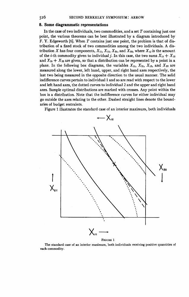
point, the various theorems can be best illustrated by a diagram introduced byF. Y. Edgeworth [6]. When T contains just one point, the problem is that of dis-tribution of a fixed stock of two commodities among the two individuals. A dis-tribution X has four components, XIn, X12, X21, and X22, where Xii is the amountof the i-th commodity given to individual j. In this case, the two sums Xi, + X12and X21 + X22 are given, so that a distribution can be represented by a point in aplane. In the following box diagrams, the variables Xll, X21, X12, and X22 aremeasured along the lower, left hand, upper, and right hand axes respectively, thelast two being measured in the opposite direction to the usual manner. The solidindifference curves pertain to individual 1 and so are read with respect to the lowerand left hand axes, the dotted curves to individual 2 and the upper and right handaxes. Sample optimal distributions are marked with crosses. Any point within thebox is a distribution. Note that the indifference curves for either individual maygo outside the axes relating to the other. Dashed straight lines denote the bound-aries of budget restraints.

Figure 1 illustrates the standard case of an interior maximum, both individuals

*X2

XII~~~~~~2

FIGURE 1

The standard case of an interior maximum, both individuals receiving positive quantities ofeach commodity.


receiving positive quantities of each commodity. By setting prices positive and pro-portional to the direction numbers of the normal to the line separating the in-difference curves at their point of tangency, the indicated optimal distribution canbe obtained by the workings of the price system.

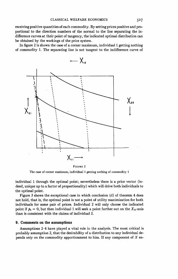
In figure 2 is shown the case of a corner maximum, individual 1 getting nothingof commodity 1. The separating line is not tangent to the indifference curve of

1.1 ~~ ~ ~ ~ 1

X22

Xii~~~~~I

FIGuRE 2

The case of corner maximum, individual 1 getting nothing of commodity 1

individual 1 through the optimal point; nevertheless there is a price vector (in-deed, unique up to a factor of proportionality) which will drive both individuals tothe optimal point.

Figure 3 shows the exceptional case in which conclusion (d) of theorem 4 doesnot hold, that is, the optimal point is not a point of utility maximization for bothindividuals for some pair of prices. Individual 2 will only choose the indicatedpoint if pi = 0, but then individual 1 will seek a point further out on the Xi,-axisthan is consistent with the claims of individual 2.

9. Comments on the assumptionsAssumptions 2-4 have played a vital role in the analysis. The most critical is

probably assumption 2, that the desirability of a distribution to any individual de-pends only on the commodity apportionment to him. If any component of X en-


tered as a variable into the utility functions of more than one individual, the wholeanalysis will be vitiated as it stands. Conspicuous consumption of the type en-visioned by Veblen is a case where there is a negative interrelation between the con-sumption of one individual and the welfare of another. The drive for income

/EX 12

I Z ^ v X- X22

X I

FIGURE 3

The exceptional case in which conclusion (d) of theorem 4 does not hold

equality and similar concepts of social equity, to the extent that it is shared by in-dividuals who stand to lose from a purely individualistic viewpoint, representsanother case of this type.

The empirical importance of this phenomenon has been stressed by Veblen [20]and more recently by Professor J. S. Duesenberry [5]; references to other studies areto be found in a paper by Dr. H. Leibenstein [13, especially pp. 184-186]. Some ofthe formal implications for the problem of optimal allocation are discussed byProfessors Pigou, Meade, Reder (see the references in Leibenstein), Tintner [19],and Duesenberry [5, pp. 92-104]. The general feeling is that in these cases, optimal


allocation can be achieved by a price system, accompanied by a suitable systemof taxes and bounties. However, the problem has only been discussed in simplecases; and no system has been shown to have, in the general case, the importantproperty possessed by the price system and expressed in theorem 5; not only canoptimal distributions (usually) be achieved by the price system but any distribu-tion so achieved is optimal.

I have argued elsewhere [1], [2] that if we seek distributions which are not merelyoptimal in the above sense but uniquely best in some social sense, then it must beassumed that the utility functions are interdependent, to the extent, at least, thateach individual has standards of social equity. These imply that preferences asamong distributions depend not only on the consumption of the individual butalso among the distribution of welfare as related to the individual's social ideals.

The as yet unachieved hope of the type of analysis of which the present paper isa sample, the so-called "new welfare economics," is that the problems of socialwelfare can be dividedinto two parts: a preliminary social value judgment as tothe distribution of welfare followed by a detailed division of commodities takinginterpersonal comparisons made by the first step as given. It is in the second stepthat the present type of analysis may be useful. The preceding paragraphs suggestsome of the difficulties.

Assumptions 3 and 4 are convexity assumptions in the field of consumption andproduction, respectively. Assumption 3 is invariably made in discussions of con-sumer's demand theory; it is a lineal descendant of the postulate of diminishingmarginal utility, made when it was customary to regard utility as measurable. Thejustification for the assumption, however, is usually given little consideration. Acommon one, given for example by Hicks [8, pp. 23-24] is that the demand func-tion is known empirically to be single valued and continuous and that for everycommodity bundle there is a set of prices and an income level for which that bundlewill be demanded. It may be doubted that this assumption is really empiricallyverifiable, and in any case, it is an assumption of a totally different logical orderfrom that of utility maximization itself. The older discussions of diminishing mar-ginal utility as arising from the satisfaction of more intense wants first make moresense, although they are bound up with the untenable notion of measurable utility.However, their fundamental point seems well taken. We must imagine that theindividual has the choice of alternative uses of a given stock of goods to maximizehis well being. The preferences for alternative bundles rest then on the best usethat can be made of each. This preliminary maximization, so to speak, gives rise tothe convexity of the indifference curves.

This argument has been given a more definite form by T. C. Koopmans (oralcommunication). Let x and y be two indifferent bundles. If it be supposed that thegoods can be stored, even if only for a very short time, then a flow of goods at therate ix + (1 - t)y (O _ I < 1) can be consumed at the rate of x for fraction oftime t and at the rate of y for fraction of time 1- t. Since in each part the indi-vidual is as well off as he would be with consuming at the rate x (by the assumptionthat the two bundles are indifferent), the satisfaction from the flow tx + (1- t)yshould be at least as great as that from x; and in general, if 0 < t < 1, one would


expect that there would be, some rearrangement of the time order of consumptionto yield still greater satisfaction.

Assumption 4 is usually derived from the two hypotheses of constant returns toscale (that is, for a given production process, multiplying all inputs in the sameproportion will lead to a multiplication of outputs by the same proportion) andadditivity of distinct production processes [that is, if process 1 yields a (vector)output xi and process 2 yields an output x2, then both processes may be operatedsimultaneously to yield output xl + X2]. Convexity of the transformation set may,however, hold under more general hypotheses. For example, diminishing returns toscale will not violate the convexity assumption so long as the additivity postulateholds; even if the activities are rival (that is, if performance of both will yield lessthe sum of the outputs of the two separately), the set T will be convex providedreturns to scale diminish sufficiently rapidly. Similarly, increasing returns to scalemay still not violate the convexity assumption if there is sufficient complementarityamong activities.8

10. Convex sets

To make the discussion self contained, some definitions and the proofs of lemmas2 and 3 will be sketched here. For a more complete treatment see [3, especiallychapter 1].

DEFINITION. The dimension of a convex set A is the dimension of that linear sub-space of the original space containing A which has the smallest dimension.

DEFINITION. An external point of a convex set is a point which is a boundary pointof the set in the space of smallest dimension containing the set.

DEFINITION. An internal point of a convex set is a point of the set which is not anexternal point.

DEFINITION. By the convex hull of a set S is meant the set of all points which be-long to every convex set containing S.

It is easy to see that the convex hull of S is itself a convex set; it is the same asthe set of all convex combinations of a finite number of elements of S. Also, if aconvex set A has at least two points, it possesses an internal point since its dimen-sion is at least 1.

PROOF OF LEMMA 3. For any r, define A, as the (closed) set of all points of Awhose distance from the nearest external point of A was at least 1/r. Any giveninternal point of A has a distance greater than zero from every external point;hence A, is nonnull for r sufficiently large. Let A.' be the convex hull of A,; it toois nonnull for r sufficiently large. Clearly no external point belongs to A, for any r.Since no external point is a convex combination of internal points, the closed setAr' contains only internal points for every r, and therefore is disjoint from B forevery r. Find the shortest line segment between a point of B and a point of A',r and

n

construct a plane S pixi = c, through the midpoint of the line segment and nor-i=l

8 The general problem of rivalry and complementarity among activities has been discussed inan unpublished manuscript by my colleague, Stanley Reiter.

CLASSICAL WELFARE ECONOMICS 53I

mal to it. Clearly, by proper choice of sign,n

(1) pxi>c7for x inAri-I

n(2) zpxri < c,forx inB,

i-i

since A ' lies on one side of the plane and B on the other. Further, since for some i,pr F 0, we can assume

n

(3) £,(PI) 2 = 1

From (3), the sequence of .vectors Ipr} is bounded; it can be inferred from (1) and(2) that the same is true of Ic,}. Hence, there is a subsequence of the integers r forwhich the two sequences converge, say to p and c, respectively. From (2),

n

(4) pixi _ c for x in B.i-i

Any given internal point of A belongs to A' for r sufficiently large, so that, from (1),

(5) j pixi > c for all internal points of A.

Since an external point of A is the limit of a sequence of internal points, (5) holdsn

for all x in A. Finally, from (3), by taking limits, z pi = 1, so that pi z 0 fori-i

some .PROOF OF LE1mA 2. If the dimension of A is less than n, then all the points of A

n nlie in a hyperplane pix = c. In particular, z pix* = c, and the lemma is

i=l i=l

trivially true. If the dimension of A equals n, then A has at least two points. Let Bbe the set consisting of the point x* alone. Then the conditions of lemma 3 are satis-

n

fied. Since x* belongs to both A and B, c = E paxt, and lemma 2 holds.

REFERENCES[1] K. J. ARROW, "A difficulty in the concept of social welfare," Jour. of Political Economy, Vol.

58 (1950), pp. 328-346.[2] , Social Choice and Individual Values, Cowles Commission Monograph 12, Wiley, New

York, forthcoming.[3] T. BONNESEN and W. FENCHEL, Theorie der Konvexen Korper, Springer, Berlin, 1939; Chelsea,

New York, 1948.[4] G. B. DANTZIG, "Programming of interdependent activities: II. Mathematical model,"

Econometrica, Vol. 17 (1949), pp. 200-211.[51 J. S. DUESENBERRY, Income, Saving, and the Theory of Consumer Behavior, Harvard Univer-

sity Press, Cambridge, 1949.[6] F. Y. EDGEWORTH, Mathematical Psychics, reprint, London School of Economics, London,

1932.


[7] J. R. HICKS, "The valuation of the social income-a comment on Professor Kuznets' reflec-tions," Economica, New Series, Vol. 15 (1948), pp. 163-172.

[8] --, Value and Capital, Clarendon Press, Oxford, 1939.[9] T. C. KOOPMANS (ed.), Activity Analysis of Produtction and Allocation, Cowles Commission

Monograph 13, Wiley, New York, 1950.[10] ---, "Optimum utilization of the transportation system," abstract, Econometrica, Vol. 16

(1948), pp. 66-68.[11] S. KUzNETS, "On the valuation of social income-reflections on Professor Hicks' article,

Part I," Economica, New Series, Vol. 15 (1948), pp. 1-16.[12] 0. LANGE, "The foundations of welfare economics," Econometrica, Vol. 10 (1942), pp.

215-228.[13] H. LEIBENSTEIN, "Bandwagon, Snob, and Veblen effects in the theory of consumers' de-

mand," Quarterly Jour. of Economics, Vol. 64 (1950), pp. 183-207.[14] A. P. LERNER, "The concept of monopoly and the measurement of monopoly power," Review

of Economic Studies, Vol. 1, No. 3 (1934), pp. 157-175.[15] J. VON NEUMANN, "tUber ein okonomisches Gleichungssystem und eine Verallgemeinerung

des Brouwerschen Fixpunktsatzes," Ergebnisse eines mathematischen Kolloquiums, Heft 8(1935-36), pp. 73-83, translated as, "A model of general economic equilibrium," Review ofEconomic Studies, Vol. 13 (1945-46), pp. 1-9.

[16] J. VON NEUMANN and 0. MORGENSTERN, Theory of Games and Economic Behavior, 2nd ed.,Princeton University Press, Princeton, 1947.

[17] P. A. SAMUELSON, "Evaluation of real national income," Oxford Economic Papers, New SeriesVol. 2 (1950), pp. 1-29.

[18] T. SCITOVSKY, "A note on welfare propositions in economics," Review of Economic Studie.(1941-42), pp. 77-88.

[19] G. TINTNER, "A note on welfare economics," Econometrica, Vol. 14 (1946), pp. 69-78.[20] T. VEBLEN, The Theory of the Leisure Class, Macmillan, Chicago, 1899.[21] H. WoLD, "A synthesis of pure demand analysis. Part II," Skandinavisk Aktuarietidskrift,

Vol. 26 (1943), pp. 220-263.[22] M. K. WOOD and G. B. DANTZIG, "Programming of interdependent activities: I. General

discussion," Econometrica, Vol. 17 (1949), pp. 193-199.

an extension of the basic theorems of classical welfare

Documents