AN OVERLAPPING SCHWARZ METHOD FOR SPECTRALELEMENT SIMULATION OF THREE-DIMENSIONALINCOMPRESSIBLE FLOWSP.F. FISCHER�, N.I. MILLERy, AND H.M. TUFO�Abstract. As the sound speed is in�nite for incompressible ows, computation ofthe pressure constitutes the sti�est component in the time advancement of unsteady sim-ulations. For complex geometries, e�cient solution is dependent upon the availabilityof fast solvers for sparse linear systems. In this paper we develop a Schwarz precondi-tioner for the spectral element method using overlapping subdomains for the pressure.These local subdomain problems are derived from tensor products of one-dimensional�nite element discretizations and admit use of fast diagonalization methods based uponmatrix-matrix products. In addition, we use a coarse grid projection operator whosesolution is computed via a fast parallel direct solver. The combination of overlappingSchwarz preconditioning and fast coarse grid solver provides as much as a fourfold re-duction in simulation time over previously employed methods based upon de ation forparallel solution of multi-million grid point ow problems.Key words. spectral element methods, domain decomposition, sparse matrices,parallel algorithms.AMS(MOS) subject classi�cations. Primary 65M70,65Y05,65M55.1. Introduction. We consider the problems encountered in large-scale spectral element simulations of unsteady incompressible ows. Forsemi-implicit time discretization of the incompressible Navier-Stokes equa-tions based upon operator splitting, the linear subproblem associated withthe pressure/divergence-free constraint can become very ill-conditioned atelevated resolutions, and consequently tends to be the most expensive phaseof the simulation when iterative solvers are employed. This problem can beexacerbated by the presence of high-aspect ratio elements or widely varyingscales of resolution, both of which are frequently encountered in practice.Therefore, a robust parallel preconditioning strategy is required.We present a preconditioner for the pressure problem that derives froma low-order �nite element Laplacian (with appropriate boundary condi-tions) and is well suited for application to three-dimensional problems. Thelow-order operator de�nes a system to which additive overlapping Schwarzmethods, as proposed by Dryja and Widlund (e.g. [11]), can be readilyapplied. The combination of spectral methods and �nite element precondi-tioning was �rst proposed by Orszag [27] and has been studied extensivelyby Deville, Mund, and coworkers, (e.g. [9, 10]). For the case of the discreteLaplacian, the combination of spectral methods, �nite element precondi-tioning, and additive Schwarz methods has been investigated by Pahl [28],�Mathematics and Computer Science Division, Argonne National Laboratory, Ar-gonne, IL 60439, USA.yRadex Inc., Bedford, MA 01730, USA.1

2 P.F. FISCHER, N.I. MILLER, AND H.M. TUFOPavarino and Widlund [30], and Casarin [5]. R�nquist [33] and Casarin[6] have studied iterative substructuring methods for spectral element so-lution of the fully-coupled steady Navier-Stokes equations. R�nquist alsoproposed a block-Jacobi/de ation-based scheme applied to the consistentPoisson operator governing the pressure for the unsteady case [15, 32].The present scheme is closely related to our earlier two-dimensionalwork in which local subdomain problems were based upon linear �niteelements [17]. Here we abandon the exible unstructured �nite element(FEM) approach in favor of tensor-product forms for the local operators onthe overlapping regions. The tensor-product forms admit the use of solversbased upon the fast diagonalization method (FDM) [7, 8, 31] that requireonly O(KNd) storage and O(KNd+1) work per solve for problems in lRddiscretized withK spectral elements of orderN . Moreover, this formulationobviates the need to tetrahedralize the Gauss points in lR3. Consequently,we have been able to extend our earlier work to three dimensions and, forseveral large runs, have found the method to yield a fourfold reduction insimulation time over our previous de ation-based production code [15, 16,32]. The outline of the paper is as follows. In Section 2, we review thespectral element formulation for the unsteady Navier-Stokes equations andderive the system governing the pressure. In Section 3, we examine theuse of low-order discrete Laplacians as a basis for pressure preconditioners.In Section 4, we extend this to develop an e�cient overlapping Schwarzmethod based upon the FDM. In Section 5, we discuss the coarse gridproblem and our direct solver. In Section 6, we present numerical resultscomparing the new method with earlier solution techniques. We close withconclusions in Section 7.2. Navier-Stokes discretization. As the nature of the pressure op-erator is quite di�erent from discrete Laplacians based upon standardweighted residual techniques, we brie y review the temporal and spatialdiscretization for the spectral element method.We consider solution of the incompressible Navier-Stokes equations inlRd, d = 2 or 3: @u@t + u � ru = �rp + 1Rer2u in ;r � u = 0 in ;where u = (u1; : : : ; ud) is the velocity vector, p the pressure, and Re = UL�the Reynolds number based on a characteristic velocity, length scale, andkinematic viscosity. We have associated initial and boundary conditionsu(x; 0) = u0(x) ; u = uv on @v ; rui � n = 0 on @o ;where n is the outward pointing normal on the boundary and subscriptsv and o refer to boundary regions where either \velocity" or \out ow"boundary conditions are speci�ed.

SCHWARZ METHODS FOR SPECTRAL ELEMENTS 32.1. Temporal discretization. Time advancement is based upon asemi-implicit scheme in which the nonlinear convective terms are treatedexplicitly either via a third-order Adams-Bashforth scheme or via a stablecharacteristics-based scheme that allows for time step sizes exceeding stan-dard Courant limited time step sizes [7, 24]. Such a splitting leads to anunsteady Stokes problem to be solved at each time step:Hun + rpn= fn in ;(2.1) r�un = 0 in :Here H is the Helmholtz operator, H = �� 1Rer2 + c0�t �, and c0 is anorder unity constant. The inhomogeneous term, fn, and c0 are determinedby the choice of the nonlinear treatment. For the following derivation weassume that c0 = 1 and drop the superscript n in (2.1). We also assume,without loss of generality, that uv � 0 on @D.2.2. Spatial discretization. The Stokes problem (2.1) can be recastin an equivalent variational form:Find u 2 X , p 2 Y such that1Re (ru;rv) + 1�t (u;v) � (p;r � v) = (f ;v) 8 v 2 X(2.2) � (q;r � u) = 0 8 q 2 Y;where 8 �; 2 L2() ; (�; ) � Z �(x) (x) dx :The proper subspaces for u, v and p, q are [21]X = fv : vi 2 H1(); i = 1; : : : ; d ; v = 0 on @vgY = L2() :Here L2() is the space of all functions that are square integrable over, and H1() is the space of all functions belonging to L2() whose �rstderivatives are also in L2().Spatial discretization proceeds by restricting u, v, p, and q to com-patible �nite-dimensional velocity and pressure subspaces, XN � X andY N � Y , respectively, and using appropriate quadrature to approximatethe inner products in (2.2):Find u 2 XN , p 2 Y N such that1Re (ru;rv)GL + 1�t (u;v)GL � (p;r � v)G = (f ;v)GL 8 v 2 XN(2.3) � (q;r � u)G = 0 8 q 2 Y N ;where the quadrature rules (:; :)GL and (:; :)G are related to the spaces XNand Y N .

4 P.F. FISCHER, N.I. MILLER, AND H.M. TUFOIn the spectral element method [23, 29] the bases for XN and Y Nare de�ned by tessellating the domain into K nonoverlapping subdomains, = [Kk=1k, and representing functions within each subdomain in terms oftensor-product polynomials on a reference subdomain = [�1;+1]d. (Wewill refer to the k's as subdomains to distinguish them from elements,which will be de�ned in the context of �nite element preconditioners inthe next section.) Each k is the image of the reference subdomain undera mapping: xk(r) 2 k =) r 2 , with well-de�ned inverse: rk(x) 2 =) x 2 k. Thus, each subdomain is a deformed quadrilateral in lR2 ordeformed parallelepiped in lR3. The intersection of the closure of any twosubdomains is void, a vertex, an entire edge, or an entire face.To avoid spurious pressure modes, Maday, Patera, and R�nquist [25]and Bernardi and Maday [3] suggest the following approximation spacesfor the velocity and pressure:XN = X \ lPdN;K()Y N = Y \ lPN�2;K() ;wherelPN ;K() = �v(xk(r)) ��k 2 lPN (r1) : : : lPN (rd); k = 1; : : : ;Kand lPN (r) is the space of all polynomials of degree less than or equal to N .For the velocity space, we choose as a basis for lPN (r) the set ofLagrangian interpolants on the Gauss-Lobatto-Legendre (GL) quadraturepoints in the reference domain: �i 2 [�1;+1], i = 0; : : : ; N . For the pres-sure space, the basis for lPN�2(r) is the set of Lagrangian interpolants onthe Gauss-Legendre (G) quadrature points �i 2 ]� 1;+1[, i = 1; : : : ; N � 1.Figure 1 shows the nodal points for both the velocity (GL) and pressure(G) meshes for a regular subdomain con�guration. Note that the basis forvelocity is continuous across subdomain interfaces, while the basis for thepressure is not.The Lagrangian bases permit convenient implementation of the quad-rature rules, which we now de�ne. Let fk(r) := f(xk(r)), r 2 . In lR2we have(f; g)GL := Xk NXi=0 NXj=0 fk(�i; �j) � gk(�i; �j) � jJk(�i; �j)j � �i�j(2.4) (f; g)G := Xk N�1Xi=1 N�1Xj=1 fk(�i; �j) � gk(�i; �j) � jJk(�i; �j)j � �i�j ;(2.5)where Jk(r) is the Jacobian arising from the transformation xk(r), �i isthe GL quadrature weight associated with �i, and �i is the G quadratureweight associated with �i. The extension to lR3 follows readily from thetensor-product forms.

SCHWARZ METHODS FOR SPECTRAL ELEMENTS 5@v�? @o��Fig. 1. Spectral element con�guration (K = 4; N = 5) showing Lagrange inter-polation points for the pressure (Gauss) mesh on the left, and for the velocity (Gauss-Lobatto) mesh on the right. Open circles denote true degrees-of-freedom. Solid circlesdenote Dirichlet boundary nodes for velocity.2.3. Spectral element operators. The locally structured/globallyunstructured bases of the spectral element method naturally de�ne a two-level operator and data hierarchy, which we now describe. Our notation willbe two-dimensional, restricted to the case of a�ne mappings: xk(r1; r2) =(xk0;1 + Lk12 r1; xk0;2 + Lk22 r2), where xk0;i and Lki represent local translationand dilation constants.We �rst de�ne the local bases and operators associated with the ve-locity space. Within a given subdomain, every scalar �eld in lPN;K() isrepresented in the formf(x)jk = NXi=0 NXj=0 fkijhi(r1)hj(r2) r1; r2 2 [�1; 1]2 ;where hi(r) 2 lPN (r) is the Lagrange polynomial satisfying hi(�j) = �ij ,and �ij is the Kronecker delta function. For each subdomain, we associatea natural ordering of the nodal values fkij , i; j 2 f0; : : : ; Ng2 with thevector fk and, in turn, associate a natural ordering of the vectors fk, k 2f1; : : : ;Kg with the K(N +1)2�1 vector fL. Note that if f(x) 2 H1, thenfL contains redundant information, since basis coe�cients on subdomaininterfaces are represented in each adjoining subdomain.We de�ne the unassembled mass matrix to be the block-diagonal ma-trix BL := diag(Bk), where each local mass matrix is expressed as a tensorproduct of one-dimensional operators:Bk = �Lk1Lk24 � B B k 2 f1; : : : ;Kg :

6 P.F. FISCHER, N.I. MILLER, AND H.M. TUFOHere, B = diag(�i), i = 0; : : : ; N , is the one-dimensional mass matrix onthe reference domain [�1; 1]. In a similar fashion we de�ne the unassembledsti�ness matrix, or discrete Laplacian, as AL = diag(Ak), where Ak is thelocal sti�ness matrix:Ak = �Lk2Lk1� B A + �Lk1Lk2� A B k 2 f1; : : : ;Kg :(2.6)The one-dimensional sti�ness matrix, A, is de�ned in terms of the spectraldi�erentiation matrix, D:Aij = NXl=0 Dli�lDlj i; j 2 f0; : : : ; Ng2with Dij := dhjdr ����r=�i i; j 2 f0; : : : ; Ng2 :Implementation details for fully deformed three-dimensional geometries arein [13].The local subdomain operators AL and BL are formally incorporatedinto global nv � nv system matrices through the usual \direct sti�ness"summation assembly procedure [35]. Let Q be the global-to-local map-ping operator that transfers basis coe�cients from their global ordering totheir local ordering. The vector fL = Qf has basis coe�cients duplicatedin adjoining subdomains such that the corresponding continuous functionf(x) is in H1. The action of QT upon a local vector, fL, is to sum anymultiple contributions to global degrees-of-freedom from their constituentlocal nodal values. The assembled sti�ness and mass matrices are given byQTALQ and QTBLQ, respectively.We call QTALQ the Neumann Laplacian operator { it has a null-space of dimension unity corresponding to the constant mode. We de�nethe associated Dirichlet operator by formally constructing a diagonal maskmatrix, M, which has ones on the diagonal, except at locations that cor-respond to Dirichlet boundary nodes where it is set to zero. We de�nethe discrete Laplacian and mass matrices as A := MQTALQM, andB := MQTBLQM, respectively, and will treat them as being both in-vertible and symmetric positive de�nite (SPD), although this is not strictlytrue because of the null space associated with M. Note that A is neverformed explicitly; only the action of A on a vector is required. This iscomputed via the tensor product form (2.6) with appropriate applicationof Q and M.

SCHWARZ METHODS FOR SPECTRAL ELEMENTS 72.4. Stokes operators. To complete the description of the Stokesoperator, we need to consider the bilinear form:(q;r � u)G = dXl=1 �q; @ul@xl�G :The de�nition (2.5) and the notations of the preceding section give rise tothe following matrix form in lR2:(q;r � u)G = KXk=1(qk)T �Dk1uk1 + Dk2uk2� :For the case of the a�ne mappings de�ned above, the local derivativematrices areDk1 = �Lk22 � ~I ~D ; Dk2 = �Lk12 � ~D ~I ; k = 1; : : : ;K ;(2.7)where ~Dij = �i dhjdr ����r=�i ; ~Iij = �ihj(�i) � i = 1; : : : ; N � 1j = 0; : : : ; Nare, respectively, the weighted one-dimensional di�erentiation and inter-polation matrices mapping from the Gauss-Lobatto points to the Gausspoints.The extension from the local operator to the global operator proceedsexactly as in the preceding section. The space of admissible functions inXN is limited by the constraints that the velocity must be continuousat the subdomain interfaces and must satisfy the homogeneous boundaryconditions, enforced by the action of the operators Q andM, respectively.Let Di := DL;iQM, i = 1; : : : ; d, with DL;i := diag(Dki ). In lR2, thematrix form of the Stokes problem (2.3) is then264 H �DT1H �DT2�D1 �D2 0 3750@ u1u2p 1A = 0@ f1f2fp 1A ;(2.8)where H = 1ReA+ 1�tB is the discrete Helmholtz operator.2.5. Stokes solvers. A common approach to solution of the Stokesproblem (2.8) is to decouple the velocity and pressure by formally carryingout blockLU factorization (Uzawa decoupling) to yield a Schur complementsystem for the pressure, Sp = g, which is solved iteratively. Here, S =PiDiH�1DTi and g is the corresponding inhomogeneity. Once the pressureis known, d Helmholtz solves serve to compute the velocity and completethe solution at time level n.

8 P.F. FISCHER, N.I. MILLER, AND H.M. TUFOAs it stands, the Uzawa approach requires a set of d Helmholtz solvesfor each iteration, since H�1 is embedded in S. An e�ective means to cir-cumvent this di�culty is to decouple the viscous and pressure terms via anadditional time splitting. Such an approach was suggested by Maday, Pat-era, and R�nquist [24] and analyzed by Perot [4] and Couzy [7]; it followsclassical splitting approaches (e.g., [18, 26]) that lead to a Poisson equationfor the pressure except that, in the present case, the splitting is e�ectedin the discrete form of the equations. The correct boundary conditions arepreserved and no steady-state temporal errors are introduced.Following [7], the unsteady Stokes system (2.8) is recast as:� H ��tHB�1DT�D 0 �� un�pn � = � Bf +DT pn�1fp �+� r0 � ;(2.9)where �pn := pn�pn�1. Here, boldface indicates the d-dimensional vectorform of the previously de�ned operators. The residualr := (I � �tHB�1)DT�pnis neglected, resulting in a method that is formally second-order accurate intime as noted in [4, 7]. Applying block Gaussian elimination to the aboveStokes system (without the residual term) yields the reformulated Stokesproblem to be solved at each time step:� H ��tHB�1DT0 E �� un�pn � = � Bf +DT pn�1g � ;(2.10)where E := �t dXi=1 DiB�1DTi ;(2.11)and g is the modi�ed inhomogeneity arising from Gaussian elimination.The advantage of the splitting procedure is that matrix-vector productsinvolving E can be computed without system solves, since B is diagonal.To summarize, time advancement of the Navier-Stokes equations in-volves: evaluating the contributions from the convective terms, solvingfor the viscous contribution in the construction of g (2.10), solving for thepressure (2.10-2.11), and �nally computing the divergence-free solution, un(2.10). The systems involving H and E are solved iteratively. The Schurcomplement system, E, is the most ill-conditioned of the subproblems andwe address e�cient strategies for preconditioning it next.3. E preconditioner. Since E is SPD, save for a possible one-dimen-sional null space associated with the hydrostatic pressure mode in caseswhere @o = ;, preconditioned conjugate gradient iteration can be em-ployed if a suitable SPD matrix,M�1, can be found that is spectrally close

SCHWARZ METHODS FOR SPECTRAL ELEMENTS 9to E�1 and is such thatM�1E be easily computable. E has several featureswhich make this task di�cult. First, because of the embedded interpolationbetween the pressure and velocity spaces, the computational stencil of E islocally full with O(Nd) nonzeros per row. (However, matrix-vector prod-ucts involving E can be evaluated in only O(KNd+1) operations because ofthe tensor-product forms (2.7).) Second, because it is in L2, no continuityor boundary conditions are applied directly to the pressure { these condi-tions are enforced in the velocity space. Fortunately, as discussed in [4], Eis in many respects similar to a discrete Laplacian with suitable boundaryconditions. Hence, classical preconditioning strategies developed for �niteelement discretizations of Poisson's equation can be used as a basis for thedevelopment of a preconditioner for E.3.1. Laplacian based preconditioning for E. To illustrate theequivalence of E and the Laplacian we consider preconditioned conjugategradient iteration for the pressure on the �rst step of impulsively started ow past a cylinder. The K = 93 spectral element mesh is shown in Fig. 2and is typical of many (conforming) production meshes, so we have usedit as a baseline in a number of studies [16, 17]. The cylinder of diameterD = 1 is centered at the origin in the half-domain = [�10; 28]� [0; 15].The Reynolds number is Re = DU=� = 5000, where (U; 0) is the free-stream velocity taken both as the initial condition and the in ow boundarycondition at x = �10. Symmetry boundary conditions are imposed aty = 0 and y = 15 with Neumann-velocity (out ow) boundary conditions atx = 28. The free-stream velocity is U = 1 and the time step is �t = 0:025.

Fig. 2. Spectral element mesh (K = 93) for iterative convergence study.The preconditioners considered are all global and based upon a Lapla-cian with homogeneous Dirichlet boundary conditions speci�ed at out ow(@o) and homogeneous Neumann conditions on the remainder of theboundary. The �rst preconditioner, M�1s := RTvpA�1s Rvp, is based uponthe spectral element Laplacian, As, and a prolongation operator, RTvp,which interpolates from the pressure to the velocity mesh. The second,

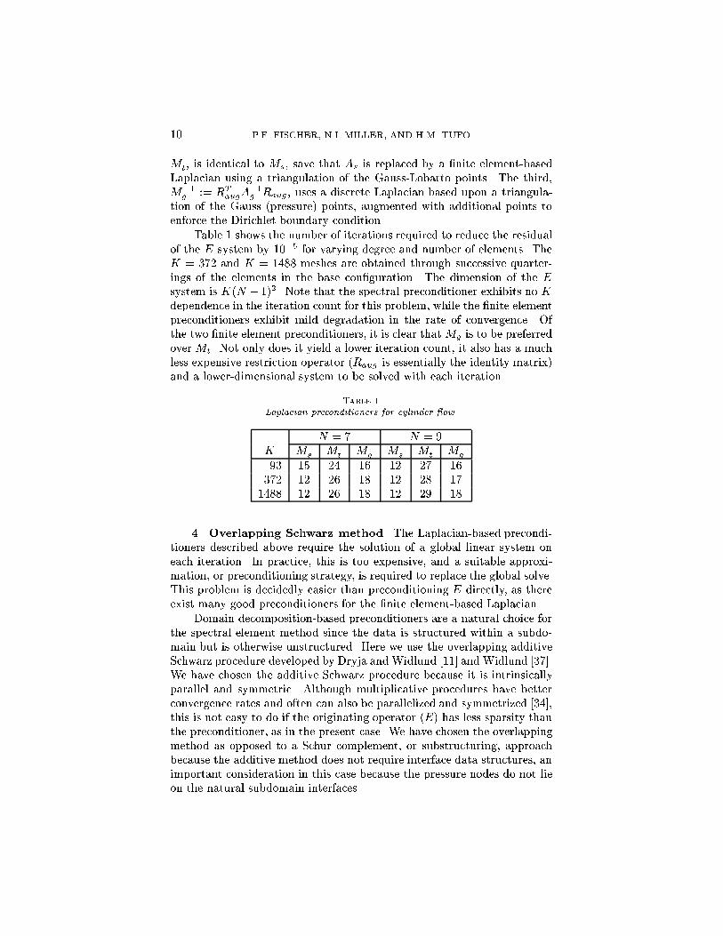
10 P.F. FISCHER, N.I. MILLER, AND H.M. TUFOMt, is identical to Ms, save that As is replaced by a �nite element-basedLaplacian using a triangulation of the Gauss-Lobatto points. The third,M�1g := RTaugA�1g Raug , uses a discrete Laplacian based upon a triangula-tion of the Gauss (pressure) points, augmented with additional points toenforce the Dirichlet boundary condition.Table 1 shows the number of iterations required to reduce the residualof the E system by 10�5 for varying degree and number of elements. TheK = 372 and K = 1488 meshes are obtained through successive quarter-ings of the elements in the base con�guration. The dimension of the Esystem is K(N � 1)2. Note that the spectral preconditioner exhibits no Kdependence in the iteration count for this problem, while the �nite elementpreconditioners exhibit mild degradation in the rate of convergence. Ofthe two �nite element preconditioners, it is clear thatMg is to be preferredover Mt. Not only does it yield a lower iteration count, it also has a muchless expensive restriction operator (Raug is essentially the identity matrix)and a lower-dimensional system to be solved with each iteration.Table 1Laplacian preconditioners for cylinder ow.N = 7 N = 9K Ms Mt Mg Ms Mt Mg93 15 24 16 12 27 16372 12 26 18 12 28 171488 12 26 18 12 29 184. Overlapping Schwarz method. The Laplacian-based precondi-tioners described above require the solution of a global linear system oneach iteration. In practice, this is too expensive, and a suitable approxi-mation, or preconditioning strategy, is required to replace the global solve.This problem is decidedly easier than preconditioning E directly, as thereexist many good preconditioners for the �nite element-based Laplacian.Domain decomposition-based preconditioners are a natural choice forthe spectral element method since the data is structured within a subdo-main but is otherwise unstructured. Here we use the overlapping additiveSchwarz procedure developed by Dryja and Widlund [11] and Widlund [37].We have chosen the additive Schwarz procedure because it is intrinsicallyparallel and symmetric. Although multiplicative procedures have betterconvergence rates and often can also be parallelized and symmetrized [34],this is not easy to do if the originating operator (E) has less sparsity thanthe preconditioner, as in the present case. We have chosen the overlappingmethod as opposed to a Schur complement, or substructuring, approachbecause the additive method does not require interface data structures, animportant consideration in this case because the pressure nodes do not lieon the natural subdomain interfaces.

SCHWARZ METHODS FOR SPECTRAL ELEMENTS 11Formally, the additive Schwarz preconditioner is expressed as the sumof outputs from several subproblems:M�1o = RT0 A�10 R0 + KXk=1RTkA�1k Rk :The subproblems for k � 1 correspond to the solution of local Poissonproblems on overlapping subdomains, ~k. The restriction and prolonga-tion operators, Rk and RTk , k � 1, are Boolean matrices that transfer datato and from the subdomain problems. The product pk = Rkp extracts thecomponents of a vector p which belong to ~k, while p = RTk pk copies thecomponents of a subdomain solution, pk, to a global vector, p, and setscomponents outside of ~k to zero. In addition to the local problems, theSchwarz preconditioner has a coarse grid component, denoted here by sub-script 0, which serves to e�ciently eliminate low-wave number componentsof the residual. The coarse grid problem corresponds to a Poisson problemdiscretized on a mesh de�ned by a triangulation of the subdomain vertices.The prolongation operator, RT0 , is simply an interpolant from the coarsegrid to the Gauss points. @ ~k�?kq q qq q qq q b� q q qq q qb b b q q qq q qq qb�q qq qq q bbb b b bb b bb b b bbb q qq qq qq qq q qq q qb� b b bq q qq q q q qq q qq q qb�Fig. 3. Degrees-of-freedom (open circles) for FEM based (left) and tensor-productbased (right) discretizations of local problems. Values at nodes marked \" are set tozero by Rk. Zero Dirichlet boundary conditions are applied on @ ~k.4.1. FDM application to the subdomain problems. In this sec-tion we consider the development of solvers for the local problems thatare particularly well suited to the spectral element method in lR3. Ratherthan working with principal submatrices of Ag as in [17], we derive the lo-cal sti�ness matrices, Ak, k � 1, from a tensor-product of one-dimensional�nite element bases. This di�erence in strategy is re ected in Fig. 3, whichcontrasts the previous unstructured �nite element (FEM) basis on the leftwith the structured tensor-product basis on the right. This allows the use

12 P.F. FISCHER, N.I. MILLER, AND H.M. TUFOof FDM-based solvers, which require only O(Nd) storage and O(Nd+1)work per solve [7, 8, 31]. An added bene�t is the avoidance of having totetrahedralize the Gauss points in lR3.We begin with the de�nition of the overlapping subdomains by con-sidering the one-dimensional example shown in Fig. 4. Degrees-of-freedomare associated with the nodes (open circles) in ~k. The points �i, i 2f1; : : : ; N � 1g are the images of the Gauss points in ]� 1; 1[ mapped ontok. Similarly, �i, i � 0 and i � N are the images of the correspondingGauss points mapped onto the left and right subdomains, respectively. Theoverlapping region, ~k 2 [��1; �N+1], is obtained by extending k by twonodal points in each direction. Homogeneous Dirichlet boundary condi-tions are applied at ��1 and �N+1 when k is in the interior of so theextension adds only two degrees-of-freedom to the local problem. We referto this as the minimal overlap case. If the left (right) side of @k is co-incident with the boundary, @, then the domain is not extended beyond 0 ( N ), and homogeneous Dirichlet or Neumann boundary conditions areimposed at that point in accordance with the boundary conditions on @.d d d d�1 �2 �N�2 �N�1 0 N� k -� ~k -t d��1 �0� - d t�N �N+1� +Fig. 4. Depiction of overlapping subdomain ~k in one dimension, minimal overlapcase.To construct the �nite element operators for the standard (interior)one-dimensional case, we consider the space of piecewise linear functions,�i(�), � 2 [��1; �N+1], i = 0; : : : ; N :�i(�) = 8>>>>>><>>>>>>: � � �i�1�i � �i�1 �i�1 � � < �i� � �i+1�i � �i+1 �i � � < �i+10 otherwise: i 2 f0; : : : ; Ng(4.1)The variational form for the homogeneous Dirichlet problem, �u00(x) =f(x) in ~k, u = 0 on ~@k, gives rise to the tridiagonal sti�ness matrix:~Aij = Z �N+1��1 d�id� d�jd� d� i; j 2 f0; : : : ; Ng2 ;

SCHWARZ METHODS FOR SPECTRAL ELEMENTS 13and associated diagonal (lumped) mass matrix:~Bij = �ij Z �N+1��1 �j(�)d� i; j 2 f0; : : : ; Ng2 :The matrices are modi�ed in the usual way if either end of k coincideswith @.The construction of the one-dimensional problem is extended to lRdby taking the tensor product of the bases and operators just described. Atypical overlapping domain in lR2 is shown in Fig. 3 (right). The degrees-of-freedom correspond to Lagrangian basis coe�cients associated with thenodes (open circles) in the interior of ~k. If the nodes are numbered lexi-cographically, then the sti�ness matrix for the two-dimensional Laplacianon ~k can be written as the Kronecker product:Ak = ~B2 ~A1 + ~A2 ~B1 :(4.2)Here, the subscript on the one-dimensional matrices, ~A and ~B, indicatesthe associated coordinate direction in the reference element.Matrices that satisfy (4.2) have a particularly simple inverse basedupon the FDM. If ~A is symmetric and ~B is symmetric positive de�nite,then the following similarity transformation holds:ST ~AS = �; ST ~BS = I;where � = diag(�1; : : : ; �n) the matrix of eigenvalues, and S = (s1; : : : ; sn)is the matrix of eigenvectors associated with the generalized eigenvalueproblem ~As = � ~Bs. As a result, Ak is readily diagonalized, and its inverseis given by A�1k = (S2 S1) (I �1 + �2 I)�1 (ST2 ST1 ) :The three-dimensional form is similar:A�1k = (S3 S2 S1)D�1(ST3 ST2 ST1 ) ;with D = (I I �1 + I �2 I +�3 I I):This solution method was introduced by Lynch, Rice, and Thomas [31] andsuccessfully used in a number of spectral element preconditioning applica-tions by Couzy and Deville [8] and by Couzy [7].It is important to note that the use of tensor-product forms allowsmatrix-vector products, to be recast as matrix-matrix products which areparticularly e�cient on modern vector and cache-based processors. For ex-ample, if ~uk = ukij , i; j 2 f0; : : : ; Ng2 is the vector of nodal basis coe�cientson ~k, then

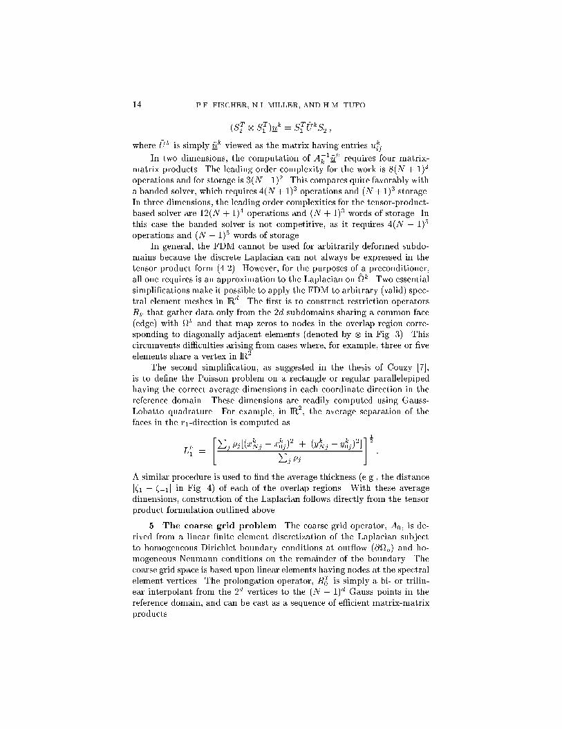
14 P.F. FISCHER, N.I. MILLER, AND H.M. TUFO(ST2 ST1 )uk = ST1 ~UkS2 ;where ~Uk is simply ~uk viewed as the matrix having entries ukij .In two dimensions, the computation of A�1k ~uk requires four matrix-matrix products. The leading order complexity for the work is 8(N + 1)3operations and for storage is 3(N+1)2. This compares quite favorably witha banded solver, which requires 4(N+1)3 operations and (N +1)3 storage.In three dimensions, the leading order complexities for the tensor-product-based solver are 12(N + 1)4 operations and (N + 1)3 words of storage. Inthis case the banded solver is not competitive, as it requires 4(N + 1)5operations and (N + 1)5 words of storage.In general, the FDM cannot be used for arbitrarily deformed subdo-mains because the discrete Laplacian can not always be expressed in thetensor product form (4.2). However, for the purposes of a preconditioner,all one requires is an approximation to the Laplacian on ~k. Two essentialsimpli�cationsmake it possible to apply the FDM to arbitrary (valid) spec-tral element meshes in lRd. The �rst is to construct restriction operatorsRk that gather data only from the 2d subdomains sharing a common face(edge) with k and that map zeros to nodes in the overlap region corre-sponding to diagonally adjacent elements (denoted by in Fig. 3). Thiscircumvents di�culties arising from cases where, for example, three or �veelements share a vertex in lR2.The second simpli�cation, as suggested in the thesis of Couzy [7],is to de�ne the Poisson problem on a rectangle or regular parallelepipedhaving the correct average dimensions in each coordinate direction in thereference domain. These dimensions are readily computed using Gauss-Lobatto quadrature. For example, in lR2, the average separation of thefaces in the r1-direction is computed asLk1 = "Pj �j [(xkNj � xk0j)2 + (ykNj � yk0j)2]Pj �j # 12 :A similar procedure is used to �nd the average thickness (e.g., the distancej�1 � ��1j in Fig. 4) of each of the overlap regions. With these averagedimensions, construction of the Laplacian follows directly from the tensorproduct formulation outlined above.5. The coarse grid problem. The coarse grid operator, A0, is de-rived from a linear �nite element discretization of the Laplacian subjectto homogeneous Dirichlet boundary conditions at out ow (@o) and ho-mogeneous Neumann conditions on the remainder of the boundary. Thecoarse grid space is based upon linear elements having nodes at the spectralelement vertices. The prolongation operator, RT0 is simply a bi- or trilin-ear interpolant from the 2d vertices to the (N � 1)d Gauss points in thereference domain, and can be cast as a sequence of e�cient matrix-matrixproducts.

SCHWARZ METHODS FOR SPECTRAL ELEMENTS 15In two dimensions, the quadrilateral spectral element mesh is readilytriangulated by connecting one pair of diagonally opposing vertices in eachof the elements. In three dimensions, an equivalent local procedure is com-plicated by the fact that the tetrahedral decomposition of a cube introducesa diagonal on each face, which must match the direction of the diagonalintroduced on the face of the adjoining cube for the resulting discretiza-tion to be conforming. The tessellation problem in lR3 can be localized bycomputing the (local) sti�ness matrices for the two complementary tetrahe-dralizations of the reference cube shown on the left in Fig. 5. If A0 and A00denote the global matrices obtained by assembling compatible sets of localsti�ness matrices, then A0 := 12 (A0 +A00) is the global sti�ness matrix onewould obtain by taking the average of two conforming sti�ness matrices.However, A0 can be constructed without solving the nonlocal problem ofdetermining a conforming tetrahedralization by simply assembling the localsti�ness matrices of all ten tetrahedra de�ned by the two complementarydecompositions.[ �!Fig. 5. The symmetric union of two complementary decompositions of the referencecube localizes the problem of �nding a conforming coarse grid space.5.1. Parallel coarse grid solver. Solution of the coarse grid prob-lem has long been recognized as a bottleneck in parallel applications wherecommunication costs are non-negligible, such as on networks of worksta-tions or when the number of processors is large (see, e.g., [2, 12, 22, 34]).Since A�10 is full, each coarse grid solve requires an all-to-all communica-tion, as every entry of the distributed input has a nontrivial impact onevery output value. Assuming that each processor is capable of sending orreceiving only one message at a time and that contention-free communi-cation time for an m-word message obeys a linear cost model of the formtc[m] = � + �m, then the minimum time for solution of the distributedcoarse grid problem is � log2 P . It is typically best to use a contention-freerouting schedule, which implies a minimum time of 2� log2 P for standardschedules on low-dimensional networks.As noted by Gropp in [19], most parallel solvers for an n�n coarse gridproblem require log2 P messages of length n for each solve. Since n > P ,this can become prohibitive if either � or P is large. We have recentlydeveloped a parallel coarse grid solver with a communication complexityof only O(n 12�log2P ) in lR2 and O(n 23�log2P ) in lR3 [16, 36]. The solver

16 P.F. FISCHER, N.I. MILLER, AND H.M. TUFOderives from the observation that projection of a distributed vector onto adistributed basis is naturally parallel.Let A0x = b denote the n � n coarse grid system to be solved, withb and x identically distributed across processors at the beginning and endof the solution phase. If X = (x1; : : : ; xl) 2 lRn�l is a matrix of A0{orthonormal vectors satisfying xTi A0xj = �ij , then the projection of x ontospanfx1; : : : ; xlg is given by �x = XXT b. If the xi's are mapped in the samemanner as x and b, then parallel evaluation of �x on P processors involvesthree steps:i: �(p)i = �x(p)i �T b(p) i = 1; : : : ; l p = 0; : : : ; P�1ii: �i = Xp �(p)i i = 1; : : : ; liii: �x(p) = Xi �ix(p)i p = 0; : : : ; P�1 :(5.1)Here, the superscript (p) indicates the processor index for distributed data.Step (ii) is an interprocessor vector-reduction and can be computed viaa fan-in/fan-out on a binary tree in 2 log2 P communication phases withmessages of length l.Note that if l = n, then �x � x, and the projection produces the exactsolution. If A0 is sparse, it is possible to choose a (quasi-) sparse basis forXsuch that many of the xi's are void on any given processor. This implies areduction in communication as well as work since the corresponding valuesof �i are not needed by all processors. For low-order discretizations in lRdit is possible to choose the columns of X such that it has only O(n 2d�1d )nonzeros and such that only log2 P messages of length O(n d�1d ) are requiredto compute XXT b. Further details may be found in [36].We note that the vertex-based coarse grid problems such as consideredhere nominally require communication in the restriction and prolongationsteps because each vertex may be shared by many processors. These extracommunications can be avoided by embedding them directly into the XXTcomputation. Let z := RT0 A�10 R0r, denote the full coarse grid problem.Consider the factorization: R0 = QT0QTPITP ;where IP represents the local interpolation from the subdomain verticesto the Gauss points, QTP represents the direct-sti�ness summation (or as-sembly of the load vector) of vertex values within each processor, and QT0represents the interprocessor direct-sti�ness summation step. Only the ap-plication of Q0 (QT0 ) requires communication. Writing X0 := XQ0, wehave z = (IPQP )X0XT0 �QTPITP r� :

SCHWARZ METHODS FOR SPECTRAL ELEMENTS 17This corresponds to computing a projection of the form x0 = X0XT0 b0and is identical in complexity to (5.1) on an enlarged vector space. Nopre- or post-communication is required during the coarse grid solve, sinceapplication of (IPQP ) is local. All communication is embedded in thelog2 P fan-in/fan-out stage (5.1.ii) of X0XT0 b0.6. Numerical results. We compare the results of the FDM-basedadditive Schwarz method to the results of the FEM-based additive Schwarzpreconditioner [17] and the block-Jacobi/de ation-based scheme developedin [15, 32].6.1. Two-dimensional cylinder problem. We �rst consider thecylinder problem of Fig. 2. The conditions are the same as those used inthe Laplacian preconditioning tests of Section 3.1 save that we restrict thepolynomial order to N = 7. Table 2 shows the iteration count and CPUtimes for the FDM-based additive Schwarz procedure with minimal overlap.Also shown are the iteration counts and times for the additive Schwarzprocedure based upon the unstructured FEM discretization where the localsti�ness matrices, Ak, k � 1, are principal submatrices of Ag . The No = 0column corresponds the the FEM scheme with no overlap. Introducinga minimal amount of overlap (No = 1) reduces the iteration count almosttwofold and the CPU time slightly less than twofold. Increasing the overlapto No = 3 does not yield signi�cant improvement. The importance of thecoarse grid solve is illustrated by the A0 = 0 column, which shows a �ve- toeightfold increase in iteration count for the K = 1488 case when the coarsegrid solver is excluded. The �nal column shows the performance of ourde ation-based production code [15]. It requires roughly twice the numberof iterations as the FDM scheme and almost three times the CPU time.(The de ation approach requires two applications of E per iteration.)Table 2Performance of the additive Schwarz algorithm.FDM No = 0 No = 1 No = 3 A0 = 0 De ationK iter cpu iter cpu iter cpu iter cpu iter cpu iter cpu93 67 4.4 121 10 64 5.9 49 5.6 169 19 126 17372 114 37 203 74 106 43 73 39 364 193 216 1251488 166 225 303 470 158 274 107 242 802 1798 327 845We note that, because of the use of the approximate Laplacians, theFDM-based scheme has a slightly higher iteration count than the FEMscheme in the minimal overlap case (No = 1). Despite this and despite itshigher complexity estimate (8K(N + 1)3 vs 4K(N + 1)3) the FDM-basedscheme requires less time. This clearly illustrates the importance of thematrix-matrix product-based solution algorithm.Somewhat disappointingly, the iteration counts for the overlappingSchwarz method are not bounded with K. Our experience indicates that

18 P.F. FISCHER, N.I. MILLER, AND H.M. TUFOthe iteration count does eventually approach a bound, but only after manylevels of re�nement. We have investigated two possible solutions. The �rst,suggested by Widlund [38], is to use more overlap on the (few) subdomainswhich have high aspect ratio. This reduces the iteration count while main-taining low CPU time [17]. The second is use of nonconforming spectralelement methods, which remove these high aspect ratio subdomains alto-gether. As demonstrated by G. Kruse [20], this results in signi�cantly loweriteration counts.6.2. Three-dimensional hemisphere problem. We now considerparallel simulation of the three-dimensional ow arising from the interac-tion of a at plate boundary layer with a hemispherical protuberance. This ow was studied experimentally by Acalar and Smith [1] and, at su�cientlyhigh Reynolds numbers, exhibits periodic shedding of hairpin vortices asevinced by the isotherms in the centerplane of the channel shown in Fig. 6.The unit radius hemisphere is centered at x = (0; 0; 0), and the Reynoldsnumber is Re = RU1� = 500. A Blasius pro�le with �:99 = 1:15 and U1 = 1is speci�ed for the x-component of velocity both as an initial condition andinlet pro�le at x = �8:4. Symmetry boundary conditions are speci�ed aty = 0, y = �6:4, and z = 6:5, and Neumann out ow boundary conditionsare imposed at x = 25:6. Discretizations consisting of K = 512 and 4096spectral elements of order N = 7, 9, and 11 are considered for a �xed timestep of �t = 0:00636. Timings are performed on the P = 512 node In-tel Delta at Caltech, which is a mesh connected multicomputer based on512 Intel i860 40 MHz microprocessors, each with 16 Mbytes of memory.Sustained performance on this machine for these runs is typically about 5gflops in 32-bit arithmetic.Fig. 6. Isotherms reveal the presence of hairpin vortices generated by the interac-tion of a at-plate boundary later with a (heated) hemisphere in this (K = 4096; N = 7)spectral element simulation.In Fig. 7 we show the CPU time per step for the de ation- and FDM-based computations with (K;N) = (512; 11) and (4096,9). A good initialguess, computed from an orthogonal projection of the data onto previ-ous solutions, signi�cantly reduces the iteration count after the �rst fewtime steps, so the performance at later times is most representative of theasymptotic behavior of the solvers during the course of the simulation [14].

SCHWARZ METHODS FOR SPECTRAL ELEMENTS 19se

cond

s

step number

Deflation

Schwarz10.00

20.00

30.00

40.00

50.00

60.00

70.00

80.00

90.00

5.00 10.00 15.00

seco

nds

step number

Deflation

Schwarz100.00

200.00

300.00

400.00

500.00

600.00

5.00 10.00 15.00Fig. 7. 512-node CPU time for the �rst 19 steps of the hemisphere problem for(K;N) = (512; 11) (left) and (4096; 9) (right).Table 3 shows the number of pressure iterations and CPU time required forthe 19th step. We observe that the overlapping Schwarz procedure yields athree- to �vefold reduction in iteration count over the de ation scheme anda fourfold improvement in CPU time for the largest problem. The fact thatthe CPU-time reduction is less than that of the iteration count shows thatthe overlapping Schwarz procedure has e�ectively eliminated the pressuresolve as the computational bottleneck for this class of problems. In fact, itis now on par with the cost of the Helmholtz solves.Table 3Timing for hemisphere/plate problem on 512 node Delta.De ation SchwarzK N # vel. pts. # pres. pts. iter cpu iter cpu512 7 179000 111000 19 5.3 4 3.2512 9 380000 262000 27 8.8 5 4.7512 11 693000 512000 36 15.8 13 8.14096 7 1423000 884000 78 58.4 20 18.24096 9 3016000 2097000 137 143.0 26 36.7We examine the importance of the XXT -based coarse grid solver viadirect comparison to the same overlapping Schwarz code modi�ed to use adistributed A�1-based solver. The latter has O(n log2 P ) communicationcomplexity for each coarse grid solve, versus the O(n 23 log2 P ) complexityof the XXT based solver. For K = 512 the dimension of the coarse gridsystem is n = 781, while for K = 4096 it is n = 5114. Table 4 indicates thepercentage of overall solution time spent in the coarse grid solver as well asthe time per coarse grid solve for both cases. For the K = 4096 data, there

20 P.F. FISCHER, N.I. MILLER, AND H.M. TUFOis a 12 and 9 percent reduction in overall solution time due to the use ofXXT based solver. In addition, there is fourfold improvement in the timeper coarse grid solve for n = 5114, and twofold for n = 781. We note thatthis is consistent with predictions based on the theoretical models for bothsolvers discussed in [36]. Table 4Coarse grid costs for hemisphere/plate problem on 512 node Delta.A�1 Method XXT MethodK N # d.o.f. % time sec./slv. % time sec./slv.512 7 781 4.82 0.021 2.66 0.011512 9 781 5.32 0.021 3.03 0.011512 11 781 5.38 0.021 3.08 0.0124096 7 5114 16.4 0.091 4.26 0.0214096 9 5114 12.6 0.094 3.45 0.0237. Conclusions. We have developed an overlapping Schwarz precon-ditioner for the pressure subproblem in time-split spectral element formu-lations of the incompressible Navier-Stokes equations that is particularlye�cient for problems in three dimensions. The method employs tensor-product discretizations for the local subdomain problems that admit so-lution via fast diagonalization techniques having the same computationalcomplexity as the originating spectral element operators, and that are read-ily implemented within the locally structured context of the spectral ele-ment method. The parallel performance of the method is enhanced by afast coarse grid solve algorithm that has signi�cantly better communica-tion complexity than competing approaches. In comparison to our earlierblock-Jacobi/de ation based production code, we observe a �vefold reduc-tion in iteration count and, for the largest problems, a fourfold reductionin CPU time. The overlapping Schwarz preconditioner has e�ectively elim-inated the pressure solve as a computational bottleneck. It now becomesimportant to consider whether the other phases of the solution process canbe further improved.Acknowledgments. This work was supported by the NSF underGrant ASC-9405403 and by the AFOSR under Grant F49620-95-1-0074.Computer time was provided on the Intel Delta at Caltech by the Centerfor Research on Parallel Computation under NSF Cooperative agreementCCR-8809615.

SCHWARZ METHODS FOR SPECTRAL ELEMENTS 21REFERENCES[1] M.S. Acalar and C.R. Smith, \A study of hairpin vortices in a laminar bound-ary layer. Part 1. Hairpin vortices generated by a hemisphere protuberance",J. Fluid Mech., 175, pp. 1{41 (1987).[2] F. Alvarado, A. Pothen, and R. Schreiber, \Highly parallel sparse triangularsolution", Univ. Waterloo Research Rep. CS-92-51, Waterloo, Ontario (1992).[3] C. Bernardi and Y. Maday, \A collocation method over staggered grids for theStokes problem", Int. J. Numer. Meth. Fluids, 8, pp. 537{557 (1988).[4] J. Blair Perot, \An analysis of the fractional step method", J. Comput. Phys.,108, pp. 51{58 (1993).[5] M. Casarin, \Quasi-optimal Schwarz methods for the conforming spectral elementdiscretization", Tech.Rep. 705, Dept. Comp. Sci., Courant Inst., NYU (1995).[6] M. Casarin, \Schwarz preconditioners for spectral and mortar �nite element meth-ods with applications to incompressible uids", PhD. Thesis, Courant Instituteof Math. Sci., NYU (1996).[7] W. Couzy, \Spectral element discretization of the unsteady Navier-Stokes equa-tions and its iterative solution on parallel computers", Th�ese No. 1380, �EcolePolytechnique F�ed�erale de Lausanne (1995).[8] W. Couzy and M.O. Deville, "A Fast Schur Complement Method for the Spec-tral Element Discretization of the Incompressible Navier-Stokes Equations",J. Comput. Phys., vol. 116, pp. 135{142 (1995).[9] P. Demaret and M.O. Deville, \Chebyshev pseudo-spectral solution of theStokes equations using �nite element preconditioning", J. Comput. Phys., 83,pp. 463{484 (1989).[10] M.O. Deville and E.H. Mund, \Finite element preconditioning for pseudospec-tral solutions of elliptic problems", SIAM J. Statis. Comput., 11(2), pp. 311{42 (1990).[11] M. Dryja and O.B. Widlund, \An additive variant of the Schwarz alternatingmethod for the case of many subregions", Tech. Rep. 339, Dept. Comp. Sci.,Courant Inst., NYU (1987).[12] C. Farhat and P.S. Chen, \Tailoring Domain Decomposition Methods for E�-cient Parallel Coarse Grid Solution and for Systems with Many Right HandSides", Contemporary Math., 180, pp. 401{406 (1994).[13] P.F. Fischer, \Spectral Element Solution of the Navier-Stokes Equations on HighPerformance Distributed-Memory Parallel Processors", PhD. Thesis, Mas-sachusetts Institute of Technology (1989).[14] P.F. Fischer, \Projection techniques for iterative solution of Ax = b with succes-sive right-hand sides", ICASE Report No. 93-90, NASA CR-191571 (1993).[15] P.F. Fischer and E.M. R�nquist, \Spectral Element Methods for Large ScaleParallel Navier-Stokes Calculations", Comp. Meth. Appl. Mech. Engr., pp. 69{76 (1994).[16] P.F. Fischer, \Parallel multi-level solvers for spectral element methods", in Proc.Intl. Conf. on Spectral and High-Order Methods '95, Houston, TX, A.V. Ilinand L.R. Scott, eds., Houston J. Math., pp. 595-604 (1996).[17] P.F. Fischer, \An overlapping Schwarz method for spectral element solution ofthe incompressible Navier-Stokes equations", J. of Comp. Phys., 133, pp. 84{101 (1997).[18] N.K. Ghaddar, K. Korczak, B.B. Mikic, and A.T. Patera, \Numerical in-vestigation of incompressible ow in grooved channels. Part 1: Stability andself-sustained oscillations", J. Fluid Mech., 163, pp. 99{127 (1986).[19] D.E. Keyes, Y. Saad, and D.G. Truhlar, \Domain-Based Parallelism andProblem Decomposition Methods in Computational Science and Engineering",SIAM (1995).[20] G.W. Kruse, \Parallel Nonconforming Spectral Element Solution of the Incom-pressible Navier-Stokes Equations in Three Dimensions", PhD. Thesis, BrownUniversity (1997).

22 P.F. FISCHER, N.I. MILLER, AND H.M. TUFO[21] V. Girault and P.A. Raviart, Finite Element Approximation of the Navier-Stokes Equations, Springer (1986).[22] W.D. Gropp, \Parallel Computing and Domain Decomposition", in Fifth Conf.on Domain Decomposition Methods for Partial Di�erential Equations, T.F.Chan, D.E. Keyes, G.A. Meurant, J.S. Scroggs, and R.G. Voigt, eds., SIAM,Philadelphia, PA, pp. 349{361 (1992).[23] Y. Maday and A.T. Patera, \Spectral element methods for the Navier-Stokesequations", in State of the Art Surveys in Computational Mechanics, A.K.Noor, ed., ASME, New York, pp. 71{143 (1989).[24] Y. Maday, A.T. Patera, and E.M. R�nquist, \An operator-integration-factorsplitting method for time-dependent problems: application to incompressible uid ow", J. Sci. Comput., 5(4), pp. 263{292 (1990).[25] Y. Maday, A.T. Patera, and E.M. R�nquist, \The PN �PN�2 method for theapproximation of the Stokes problem", Numer. Math. (1987).[26] S.A. Orszag and L.C. Kells, \Transition to turbulence in plane Poiseuille owand plane Couette ow", J. Fluid Mech., 96, pp. 159{205 (1980).[27] S.A. Orszag, \Spectral methods for problems in complex geometries", J. Comput.Phys., 37, pp. 70{92 (1980).[28] S.S. Pahl, \Schwarz type domain decomposition methods for spectral elementdiscretizations", Masters Thesis, Dept. of Comput. and Appl. Mathematics,Univ. of the Witwatersrand, Johannesburg, South Africa (1993).[29] A.T. Patera, \A spectral element method for uid dynamics; Laminar ow in achannel expansion", J. Comput. Phys., 54, pp. 468{488 (1984).[30] L.F. Pavarino and O.B. Widlund, \A polylogarithmic bound for an iterativesubstructuring method for spectral elements in three dimensions", SIAM J.Numer. Anal., 33(4), pp. 1303{1335 (1996).[31] R.E. Lynch, J.R. Rice, and D.H. Thomas, \Direct Solution of Partial Di�erenceEquations by Tensor Product Methods", Numerische Mathematik, 6, pp. 185{199 (1964).[32] E.M. R�nquist, \A Domain Decomposition Method for Elliptic Boundary ValueProblems: Application to Unsteady Incompressible Fluid Flow", in Fifth Conf.on Domain Decomposition Methods for Partial Di�erential Equations, T.F.Chan, D.E. Keyes, G.A. Meurant, J.S. Scroggs, and R.G. Voigt, eds., SIAM,Philadelphia, PA, pp. 545{557 (1992).[33] E.M. R�nquist, \A domain decomposition solver for the steady Navier-Stokesequations", in Proc. Intl. Conf. on Spectral and High-Order Methods '95,Houston, TX, A.V. Ilin and L.R. Scott, eds., pp. 469{485 (1996).[34] B. Smith, P. Bj�rstad, and W. Gropp, \Domain Decomposition", CambridgeUniversity Press, 1996.[35] G. Strang and G. Fix, An analysis of the �nite element method, Prentice-Hall,Englewood Cli�s, NJ (1973).[36] H.M. Tufo and P.F. Fischer, \Fast Parallel Direct Solvers For Coarse GridProblems", prepared (1997).[37] O.B. Widlund, \Some Schwarz Methods for Symmetric and Nonsymmetric Ellip-tic Problems", in Fifth Conf. on Domain Decomposition Methods for PartialDi�erential Equations, T.F. Chan, D.E. Keyes, G.A. Meurant, J.S. Scroggs,and R.G. Voigt, eds., SIAM, Philadelphia, PA, pp. 19{36 (1992).[38] O.B. Widlund, Personal communication (1997).