The Pennsylvania State University

The Graduate School

College of Engineering

AN FPGA BASED REAL-TIME TRACKING SYSTEM FOR

INDOOR ENVIRONMENTS

A Thesis in

Electrical Engineering

by

Vikram Sampath Kumar

2010 Vikram Sampath Kumar

Submitted in Partial Fulfillment

of the Requirements for the Degree of

Master of Science

May 2010

The thesis of Vikram Sampath Kumar was reviewed and approved* by the following:

Vijaykrishnan Narayanan

Professor of Computer Science and Engineering Thesis Advisor

Suman Datta Associate Professor of Electrical Engineering

Thesis Co-Advisor

Kenneth .W. Jenkins

Professor of Electrical Engineering Head of the Department of Electrical Engineering

*Signatures are on file in the Graduate School

iii

ABSTRACT

Advanced Human Computer Interfacing has become an active field of research in a very

short span since its inception. Computing systems need to be built in such a way that they can

interact with humans at human interaction speeds. Face Detection and Pedestrian Tracking are

few such applications that highlight this fact. A real-time tracking system must be able to track

the movement of a person or multiple persons within the field of view of a video camera. The

system must exhibit a level of robustness that maintains accuracy and performance in dynamic

environments that include multiple occlusions, changing scenery, light intensity variations, and

shadows. Additionally, tracking systems may extract details such as shirt/face color, age, and

height of persons that have been successfully tracked over a number of frames. The goal is to

perform all such tasks in real time at frame rates of at least 30 frames per second. Moreover,

small form factor is often a requirement in applications in which the image/video processing must

be performed on-site in a non-obtrusive fashion. Smart Cameras are embedded with small FPGAs

that can process images on-the-go. For instance, such a system finds great use in building home-

care systems for monitoring elderly people in their homes when they are alone. The response time

and the size of the system are very vital.

This thesis describes an FPGA implementation of a tracking system that gives excellent

performance benefits when compared to analogous software implementations on a general

purpose processor. The system consists of streaming image processing components which are

ideally suited for tracking applications.

iv

TABLE OF CONTENTS

LIST OF FIGURES………………………………………………………………….vii

LIST OF TABLES…………………………………………………………………....ix

ACKNOWLEDGEMENTS…………………………………………………………..x

Chapter 1 INTRODUCTION TO TRACKING…………………………………….1

1.1 Applications of Object Tracking…………………………………………..1

1.2 Problems Associated with Object Tracking…………………………..........2

Chapter 2 TRACKING BACKGROUND……………………………………….......3

2.1 Object Representation……………………………………………………. .3

2.2 Feature Selection…………………………………………………………...3

2.3 Object Detection…………………………………………………………....4

2.3.1 Background Subtraction………………………………………....5

2.3.2 Segmentation………………………………………………….....6

2.3.3 Association……………………………………………………....7

Chapter 3 BACKGROUND ESTIMATION………………………………………...8

3.1 Implementation…………………………………………………………….8

3.1.1 Training Phase…………………………………………………..9

3.1.2 Estimation Phase………………………………………………..11

3.1.3 Hardware Implementation of 8x8 Filter………………………...15

Chapter 4 CONNECTED COMPONENT LABELING…………………………....18

4.1 Related Work……………………………………………………………....19

v

4.2 Single Pass Algorithm……………………………………………………...19

4.2.1 Pixel Buffer……………………………………………………...21

4.2.2 End of Box Detection……………………………………………22

4.3 Sliced Single Pass Algorithm………………………………………………24

4.3.1 Algorithm Motivation and Overview……………………………25

4.3.2 Connected Component Processor………………………………..26

4.3.3 Slice Processor…………………………………………………...26

4.3.4 Coalescing Unit…………………………………………………..27

4.3.5 Functions of the Slice Processor…………………………………28

4.3.6 Enqueueing the Association FIFO……………………………….30

4.3.7 Dequeueing the Association FIFO…………………………….....32

4.3.8 Common Label (CL) RAMs……………………………………...34

4.3.9 Updating Global Bounding Box RAM…………………………...35

4.3.10 Bounding Box Update…………………………………………..35

4.3.11 Results…………………………………………………………..36

Chapter 5 INTEGRAL IMAGE……………………………………………………….39

5.1 Algorithm Overview………………………………………………………...39

5.2 Implementation……………………………………………………………...40

Chapter 6 TRACKING UNIT………………………………………………………....42

6.1 Discussion…………………………………………………………………...42

6.2 Tracking Algorithm…………………………………………………………43

6.3 Implementation……………………………………………………………...45

6.3.1 Person Detection………………………………………………….46

6.3.2 Centroid Processing Unit…………………………………………47

6.3.3 Current Block……………………………………………………..48

vi

6.3.4 Integral Receive/Transmit………………………………………..48

6.3.5 Update Unit………………………………………………………49

Chapter 7 CONCLUSION……………………………………………………………..53

REFERENCES………………………………………………………………………….54

vii

LIST OF FIGURES

Figure 2-1: (a) Bounding Box (b) Contour (c) Ellipse (d) Skeleton (e) Articulated

(f) Centroid – Object Representation. ............................................................... 3

Figure 2-2: Background Subtraction . ................................................................................ 5

Figure 2-3: Segmentation (Connected Components Analysis). ............................................ 6

Figure 3-1: Hardware Implementation of Training Phase in Background

Subtraction………………………………………………………………………10

Figure 3-2: Hardware Implementation of Estimation Phase in Background

Subtraction………………………………………………………………………12

Figure 3-3: Background Subtraction Illustration Background Frame (top);

Current Frame(middle); Background Subtraction (bottom)……………………13

Figure 3-4: A 4x4 Filter Illustration……………………………………………………….14

Figure 3-5: Hardware Implementation of 8x8 Filter………………………………………...16

Figure 3-6: (a) Background Image (b) Current Image (c) Background Subtraction

(d) Background Subtraction with 8x8 Filter……………………………………17

Figure 4-1: Pixel Labeling…………………………………………………………………...20

Figure 4-2: Streaming Single Pass Architecture……………………………………………..22

Figure 4-3: End of Bounding Box Detection………………………………………………...23

Figure 4-4: Sliced Connected Component Labeling Architecture…………………………...24

Figure 4-5: Four Possible Box Completion Scenarios…………………………………….....24

Figure 4-6: Coalescing Unit Architecture……………………………………………………28

Figure 4-7: Slice Processor Functionalities...………………………………………………..30

Figure 4-8: Enqueueing the Association FIFO……………………………………………....31

Figure 4-9: Updating Association FIFO Example…………………………………………...33

viii

Figure 4-10: Execution time as a function of image size (a) proposed architecture

(b) Dual Core Workstation (c) Software implementation on embedded

PowerPC…………………………………………………………………….37

Figure 5-1: ( left) Coordinate representation (centre) Grayscale input image (right)

Corresponding Integral image………………………………………………..39

Figure 5-2: Integral Image Generation Hardware Architecture…………………………...41

Figure 6-1: Tracking Unit Architecture…………………………………………………...45

Figure 6-2: Person Detection Architecture………………………………………………..46

Figure 6-3: Centroid Processing Unit……………………………………………………..47

Figure 6-4: Current Block…………………………………………………………………48

Figure 6-5: Integral Receive/Transmit…………………………………………………….48

Figure 6-6: Update Unit…………………………………………………………………...49

Figure 6-7: A collection of snapshots from a video demo showing every fifth frame……52

ix

LIST OF TABLES

Table 4-1: Updating Association FIFO Example ................................................................. 33

Table 4-2: Comparison with Other Hardware Implementations. ........................................... 38

x

ACKNOWLEDGEMENTS

First, I would like to sincerely thank my advisor Dr.Vijaykrishnan Narayanan for giving

me an opportunity to work in the Microsystems Design Laboratory(MDL). His guidance,

encouragement and support have been invaluable assets during the course of my research. The

research experience I had in MDL has given me an exciting career path to take and I owe this

success to Dr.Vijay.

I would like to thank Dr.Suman Datta, to have agreed to be a part of my committee and

support my thesis work.

I would like to thank all my lab mates at MDL, especially Kevin, for being a great

mentor. Without him, this thesis wouldn‟t have been possible. I would like to extend my thanks to

Ahmed, who has been of tremendous help in my research work.

Finally, I would like to thank my parents and sister Kalpana for their strongest support in

whatever I do. I very sincerely thank Charanya, for handling all the ups and downs I faced over

these years and for her constant motivation, support and love. I also thank all my friends at Penn

State whose company has given fun memories to cherish.

Chapter 1

INTRODUCTION TO TRACKING

Computer Vision is an important research field and among its various tasks, Person

Tracking has generated a great deal of interest. This is partly due to the availability of cheap and

high quality video sensors and the need for automated video analysis in many applications. Any

video analysis algorithm targeted towards object tracking consists of three key steps -

a) Detection of the object of interest in the current frame; b) Tracking of the detected object from

frame to frame; c) Analysis of the tracked object by extracting interesting features.

1.1 Applications of Object Tracking

Yilmaz et.al [1] in their survey mention the pertinent tasks of video analysis algorithms

as listed below:

- motion-based recognition, that is, human identification based on gait, automatic

object detection, etc;

- automated surveillance, that is, monitoring a scene to detect suspicious activities or

unlikely events;

- video indexing, that is, automatic annotation and retrieval of the videos in multimedia

databases;

- human-computer interaction, that is, gesture recognition, eye gaze tracking for data

input to computers, etc.;

- traffic monitoring, that is, real-time gathering of traffic statistics to direct traffic flow;

- vehicle navigation, that is, video-based path planning and obstacle avoidance

2

1.2 Problems associated with Object Tracking

Real world behavior poses many problems to tracking. Addressing each problem is an

extremely challenging task. For instance, illumination changes in the scene affect algorithms that

rely upon color or intensity to perform video analysis. Object shadows, partial and total

occlusion, varying background, and camera jitter are common sources of noise for which the

performance of non-robust tracking schemes will be hindered. Consequently, many algorithms

impose constraints on motion and object appearance to simplify the tracking task.

This thesis describes an implementation of a complete tracking system on an FPGA. The

goal of the tracking system is to identify individuals in a scene and assign a unique id to each. In

addition, the system must track the movement of each person while maintaining a consistent id as

long as the individual is present within the frame. This might involve cases like partial and total

occlusion where the person might be partly or completely hidden from the view of the camera.

This thesis is organized as follows. Chapter 2 gives background information about

Tracking. It explains the basic sequence of steps in general. In Chapter 3 ,The Background

Estimation Unit is explained in detail along with its hardware architecture. In Chapter 4, an

existing Streaming Connected Component Labeling Algorithm is discussed followed by a novel

scalable sliced algorithm that enhances the performance benefits of the original algorithm and

suits various input modalities. Chapter 5 introduces Integral Image as a feature for distinguishing

people and Chapter 6 explains the Tracking algorithm in detail. Finally, a conclusion is drawn in

Chapter 7 highlighting the importance of FPGAs in high performance Image and Video

Processing applications.

3

Chapter 2

TRACKING BACKGROUND

2.1 Object Representation

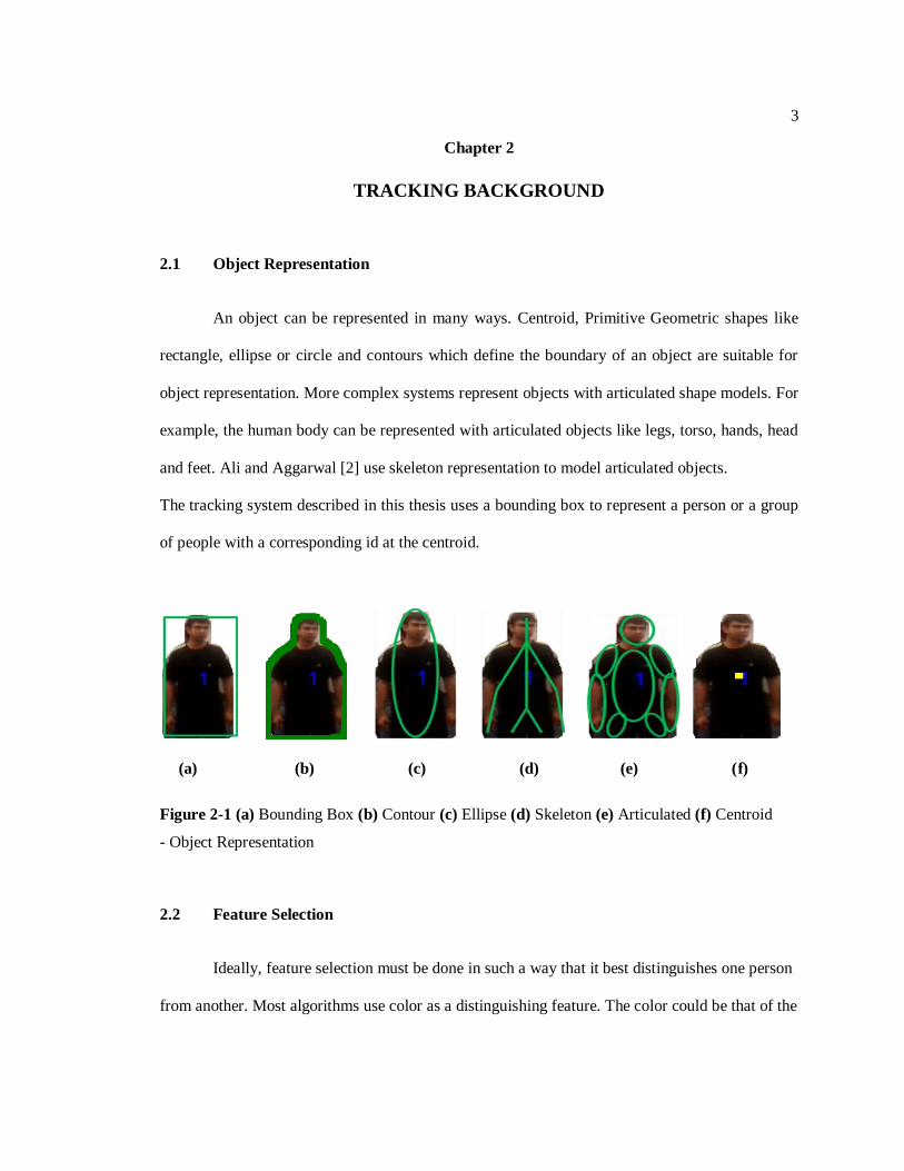
An object can be represented in many ways. Centroid, Primitive Geometric shapes like

rectangle, ellipse or circle and contours which define the boundary of an object are suitable for

object representation. More complex systems represent objects with articulated shape models. For

example, the human body can be represented with articulated objects like legs, torso, hands, head

and feet. Ali and Aggarwal [2] use skeleton representation to model articulated objects.

The tracking system described in this thesis uses a bounding box to represent a person or a group

of people with a corresponding id at the centroid.

(a) (b) (c) (d) (e) (f)

Figure 2-1 (a) Bounding Box (b) Contour (c) Ellipse (d) Skeleton (e) Articulated (f) Centroid

- Object Representation

2.2 Feature Selection

Ideally, feature selection must be done in such a way that it best distinguishes one person

from another. Most algorithms use color as a distinguishing feature. The color could be that of the

4

skin, or shirt or even a combination of both. In cases where illumination variation is large, color

might not be the best choice for distinguishing people. Optical flow methods are used for contour

tracking. Edges and texture are other features that have been used. Automatic feature selection

which dynamically utilizes a subset of features from a larger pool of features has gained great

popularity. The best feature is selected based on the weight assigned. In a pool with a large set of

features, one classifier can be trained for each feature. Adaboost is a popular algorithm that

selects the best classifier based on a set of weak classifiers. Color histograms are widely used to

quantify feature. The choice of the color space again depends on the requirement of the

application and scene.

In this thesis, a variant of color histogram is used for distinguishing people. It is called

the Integral Image which is the sum of the pixel intensities (8 bit gray scale values) within a

specified box in the image. More about this is explained in later chapters.

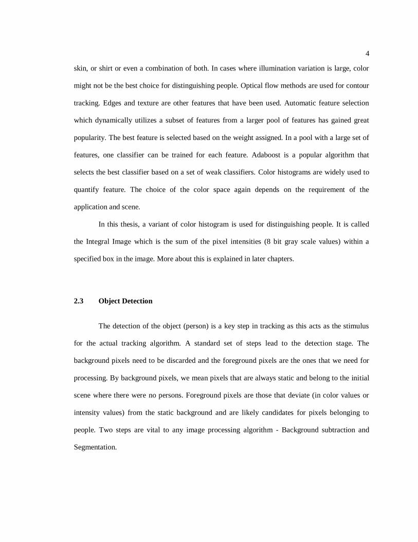
2.3 Object Detection

The detection of the object (person) is a key step in tracking as this acts as the stimulus

for the actual tracking algorithm. A standard set of steps lead to the detection stage. The

background pixels need to be discarded and the foreground pixels are the ones that we need for

processing. By background pixels, we mean pixels that are always static and belong to the initial

scene where there were no persons. Foreground pixels are those that deviate (in color values or

intensity values) from the static background and are likely candidates for pixels belonging to

people. Two steps are vital to any image processing algorithm - Background subtraction and

Segmentation.

5

2.3.1 Background Subtraction

As a first step, an average background image has to be stored and updated on a frame by

frame basis by the tracking system. This can be done by finding the average gray scale or RGB

value at each pixel location for a scene without any people in it. This can be called the training

period. In the process, the average RGB or 8-bit gray value of a pixel at (x, y) is found and at the

end of the training period a mean background image is obtained.

The first step in person detection is Background Subtraction, which extracts all the

foreground pixels in the current frame by comparing the value of the pixel at (x, y) in the current

frame with the value of the pixel at (x, y) in the background image. If the difference crosses a

threshold it is deemed a foreground pixel. If it lies within the threshold the new value is updated

in the background image in order to accommodate slight changes in intensities.

For indoor scenes, the threshold is usually selected by trial and run methods. Intensity

variation is assumed to be uniform across the frame and so a single threshold is good enough for

all the pixels in the frame. For outdoor scenes the threshold must be made adaptive and each pixel

has a different threshold. This is because there might be large variation of intensity at a particular

pixel due to non-static background (example. swaying trees). In Figure 2-2, the dark green pixels

represent background (denoted by 0) .The pixels which contain parts of the hand are labeled as

foreground (denoted by 1).

Figure 2-2 Background Subtraction

6

Appiah et.al have shown a single chip FPGA implementation of Background Subtraction

algorithm in [3].

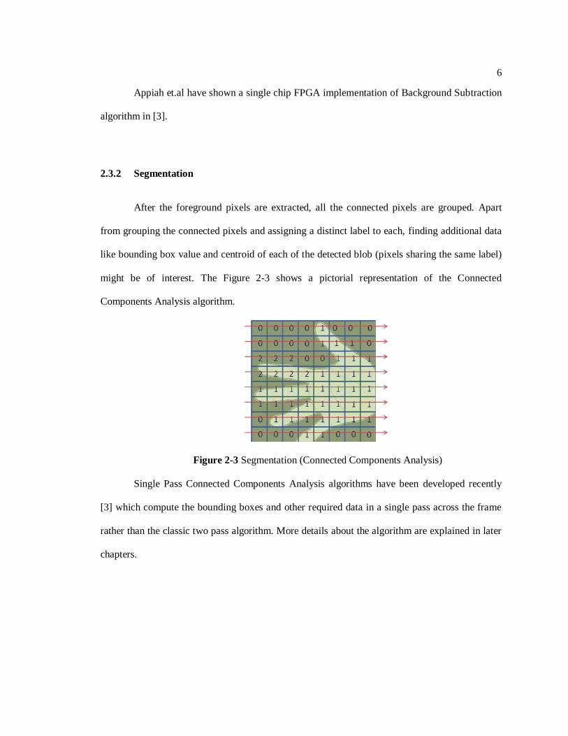
2.3.2 Segmentation

After the foreground pixels are extracted, all the connected pixels are grouped. Apart

from grouping the connected pixels and assigning a distinct label to each, finding additional data

like bounding box value and centroid of each of the detected blob (pixels sharing the same label)

might be of interest. The Figure 2-3 shows a pictorial representation of the Connected

Components Analysis algorithm.

Figure 2-3 Segmentation (Connected Components Analysis)

Single Pass Connected Components Analysis algorithms have been developed recently

[3] which compute the bounding boxes and other required data in a single pass across the frame

rather than the classic two pass algorithm. More details about the algorithm are explained in later

chapters.

7

2.3.3 Association

Once the required blobs are filtered, the next step is to associate each blob in the current

frame with a blob from the previous frame. This is a complex processing step as it might involve

merges and splits. By merges, we mean that a person might merge with another person partly or

completely. Again, after a few frames the same person might split from the merged blob. The

situation gets more complex if a group of people merge and the split randomly. Mean shift

tracking using centroid is a widely used algorithm to associate blobs in the current frame to

previous frame. This holds true because there is very small difference between the centroid

positions of a person in the current frame compared to his position in the previous frame.

Therefore, the centroid in the current frame that is closest to the centroid in the previous frame

can be thought of as the centroid of the same person. This might not be a complete solution as it

cannot handle cases of merges and splits.

Separate processing needs to be done to identify merges and splits. Once a person is

determined to be occluded with another person or a group of persons, we need to update only the

group behavior. The features of each separate individual have to be stored in memory. Assuming

that the merges and splits are identified, another association algorithm needs to be implemented

to match the split ids to the corresponding stored ids.

8

Chapter 3

BACKGROUND ESTIMATION

Background Estimation consists of two phases. In the first phase, which is the Training

phase, a set of N image frames without any humans in the scene, is sent to the Background

Estimation (BE) unit. The cumulative sum of the pixel values at each location is accumulated and

averaged to give a mean background image. This marks the end of the training phase. In the

second phase, which is the estimation phase, each incoming frame is differenced from the

background image at each pixel location and a threshold is applied on the difference value. If the

difference value is greater than this threshold, the pixel is recognized as foreground pixel and

represented by binary „1‟. If the difference value is less than the threshold, the pixel is represented

by binary „0‟ indicating it is a background pixel. Hence, at the end of the process, a binary image

is obtained with „1‟s representing the foreground regions in the current image and „0‟s

representing background regions in the current image.

3.1 Implementation

In our implementation we operate on grayscale images with each pixel represented by 8

bits. The current image, the background image and the binary image are all stored in DDR2

SDRAM memory.

9

3.1.1 Training Phase

The PowerPC controls the background subtraction unit by providing the required status

signals. Before beginning the training process, the Background Estimation Unit (BEU) is

configured with image size, starting addresses of current_pixel_memory and

average_pixel_memory and other required information, by the PowerPC. A start_training signal

is then issued by the PowerPC that makes the BEU to function in the training phase.

The arbiter services requests from the current_pixel_fifo (CPF), average_pixel_fifo

(APF) and the update_pixel_fifo (UPF). It is to be noted that during training, the

average_pixel_memory stores the sum of current pixels at each corresponding location, over N

frames. Therefore, a pixel location in average_pixel_memory is represented by 16 bits (assuming

sum of 8 bit pixels over a maximum of 256 training frames). Figure 3-1 gives the architecture of

the BEU in the training phase. As long as CPF and APF are not empty, pixels are read from CPF

and APF, added and stored in UPF. The CPF is read during alternate cycles to synchronize with

APF since the pixel width in CPF is 8 bits and pixel width in APF is 16 bits. The FIFO width of

the CPF and APF can be set to the data width of the PLB, to facilitate processing of multiple

pixels at a time. When the number of pixels in UPF crosses the threshold, a memory write is

requested. An interrupt signal is sent by the BEU to the PowerPC when end of frame is realized.

The number of training frames sent and processed by the BEU is kept track of by the PowerPC

and before issuing the start_average signal with the last training frame, the PowerPC configures

the BEU with the number of shift bits(to divide the total in APM with the number of training

frames) and asserts an average_flag signal. As shown in Figure 3-1 the pixels are added as usual

but before storing them in the UPF, a right shift is done by the amount of shift bits. It is to be

noted that the APM is updated with 8 bit value pixels during this phase. The update logic unit

takes care of writing the pixel values appropriately to average_pixel_memory.

10

Update Logic

Current

Pixel FIFOAverage Pixel

FIFOUpdate Pixel

FIFO

+

+

+

+

+

+

Average

FlagShift No Shift

ARBITER

CURRENT PIXEL

MEMORY

AVERAGE PIXEL

MEMORY

DDR2 SDRAM

RGB to GRAY

Converter

Figure 3-1 Hardware Implementation of Training Phase in Background Subtraction

11

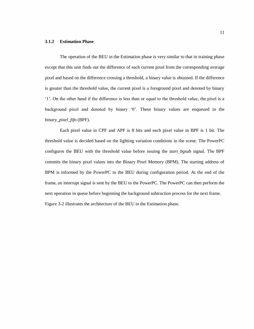
3.1.2 Estimation Phase

The operation of the BEU in the Estimation phase is very similar to that in training phase

except that this unit finds out the difference of each current pixel from the corresponding average

pixel and based on the difference crossing a threshold, a binary value is obtained. If the difference

is greater than the threshold value, the current pixel is a foreground pixel and denoted by binary

„1‟. On the other hand if the difference is less than or equal to the threshold value, the pixel is a

background pixel and denoted by binary „0‟. These binary values are enqueued in the

binary_pixel_fifo (BPF).

Each pixel value in CPF and APF is 8 bits and each pixel value in BPF is 1 bit. The

threshold value is decided based on the lighting variation conditions in the scene. The PowerPC

configures the BEU with the threshold value before issuing the start_bgsub signal. The BPF

commits the binary pixel values into the Binary Pixel Memory (BPM). The starting address of

BPM is informed by the PowerPC to the BEU during configuration period. At the end of the

frame, an interrupt signal is sent by the BEU to the PowerPC. The PowerPC can then perform the

next operation in queue before beginning the background subtraction process for the next frame.

Figure 3-2 illustrates the architecture of the BEU in the Estimation phase.

12

Figure 3-2 Hardware Implementation of Estimation Phase in Background Subtraction

13

Figure 3-3: Background Subtraction Illustration

Background Frame (top); Current Frame (middle); Background Subtraction (bottom)

14

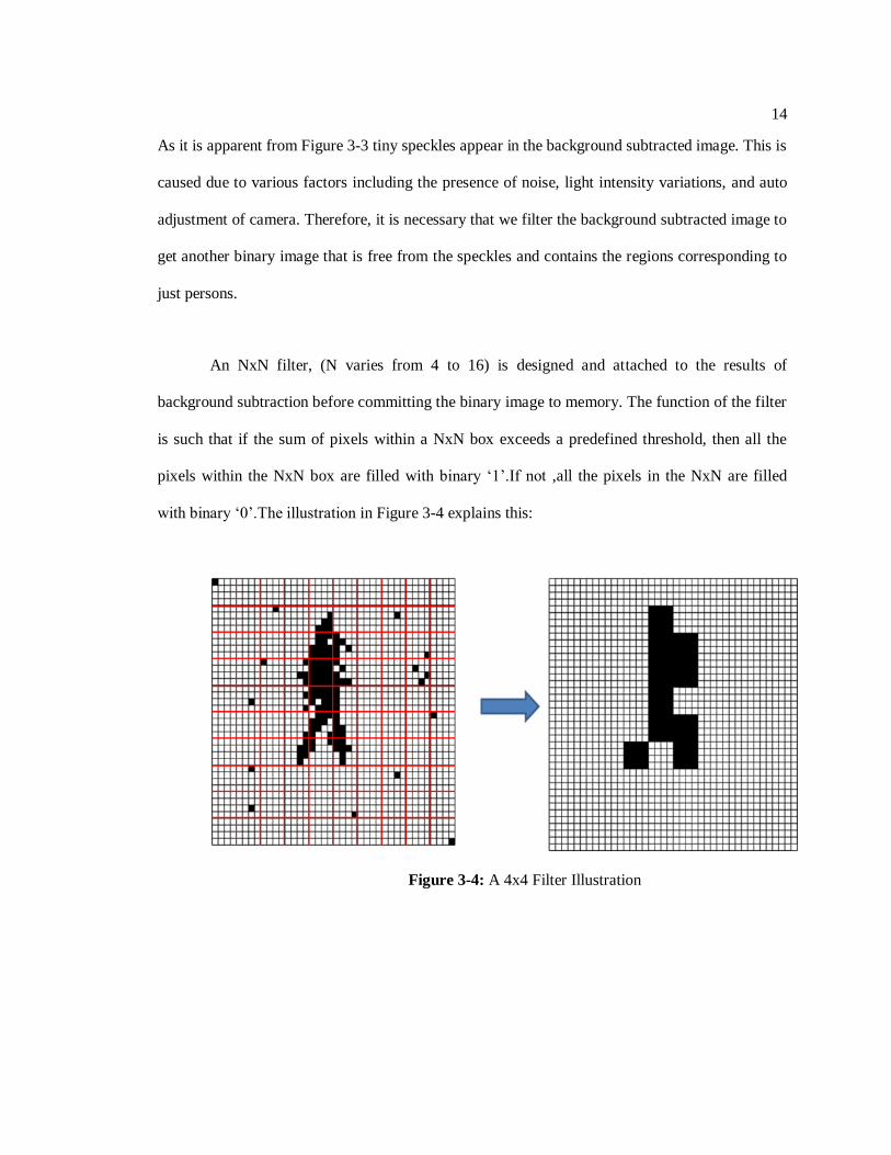
As it is apparent from Figure 3-3 tiny speckles appear in the background subtracted image. This is

caused due to various factors including the presence of noise, light intensity variations, and auto

adjustment of camera. Therefore, it is necessary that we filter the background subtracted image to

get another binary image that is free from the speckles and contains the regions corresponding to

just persons.

An NxN filter, (N varies from 4 to 16) is designed and attached to the results of

background subtraction before committing the binary image to memory. The function of the filter

is such that if the sum of pixels within a NxN box exceeds a predefined threshold, then all the

pixels within the NxN box are filled with binary „1‟.If not ,all the pixels in the NxN are filled

with binary „0‟.The illustration in Figure 3-4 explains this:

Figure 3-4: A 4x4 Filter Illustration

15

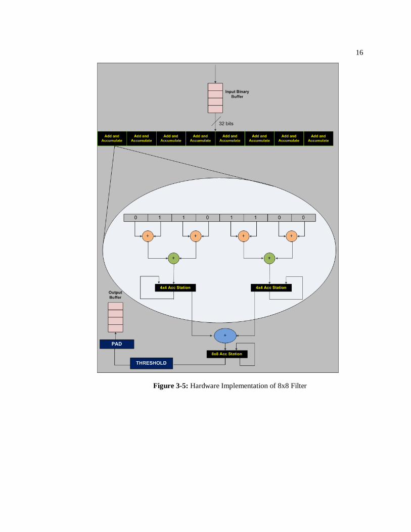
3.1.3 Hardware Implementation

The NxN filter is designed with a 4x4 granularity. The results from the background

subtraction unit are streamed into an Input Binary Buffer that is 32 bits wide. As data is read from

the Input Binary Buffer, the sum of every four consecutive bits is found in a pipelined fashion and

stored in a 4x4 accumulation station. When the next row is being processed, the sum of every 4

pixels is added to the sum of the 4 pixels above (stored in the 4x4 accumulation station).When the

row count reaches four, the 4x4 sum is ready. Based on the size of the filter, the result can be sent

to a threshold unit or sent for further processing. If the filter is a 4x4 filter the result is compared

with a threshold. If the sum exceeds the threshold, then all the 4x4 pixels are transformed to

binary 1‟s.If not, the 4x4 box is all binary „0‟s.

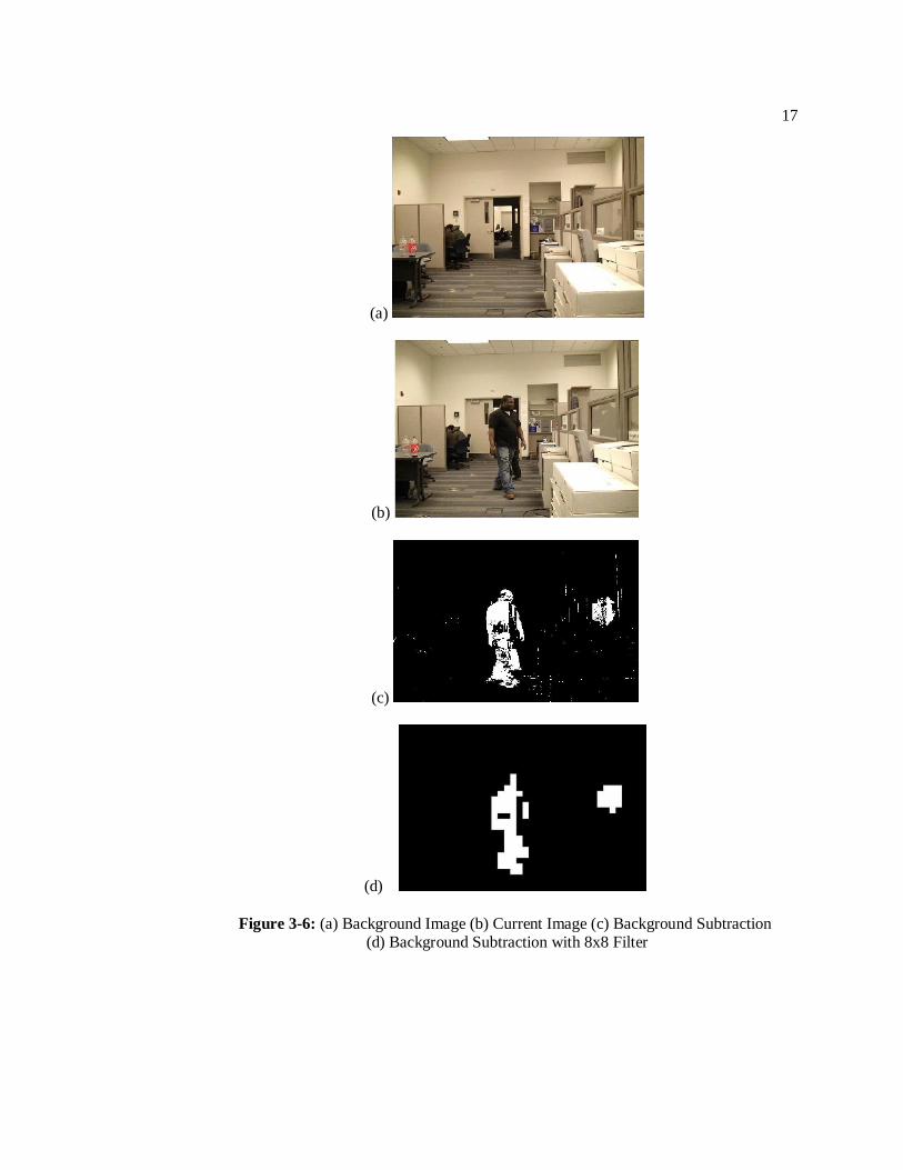
If the required filter is an 8x8 filter, then the 4x4 sum is sent to an 8x8 accumulation

station where a similar summing process is repeated. When the 8x8 sum is ready, it is sent to the

threshold unit and padded accordingly. In our implementation we use an 8x8 filter for obtaining

best results. Figure 3-5 shows the hardware implementation of the 8x8 Filter block and Figure 3-6

illustrates the results after the filter is applied to the output from the Background Estimation Unit.

16

Figure 3-5: Hardware Implementation of 8x8 Filter

17

(a)

(b)

(c)

(d)

Figure 3-6: (a) Background Image (b) Current Image (c) Background Subtraction (d) Background Subtraction with 8x8 Filter

18

Chapter 4

CONNECTED COMPONENT LABELING

Given an MxN binary image, Connected Component Labeling (CCL) assigns a unique

label to each disjoint pixel region in the image. A disjoint pixel region is an image patch in which

each foreground pixel has zero or more adjacent foreground pixels. This is useful in many

applications that require segmentation of connected foreground pixels before subsequent

processing of those regions can commence. Apart from assigning a unique label, CCL can be

enhanced to extract more useful data from connected regions. Examples of such ancillary

information include bounding box coordinates, centroid coordinates, and connected region area.

An example use of this algorithm is in human pedestrian tracking. First, a background

segmentation process distinguishes pixels belonging to a static background and those belonging

to objects in the foreground, giving them values binary „0‟ and „1‟ respectively. By applying CCL

to the resulting bitmap, the bounding boxes of all disjoint regions are determined. If the

dimensions of a bounding box are consistent with the width and height ratios of human

pedestrians, the region can be considered to represent a pedestrian.

For reasons to become apparent in the following discussions, FPGAs have particular

advantage over competing technologies in offering high-performance implementation of the

Connected Component Labeling algorithm. Bit-level granularity of access and manipulation is

best suited to fine grain FPGA fabrics. Moreover, the ability to implement complex, single-cycle

control structures makes FPGAs the optimal choice for control-intensive CCL implementations.

19

4.1 Related Work

The first parallel hardware implementation of Connected Component Labeling was

described by Ranganathan et. al [4]. The design was based on a two pass algorithm capable of

processing a single 128x128 image in 900 microseconds: well above real time constraints. The

advantages of raster scan based image segmentation are discussed in [5]. Several high speed

parallel but resource intensive algorithms are discussed in [6]. A resource efficient iterative

algorithm implemented on FPGA is discussed in [7] but requires an indeterminate number of

passes as highlighted in [8]. Bailey et.al developed a single pass labeling algorithm [8] amenable

to a streaming architecture implementation. Their FPGA implementation, discussed in [9]

requires minimal storage as each input pixel is comprehensively processed as they arrive

sequentially from the video source. The main drawback of the architecture is the limitation of the

pipeline to process more than a single pixel per cycle. This constrains the possible input

modalities that can directly interface with the pipeline. Moreover, the architecture relies on the

presence of video blanking periods to perform costly merge operations at the end of each row.

While video blanking periods are common to most CCD and CMOS camera interfaces, they do

not exist when interfacing directly to a memory subsystem for which data can be accessed back-

to-back with negligible delay. This work enhances the single pass algorithm allowing its use in

systems requiring more diverse pixel input rates, interfaces, and protocols.

4.2 Single Pass Algorithm

To label a pixel, we consider its four connected neighbors as shown in Figure 4-1 and observe

the following:

20

2 2 2

2 ?

2 2 2

2 0

No Labeling

0 0 0

0 ?

0 0 0

0 2

New Labeling

2 0 3

2 ?

2 0 2

2 2

Merging

6 0 0

0 ?

6 0 0

0 6

Inherited

Labeling

(a)

(b)

(c)

(d)

‘x’ Foreground Pixel with Label ‘x’

? Current Foreground Pixel ? Current Background Pixel

0 Background Pixel

Legend

Figure 4-1: Pixel Labeling

As shown in Figure 4-2 the neighboring pixel labels are stored in fast, zero-latency, registers

L, UL, U, and UR corresponding to the Left, Upper Left, Upper, and Upper Right locations

respectively. The labels from the previous row are cached in a buffer that exhibits a single cycle

a) IF the current pixel is a background pixel THEN it is given label „0‟.

b) IF all neighboring pixels are background AND the current pixel is a foreground pixel

THEN a new label is assigned.

c) IF only a single label is used among the labeled neighbors AND the current pixel is a

foreground pixel THEN the current pixel inherits that label.

d) IF differing labels are used among the neighbors AND the current pixel is a foreground

pixel THEN the current pixel will merge the labeled regions and the current pixel and all

labeled pixels will be labeled with the smallest label in the neighborhood

21

penalty during read and write access. This fact requires particular attention when considering the

Merging Scenario (Figure 4-1.d). As the example shows, all existing references to label „3‟ in the

row buffer should reference label „2‟ once the merge completes. Rather than search the entire

row buffer replacing all occurrences of the label „3‟ with label „2‟, a practical implementation

uses a lookup table to store and retrieve aliases for a given label. This Merge Table is indexed by

a label, Lreference, and returns the actual label, Lactual, for which Lreference has merged with since the

row buffer was initialized.

4.2.1 Pixel Buffer

The input to CCL is a binary image representing the background (0) or foreground (1)

classification of an image. In a byte accessible memory a single byte represents the state of eight

pixels. If a byte is fetched per cycle, it would take eight subsequent cycles for the CCL pipeline to

process each pixel. More realistically, in a system with a 64-bit system bus supporting a 16 cycle

burst transactions, 1024 (64x16) status bits can be delivered in a single transaction. For discussion

sake, we refer to this unit of transfer a Fetch Line. Consequently, the memory subsystem would

remain idle for 1024-16 cycles before being tasked to supply an additional Fetch Line. If no other

memory requests are pending much of the memory subsystem‟s bandwidth would be unused.

The lexicographic dependency of pixels in the labeling process makes it impractical to label

more than two sequential pixels at a time. Instead we extract parallelism by partitioning the image

frame and performing SCCL independently and simultaneously on each partition. In a final step

we combine the results of each independent labeling process to produce the complete image

labeling.

22

A C CtB

LABEL PROCESSING

D

PIXEL BUFFER

ROW BUFFER

MERGE TABLE

ROW,COL

COUNT

END OF ROW RESOLVE

MERGE

BOUNDING BOX

DATA TABLE

END OF BOX

CALCULATION

VALID

BB_FIFO

BINARY IMAGE FROM

MAIN MEMORY

BOUNDING BOX

Current Pixel

Figure 4-2: Streaming Single Pass Architecture

4.2.2 End of Box Detection

In our implementation we determine the bounding boxes as we process the pixel stream

and forward the coordinates as soon as they are known. To facilitate this we employ two tables:

The Bounding Box Coordinate Table, BBCT, and the Bounding Box Coordinate Cache, BBCC,

both implemented as dual port RAMs. The BBCC stores the maximum column coordinate of a

label in the current row. The BBCC is written at address D when the current pixel is a

background pixel and the previous was a foreground pixel. (D!=0,current_pixel=0) .The BBCC is

read at address A when the pattern (current pixel = 0, A!=0, B = 0 and D = 0) is detected. This

pattern indicates that the pixel at location A is the lower rightmost pixel in the region containing

A. The pattern enables a state machine that reads the BBCC location corresponding to label A

and the BBCT location corresponding to label A. The current column coordinate is compared

23

with the output from the BBCC and the current row coordinate is compared with the maximum

row value of the label A from the BBCT output.

00

0A

3 3 3 3 3 1 1 1 1 1

3 3 3 3 3 3 3 1 1 1 1 1 1 1 1 1

0

0 0 0000 0 0 0 0 0

00 000000000000000

4 4

0

1

2

0 1 2

0 1 2 3 4 5 6 7 8 9 10 11 12 13 14 15 16 17 18

012

COLUMN COORDINATE

RO

W C

OO

RD

INA

TE

X

10,18,0,0

X

0,7,0,0

X

0

1

2

3

4

X

9,18,0,1

X

0,7,0,1

X

0

1

2

3

4

X

9,18,0,1

X

0,7,0,1

17,18,2,2

0

1

2

3

4

X

13

X

5

18

0

1

2

3

4

X

13

X

5

X

0

1

2

3

4

X

18

X

7

X

0

1

2

3

4

Bounding Box

Coordinate Table

Bounding Box

Coordinate

Cache

Figure 4-3: End of Bounding Box Detection

If the current column and row are both greater than the corresponding pair of outputs

from the two tables, then it is the end of the bounding box with label A. This is illustrated in the

Figure 4-3.

When processing row 0, the BBCT records the {min_x, max_x, min_y, max_y}

coordinates of labels 3 and 1 as {0, 7, 0, 0} and {10, 18, 0, 0} respectively. The BBCC records

the column coordinates 18 and 7 for labels 3 and 1 respectively which are the maximum of these

labels in row 0. At column 8 in row 1, the pattern 3,0,0,0 is detected and the coordinates

corresponding to label 3 in both tables are retrieved. The BBCC table returns 5 which is the last

updated column coordinate and the BBCT returns a maximum row coordinate of 1 which is equal

to the current row.

24

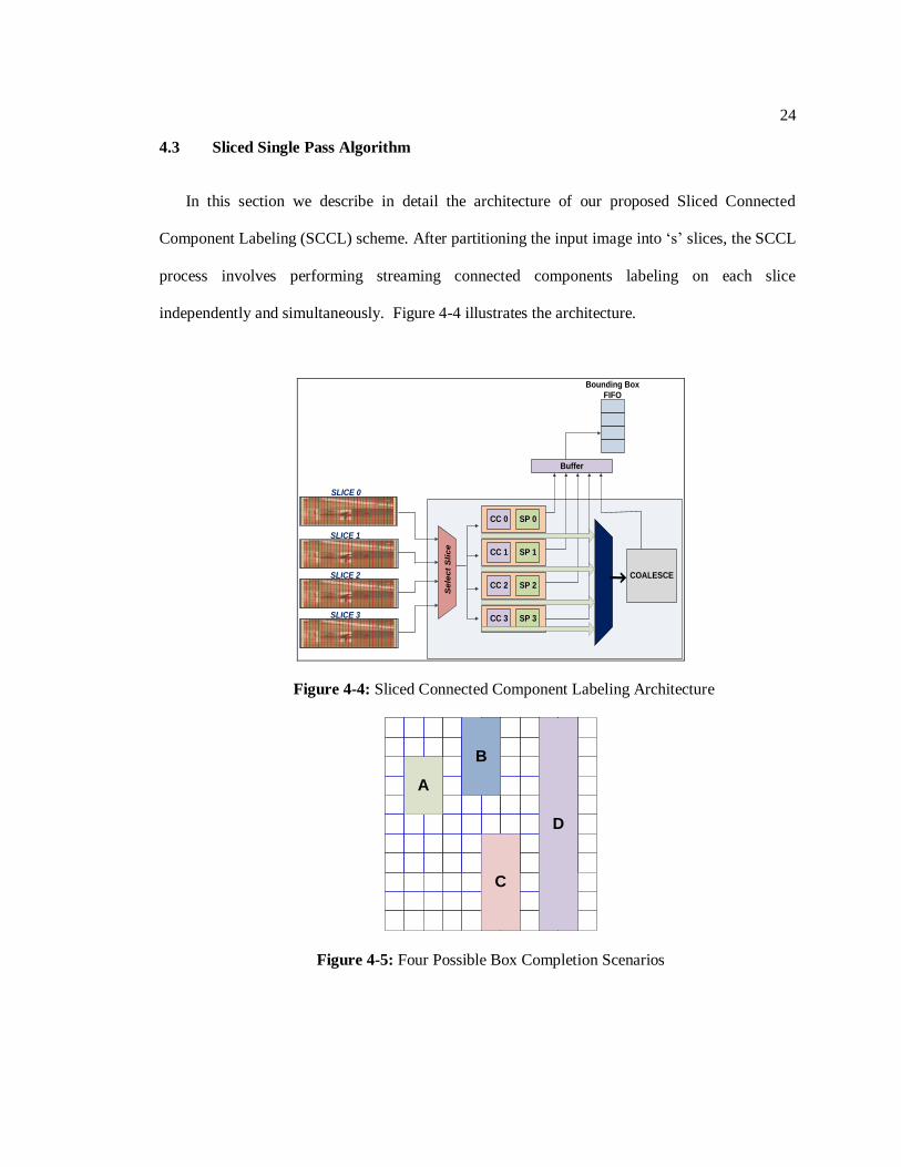
4.3 Sliced Single Pass Algorithm

In this section we describe in detail the architecture of our proposed Sliced Connected

Component Labeling (SCCL) scheme. After partitioning the input image into „s‟ slices, the SCCL

process involves performing streaming connected components labeling on each slice

independently and simultaneously. Figure 4-4 illustrates the architecture.

CC 3 SP 3

CC 2 SP 2

CC 1 SP 1

CC 0 SP 0

Se

lec

t S

lic

e

Buffer

Bounding Box

FIFO

COALESCE

SLICE 0

SLICE 1

SLICE 2

SLICE 3

Figure 4-4: Sliced Connected Component Labeling Architecture

A

B

C

D

Figure 4-5: Four Possible Box Completion Scenarios

25

4.3.1 Algorithm Motivation and Overview

The four possible scenarios in which a box may finish within a slice are highlighted in

Figure 4-5. Note that each box highlights the limits of a label and not the actual shape of the

label. Each CCL detects the end of a box and forwards its label for appropriate processing. The

Box labeled A needs no further processing because its top and bottom limits do not lie on the top

or bottom boundary of the slice. Contrarily, the labels of the other three boxes viz. B,C and D are

saved for further processing to determine if they coalesce with any other boxes in the adjacent top

or bottom slices. To determine the connection, if any, between labels from two adjoining slices,

we must establish an association between the labels from the last row of the top slice and the the

top row of the bottom slice. Within each slice we employ a buffer to store the label assigned to

each pixel while processing the first row. Note that at the end of CCL processing the labels may

differ from those assigned at start due to merging. In Figure 4-5, if labels B and D merged at

some point then label D would be invalid, however the first row buffer would still reference D.

Consequently, extra processing is required to monitor the labels assigned in the first row.

Coalescing is performed in two phases: In the first phase the association between labels

lying at the bottom boundary of slice n and the top boundary of slice n+1 are recorded. In the

second phase the recorded associates are resolved. This is done by reading the association queue

and detecting boxes that do not continue beyond the current slice and committing them or

updating a Global Bounding Box table for labels that continue to stretch across slices. This

process is repeated for all slice boundaries until all boxes are committed.

26

4.3.2 Connected Component Processor

As shown in figure 4-4, each Connected Component Processor, CCP, handles a slice that

is composed of a range of rows. Consider an input image of size 240x320 that is split into 8

slices. Then, rows 0 to 29 are handled by CCP0, rows 30 to 59 by CCP1, and so on up to CCP7

which will handle rows 210 to 239.

Reading Rows: Each Connected Component Processor, CCP, accesses memory to fetch rows for

its associated slice. As discussed in section x, pixels can be fetched at a much higher rate than

they can be processed. We leverage this disparity to service the fetch requests of multiple CCPs

in parallel. Following our example, CCP0 fetches row 0 and starts processing. Once CCP0 is done

fetching row 0 and while it is processing, CCP1 starts fetching and processing row 30. Similarly,

other CCPs will fetch and process the first row of their dedicated slices. In this way, the

architecture processes a row in each slice in parallel. When CCP7 is done fetching row 210, its

first row, memory access is granted to CCP0 which fetches and processes row 1, its second row.

This process continues until all the CCPs have fully processed the range of rows in its dedicated

slice.

4.3.3 Slice Processor

The Slice Processor (SP) determines the remaining processing required for each box

region completed within a slice. Either the coordinates of the region are committed to the output

queue or retained locally for further processing in the coalescing stage. When a CCP detects the

end of a bounding box, it will send the box coordinates to the corresponding SP. The SP checks if

the box boundary lies on the top or bottom of the slice by analyzing the minimum and maximum

row coordinates respectively. If the box does not intersect ether slice boundary, the box

27

coordinates are enqueued into the Output Queue indicating that the box requires no further

processing. Alternatively, if the box intersects either the top or bottom slice boundary the SP will

place the box coordinates and label in the Coalesce Queue, indicating that further processing is

required in the coalescing stage. The SP maintains a record of labels assigned in the top row of its

slice. This is necessary because the labels assigned in the top row may merge amongst themselves

and result in different labelings as box extents are detected. Therefore, additional record keeping

as highlighted in Figure 4-7 is required.

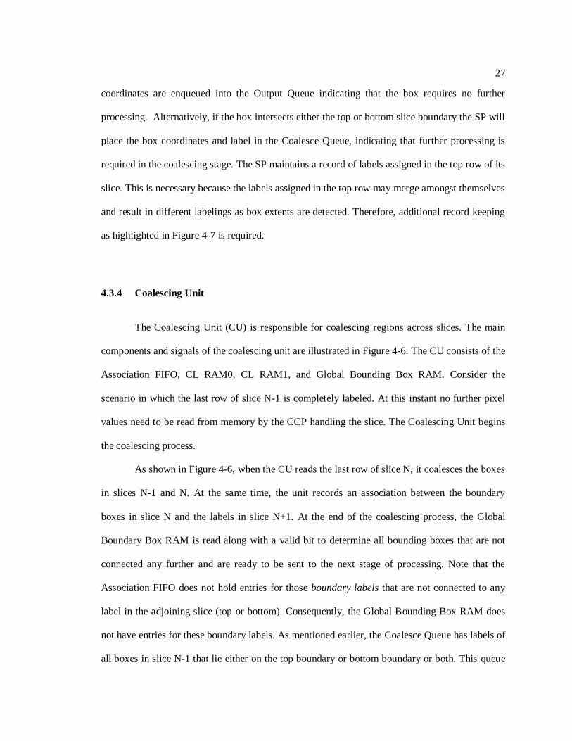
4.3.4 Coalescing Unit

The Coalescing Unit (CU) is responsible for coalescing regions across slices. The main

components and signals of the coalescing unit are illustrated in Figure 4-6. The CU consists of the

Association FIFO, CL RAM0, CL RAM1, and Global Bounding Box RAM. Consider the

scenario in which the last row of slice N-1 is completely labeled. At this instant no further pixel

values need to be read from memory by the CCP handling the slice. The Coalescing Unit begins

the coalescing process.

As shown in Figure 4-6, when the CU reads the last row of slice N, it coalesces the boxes

in slices N-1 and N. At the same time, the unit records an association between the boundary

boxes in slice N and the labels in slice N+1. At the end of the coalescing process, the Global

Boundary Box RAM is read along with a valid bit to determine all bounding boxes that are not

connected any further and are ready to be sent to the next stage of processing. Note that the

Association FIFO does not hold entries for those boundary labels that are not connected to any

label in the adjoining slice (top or bottom). Consequently, the Global Bounding Box RAM does

not have entries for these boundary labels. As mentioned earlier, the Coalesce Queue has labels of

all boxes in slice N-1 that lie either on the top boundary or bottom boundary or both. This queue

28

is read one by one and a connectivity check is done as explained later to find out if the labels are

connected at the top or bottom. If they are unconnected at both ends, the labels are ready for

commit.

Figure 4-6: Coalescing Unit Architecture

4.3.5 Functions of the Slice Processor

Function 1: Monitor the labels assigned in the first row in the dedicated range of rows

and keep a count.

01 2 3 4

0 0 0

11 2 3 4

0 0 0New label ‘1’

11 2 3 4

1 0 0New label ‘2’

0

COUNT

11 2 3 4

01 1

1

2

3New label ‘3’

Initial Condition

29

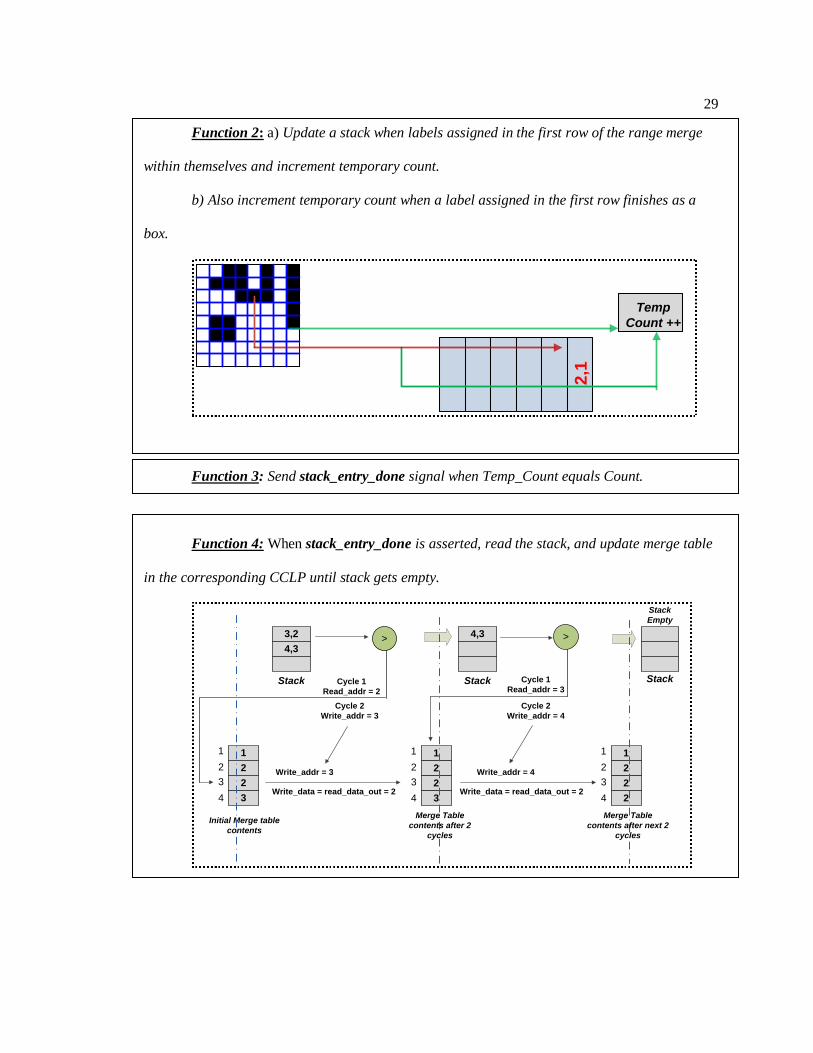
Function 2: a) Update a stack when labels assigned in the first row of the range merge

within themselves and increment temporary count.

b) Also increment temporary count when a label assigned in the first row finishes as a

box.

Temp

Count ++

2,1

Function 3: Send stack_entry_done signal when Temp_Count equals Count.

Function 4: When stack_entry_done is asserted, read the stack, and update merge table

in the corresponding CCLP until stack gets empty.

3,2

4,3>

11

2

3

4

2

2

3

Stack

Initial Merge table

contents

Cycle 1

Read_addr = 2

Cycle 2

Write_addr = 3

Write_addr = 3

Write_data = read_data_out = 2

11

2

3

4

2

2

3

4,3

Stack

>

Cycle 1

Read_addr = 3

Cycle 2

Write_addr = 4

11

2

3

4

2

2

2

Write_addr = 4

Write_data = read_data_out = 2

Stack

Stack

Empty

Merge Table

contents after 2

cycles

Merge Table

contents after next 2

cycles

30

Function 5: When end_of_box signal is asserted, redirect the box labels to appropriate

FIFOs

End_of_box_valid

Box Label

Box Data

AB

C

D

Coalesce Queue

Output Queue

Figure 4-7: Slice Processor Functionalities

4.3.6 Enqueueing the Association FIFO

The Coalescing Unit needs to establish an association between slices N-1 and N. The SP

that handles slice N stores the first row labels in a buffer as mentioned earlier. The labels of the

last row of slice N-1 are already stored in the row buffer of the CCP handling that particular slice

and the Merge Table of this CCP has the updated values of these labels. The values from the first

row of slice N are read from the first row buffer, whereas the values from the last row buffer of

slice N-1 are read from the Merge Table – indexed by the value from the last row buffer as

discussed earlier – in order to obtain the updated values. The two values that are read are checked

and written as {top_label,bottom_label} to an Association FIFO as shown in Figure 4-8. In order

to avoid redundant writes, the previous write value is cached and this cached value is compared

with the current value before writing.

31

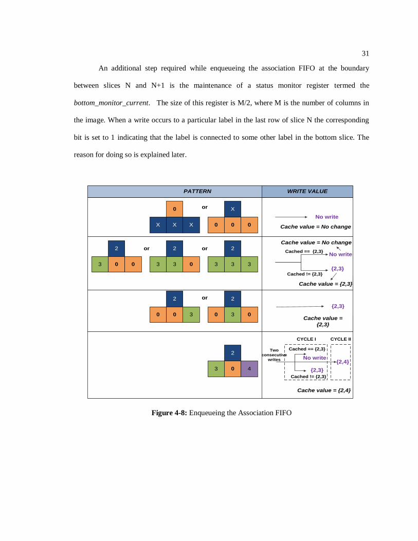
An additional step required while enqueueing the association FIFO at the boundary

between slices N and N+1 is the maintenance of a status monitor register termed the

bottom_monitor_current. The size of this register is M/2, where M is the number of columns in

the image. When a write occurs to a particular label in the last row of slice N the corresponding

bit is set to 1 indicating that the label is connected to some other label in the bottom slice. The

reason for doing so is explained later.

X

0

XX

No write

0 00

X

2

3 3 3

Cached == {2,3}

Cached != {2,3}

No write

{2,3}

2

0 3 0

2

0 30

or

2

3 03

2

03 0

oror

{2,3}

2

03 4

Two

consecutive

writes

Cached == {2,3}

Cached != {2,3}

No write

{2,3}

CYCLE I CYCLE II

{2,4}

WRITE VALUEPATTERN

or

Cache value = No change

Cache value = {2,3}

Cache value = No change

Cache value =

{2,3}

Cache value = {2,4}

Figure 4-8: Enqueueing the Association FIFO

32

4.3.7 Dequeueing the Association FIFO

The actual coalescing of slice N-1 and slice N is done when the last row of slice N is

being read. Therefore, dequeueing the Association FIFO between slice N-1 and slice N and

enqueueing the Association FIFO between slice N and slice N+1 might occur simultaneously.

The reading starts once the stack corresponding to slice N discussed in the previous subsection

becomes empty. A counter is needed to store the number of previous writes based on which of the

association values are read. This is because a single FIFO is used to carry out the association

between slices in order. The value read from the association FIFO is of the form {A0, A1} where

A0 is an updated label from the last row of slice N-1, whereas A1 is a stale label from the first

row of slice N. The updated values of the first row labels of slice N are stored in the merger table

as discussed earlier. Therefore, indexing the merger table with A1 would return the updated value

of A1. Let us call the returned value A1‟. To meet cycle requirements, A0 has to be registered.

Let us also call the registered A0 as A0‟. Status registers called entry registers are maintained to

track connectivity. One M/2 bit register for the upper slice (slice N-1) termed

upper_entry_register and one M/2 bit register for the bottom slice (slice N) termed

bottom_entry_register. Note that the entry registers are updated during the read phase of the

Association FIFO and the bottom_monitor_current register is updated during the write phase of

the Association FIFO.

Figure 4-9 and Table 4-1 illustrate the update process done at the boundary between two slices.

33

Figure 4-9: Updating Association FIFO Example

Table 4-1 Updating Association FIFO Example

Time Instant Write Value Cache Labels Comments

0 and 1 None 0 2 {3,1} {3,1}

3,4 and 5 None {3,1} Cache value is same as write value

6 {2,1} {2,1} Cache value is different

7,8,9 and10 None {2,1}

11 {3,2} {3,2}

12 and 13 None {3,2}

14 None {3,2} Merge occurs (two consecutive

writes)

15 {3,3} {3,3} Second write (Note that A>=0 in

the next cycle does not matter)

16 {6,3} {6,3}

17 None {6,3}

18 None 0 Reset cache label to 0(last column)

34

4.3.8 Common Label (CL) RAMs

There are two CL RAMs; Upper and lower. These CL RAMs store a common reference

label – starting from decimal 1 – for the connected labels between any two slices. The entry

registers for A0‟ and A1‟ are retrieved and the subsequent processing is determined by the

following

Note. After processing every boundary, the two CL RAMs are switched. The entry registers of

the current upper CL RAM are zeroed (current upper_entry_register = 0) and becomes the lower

CL RAM while coalescing slices N and N+1.The current lower CL RAM becomes the next upper

CL RAM but its entry registers (current upper_entry_register = previous bottom_entry_register)

are kept as it is, to maintain the connectivity history.

1) If both are 0, then a new common label is written both in the upper CL RAM

indexed by A0‟ and lower CL RAM indexed by A1‟. Also, the new common label

value is incremented, while the entry registers corresponding to these labels are set

to 1.

2) If entry register corresponding to A0‟ is 0 and entry register corresponding to A1‟ is 1, then this means that the label A1‟ in the bottom slice is already connected to some

other label in the top slice, however, the label A0‟ in the upper slice is not connected

to any other label in the bottom slice. Therefore, the corresponding entry registers

are validated and the common label value output indexed by A1‟ in the lower CL

RAM is written into the upper CL RAM indexed by A0‟.

3) If entry register corresponding to A0‟ is 1 and entry register corresponding to A1‟ is

0 then it means the label A0‟ in the upper slice is already connected to some other

label in the bottom slice but the label A1‟ in the bottom slice is not connected to any

other label in the top slice yet. So the corresponding entry registers are validated and

the common label value output indexed by A0‟ in the upper CL RAM is written into

the lower CL RAM indexed by A1‟.

4) If both entry registers are 1 then it means both the labels A0‟ and A1‟ are already connected to some other label(s) in the bottom slice and top slice respectively. A

comparison of the output common labels from both CL RAMS is made to ensure

they are the same. If they are not the same, then the lower common label has to

replace the higher common label. If not, no update is needed.

35

4.3.9 Updating Global Bounding Box RAM

The Global Bounding Box RAM stores the Bounding box values of the common labels.

While reading the CL RAMs, the Bounding Box data tables from the CCs are also read. A0‟ is

used to read the BB of the upper slice and A1‟ is used to read the BB of the lower slice. The 2 bit

entry as mentioned in the previous section is registered, and in the next cycle, the Global

Bounding Box RAM is read with the common label as index. Based on the registered 2 bit value

the update of the Global Bounding Box RAM takes place.

4.3.10 Bounding Box Update

At the end of coalescing, we have an updated Global Bounding Box RAM with a

validity bit for each label either set or reset. Before reading the contents of the Global Bounding

Box Ram, the Coalesce Queue is read until empty. If the id read from the queue is unconnected

both at the top AND the bottom(which can be obtained from the corresponding entry register and

bottom_monitor_current register), it is committed immediately by fetching the value from the

corresponding bounding box table in CC. If not the entry is just discarded. This is repeated until

1) If both the values are 0 it means there is no entry for the new common label. So the two

BB values from the CC are compared and the updated BB is found. With the new common

label as index, the value is written to BB. When a new common label is assigned, a box

counter is incremented to keep track of the number of boxes that have coalesced.

2) If 01, then the values to be compared are the BB from top slice CC and the BB from

global BB ram. The final BB is found and with the common label as index the Global BB

ram is updated.

3) If 10, the values to be compared are BB from bottom slice CC and BB from global BB ram. The final BB is found and with the common label as index the Global BB ram is

updated.

4) If 11, and the common labels are different, then both the values are read form global ram

and the smaller of the two labels is updated with the final BB. A valid bit has to be set for

the higher label, which indicates it is not a valid label anymore. Also the box counter has to

be decremented.

36

the queue becomes empty. At the end of Coalescing the Global Bounding Box RAM is read

along with a validity bit till the count reaches the global id count and the boxes are committed to

the output buffer. When end of box count is reached we reset the registers in coalesce block and

send a coalesce end signal.

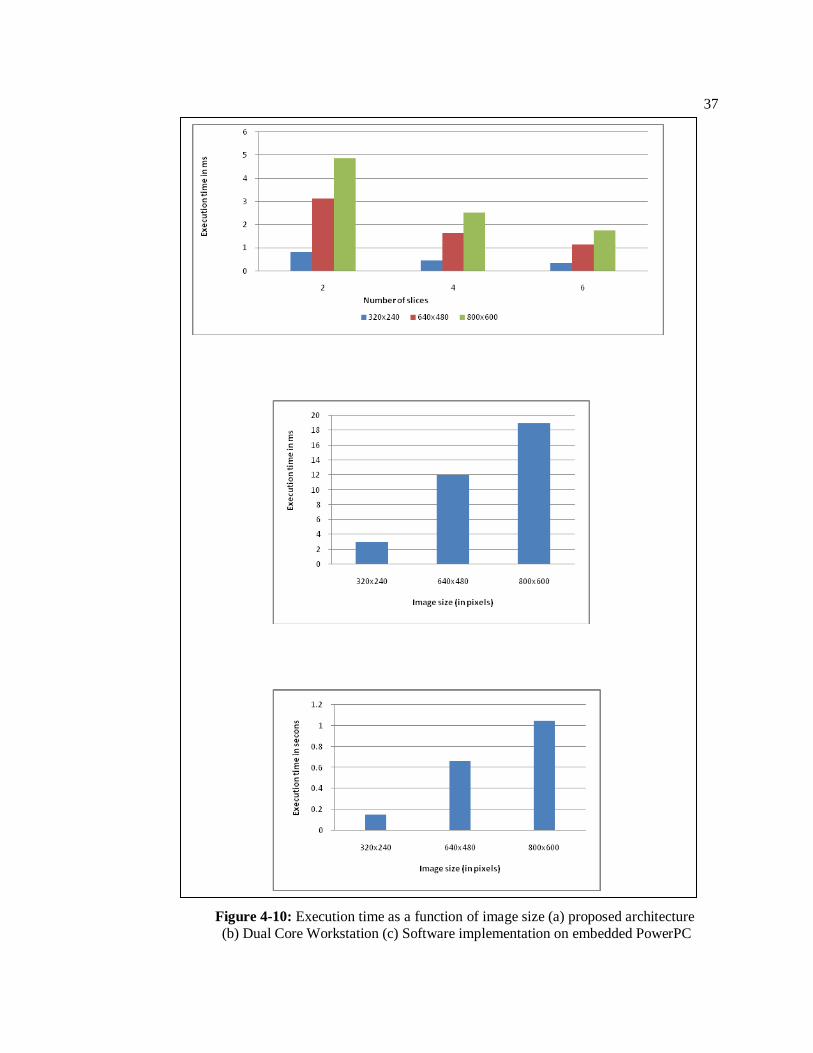
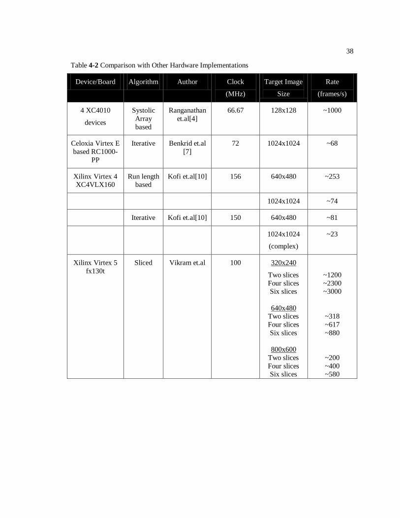
4.3.11 Results

A verilog implementation of the Connected Component Labeling architecture was simulated

using ModelSim mixed-language simulation environment and validated on a Xilinx Virtex-5

FPGA development platform. The ML510 development board is based on a Virtex-5 FX130T

FPGA which includes a PowerPC processor. The performance results are shown in Figure 4-10.

We compare our hardware implementation for varying image sizes and number of Slice

Processors. As a reference we have implemented a multi-pass version in C# executing on a 3.18

GHz Dual Core Xeon workstation as well as on the embedded PowerPC in the FPGA fabric. Our

architecture running at 100MHz outperforms the PowerPC reference implementation running at

300 MHz by a factor of approximately 215 and the workstation by a factor of 4. Note that our

hardware results account for the bandwidth and latency characteristics of a realistic embedded

system accessing a DDR2 memory device. In addition, the results show that our architecture

scales favorably with the input image size as additional slice processors can be added as

necessary. Also, a comparison with other previous hardware implementations is illustrated in

Table 4-2.

37

Figure 4-10: Execution time as a function of image size (a) proposed architecture

(b) Dual Core Workstation (c) Software implementation on embedded PowerPC

38

Table 4-2 Comparison with Other Hardware Implementations

Device/Board Algorithm Author Clock

(MHz)

Target Image

Size

Rate

(frames/s)

4 XC4010

devices

Systolic

Array

based

Ranganathan

et.al[4]

66.67 128x128 ~1000

Celoxia Virtex E

based RC1000-

PP

Iterative Benkrid et.al

[7]

72 1024x1024 ~68

Xilinx Virtex 4 XC4VLX160

Run length based

Kofi et.al[10] 156 640x480 ~253

1024x1024 ~74

Iterative Kofi et.al[10] 150 640x480 ~81

1024x1024

(complex)

~23

Xilinx Virtex 5

fx130t

Sliced Vikram et.al 100 320x240

Two slices

Four slices Six slices

640x480 Two slices

Four slices

Six slices

800x600

Two slices

Four slices Six slices

~1200

~2300 ~3000

~318

~617

~880

~200

~400 ~580

39

Chapter 5

INTEGRAL IMAGE

Integral Image is an algorithm used to quickly and efficiently generate the sum of pixels

in a rectangular grid. It is a very powerful image processing technique and can be used for many

purposes. It gained popularity after Viola-Jones [11] used this technique in their object detection

framework. In this thesis, we use integral image as a feature to compare two blobs and resolve

occlusions.

5.1 Algorithm Overview

Given an MxN input grayscale image, the integral image value at a location (x, y) is the

sum of all the grayscale pixel values above and to the left of (x, y), inclusive. Figure 5-1 (left)

shows the coordinate representation of the input image. Figure 5-1(centre) is a sample input

image with 8 bit pixel values labeled on the face of each pixel and Figure 5-1(right), is its

corresponding integral image with each square representing the respective integral image value

for a pixel. For instance, the integral image value at (0, 0) is 0, the integral image value at (1,1) is

1 and integral image value at (2,2) is 16.

1 2 3 4

6 7 8 9

11 12 13 14

16 17 18 19

5

10

15

20

21 22 23 24 25

1 3 6 10

7 16 27 40

18 39 63 90

34 72 114 160

15

55

120

210

55 115 180 250 325

(0,0) (0,1) (0,2) (0,3) (0,4) (0,5)

(1,0) (1,1) (1,2) (1,3) (1,4) (1,5)

(2,0) (2,1) (2,2) (2,3) (2,4) (2,5)

(3,0) (3,1) (3,2) (3,3) (3,4) (3,5)

(4,0) (4,1) (4,2) (4,3) (4,4) (4,5)

(5,0) (5,1) (5,2) (5,3) (5,4) (5,5)

Figure 5-1: (left) Coordinate representation (centre) Grayscale input image (right) Corresponding Integral image

40

The integral values generated at each pixel location are stored in memory. When there is

a need to compute the sum of pixels within a specified box, only four accesses to memory have to

be made corresponding to the four corners of the box. For instance, with reference to figure 5-1,

the sum of pixels inside the box with the corner coordinates at (1, 1), (1, 4), (4, 1), (4, 4) is given

by

{I (1, 1) + I (4, 4)} – {I (1, 4) + I (4, 1)} = (1+160-10-34) = 117

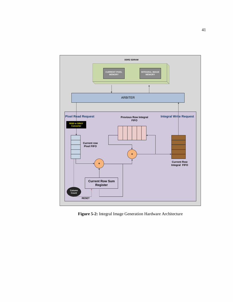
5.2 Implementation

The Integral Image unit consists of a FIFO termed Current_Pixel_FIFO to store the gray

values of pixels in the current image and a Write_Integral_FIFO to store and write back the

integral image values into Integral_Image_Memory residing in DDR2 SDRAM. Therefore, the

arbitration is between the reading of current pixels and writing of Integral values. A FIFO termed

Previous_Row_Integral_FIFO stores the integral values found in the previous row. The

Current_Row_Sum_Register accumulates the sum of the integral values of the current row upto

the current pixel as the row is scanned pixel by pixel. The Final Integral value written into the

Current_Integral_FIFO is the sum of the value in the Current_Row_Sum_Register and the value

read from the Previous_Row_Integral_FIFO ( integral value of pixel right above the current

pixel). This value is also written back into the Previous_Row_Integral_FIFO for use by the next

row in the image. A column count is maintained in order keep track of the end of row. This

architecture is shown in Figure 5-2.

41

Current Row Sum

Register

Current row

Pixel FIFO

Previous Row Integral

FIFO

+

+

Current Row

Integral FIFO

ARBITER

CURRENT PIXEL

MEMORY

INTEGRAL IMAGE

MEMORY

DDR2 SDRAM

Column

Count

RESET

Pixel Read Request Integral Write Request

RGB to GRAY

Converter

Figure 5-2: Integral Image Generation Hardware Architecture

42

Chapter 6

TRACKING UNIT

6.1 Discussion

The Tracking Unit detects boxes that are likely to represent persons in a frame and

assigns ids depending on the scenario. The protocol for assigning ids is as follows:

A new id is assigned to newly found blobs.

The same id is retained for those blobs that closely match the blobs in the previous frame.

A single id is given to a group of people when a merge is detected.

The id corresponding to people who split from a group is determined from a history table

and assigned correspondingly.

The dispense unit sends boxes found in the current frame to the Person Detection module. The

Person Detection module filters boxes using a predefined aspect ratio threshold that suits humans

inside a closed environment and sends the boxes that cross the threshold to the Centroid

Processing Unit.

The Centroid Processing Unit is designed based on the algorithm proposed by Tao Yang

et.al [12]. This algorithm is effective in quickly detecting the above mentioned four cases based

on Euclidean distance matrix calculation and a correspondence matrix calculation. In order to

handle Merge and Split cases, feature extraction is necessary. The Integral Image Unit discussed

in Chapter 5 generates the Integral Image value of every pixel in the image and stores the results

in Integral_Image_Memory. The integral of a box is used as the distinguishing feature to resolve

splits. The following sections discuss the functioning of each block in detail.

43

6.2 Tracking algorithm

Various tracking algorithms have been proposed in recent literature. Accurate and real

time object tracking will greatly improve the performance of object recognition, activity analysis,

and high-level event understanding [12,13,14]. However most approaches have a common layer

of image processing steps- background estimation, segmentation, feature extraction and

association. Stan Li et.al [14] proposed an algorithm that requires a minimal amount memory and

can handle cases of partial and total occlusion. This is suitable for implementation on current

FPGAs because of the abundance of on-chip SRAM memory resources. The tracking scheme

proposed in this work uses two layers of object tracking. The primary layer is based on Mean

Shift tracking using centroids and the secondary layer uses integral image features to distinguish

individuals following an occlusion event. The algorithm is summarized below.

A correspondence process tries to associate the current centroids with the centroids in

history table (global centroids). A distance matrix is formed between the current centroids and the

global centroids. Initially, the correspondence matrix between the current centroids and the global

centroids contains zeros. Now, the minimum distance in each row is found and the corresponding

location in the correspondence matrix is incremented by one. Similarly the minimum distance in

each column is found and the corresponding location in the correspondence matrix is incremented

by one. Three possible values may be found in the element of the correspondence matrix – Zero

indicates no selection, One indicates one selection happens, and Two indicates track and the

measure select each other both. This leads us to one of the following conclusions based on the

scenario:

A track is not associated to any measure (All the elements in a row are zero).

A measure is not associated to any track (All the elements in a column are zero).

44

A track is associated to more than one measure (More than one element in a row

is larger than zero).

A measure is associated to more than one track (More than one element in a row

is larger than zero).

A measure is associated to a track (The element value is two and the rest of the

elements in the row and column are zero).

To handle merges and splits two separate buffers are constructed while scanning the

correspondence matrix - The Merge Buffer which stores the ids of the centroids in the previous

frame that are merged in the current frame and The Split Buffer which stores the id from which

the current centroid is split. At the end of processing the correspondence matrix, each centroid is

sent to a corresponding Processing Unit in the Update Unit which decides the way in which the

Global block would be updated. Figure 6-1 shows the architecture of the Tracking Unit that is

implemented.

45

6.3 Implementation

CURRENT

BLOCK

GLOBAL BLOCK

PERSON

DETECTOR

CENTROID

PROCESSING

UNIT

UPDATE

UNIT

INTEGRAL

Receive/

Transmit

ADDRESS

CALC

DISPENSE UNIT

DDR2 SDRAM

Box

Memory

Integral

Memory

Figure 6-1: Tracking Unit Architecture

46

6.3.1 Person Detection

>

>

Ht

Wt

Centroid_X = 0.5*(min_X+max_X)

Centroid_Y = 0.5*(min_Y+max_Y)

Bounding Box FIFO

{min_X,min_Y,

max_X,max_Y}

Valid Centroid FIFO

Write Enable

(x,y)

Figure 6-2: Person Detection Architecture

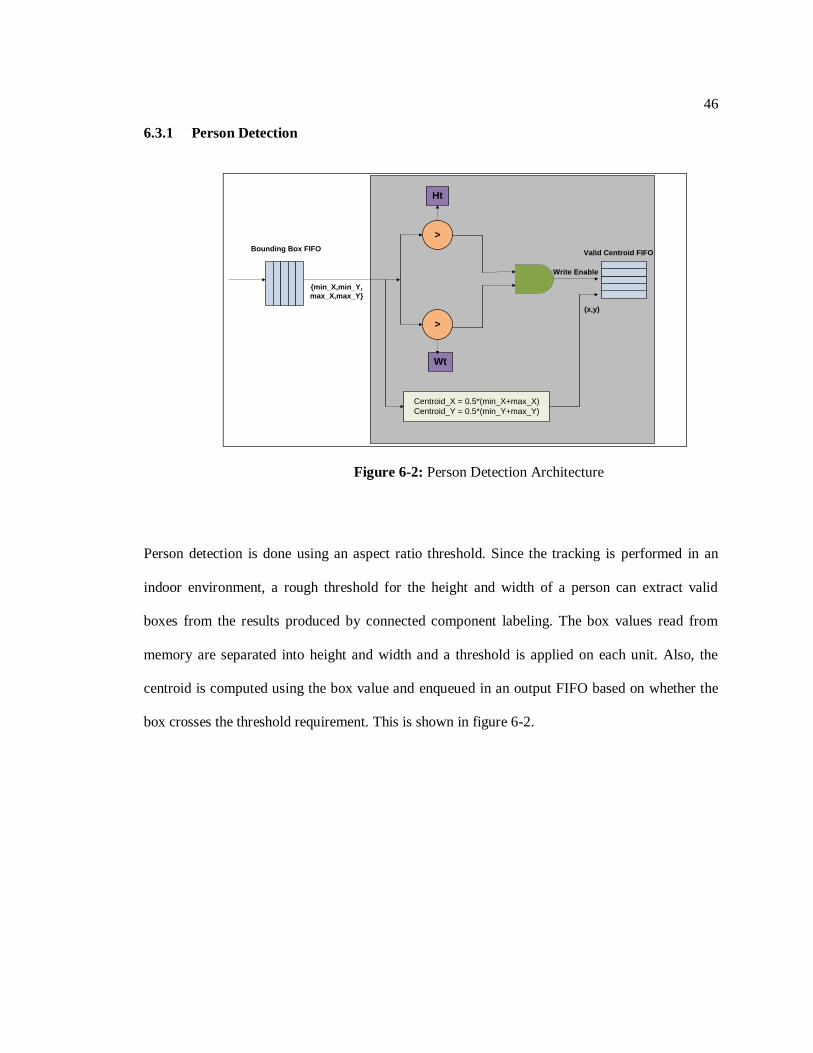
Person detection is done using an aspect ratio threshold. Since the tracking is performed in an

indoor environment, a rough threshold for the height and width of a person can extract valid

boxes from the results produced by connected component labeling. The box values read from

memory are separated into height and width and a threshold is applied on each unit. Also, the

centroid is computed using the box value and enqueued in an output FIFO based on whether the

box crosses the threshold requirement. This is shown in figure 6-2.

47

6.3.2 Centroid Processing Unit (CPU)

Euclidean Distacne

Calculator

Sqrt((x2-x1)2 + (y2-y1)2)

Euclidean Distance

Calculator

Sqrt((x2-x1)2 + (y2-y1)2)

Correspondence

Matrix Calculator

MERGE BUFFER

SPLIT BUFFER

Global

Centroid

Global

Count

Global

Integral

Global

ID

Global

Occlusion

Centroid FIFO

CPU

Figure 6-3: Centroid Processing Unit

The Centroid Processing Unit (CPU) as highlighted in Figure 6-3 reads two centroids

simultaneously from the Global Centroid buffer (stores centroids of ids found over the previous

frames) and calculates the Euclidean Distance of each of centroid in the current frame. Based on

this a Correspondence matrix is also calculated in a pipelined fashion to fill the Merge Buffer and

Split Buffer accordingly. At the end of reading all centroids from the Centroid FIFO and Global

Centroid buffer, the status (new, matching, merge or split) of each Centroid in the current frame

is obtained from the Merge and Split Buffers.

48

6.3.3 Current Block

Current Centroid FIFO

Current Integral FIFO

From CPU

Update UnitRequest

Grant

Request

Grant

Integral

Rx/Tx

Figure 6-4: Current Block

The Current Block stores the Centroids and the Integral Image values corresponding to an

NxN box around each centroid. The Integral values are obtained from memory. Therefore, as the

centroids are being filled into the Current Centroid FIFO, Integral Requests are made to the

Integral Rx/Tx unit. When a request is made by the Update Unit for an Integral value around a

particular centroid, the Current block sends the corresponding integral value when it is ready.

This is shown in Figure 6-4.

6.3.4 Integral Receive/Transmit

Integral Rx/Tx

Box

Calculator

Integral

Calculator

To

DDR2 Memory

From DDR2

Memory

From Current

Block

To Current

Block

Figure 6-5: Integral Receive/Transmit

49

The Integral Rx/Tx Unit as shown in Figure 6-5, has two state machines. The Box

calculator calculates an NxN box (N specified apriori) given a centroid(from Current block).

Hence four read requests are made to Integral_Image_Memory with the translated memory

addresses of each of the four coordinates. The second state machine termed Integral Calculator

receives the four integral values corresponding to the four coordinates from

Integral_Image_Memory and calculates the Integral Image value of the box and sends the value

to the current block.

6.3.5 Update Unit

MERGE/

SPLIT

ENCODER

DECODER

Fro

m M

erg

e B

uff

er

Fro

m S

plit

Bu

ffe

r

3'bxxxNew ID PU

Split PU

Merge PU

No Change PU

From Current Block

Global

Centroid

Global

Count

Global

Integral

Global

ID

Global

Occlusion

ID PROCESSING

UPDATE UNIT

Figure 6-6: Update Unit

50

The Merge Split status of each centroid is encoded and sent to the Update Unit. Based on

the status of each centroid, the Update Unit‟s job is to retrieve or assign an id to each centroid.

The Update Unit gets all the required information from the Global block and Current block and

updates the centroids with their corresponding ids accordingly. The architecture of this block is

shown in Figure 6-6.

New ID PU: When a centroid goes through the New ID PU, a new id is assigned to the centroid.

The Global Buffer is updated as follows:

Global Centroid is updated with Current Centroid.

Global Count is updated with 1.

Global Integral is updated with Current Integral.

Global id is updated with a new id in MSB(new id is now incremented)

Global Occlusion is updated with 0.

No Change PU: When a centroid goes through the No Change PU, following updates are done

Global Centroid is updated with Current Centroid.

Global Count is not updated

Global Integral is updated with Current Integral if Global Occlusion is 0

or else it is not updated.

Global id is not updated

Global Occlusion not updated.

Merge PU: When a centroid goes through the Merge PU, it means it has merged with another ID.

The Merge PU in this case assigns a single ID to the group. The Merge Buffer stores information

about the ids (in the previous frame) that are now merged. The Merge PU computes the smallest

among these ids and updates the Global Buffer as follows:

With the smallest id as the reference,

51

The Global Centroid is updated with Current Centroid

The Global Count is added with the number of ids that have merged.

The Global Integral is not updated

The Global Id is updated with the smallest ID as MSB and the rest of the IDs

following it

Global Occlusion is updated with 1 for all the merged ids.

Split PU: When a centroid goes through the Split PU, it means it has split from a group

represented by a single ID in the previous frame. The Split PU has to use the integral image

values in this case as the distinguishing feature. The Split buffer stores the ID from which the

current centroid is split. Therefore, all ids corresponding to this entry in the Global ID buffer are

read and their integral image values obtained from the current block are compared and the best

matching integral(found by simple differencing) is identified. The update of the Global buffer is

as follows:

With the matching id as reference,

The Global Centroid is updated with Current Centroid.

The Global count is updated with 1 and global count of the split id is

decremented by 1.

The Global integral is updated with current integral

The Global Id is updated with matching id.

The Global Occlusion is updated with 0.

When the count corresponding to the split id reaches 0, it means all the ids that were merged are

split now and an update needs to be done to this particular id as follows:

The Global Centroid is updated with Current Centroid.

The Global count is updated with 1

52

The Global integral is updated with current integral

The Global Id is updated with split id as MSB and rest are zeros.

The Global Occlusion is updated with 0.

A collection of snapshots from a video demo is shown in Figure 6-7.

Figure 6-7: A collection of snapshots from a video demo showing every fifth frame

53

Chapter 7

CONCLUSION

With Video and Image Processing technology evolving rapidly, and the requirement for

advanced image processing techniques that must include streaming capability, low latency, and

lossless compression[16], FPGAs offer an opportunity to balance high performance, flexibility,

upgradeability, and low development costs.

This thesis describes the implementation of a complete embedded tracking system on a

Virtex-5 FPGA. The system utilizes plug and play modules that can be controlled by an

embedded processor .The system also accounts for the bandwidth and latency characteristics of a

realistic embedded system accessing a DDR memory device. Connected component analysis

which is an integral part of any Image Processing application, was implemented in a novel

fashion by slicing the input image and merging the results from each slice in the end. The results

outperformed reference software implementations and other recent hardware implementations by

a wide margin. A streaming design methodology that minimizes storage requirements was

utilized to design other units in the system including the Background Estimation Unit, the

Filtering Unit and the Integral Image Generation unit. As the Tracking Unit has minimal memory

requirement, it mapped efficiently to the abundant Block RAM resources available on the

Virtex 5 fx130t FPGA device.

In conclusion, FPGAs are excellent solutions for realizing high performance Image and

Video Processing applications including Video Surveillance, Real-time monitoring, Medical

Imaging, and Tracking.

54

REFERENCES

[1] A. Yilmaz, O. Javed, and M. Shah, “Object tracking: A survey,” ACM Comput. Surv.,

vol. 38, no. 4, pp. 1–45, 2006.

[2] Ali, A. And Aggarwal, J. 2001. Segmentation and recognition of continuous human

activity. In IEEEWorkshop on Detection and Recognition of Events in Video. 28–35.

[3] Appiah, K., and Hunter, A., “A single-chip FPGA implementation of real-time adaptive

background model,” IEEE International Conference on Field-Programmable

Technology, pp. 95-102, December 2005.

[4] Ashley Rasquinha and N. Ranganathan, “C3L: A Chip for Connected Component

Labeling”, in the Proceedins of the 10th International Conference on VLSI Design: VLSI

in Multimedia Applications, p.446, (4-7 January 1997).

[5] D.G. Bailey, “Raster Based Region Growing,” in Proceedings of the 6th

New Zealand

Image Processing Workshop, Lower Hutt, New Zealand, August 1991, pp. 21–26.

[6] H.M. Alnuweiti and V.K. Prasanna, “Parallel architectures and algorithms for image

component labeling”, IEEE Transactions on Pattern Analysis and Machine Intelligence,

14:(10) 1014-1034 (1992).

[7] D. Crookes and K. Benkrid, “An FPGA Implementation of Image Component Labeling”,

in Reconfigurable Technology: FPGAs for Computing and Applications, SPIE 3844: 17-

23 (August 1999).

[8] D.G. Bailey and C.T. Johnston, “Single Pass Connected Components Analysis”, in Image

and Vision Computing, New Zealand, Hamilton, New Zealand, 282-287 (6-7 December,

2007)

55

[9] C.T. Johnston, and D.G. Bailey, “FPGA implementation of a Single Pass Connected

Components Algorithm”, in IEEE International Symposium on Electronic Design, Test

and Applications (DELTA 2008), Hong Kong, 228-231 (23-25 January 2008).

[10] Appiah,Kofi and Hunter, Andrew and Dickinson, Patrick and Owens, Jonathan (2008) “A

run-length based connected component algorithm for FPGA implementation”. In:

International Conference on Field-Programmable Technology 2008, 7th - 10th

December, Taipei, Taiwan.

[11] Viola,Paul; Jones,Michael (2002). “Robust Real-time Object Detection” International

Journal of Computer Vision.

[12] A. Amer, E. Dubois, and A. Mitiche, Real-time system for high-level video

representation: application to video surveillance,in Proc. SPIE Int. Symposium on

Electronic Imaging, Conf. on Visual Communication and Image Processing (VCIP),

Santa Clara, USA, vol. 5022, pages 530-541, Jan. 2003.

[13] Collins et al. A System for Video Surveillance and Monitoring.VSAM Final Report,

Technical report CMU-RI-TR- 00-12, Carnegie Mellon University, May, 2000.

[14] Fengjun Lv, Jinman Kang, Ram Nevatia, Isaac Cohen, and Gérard Medioni, Automatic

Tracking and Labeling of Human Activities in a Video Sequence, Proceedings of the 6th

IEEE International Workshop on Performance Evaluation of Tracking and Surveillance

(PETS04), Prague, Czech Republic, May, 2004.

[15] Tao Yang, Stan Z.Li, Quan Pan and Jing Li, “Real-time Multiple Objects Tracking with

Occlusion Handling in Dynamic Scenes”, Proceedings of the 2005 IEEE Computer

Society Conference on Computer Vision and Pattern Recognition (CVPR‟05) – Volume

1, p.970-975, June 20-26,2005.

[16] White Paper, Video and Image Processing Design Using FPGAs. Altera.March 2007