an h-based approach for robust sensor localization
TRANSCRIPT

HAL Id: hal-01266215https://hal.archives-ouvertes.fr/hal-01266215
Submitted on 7 Mar 2017
HAL is a multi-disciplinary open accessarchive for the deposit and dissemination of sci-entific research documents, whether they are pub-lished or not. The documents may come fromteaching and research institutions in France orabroad, or from public or private research centers.
L’archive ouverte pluridisciplinaire HAL, estdestinée au dépôt et à la diffusion de documentsscientifiques de niveau recherche, publiés ou non,émanant des établissements d’enseignement et derecherche français ou étrangers, des laboratoirespublics ou privés.
An H∞-based approach for robust sensor localizationUsman Khan, Anton Korniienko, Karl Henrik Johansson
To cite this version:Usman Khan, Anton Korniienko, Karl Henrik Johansson. An H∞-based approach for robust sensorlocalization. 54th IEEE CDC, Dec 2015, Osaka, Japan. pp.1719-1724, 10.1109/CDC.2015.7402458.hal-01266215

An H∞-based approach for robust sensor localization
Usman A. Khan, Anton Korniienko, and Karl H. Johansson
Abstract— In this paper, we consider the problem of sensorlocalization, i.e., finding the positions of an arbitrary number ofsensors located in a Euclidean space, Rm, given at least m+1 an-chors with known locations. Assuming that each sensor knowspairwise distances in its neighborhood and that the sensors liein the convex hull of the anchors, we provide a DIstributedLOCalization algorithm in Continuous-Time, named DILOC-CT, that converges to the sensor locations. This representationis linear and is further decoupled in the coordinates.
By adding a proportional controller in the feed-forward loopof each location estimator, we show that the convergence speedof DILOC-CT can be made arbitrarily fast. Since a large gainmay result into unwanted transients especially in the presenceof disturbance introduced, e.g., by communication noise in thenetwork, we use H∞ theory to design local controllers thatguarantee certain global performance while maintaining thedesired steady-state. Simulations are provided to illustrate theconcepts described in this paper.
I. INTRODUCTION
Localization is often referred to as finding the position ofa point in a Euclidean space, Rm, given a certain numberof anchors, with perfectly known positions, and point-to-anchor distances and/or angles. Traditionally, distance-basedlocalization has been referred to as trilateration, whereasangle-based methods are referred to as triangulation. Tri-lateration is the process of finding a location in Rm, givenonly the distance measurements to at least m+ 1 anchors,see Fig. 1 (Left). With m + 1 sensor-to-anchor distances,the nonlinear trilateration problem is to find the intersectionof three circles. Triangulation, Fig. 1 (Right), employs theangular information to find the unknown location.
The literature on localization is largely based on thetriangulation and trilateration principles, or in some cases,a combination of both. Recent work may be broadly char-acterized into centralized and distributed algorithms, see [1]where a comprehensive coverage of cooperative and non-cooperative strategies is provided. Centralized localizationalgorithms include: maximum likelihood estimators, [2], [3];multi-dimensional scaling (MDS), [4], [5]; optimization-based methods to include imprecise distance information,see [6]; for additional work, see [7]–[9]. Optimization basedtechniques can be found in [10], [11] and references therein,whereas, polynomial methods are described in [12].
UAK is with the Department of Electrical and Computer Engineering atTufts University, Medford, MA 02155, USA, [email protected] work is supported by an NSF Career award # CCF-1350264.
AK is with Laboratoire Ampere, Ecole Centrale de Lyon, 69134 EcullyCedex, France, [email protected]. His work issupported by a grant from la Region Rhone-Alpes.
KHJ is with the KTH ACCESS Linnaeus Center, School of ElectricalEngineering, Royal Institute of Technology (KTH), Stockholm, Sweden,[email protected]. His work is supported by the Knut and AliceWallenberg Foundation and the Swedish Research Council.
c
1
2
3dc1
dc2
dc3h
c
12
d12dh1
dh2
dc1
dc2
θc1θc2
Fig. 1. Localization in R2, anchors: red triangles; unknown location:blue circle. (Left) Trilateration–the unknown location is at the intersectionof three circles. (Right) Triangulation–the line segments, h, dc1, dc2, dh1,and dh2, are computed from trigonometric operations.
Distributed localization algorithms can be characterizedinto two classes: multilateration and successive refinements.In multilateration algorithms, [13], [14], each sensor es-timates its distance from the anchors and then calculatesits location via trilateration; multilateration implies that thedistance computation may require a multi-hop communi-cation. Distributed multidimensional scaling is presentedin [15]. Successive refinement algorithms that perform aniterative minimization of a cost function are presented in,e.g., [16], which discusses an iterative scheme where theyassume 5% of the nodes as anchors. Reference [17] discussesa Self-Positioning Algorithm (SPA) that provides a GPS-freepositioning and builds a relative coordinate system. Otherrelated work also consists of graph-theoretic approaches [18],[19], and probabilistic methods, [20], [21].
Of significant relevance to this paper is Ref. [22], whichdescribes a discrete-time algorithm, named DILOC, assum-ing a global convexity condition, i.e., each sensor lies inthe convex hull of at least m + 1 anchors in Rm. Asensor may find its location as a linear-convex combinationof the anchors, where the coefficients are the barycentriccoordinates; attributed to August F. Mobius, [23]. However,this representation may not be practical as it requires long-distance communication to the anchors. To overcome thisissue, each sensor finds m + 1 neighbors, its triangulationset, such that it lies in their convex hull and iterates on itslocation as a barycentric-based representation of only theneighbors. Assuming that each sensor can find a triangulationset, DILOC converges to the true sensor locations. Ref. [22]analyzes the convergence and provides tests for findingtriangulation sets with high probability in a small radius.
In this paper, we provide a continuous-time analog ofDILOC-DT in [22], that we call DILOC-CT, and show thatby using a proportional controller in each sensor’s locationestimator, the convergence speed can be increased arbitrarily.Since this increase may come at the price of unwanted
transients especially when there is disturbance introduced bythe network, we replace the proportional gain with a dynamiccontroller that guarantees certain performance objectives. Wethus consider disturbance in the communication network thatis incurred as zero-mean additive noise in the informationexchange. In this context, we study the disturbance rejectionproperties of the local controllers and tune them to withstandthe disturbance while ensuring some performance objectives.Our approach is based on H∞ design principles and uses theinput-output approach, see e.g., [24]–[27].
Notation: The superscript, ‘T ’, denotes a real matrixtranspose while the superscript, ‘∗’, denotes the complex-conjugate transpose. The N ×N identity matrix is denotedby IN and the n × m zero matrix is denoted by 0n×m.The dimension of the identity or zero matrix is omittedwhen it is clear from the context. The diagonal aggregationof two matrices A and B is denoted by diag(A,B). TheKronecker product, denoted by ⊗, between two matrices, Aand B, is defined as A ⊗ B = [aijB]. We use Tx→y(s)to denote the transfer function between an input, x(t),and an output, y(t). With matrix, G, partitioned into fourblocks, G11, G12, G21, G22, G ? K denotes the Redhefferproduct, [31], i.e.,
G ?K = G11 +G12K (I −G22K)−1G21.
Similarly, K ? G = G22 + G21K (I −G11K)−1G12. For
a stable LTI system, G, ‖G‖∞ denotes the H∞ normof G. For a complex matrix, P : σ (P ) denotes its maxi-mal singular; λi(P ) denotes the ith eigenvalue; and ρ(P )denotes its spectral radius. Finally, the symbols, ’≥’ and ’>,denote positive semi-definiteness and positive-definiteness ofa matrix, respectively.
We now describe the rest of the paper. Section II de-scribes the problem, recaps DILOC-DT, and introduces thecontinuous-time analog, DILOC-CT. Section III derives theconvergence of DILOC-CT with a proportional gain andinvestigates disturbance-rejection. In Section IV, we describedynamic controller design using the H∞ theory according tocertain objectives that ensure disturbance rejection. Section Villustrates the concepts and Section VI concludes the paper.
II. PRELIMINARIES AND PROBLEM FORMULATION
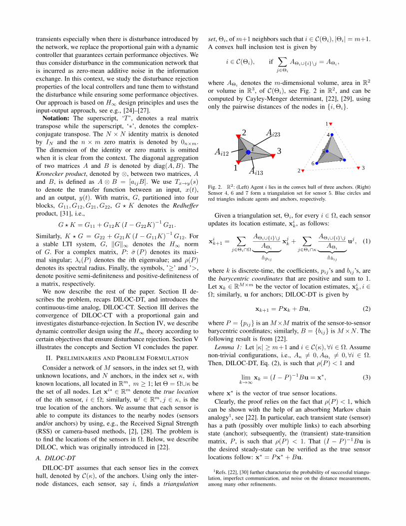
Consider a network of M sensors, in the index set Ω, withunknown locations, and N anchors, in the index set κ, withknown locations, all located in Rm, m ≥ 1; let Θ = Ω∪κ bethe set of all nodes. Let xi∗ ∈ Rm denote the true locationof the ith sensor, i ∈ Ω; similarly, uj ∈ Rm, j ∈ κ, is thetrue location of the anchors. We assume that each sensor isable to compute its distances to the nearby nodes (sensorsand/or anchors) by using, e.g., the Received Signal Strength(RSS) or camera-based methods, [2], [28]. The problem isto find the locations of the sensors in Ω. Below, we describeDILOC, which was originally introduced in [22].
A. DILOC-DTDILOC-DT assumes that each sensor lies in the convex
hull, denoted by C(κ), of the anchors. Using only the inter-node distances, each sensor, say i, finds a triangulation
set, Θi, of m+1 neighbors such that i ∈ C(Θi), |Θi| = m+1.A convex hull inclusion test is given by
i ∈ C(Θi), if∑j∈Θi
AΘi∪i\j = AΘi ,
where AΘi denotes the m-dimensional volume, area in R2
or volume in R3, of C(Θi), see Fig. 2 in R2, and can becomputed by Cayley-Menger determinant, [22], [29], usingonly the pairwise distances of the nodes in i,Θi.
i
1
2
3
Ai23
Ai12
Ai13
1
2 3
4
5
67
Fig. 2. R2: (Left) Agent i lies in the convex hull of three anchors. (Right)Sensor 4, 6 and 7 form a triangulation set for sensor 5. Blue circles andred triangles indicate agents and anchors, respectively.
Given a triangulation set, Θi, for every i ∈ Ω, each sensorupdates its location estimate, xik, as follows:
xik+1 =∑
j∈Θi∩Ω
AΘi∪i\j
AΘi︸ ︷︷ ︸,pij
xjk +∑
j∈Θi∩κ
AΘi∪i\j
AΘi︸ ︷︷ ︸,bij
uj , (1)
where k is discrete-time, the coefficients, pij’s and bij’s, arethe barycentric coordinates that are positive and sum to 1.Let xk ∈ RM×m be the vector of location estimates, xik, i ∈Ω; similarly, u for anchors; DILOC-DT is given by
xk+1 = Pxk +Bu, (2)
where P = pij is an M×M matrix of the sensor-to-sensorbarycentric coordinates; similarly, B = bij is M×N . Thefollowing result is from [22].
Lemma 1: Let |κ| ≥ m+1 and i ∈ C(κ),∀i ∈ Ω. Assumenon-trivial configurations, i.e., Aκ 6= 0, AΘi 6= 0,∀i ∈ Ω.Then, DILOC-DT, Eq. (2), is such that ρ(P ) < 1 and
limk→∞
xk = (I − P )−1Bu = x∗, (3)
where x∗ is the vector of true sensor locations.Clearly, the proof relies on the fact that ρ(P ) < 1, which
can be shown with the help of an absorbing Markov chainanalogy1, see [22]. In particular, each transient state (sensor)has a path (possibly over multiple links) to each absorbingstate (anchor); subsequently, the (transient) state-transitionmatrix, P , is such that ρ(P ) < 1. That (I − P )−1Bu isthe desired steady-state can be verified as the true sensorlocations follow: x∗ = Px∗ +Bu.
1Refs. [22], [30] further characterize the probability of successful triangu-lation, imperfect communication, and noise on the distance measurements,among many other refinements.

B. DILOC-CT
We now provide DILOC-CT, a continuous-time analog toDILOC-DT. To this aim, let xi(t) denote the m-dimensionalrow-vector of sensor i’s location estimate, where t ≥ 0 isthe continuous-time variable. Since the anchors’ locationsare known, we have uj(t) = uj ,∀t ≥ 0, j ∈ κ. Borrowingnotation from Section II-A, DILOC-CT is given by, where (t)is dropped in the sequel for convenience:
xi = −xi + ri; ri ,∑
j∈Θi∩Ω
pijxj +∑
j∈Θi∩κbijuj , (4)
and Θi is the triangulation set at sensor i. Note that Θi maynot contain any anchor, in which case |Θi ∩ Ω| = m + 1,and |Θi ∩ κ| = 0. In other words, a sensor may not haveany anchor as a neighbor and the barycentric coordinates areassigned to the neighboring sensors, with unknown locations.
In order to improve the convergence rate, we may adda proportional gain, α ∈ R, in the feed-forward loop ofeach sensor’s location estimator, denoted by an identicalsystem, Ts, at each sensor:
Ts : xi = α(−xi + ri). (5)
We now assume that the received signal at each sensor incursa zero-mean additive disturbance, zi(t), whose frequencyspectrum lies in the interval, [ω−z , ω
+z ]. With this disturbance,
the location estimator is given by
xi = α(−xi + ri + zi). (6)
Here, zi(t) can be thought of as communication noise thateffects the information exchange. Note that Eq. (4) is specialcase of Eq. (6) with α = 1 and z = 0. Finally, we replacethe proportional gain, α, with a local controller, K(s). Theoverall architecture is depicted in Fig. 3, where we separatethe desired signal, ri, and the disturbance, zi, as two distinctinputs to each Ts.
1/sK(s)xi(t)
ri(t)
Networkyi(t)εi(t)
zi(t)Ts
Fig. 3. DILOC-CT architecture
The contributions of this paper are as follows: First, weshow that DILOC-CT converges to the true sensor locationsand characterize the range of gains that ensures this conver-gence. We then study the disturbance rejection properties ofthe proportional gain. This analysis is provided in Section III.Second, we note that an arbitrary high proportional gain mayresult in unwanted transients and disturbance amplification.In order to add design flexibility and guarantee certainperformance objectives, we replace the proportional gain, α,with local controllers, K(s). We use H∞ design procedure
to derive these local controllers meeting global objectives.This analysis is carried out in Section IV. Finally, we studythe disturbance rejection properties of the local controllerswith the help of the H∞ design in Sections IV and V.
III. DILOC-CT WITH PROPORTIONAL GAIN
We now analyze the convergence properties of the propor-tional gain controller without disturbance in Eq. (5). Let x(t)collect the location estimates at the sensors and let u collectthe true locations of the anchors. Borrowing notation fromSection II-A, we use the matrices, P and B, to denotethe corresponding barycentric coordinates. Eq. (5) can beequivalently written in the following matrix form:
x = −α(I − P )x + αBu , Pαx +Bαu. (7)
We have the following result.Lemma 2: If ρ(P ) < 1, then <λi(Pα) < 0,∀i, α > 0.
Proof: Let λi(P ) = ai +√−1bi for some ai, bi ∈ R,
and note that |ai| < 1,∀i, since ρ(P ) < 1, then
λi(I − P ) = 1− ai −√−1bi, (8)
and the lemma follows for any α > 0.The following theorem studies the DILOC-CT convergence.
Theorem 1: DILOC-CT, Eq. (7), converges to the truesensor locations, x∗, for all α > 0, i.e.,
limt→∞
x(t) = (I − P )−1Bu = x∗. (9)Proof: From Lemma 2, we have <λi(Pα) < 0,∀i.
Starting from Eq. (7), we get
x(t) = ePαtx(0) +
∫ t
0
ePαταBu(t− τ)dτ,
= ePαtx(0) + P−1α
(ePαt − I
)αBu,
which asymptotically goes to (since limt→∞ ePαt = 0)
limt→∞
x(t) = −P−1α αBu = −(−α(I − P ))−1αBu,
and the theorem follows.That the convergence speed is exponential in α > 0can also be easily verified. In fact, the real part of theeigenvalues of Pα move further into the left-half planeas α increases. However, in the presence of network-baseddisturbances, zi(t)’s, an arbitrarily large α also amplifies thedisturbance. To guarantee certain performance objectives, anatural extension is to replace the proportional (static) gainwith a dynamic controller, K(s). We study this scenariousing H∞ design in Section IV.
In the following, we analyze the disturbance rejection withthe proportional controller. To proceed, we use the fact thatDILOC-CT is decoupled in the coordinates. Hence, eachlocal system, Ts, see Eq. (5) and Fig. 3, can be analyzed percoordinate and the same analysis can be extended to othercoordinates. Recall that the network location estimate, x(t),is a M × m matrix where each column is associated to alocation coordinate in Rm. We let x to be an arbitrarilychosen column of x corresponding to one chosen dimen-sion. Similarly, we let z, r, ε, and y (signals in Fig. 3) torepresent M -dimensional vectors; for any of such vectors,the subscript i denotes the chosen coordinate at sensor i.

A. Rejection vs. Localization tradeoff, M = 1
We first consider the simplest case of DILOC-CT in R2,with static controller, K(s) = α, N = 3 anchors and onesensor, M = 1, see Fig. 2 (Left). In this case, the dynamicsof the overall network is equivalent to the dynamics, Tsin Eq. (5), of one sensor and a constant input ri definedby Eq. (4) with pij = 0. Since the H∞ design approachused in the next sections is frequency-based, the localizationperformance will be expressed thereafter in the frequencydomain. Since P = 0, we have ri =
∑bijuj , where uj is
the true location of the anchors and the performance (steady-sate error, convergence speed) is defined by the trackingperformance of the dynamics, Ts. Let us define a transferfunction, S(s), between the reference input, ri, and trackingerror, defined as εrefi , x∗i − xi, which for K = α is
S(s) = (1 +K(s) 1s )−1 = s(s+ α)−1. (10)
For all α > 0, S(s) is stable with a zero at the origin imply-ing 0 steady-state error for constant inputs. It is important tonote that the cutoff frequency, ωS , for which |S(jωS)| =
√2
2 ,is ωS = α. The magnitude of S is close to zero in theLow Frequency (LF) range (ω ωS) and approaches 1 inthe High Frequency (HF) range (ω ωS). Increasing αincreases the cutoff frequency of S implying an increase inthe convergence speed, which follows Theorem 1.
To proceed with the subsequent analysis, note that
Tzi→xi(s) = Tri→xi(s) = αs+α = 1− S(s) , T (s),
Tzi→yi(s) = Tri→yi(s) = αss+α = K(s)S(s) , KS(s).
(11)
The cutoff frequency, ωT , of T (s) is equal to the cutofffrequency, ωS , of S(s). Increasing α increases both ωTand ωS , and thus the bandwidth of T (s). Since the magnitudeof T (s) is equal to 1 in the LF range and decreases in theHF range, increasing α implies the transmission of a broaderfrequency range of disturbance, zi, on the output, xi. It istherefore not possible to increase the convergence speed anddisturbance rejection at the same time. This is also true forthe dynamic controller, K(s); we may, however, impose alarger slope of magnitude decay in T (s). Let us now considerthe transfer function, KS(s). In the HF range, |KS(s)| = α,and thus an increase in α amplifies the disturbance. A logicalextension is to consider a dynamic controller, K(s), whichis frequency-dependent such that it has a high gain in theLF range, for a good tracking performance; and a low gainin the HF range for a better disturbance rejection.
B. Rejection vs. Localization tradeoff, M > 1
To study the general case, let us define the global transferfunction, Sg
u→εref , as an M×N matrix between the input, u(anchors positions), and the network tracking error, definedby εref , x∗ − x. Note that we can write the input as u =u‖u‖ ‖u‖ , where ‖u‖ is the Euclidean norm of u. In this case,the tracking performance of the network could be evaluatedby the M × 1 transfer function:
Sg‖u‖→εref = Sgu→εref
u
‖u‖, Sg, (12)
whose j-th component, Sgj , is the transfer function betweenthe constant, ‖u‖, and j-th sensor’s tracking error, εrefj . Letus define additional global transfer functions as follows:
Tz→x(s) , T g(s), Tz→y(s) , KSg(s). (13)
The transfer functions T g and KSg are M ×M matrices,components of which, T gij and KSgij , represent transferfunctions between j-th sensor disturbance, zj , and i-th sensorlocation estimate, xi, and control signals, yi, respectively.
In general, the components of Sg , T g , and KSg aredifferent form the local dynamics, S, T , and KS. How-ever, increasing α has the same consequences as discussedbefore in the simple case. We illustrate this numerically2
in Fig. 4, which shows the maximal singular value, σ(·),of frequency responses of Sg , T g , and KSg for a networkof M = 20 sensors with P 6= 0 and for α varying form 1to 104. Briefly, σ(·) is a generalization of gain for MIMOsystems, [32], and its maximum value for a given frequencyis the maximum amplification between the Euclidean normsof input-output vectors (over all directions of applied inputvector). We observe that similar to the local case, M = 1,an increase of α increases the convergence speed but alsoincreases HF disturbance amplification.
100
105
-120
-100
-80
-60
-40
-20
0
20
Max
sin
gu
lar
valu
e
100
105
-100
-80
-60
-40
-20
0
20
40
frequency, rad/sec 10
010
5-40
-20
0
20
40
60
80
100
α =104
α =1
α =104α =104
α =1
α =1
Sg Tg KSg
Fig. 4. Maximal singular value of Sg , T g , and KSg vs. α
As in the case with M = 1, in order to reduce the HFdisturbance amplification, it is possible to use a dynamiccontroller, K(s), that decreases the maximum HF singularvalue of T g and KSg . However, the design of such controllerin the general case of M > 1 is a non-trivial problemand could result in poor performance (low speed, highoscillations) and a global system instability for some choiceof K(s). In fact, it is a special case of the decentralizedcontrol problem, which is proved to be NP-hard even in theLTI case, [33]. However, since the sensors are identical it ispossible to link the global network to the local dynamics andthen perform a local design by the traditional H∞ approach.This method is proposed in [26], [27] and is applied, withsome changes, to DILOC-CT in the next section.
2It is possible to compute the closed-form expressions of Sg , T g ,and KSg , e.g., by using the Lower Fractional Transformation algebra(LFT), [31], but this computation is beyond the scope of this paper.

IV. DILOC-CT: H∞ DESIGN
We now consider DILOC-CT introduced earlier in Sec-tion II-B with local controllers. We assume that the barycen-tric matrices, P and B, are given3. Our objective is todesign identical (local) controllers, K(s), to achieve, besidesthe global system stability, certain performance objectives,summarized in Table I. We note that the location estimatorat each sensor is identical and define the following globalsystem description for each coordinate, recall Eq. (11):
x = (IM ⊗ T (s)) rz, (14)
where rz = r + z = Px+Buu0 + z, and u0 = ‖u‖ , Bu =B uu0
. Next note that εref = x∗−x = (IM −P )−1Buu0−x,and ε = rz−x, from Fig. 3. We have the following relation: rz
εref
ε
=
P Bu IM−IM (IM − P )
−10
P − IM Bu IM
︸ ︷︷ ︸
H
xu0
z
.(15)
The local transfer function, T (s), identical at each sensor, is
T (s) =K(s) 1
s
1 +K(s) 1s
(16)
Given the representation in Eqs. (14) and (15), we have
T[u0z ]→
[εref
ε
] = (IM ⊗ T (s)) ? H, (17)
and Tu0→εref (s) = Sg(s), see Eq. (12). Furthermore, T g(s)and KSg(s) can be written in terms of Tz→ε(s) as
T g(s) =K(s)
sTz→ε(s), KSg(s) = K(s)Tz→ε(s). (18)
We formulate the following control design problem:Problem 1 (Control problem): Given the global system in
Eqs. (14) and (15), find the local controller, K(s), suchthat the global system is stable and satisfies the followingfrequency constraints:
σ (Sg (jω)) ≤ ΩS (ω) , in LF range,σ (T g (jω)) ≤ ΩT (ω) , in HF range,
σ (KSg (jω)) ≤ ΩKS (ω) , in HF range.(19)
We now briefly explain the frequency constraints. The firstconstraint, ΩS , ensures zero steady-state error and providesa handle on the speed of convergence. The second con-straint, ΩT , imposes a maximum bandwidth on T g , which, inturn, limits the disturbance amplification in high-frequency.The last constraint, ΩKS , reduces the amplification of noiseon the local input, y, to each sensor’s local dynamics inhigh-frequency. Specifics on these constraints are tabulatedin Table I and are further elaborated in Section V.
3Note that the controller design requires the knowledge of all barycentriccoordinates, P and B, which may be restrictive. However, we stress that theresulting controller is local and the procedure described here is critical to anyfuture work on decentralized design. In addition, computing the locations ata central location from the matrices, P and B, and then transmitting themto the sensors incurs noise in the communication that is not suppressed;this procedure is further susceptible to cyber attacks revealing the sensorlocations to an adversary.
TABLE IDILOC-CT DESIGN SPECIFICATIONS
Performance specs. Frequency constraint RangeZero steady-state Slope of +20 dB/dec for σ (Sg (jω)) LFConv. speed Cutoff freq. of σ(Sg) ≥ 10 rad/sec LFDisturbance −60 dB/dec slope for σ (T g (jω)) HFreduction −40 dB/dec slope for σ (KSg (jω)) HF
In order to solve the above control problem, we will usethe well-known input-output approach, which was introducedto deal with interconnected systems, see [24]–[27] for details.
A. Input-output Approach
We now describe the input-output approach over whichwe will formulate the DILOC-CT controller design problem.We use the concept of dissipitavity taken from [24]–[27], asimplified version of which is defined below.
Definition 1 (Dissipativity): An LTI, stable, and causaloperator, H , is strictly X,Y, Z-dissipative, where X =XT , Y, Z = ZT , are real matrices such that[
X YY T Z
]is full-rank; if ∃ ε > 0 such that for almost all ω > 0[
IH(jω)
]∗ [X YY T Z
] [I
H(jω)
]≤ −εI. (20)
If the inequality in Eq. (20) is satisfied with ε = 0, theoperator is said to be X,Y, Z-dissipative.
Consider a large-scale system represented as an intercon-nection, H , of identical subsystems, Ts:
p = (I ⊗ Ts) (q) ,
[qz
]= H
([pw
]), (21)
whereH =
[H11 H12
H21 H22
]is a finite-dimensional, stable LTI system, Ts = G?K, w(t)is the input vector, z(t) is the output vector, and q(t), p(t),are internal signals. The LTI systems, G and K, are finite-dimensional and are referred to as the local plant andcontroller. The global transfer function between externalinput, w, and output, z, is
Tw→z = (I ⊗ Ts) ? H,
and its H∞ norm is ensured by the local controller, K, bythe following theorem.
Theorem 2: Given η > 0, a stable LTI system, H , a localplant, G, and real matrices, X = XT ≥ 0, Y , Z = ZT , ifthere exist
(i) a positive-definite matrix, Q, such that H isdiag(Q⊗X,−η2I), diag (Q⊗ Y, 0) , diag (Q⊗ Z, I)-dissipative, and
(ii) a local controller, K, such that Ts = G ? K is strictly−Z,−Y T ,−X-dissipative,

then the local controller, K, ensures that the global sys-tem, (INs ⊗ Ts) ? H , is stable and
‖ (I ⊗ Ts) ? H‖∞ ≤ η. (22)
The proof of Theorem 2 can be found in [26], [27], andit relies on a version of the graph-separation theorem usedin [24] for global stability and an S-procedure, [34], forglobal performance. It can also be seen as a generalizationof the Kalman-Yakubovich-Popov lemma, [35].
B. Local Control for Global Performance
Note that based on the properties of the H∞ norm:∥∥∥∥ T11 T12
T21 T22
∥∥∥∥∞≤ η ⇒ ‖T11‖∞ ≤ η,
‖T22‖∞ ≤ η,
⇔ σ (T11 (jω)) ≤ ησ (T22 (jω)) ≤ η ,∀ω ∈ R+,
(23)
Theorem 2 is applicable to the system in Eqs. (14) and (15) tofind a controller, K, ensuring a global bound, η, on the H∞norm of, in this case, T11 = Sg and T22 = Tz→ε. However,such imposed constraints are frequency-independent. Wenow present a result allowing to impose frequency-dependentbounds, Eq. (19), constructed with the help of local transferfunctions, KS, S, or T , and constant gains. Consider thefollowing augmented localization system:[
xx
]= (IM+1 ⊗ T (s))
[rr
],[
rr
εref
ε
]=
[ l 0 g1l 0lBu P g1lBu g3I
g−11 lP −g−1
1 I lP 0
g2lBu g2(P−IM ) g2g1lBu g2g3I
]︸ ︷︷ ︸
H
[xxuz
],
(24)with real positive scalars, g1, g2, g3, l = 1
1+β , 0 < β 1, P = (IM − P )
−1Bu, and one additional local sensor
dynamics, T (s), with additional input, r, and output, x.The main result of this paper is now provided in the
following theorem that solves Problem 1 following a similarargument as in Section IV-A.
Theorem 3 (Control Design): Given η > 0, the systemdescribed in Eq. (24), and real scalars, X ≥ 0, Y, Z ≤ 0, ifthere exists a positive-definite matrix, Q ∈ R(M+1)×(M+1),such that
(i) H is
diag(XQ,−η2I
), diag (Y Q, 0), diag (ZQ, I)-
dissipative,and a local controller, K, such that:(ii) T (s) is strictly −Z,−Y,−X-dissipative with‖T (s)‖∞ < 1, and T (s) =
(T (s) + Y
X
)√X2
Y 2−XZ ;(iii) |S (jω)| ≤ η−1ΩS (ω) , in the LF range;(iv) |KS (jω) | ≤ η−1g2g3 min ΩKS (ω) , ωΩT (ω) , in
the HF range;
then the local controller K solves the Problem 1.
Proof: Let us define weighted version of input-outputsignals of the original system in Eq. (15) as:
εref = g−11 εref ,
ε = g2ε,
z = g−13 z,
u = g−11 (S + β)u0.
Based on this notation, one can define the following relation:
T[uz ]→
[εref
ε
] = W1T[u0z ]→
[εref
ε
]W2,
with4 W1 =[g−11 00 g2IM
]and W2 =
[g1(S(s)+β)−1 0
0 g3IM
].
Since S(s) = T (s) − 1, the matrix transfer function, W2,can be represented in the form of an interconnection (LFT)of one system T (s):
W2 = T (s) ? HW ,
with HW =
l g1l 0l g1l 00 0 g3
.The global transfer function, Eq. (15), is an LFT of Msystems, T (s), and is defined by
T[u0z ]→
[εref
ε
] = (T (s)IM ) ? H.
The augmented system, T[uz ]→
[εref
ε
] = (IM+1 ⊗ T (s))?H ,
is an LFT of M + 1 systems, T (s), representing a seriesconnection of W1T[u0
z ]→[εref
ε
] and W2, and is given in
Eq. (24). The corresponding expression of H is computedbased on the LFT algebra, see Section 2.4 in [31], .
Note that the first two conditions of Theorem 3 correspondto the two conditions of Theorem 2. Applying Theorem 2,a controller that ensures second condition of Theorem 3,therefore, ensures the global transfer function bound:∥∥(T (s)IM+1) ? H
∥∥∞ =
∥∥∥∥W1T[u0z ]→
[εref
ε
]W2
∥∥∥∥∞≤ η.
Using Eq. (23), the last inequality implies ∀ω:
σ (Tu0→εref (jω)) ≤ η |S (jω) + β| ,
σ (Tz→ε (jω)) ≤ η (g2g3)−1.
(25)
For frequency range where β can be neglected comparedto |S (jω)|, condition (iii) of the Theorem 3 ensures the firstcondition of Problem 1. Note that in the HF range:
|KS (jω)| = |K (jω)|∣∣1− jωK (jω)
∣∣ ≈ |K (jω)| .
Therefore, together with Eq. (18), the condition (iv) impliesthe second and third conditions of the Problem 1.
4The reason of using parameter β is that in order to properly definethe H∞ norm, the weighting filters Wi should be stable transfer functions.Since S has zero at zero, Eq. (10) (because of presence of integrator inlocal sensor dynamics, see Fig 3), the weighting filter W2 would containintegrator and thus be unstable with β = 0. This is a classical problem inthe H∞ design, [32], which is practically solved by perturbing the pureintegrator, 1
s, by a small real parameter, β : 1
s→ 1
s+β.

Remark 1: Theorem 3 can be applied to efficiently designa controller, K, that solves Problem 1, if X , Y , and Z, arefixed. In this case, the first condition of Theorem 3 is aLinear Matrix Inequality (LMI) with respect to the decisionvariables, η and Q, and thus, convex optimization can beapplied to find the smallest η such that it is satisfied. Theconditions, (ii)-(iv), are ensured by the local traditional H∞design. However, if X , Y , and Z, are the decision variables,the underlying optimization becomes bilinear. In this case, aquasi-convex optimization problem for finding X , Y , and Z,that satisfy the condition (i) and relaxes the condition (ii) ofTheorem 3 is proposed in [26], [27] and is used thereafter.
Remark 2: The weighting filters, W1 and W2, are used toimpose frequency-dependent bounds on the global transferfunction magnitudes, Eq. (19), in a relative fashion, i.e.,global performance in Eq. (19) is ensured by the localsystem performance, see conditions (iii)-(iv) of Theorem 3.The reason for using different gains, gi, is to impose theconstraint on diagonal blocks, Tu0→εref and Tz→ε, while re-ducing this constraint on the cross transfer functions, Tu0→εand Tz→εref , if such constraints are not needed from appli-cation point of view.
V. NUMERICAL EXAMPLES
We consider a network of M = 20 sensors and N =m + 1 = 3 anchors in R2. The sensors lie in the convexhull (triangle) formed by the anchors, see Fig. 5 (Left) fora candidate deployment where the DILOC-CT trajectories,with arbitrary initial conditions marked by ‘?’, are shownfor four randomly chosen sensors. Each sensor is connectedto three neighbors such that it lies in their convex hull. Fig. 5(Right) shows the normalized sum of squared error (averagedacross all sensors and all dimensions) for different values ofthe proportional gain without disturbance, z.
t, sec0 0.05 0.1 0.15 0.2
Nor
mal
ized
MSE
0
0.2
0.4
0.6
0.8
1, = 100, = 250, = 500, = 1000
Fig. 5. DILOC-CT: Network and convergence speed
Next consider the disturbance, z, each component of whichis a realization of a band-limited noise with amplitude, A <5, in frequency range, [ω−z ω+
z ] = [600 105] rad/sec.To reduce the contribution of this noise on the locationestimate, x, and the control command, y, i.e., the input tothe integrator in the local dynamics, Ts, see Fig. 3, whileensuring the imposed tracking performance, see Table I, weadd the frequency constraints, ΩS(ω),ΩT (ω),ΩKS(ω) inProblem 1, shown as red dotted lines in Fig. 6. We definethe augmented system, Eq. (24), with g1 = 1, g2 = 14,g3 = 1.7 and β = 10−3. Using the quasi-convex optimization
problem proposed in [26], [27], the sensor dissipativitycharacterization is defined by X = −4.99, Y = 1.99,and Z = 1. First condition of Theorem 3 is ensured withminimum η = 48.85 by convex LMI optimization. Thelocal controller, K(s), is then computed using standard H∞design [32] to ensure conditions (ii)-(iv) of Theorem 3:
K(s) =3.71 · 109
(s+ 2094)(s+ 6712).
Fig. 6. Singular value of Sg , T g and KSg for different frequencies andfor dynamic K(s) (solid blue line) and static α (red dashed line) casestogether with corresponding frequency constraints (red dotted line).
As expected, the local controller is a low-pass filter withhigh gain, GK ≈ 264, in the LF range, and the negative slope(−40 dB/dec) in the HF range. According to the Theorem 3,the designed controller solves the Problem 1, i.e., it ensuresthe frequency constraints, Eq. (19), as can be verified inFig. 6. Furthermore, the performance of this controller iscompared to the static (proportional) gain with α = 264,which ensures the same convergence speed, see red dashedlines in Fig. 6. It is interesting to note that the LF gain of thedynamic controller is the same as with the static gain, α =264; however, in the HF range, the dynamic controllerallows to significantly reduce the maximum singular valuesof T g and KSg , which subsequently results in disturbancereduction. All these frequency domain observations are con-firmed by temporal simulations presented in Fig. 7 wheremean estimation error, εref , and command signals, yi’s, arepresented for both cases.
VI. CONCLUSIONS
In this paper, we describe a continuous-time LTI algo-rithm, DILOC-CT, to solve the sensor localization problemin Rm with at least m+1 anchors who know their locations.Assuming that each sensor lies in the convex hull of the an-chors, we show that DILOC-CT converges to the true sensorlocations (when there is no disturbance) and the convergencespeed can be increased arbitrarily by using a proportionalgain. Since high gain results into unwanted transients, largeinput to each sensors internal integrator, and amplificationof network-based disturbance, e.g., communication noise;

t, sec0 0.05 0.1 0.15 0.2
Mea
n"r
efw
ith,
0
5
10
15
20
25
t, sec0 0.05 0.1 0.15 0.2
Mea
n"r
efwith
K(s
)
0
5
10
15
20
25
Fig. 7. Temporal simulations: (Left) Static, α; (Right): Dynamic, K(s).Note the high values of the control command, yi(t)’s, with the proportionalcontroller, that could overexcite the local system, integrator, at each sensor.
we design a dynamic controller with frequency-dependentperformance objectives using the H∞ theory. We show thatthis dynamic controller does not only provide disturbancerejection but is also able to meet certain performance objec-tives embedded in frequency-dependent constraints. Finally,we note that although the design requires the knowledge ofthe entire barycentric matrices, the approach described in thispaper serves as the foundation of future investigation towardsdecentralized design of dynamic controllers.
REFERENCES
[1] G. Destino, Positioning in Wireless Networks: Non-cooperative andCooperative Algorithms, Ph.D., University of Oulu, 2012.
[2] R. L. Moses, D. Krishnamurthy, and R. Patterson, “A self-localizationmethod for wireless sensor networks,” EURASIP Journal on AppliedSignal Processing, , no. 4, pp. 348–358, Mar. 2003.
[3] N. Patwari, A. O. Hero III, M. Perkins, N. Correal, and R. J. ODea,“Relative location estimation in wireless sensor networks,” IEEETrans. on Signal Processing, vol. 51, no. 8, pp. 2137–2148, Aug.2003.
[4] Y. Shang, W. Ruml, Y. Zhang, and M. Fromherz, “Localization frommere connectivity,” in 4th ACM international symposium on mobilead-hoc networking and computing, Annapolis, MD, Jun. 2003, pp.201–212.
[5] Y. Shang and W. Ruml, “Improved MDS-based localization,” in IEEEInfocom, Hong Kong, Mar. 2004, pp. 2640–2651.
[6] M. Cao, B. D. O. Anderson, and A. S. Morse, “Localization withimprecise distance information in sensor networks,” in 44th IEEEConference on Decision and Control, Sevilla, Spain, Dec. 2005, pp.2829–2834.
[7] N. Patwari and A. O. Hero III, “Manifold learning algorithms forlocalization in wireless sensor networks,” in IEEE ICASSP, Montreal,Canada, Mar. 2004, pp. 857–860.
[8] A. Beck, P. Stoica, and J. Li, “Exact and approximate solutionsof source localization problems,” IEEE Transactions on SignalProcessing, vol. 56, no. 5, pp. 1770–1778, May 2008.
[9] B. D. O. Anderson, I. Shames, G. Mao, and B. Fidan, “Formaltheory of noisy sensor network localization,” SIAM Journal of DiscreteMathematics, vol. 24, no. 2, pp. 684–698, 2010.
[10] P. Biswas, T.-C. Lian, T.C. Wang, and Y. Ye, “Semidefinite pro-gramming based algorithms for sensor network localization,” ACMTransactions on Sensor Networks, vol. 2, no. 2, pp. 188–220, May2006.
[11] Y. Ding, N. Krislock, J. Qian, and Henry Wolkowicz, “Sensor net-work localization, Euclidean distance matrix completions, and graphrealization,” Optimization and Engineering, vol. 11, no. 1, pp. 45–66,2010.
[12] I. Shames, P. T. Bibalan, B. Fidan, and B. D. O. Anderson, “Polyno-mial methods in noisy network localization,” in 17th MediterraneanConference on Control and Automation, Jun. 2009, pp. 1307–1312.
[13] A. Savvides, H. Park, and M. B. Srivastava, “The bits and flops ofthe n-hop multilateration primitive for node localization problems,” inIntl. Workshop on Sensor Networks and Applications, Atlanta, GA,Sep. 2002, pp. 112–121.
[14] R. Nagpal, H. Shrobe, and J. Bachrach, “Organizing a global coor-dinate system from local information on an ad-hoc sensor network,”in 2nd Intl. Workshop on Information Processing in Sensor Networks,Palo Alto, CA, Apr. 2003, pp. 333–348.
[15] J. A. Costa, N. Patwari, and A. O. Hero III, “Distributed weighted-multidimensional scaling for node localization in sensor networks,”ACM Transactions on Sensor Networks, vol. 2, no. 1, pp. 39–64, 2006.
[16] J. Albowicz, A. Chen, and L. Zhang, “Recursive position estimation insensor networks,” in IEEE Int. Conf. on Network Protocols, Riverside,CA, Nov. 2001, pp. 35–41.
[17] S. Capkun, M. Hamdi, and J. P. Hubaux, “GPS-free positioningin mobile ad-hoc networks,” in 34th IEEE Hawaii InternationalConference on System Sciences, Wailea Maui, HI, Jan. 2001, pp. 1–10.
[18] J. Fang, M. Cao, A. S. Morse, and B. D. O. Anderson, “Sequentiallocalization of sensor networks,” SIAM Journal on Control andOptimization, vol. 48, no. 1, pp. 321–350, 2009.
[19] M. Deghat, I. Shames, B. D. O. Anderson, and J. M. F. Moura,“Distributed localization via barycentric coordinates: Finite-time con-vergence,” in 18th IFAC World congress, Milano, Italy, Aug. 2011,pp. 7824–7829.
[20] A. T. Ihler, J. W. Fisher III, R. L. Moses, and A. S. Willsky, “Non-parametric belief propagation for self-calibration in sensor networks,”in IEEE ICASSP, Montreal, Canada, May 2004.
[21] S. Thrun, “Probabilistic robotics,” Communications of the ACM, vol.45, no. 3, pp. 52–57, Mar. 2002.
[22] U. A. Khan, S. Kar, and J. M. F. Moura, “Distributed sensorlocalization in random environments using minimal number of anchornodes,” IEEE Transactions on Signal Processing, vol. 57, no. 5, pp.2000–2016, May 2009.
[23] August Ferdinand Mobius, Der barycentrische calcul, 1827.[24] P. J. Moylan and D. J. Hill, “Stability criteria for large-scale systems,”
IEEE Trans. Aut. Control, vol. AC-23, no. 2, pp. 143–149, Apr. 1978.[25] G. Scorletti and G. Duc, “An LMI approach to decentralized H∞
control,” Int. J. Control, vol. 74, no. 3, pp. 211–224, 2001.[26] A. Korniienko, G. Scorletti, E. Colinet, and E. Blanco, “Control law
design for distributed multi-agent systems,” Tech. Rep., LaboratoireAmpere, Ecole Centrale de Lyon, 2011.
[27] A. Korniienko, G. Scorletti, E. Colinet, and E. Blanco, “Performancecontrol for interconnection of identical systems: Application to pllnetwork design,” International Journal of Robust and NonlinearControl, Dec. 2014.
[28] Yoon-Gu Kim, Jinung An, and Ki-Dong Lee, “Localization of mobilerobot based on fusion of artificial landmark and RF TDOA distanceunder indoor sensor network,” International Journal of AdvancedRobotic Systems, vol. 8, no. 4, pp. 203–211, September 2011.
[29] Manfred J Sippl and Harold A Scheraga, “Cayley-menger coordi-nates,” Proceedings of the National Academy of Sciences, vol. 83, no.8, pp. 2283–2287, 1986.
[30] Usman A Khan, Soummya Kar, Bruno Sinopoli, and Jose MF Moura,“Distributed sensor localization in euclidean spaces: Dynamic envi-ronments,” in Communication, Control, and Computing, 2008 46thAnnual Allerton Conference on. IEEE, 2008, pp. 361–366.
[31] J. Doyle, A. Packard, and K. Zhou, “Review of LFT’s, LMI’s and µ,”in IEEE Conf. Decision and Control, IEEE, Ed., Brighton, England,Dec. 1991, vol. 2, pp. 1227–1232.
[32] S. Skogestad and I. Postlethwaite, Multivariable Feedback Control,Analysis and Design, John Wiley and Sons Chischester, 2005.
[33] V. Blondel and J. N. Tsitsiklis, “NP-hardness of some linear controldesign problems,” SIAM J. of Control and Opt., vol. 35, no. 6, 1997.
[34] V. A. Yakubovich, “The S-procedure in non-linear control theory,”Vestnik Leningrad Univ. Math., vol. 4, pp. 73–93, 1977, In Russian,1971.
[35] A. Rantzer, “On the Kalman-Yakubovich-Popov lemma,” Systems andControl Letters, vol. 27, no. 5, Jan. 1996.