an holistic approach to modelling the removal of particles

An Holistic Approach to Modelling the Removal ofParticles and Chemicals from Natural Waters

A THESIS

SUBMITTED TO THE FACULTY OF THE GRADUATE SCHOOL

OF THE UNIVERSITY OF MINNESOTA

BY

Stephanie Marie Potoka

IN PARTIAL FULFILLMENT OF THE REQUIREMENTS

FOR THE DEGREE OF

Master Of Science

May, 2010

An Holistic Approach to Modelling the Removal of Particles and

Chemicals from Natural Waters

by Stephanie Marie Potoka

ABSTRACT

Production of food and fiber for use by people is a vital necessity, yet a highly

controversial one. The rise of modern agriculture has greatly increased the yield of

crops, but the benefit of increased production has come at the cost of environmental

degradation. The intensified use of land has led to both increased soil erosion and

increased use of pesticides and fertilizers. If mobilized off the agricultural field, soil and

chemicals have the potential to contaminate both surface water and groundwater.

There are many methods used to mathematically model the movement and fate of

eroded soil and mobilized chemicals. These methods cover a wide range of spatial and

temporal scales, ranging from simulating one storm event on one field to simulating a

watershed over the course of years. It would, therefore, be helpful to have a common

method of measuring soil and chemical removal in various water bodies. For this reason,

a new expression is introduced, a half-life of removal. This term represents a standard

quantification of the residence time of a chemical or particle in water. The half-life

measure is versatile and universal. Not only can it be calculated for any particle or

chemical in any aquatic environment for any removal mechanism, but it can also be

compared against any other chemical or particle half-life for many different situations.

The versatility of the half-life measure is illustrated by using a variety of equations

and models to compute the half-life of removal for soil particles and chemicals in three

water compartments: surface water, groundwater, and run-off. The particles considered

are size 300 µm and smaller while the chemicals have Kd values ranging from 10−1 to

107 L/kg. The half-lives obtained for the ranges of particles and chemicals in the

three water compartments are compared. The universal nature of the half-life measure

is demonstrated by this comparison of particle and chemical half-lives in the three

compartments.

i

Acknowledgements

I am indebted to many folks, without whom I could not have written this paper. First

and foremost, many thanks to Prof. Paul Capel, my advisor. This project was his idea

and he answered countless questions via email and phone to get me up to speed. He

not only rubbed the sharp edges off my black-and-white-mathematical-mind to make

room for variability and grey area but was also patient, understanding, and supportive

even though I moved to Chicago and took longer to finish the project than I had

planned. The funding he provided was also instrumental in my ability to finish. I was

also funded by the CE department while I completed my coursework and supported by

many professors. I learned a lot as a TA and the professors helped shape my (almost

complete) transformation from a mathematician to an engineer. They tolerated a few

late assignments and were understanding if grading took a little bit longer than expected.

Also, thanks to Sangwon for helping me learn humility and thanks to Mindy for her

compassion and understanding during my first semester back at school when I was not

only dealing with school and family stress, but also with the surprise of an unplanned

third child on the way. And finally, thank you to Jay Roth for taking the time to make

the 3-D graph.

Besides those in academia, many family and friends contributed in different ways

to the writing of this paper. My husband, Mike, was always there with a listening ear

and words to challenge and support me. He and our three daughters put up with a

wife/mother who didn’t always keep the house clean but at least cooked them dinner.

My daughters always unintentionally reminded me that they (and life) are more im-

portant than my work and they helped keep me sane during the years of thinking and

writing. They also caused a wee bit of insanity at the same time. In addition to my

husband, many friends cared for one or more of the girls over the course of the past four

ii

years – Jana, Kate, Kristen, Tami, Breanna, Brianna, Kris, Lauren, and Leigh-ann –

and I could work with peace-of-mind knowing that the kids were in good hands. Also,

thanks to Daystar School for the use of office space, to my functional medicine doc-

tor, Dr. Gomez, for her sage and much-needed advice, and to my parents whose daily

prayers and frequent encouragement make a world of difference.

And finally, I give thanks and praise to God. I started this degree with a desire to,

in some way, care for and heal creation. I realized along the way, though, that I am not

called to do a great work in this world to fix the environmental problems. I am called

to work for a great God who can do so much more than I am able. It is my hope that

this project contributes in some small way to make our earth a better place not only

for my kids but for people around the world.

iii

Contents

Abstract i

Acknowledgements ii

List of Tables vi

List of Figures vii

1 Introduction 1

2 Methods 6

2.1 Sorption . . . . . . . . . . . . . . . . . . . . . . . . . . . . . . . . . . . . 7

2.2 Surface Water . . . . . . . . . . . . . . . . . . . . . . . . . . . . . . . . . 11

2.2.1 Assumptions . . . . . . . . . . . . . . . . . . . . . . . . . . . . . 11

2.2.2 Particle Removal . . . . . . . . . . . . . . . . . . . . . . . . . . . 11

2.2.3 Chemical Removal . . . . . . . . . . . . . . . . . . . . . . . . . . 12

2.2.4 Typical Values for Equation Parameters . . . . . . . . . . . . . . 12

2.3 Groundwater . . . . . . . . . . . . . . . . . . . . . . . . . . . . . . . . . 15

2.3.1 Assumptions . . . . . . . . . . . . . . . . . . . . . . . . . . . . . 15



2.3.4 Typical Values Used . . . . . . . . . . . . . . . . . . . . . . . . . 19

2.4 Surface Runoff . . . . . . . . . . . . . . . . . . . . . . . . . . . . . . . . 21

2.4.1 Assumptions . . . . . . . . . . . . . . . . . . . . . . . . . . . . . 21


iv


2.4.4 Typical Values Used . . . . . . . . . . . . . . . . . . . . . . . . . 23

3 Results 26

3.1 Sorption . . . . . . . . . . . . . . . . . . . . . . . . . . . . . . . . . . . . 26

3.2 Surface Water . . . . . . . . . . . . . . . . . . . . . . . . . . . . . . . . . 29



3.3 Groundwater . . . . . . . . . . . . . . . . . . . . . . . . . . . . . . . . . 34



3.4 Surface Runoff . . . . . . . . . . . . . . . . . . . . . . . . . . . . . . . . 40



4 Discussion 48

4.1 Value in holistic perspective . . . . . . . . . . . . . . . . . . . . . . . . . 49

4.2 Limitations of holistic perspective and ideas for further research . . . . . 56

4.3 Conclusion . . . . . . . . . . . . . . . . . . . . . . . . . . . . . . . . . . 57

References 59

Appendix A. Groundwater Velocity Calculations and other Data 64

Appendix B. Groundwater Chemical Removal 65

Appendix C. Variables and Units 67

v

List of Tables

2.1 Chemical Table: List of chemicals and example Kd and Koc values. . . . 10

2.2 Particle Table: List of particles (µm) and settling velocities (m/s) . . . 14

2.3 Settling velocities (m/s) for particles of various diameters and densities. 14

2.4 Representative aquifer media and their assumed properties. . . . . . . . 20

3.1 Half-lives for 4 different chemicals sorbing to 2 different sized particles

with two different foc values . . . . . . . . . . . . . . . . . . . . . . . . . 33

3.2 Half-lives (hours) of 5 particles in surface run-off . . . . . . . . . . . . . 43

A.1 Representative aquifer media and their assumed hydraulic conductivities,

Ks, and hydraulic gradients, dhdl . . . . . . . . . . . . . . . . . . . . . . . 64

vi

List of Figures

1.1 Approximate solids-water percentages for surface water (SW), run-off,

and groundwater (GW). . . . . . . . . . . . . . . . . . . . . . . . . . . . 2

2.1 Sorption continuum for chemicals with various Kd values. . . . . . . . . 9

2.2 Run-off scenario with two overland flow elements . . . . . . . . . . . . . 25

3.1 Fraction of the chemical associated with the particle (fp), depending on

Kd value, varying [SS], using Equation 2.2. . . . . . . . . . . . . . . . . 27

3.2 Chemicals Kd vs. fp, varying foc with points for DDT . . . . . . . . . . 28

3.3 Half-life of particles with different diameters in environments of different

height. . . . . . . . . . . . . . . . . . . . . . . . . . . . . . . . . . . . . . 30

3.4 Half-life of particles with different diameters and densities. . . . . . . . . 30

3.5 Half-life of chemicals sorbing to particles with different foc values . . . . 32

3.6 Half-life of chemicals sorbing to particles with different diameters . . . . 32

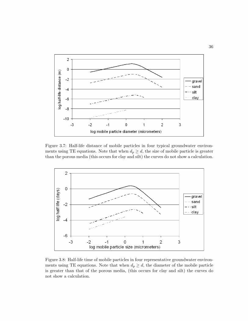
3.7 Half-life distance of mobile particles in four typical groundwater environ-

ments using TE equations. . . . . . . . . . . . . . . . . . . . . . . . . . . 36

3.8 Half-life time of mobile particles in four representative groundwater en-

vironments using TE equations. . . . . . . . . . . . . . . . . . . . . . . . 36

3.9 Half-life time of high- and low-density mobile particles in gravel aquifer. 38

3.10 Fraction of chemical removed from groundwater for 4 different aquifer

types. . . . . . . . . . . . . . . . . . . . . . . . . . . . . . . . . . . . . . 38

3.11 Travel of three chemicals in a gravel aquifer . . . . . . . . . . . . . . . . 39

3.12 Half-life distance of 5 particle types in run-off . . . . . . . . . . . . . . . 41

3.13 Half-life time of 5 particle types in run-off . . . . . . . . . . . . . . . . . 42

3.14 Half-life time of 3 particle types in run-off while varying rain and slope . 44

3.15 Half-lives of chemicals when sorbing to 5 different particles . . . . . . . 45

vii

3.16 Half-lives of chemicals when sorbing to a particle with two different focvalues . . . . . . . . . . . . . . . . . . . . . . . . . . . . . . . . . . . . . 45

3.17 Half-lives of chemicals when sorbing to two different particles with two

different foc values . . . . . . . . . . . . . . . . . . . . . . . . . . . . . . 47

4.1 Half-lives of high-density particles in 3 water compartments . . . . . . . 50

4.2 Half-lives of low-density particles in 3 water compartments . . . . . . . . 51

4.3 Half-lives of chemicals in 3 water compartments . . . . . . . . . . . . . . 53

4.4 A 3-D representation of particle and chemical removal in surface water . 55

viii

Chapter 1

Introduction

Production of food and fiber for use by people is a vital necessity, yet a highly con-

troversial one. The rise of modern agriculture, culminating in the Green Revolution

in the mid-20th century, has greatly increased the yield of crops [36]. In the last cen-

tury, yields were increased due to the use of fertilizers and pesticides, improved farm

machinery, development of hybrid strains, increase in irrigation, and changes in farm

management practices. The benefit of increased production, however, comes at the cost

of environmental degradation. The intensified use of land leads to erosion of soil which,

along with mobilized pesticides and fertilizers, contaminate both surface waters and

groundwater [38].

The negative results of the Green Revolution have illustrated that the focus of agri-

culture cannot be simply on productivity, but must also include sustainability [36] [15].

Given that chemical use and conventional methods of farming will never be completely

avoided, this desire for sustainability and environmental protection implies that, ”To

produce high yields, protect soil productivity, and maintain environmental quality, farm-

ing must be based on an understanding of how water and dissolved chemicals move

through the plant-soil-groundwater system” [38].

Water takes various forms on earth and is contained in different compartments.

The bulk of water resides in the ocean (96.5%), approximately 1.7% is in polar ice,

another 1.7% is stored as groundwater and the final 0.1% is contained in the atmosphere

and surface waters (streams, rivers, lakes, etc.) [7]. The circulation of water in the

atmosphere and on the earth’s surface is described by the hydrologic cycle. All parts

1

2

of the cycle occur simultaneously and the cycle is continuous with no beginning or

end. A starting point to describe the cycle is precipitation, which forms from water

that has evaporated from the land surface and the oceans. The precipitation then falls

back on the oceans and land. Precipitation enters groundwater through soil infiltration.

Groundwater moves through an aquifer (i.e. a porous media) and discharges to surface

waters (lakes, rivers, and streams). Precipitation also enters surface waters through

run-off from the land surface. Surface waters then discharge into the ocean where the

water is evaporated and again forms precipitation [7] [26].

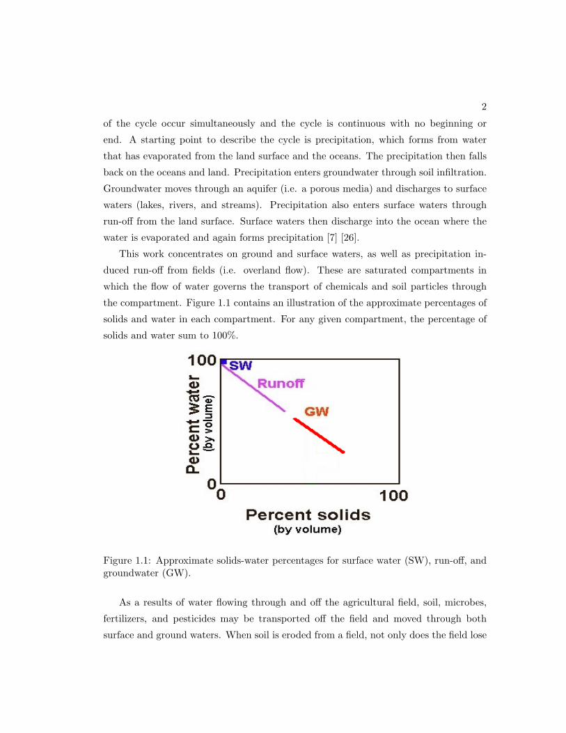
This work concentrates on ground and surface waters, as well as precipitation in-

duced run-off from fields (i.e. overland flow). These are saturated compartments in

which the flow of water governs the transport of chemicals and soil particles through

the compartment. Figure 1.1 contains an illustration of the approximate percentages of

solids and water in each compartment. For any given compartment, the percentage of

solids and water sum to 100%.

Figure 1.1: Approximate solids-water percentages for surface water (SW), run-off, andgroundwater (GW).

As a results of water flowing through and off the agricultural field, soil, microbes,

fertilizers, and pesticides may be transported off the field and moved through both

surface and ground waters. When soil is eroded from a field, not only does the field lose

3

beneficial topsoil, but the eroded soil can clog surface waters, destroy habitat, and impair

drinking water supplies [38] [34]. The micro-organisms in manure, which is applied as

fertilizer to many agricultural fields, are also a potential source of contamination to the

agricultural aquatic environment [24].

When chemicals leave the field, they can be both attached to soil particles and dis-

solved in the water. Therefore, an important concept related to fertilizers and pesticides

is that of sorption. Chemicals such as fertilizers and pesticides can be distributed among

three phases: water, solids, and air. When a chemical is introduced into the water, it

can become dissolved, sorb to the solids in the water, or volatilize to the air. For a given

chemical, all three phases can co-exist at the same time: one is not necessarily exclusive

of the other two. The distribution of a chemical amongst the three phases is a function

not only of chemical properties (e.g. water solubility, vapor pressure) and phase prop-

erties (e.g. temperature, organic carbon content), but also the relative volumes of the

three phases [27]. This paper does not cover volatilization, but instead focuses on the

dissolved (liquid) and sorbed (solid) phases and the transfer of chemicals between these

two phases.

One type of agricultural chemical that might be transported off the field is fertilizer.

This potential contaminant contains three important elements. The first, nitrogen,

exists in numerous chemical species (nitrate, ammonia, etc.). Nitrate is a frequent water

contaminant since it does not readily sorb to soil particles, leaches into groundwater, and

can impair the source water that is used for drinking water. The second, phosphorus,

strongly sorbs to soil particles. It can be carried to surface waters where it may cause

overgrowth of algae and other plants (eutrophication) which can lead to fish kills. The

third element included in fertilizer is potassium, but this is not generally considered to

be a water quality concern [38].

Pesticides are another type of common agricultural chemical. When pesticides leave

the field they have the potential of harming or killing aquatic and terrestrial organisms.

Some pesticides sorb readily to particles, while other, more soluble pesticides, tend to

stay in the dissolved phase and move through the environment with the water [38]. In

general, the main agricultural products, soil, fertilizers, pesticides, and micro-organisms,

are most useful and least harmful when contained to the agricultural field, but this is

very difficult to achieve due to water movement through and off the fields.

4

When soil, chemicals, or micro-organisms are transported off the field and enter the

water, they are often categorized by size. The larger constituents, such as sand, silt,

and clay which do not pass through a filter with 0.45 µm openings, are operationally

referred to as ”particulate” [12]. There is a group of constituents, such as small bacteria,

viruses, and colloids, however, which pass through a 0.45 µm filter, but can behave in

many ways similar to the larger particles. For the purposes of this paper, sand, silt, clay,

algae, bacteria, viruses, colloids, and similar constituents are referred to as ”particles”.

The constituents which can pass through a filter with 0.45 µm openings, such as

fertilizers, pesticides, and anions, are operationally defined as ”dissolved”. [12]. One

property of these chemicals, however, is that not only can they be truly dissolved, but

they can also be sorbed to particles that subsequently do not pass through the 0.45

µm filter. Chemicals dissolved in liquid are referred to as being ”dissolved” whereas

chemicals sorbed to particles are referred to as ”sorbed”.

Once particles and chemicals have been removed from the agricultural field into

surface water or groundwater, or as they are in the process of being removed from the

field such as in run-off, different mechanisms are at work in removing the constituent

from the water. In all three environments, sorption is an important mechanism by

which chemicals are removed [20]. In both surface water and run-off the chemicals sorb

to particles suspended in the water. A primary removal mechanism of these particles

is sedimentation [27]. In groundwater, assumed here to be a saturated porous media,

both chemicals and particles sorb to the media itself [42]. Additionally, particles in the

groundwater can be removed from the water via sieving or filtration [39]. Other removal

mechanisms for chemicals in the three water compartments are chemical reaction or

biological transformation [27]. The removal of chemicals by degradation or reaction,

however, is not addressed in this work.

There are many approaches used to model the removal and eventual fate of chem-

icals and particles in the three aquatic compartments considered here, surface water,

groundwater, and run-off. Some of these models are discussed in a review by Schulz

and Matthies [19]. These models can cover small or large scales in both space and time.

Some are designed for water and soil run-off during a single storm event (eg. KINEROS)

and can be applied on either a field-scale or watershed basis. Other models (eg. WEPP)

are intended for the watershed scale on a continuous, long-term time scale. A number

5

of models are designed to model leaching and infiltration of chemicals into groundwa-

ter (eg. GLEAMS) and transportation through groundwater (eg. STANMOD). These

models generally give reasonable and realistic results, but according to the review they

do lack accuracy in some situations (eg. high water flow, fate of pesticides or other

agricultural chemicals [19]).

Because of the large number of approaches used to model the removal of chemicals

and particles from various water bodies, a common expression would be helpful. The

holistic approach presented here introduces a new expression, a half-life of removal. This

term represents a standard quantification of the residence time of a chemical or particle

in a given water compartment. More specifically, the half-life is the length of time that

it takes for half of a given mass of constituent (particle or chemical) in a certain aquatic

environment to be removed from that water.

This common expression provides a unified approach and a common vocabulary with

which to talk about removal of particles and chemicals in different water compartments.

The half-life measure is versatile in that it can be calculated for any particle or chemical

in any aquatic environment for any removal mechanism. The half-life measure is also

universal in that the fate of a given particle or chemical can be compared against any

other chemical or particle for many different situations. The half-life could be found

in field experiments, but this work uses equations and models to compute a half-life of

removal for particles and chemicals in surface water, groundwater, and run-off.

Chapter 2

Methods

All of the models and equations presented in this chapter are utilized to produce a

common expression for removal of particles and chemicals from water. This versatile

expression is referred to as the half-life of removal, t1/2. This half-life term is not limited

to a chemical or biological reaction of the chemicals and particles in the water. Instead,

it represents a standard quantification of chemical and particle residence times in a

given aquatic environment. The half-life of removal is thus the length of time that

it takes for half of a given mass of the constituent (chemical or particle) in a certain

aquatic environment to be removed from that water. A half-life is used here (50%

removal) because of the existing half-life used for biological and chemical degradation

or reaction. The techniques and models presented here could also be used to calculate

the time at which 10% or 90% of a constituent was removed from the water.

Many different mechanisms contribute to the removal of particles and chemicals from

water. A few of these mechanisms are sorption, sedimentation, diffusion, interception,

filtration, degradation, and volatilization. The half-life of removal can encompass all

of these mechanisms. The half-life provides a method with which to discuss removal

with a common vocabulary rather than simply discussing how long it takes a chemical

to be removed from a water body through volatilization or how long it takes for a

particle to be removed via sedimentation. These removal mechanisms are represented

mathematically in various equations and models which can be utilized to calculate a

half-life of removal.

There are a number of environmentally simplified equations used here. The first set

6

7

of equations presented are those for sorption of chemicals. The next set of equations

are for sedimentation of particles and sedimentation of chemicals sorbed to particles

in surface water (SW). For groundwater (GW), equations are presented for modelling

the removal of particles by the processes of sieving, filtration, and sedimentation. The

behaviour of chemicals in groundwater is found using the STANMOD model [32] along

with a few equations for sorption. Removal of particles and chemicals in surface run-off

(RO) is calculated with the sediment transport model KINEROS along with the concept

of sorption [30].

A first-order removal rate is assumed so the general equation for concentration is

C = C0e−kt where C is the concentration at time t, C0 is the initial concentration and

k is the coefficient for rate of removal [13]. A list of all variables used in the equations

is contained in Appendix C. Although there exist highly detailed models which account

for many removal mechanisms, all of the equations and models used here to generate

half-lives are environmentally simplified. This is done in order to develop the half-life

concept rather than find the most realistic half-life. In utilizing these models, the aim is

not to find the exact half-life for every particle or chemical in a given situation. Rather,

the goal is to present a versatile new method of looking at particle and chemical removal

from a given water body.

2.1 Sorption

Sorption is an important mechanism by which chemicals are removed from water. Chem-

icals that are in water have different levels of solubility and different tendencies to either

remain dissolved in the water or to enter the particulate phase by associating with solids

that are in the water. The equilibrium constant that describes the extent of sorption is

Kd, the distribution coefficient, calculated using the equation

Kd =concentration of chemical associated with solid

concentration of chemical dissolved=

mass of chemical associated with solidsmass of solids

mass of chemical in aqueous phasevolume of water

(2.1)

This value is generally determined by laboratory experiments resulting in a sorption

isotherm. Because of the low concentration of chemicals active in the environment,

chemical behaviour in the linear portion of the Freundlich isotherm is almost always

8

observed [27]. Once the value of Kd is established, the fraction of the chemical sorbed

to particles in the water, fp, which is unit-less, can be calculated using Equation 2.2

fp =Kd[SS]

1 +Kd[SS](2.2)

where Kd is defined above and [SS] is the suspended solids concentration in water [41].

Another term that is utilized for sorption is Koc which is the distribution coefficient of

a chemical accounting for the fraction of organic carbon on the particle, foc, with units

of g carbong solid [1]. The relationship between Kd and Koc is

Kd = Koc ∗ foc (2.3)

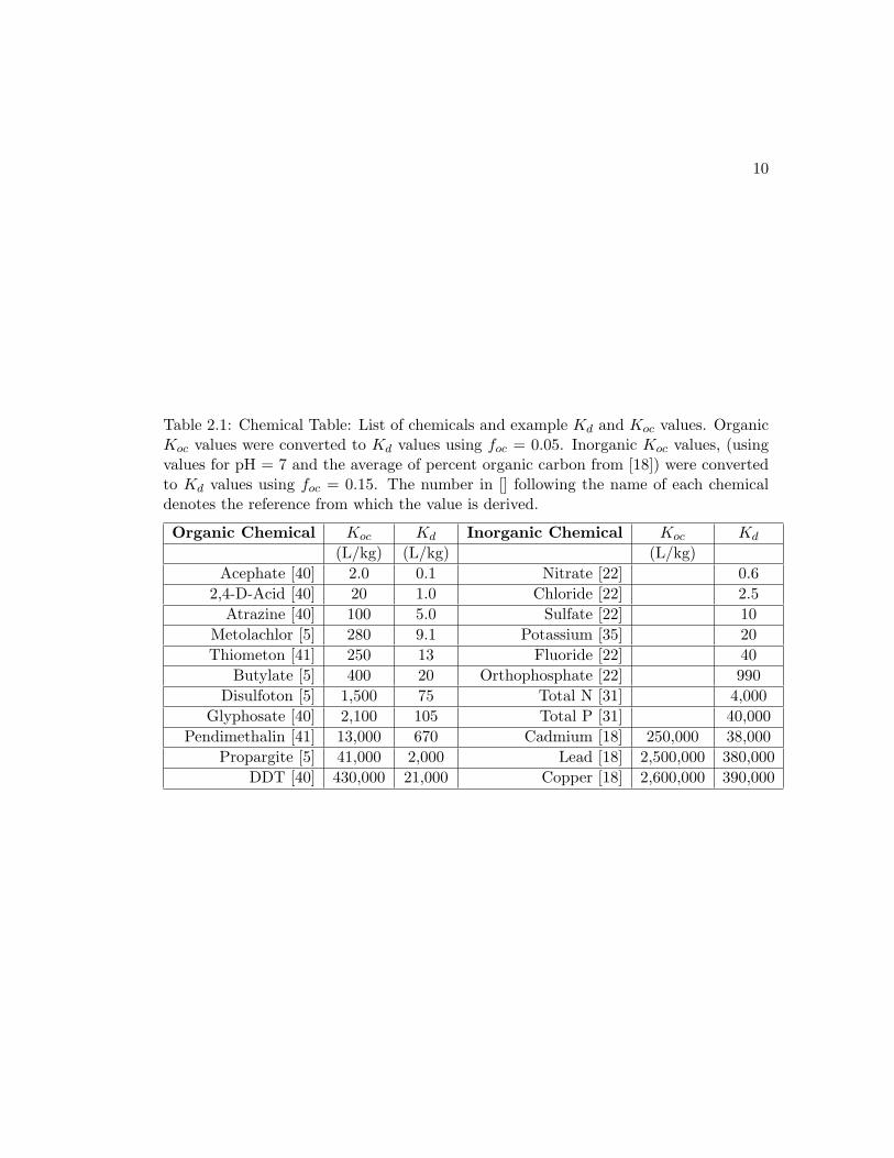
Table 2.1 contains a number of different chemicals and a value of Kd or Koc from the

literature.

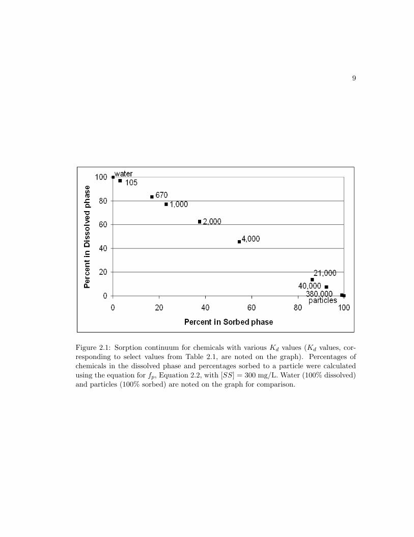
There is a large difference in the distribution coefficient of many chemicals, up to

a six orders of magnitude (in Kd values). Because of these distribution differences, the

extent of sorption of the chemicals varies greatly. All chemicals fall on a continuum

between 0% sorption (no chemical sorbed to solids, all chemical dissolved in water) and

100% sorption (all of the chemical sorbed to a particle, none dissolved in the water).

For a given aquatic environment, chemicals that are low on the sorption continuum (eg.

Kd < 102) are predominantly in the dissolved phase. Chemicals that have a larger Kd

value (eg. Kd > 102) tend to sorb to solids and can be removed from the water column

by sieving or settling of the associated particles. Figure 2.1 illustrates the sorptive

tendencies of chemicals with various Kd values, as noted on the figure. As a reference

point, water and particles are included, as well. Water can be thought of as being 0%

sorbed, 100% dissolved whereas particles are 100% sorbed, 0% dissolved.

9

Figure 2.1: Sorption continuum for chemicals with various Kd values (Kd values, cor-responding to select values from Table 2.1, are noted on the graph). Percentages ofchemicals in the dissolved phase and percentages sorbed to a particle were calculatedusing the equation for fp, Equation 2.2, with [SS] = 300 mg/L. Water (100% dissolved)and particles (100% sorbed) are noted on the graph for comparison.

10

Table 2.1: Chemical Table: List of chemicals and example Kd and Koc values. OrganicKoc values were converted to Kd values using foc = 0.05. Inorganic Koc values, (usingvalues for pH = 7 and the average of percent organic carbon from [18]) were convertedto Kd values using foc = 0.15. The number in [] following the name of each chemicaldenotes the reference from which the value is derived.

Organic Chemical Koc Kd Inorganic Chemical Koc Kd

(L/kg) (L/kg) (L/kg)Acephate [40] 2.0 0.1 Nitrate [22] 0.6

2,4-D-Acid [40] 20 1.0 Chloride [22] 2.5Atrazine [40] 100 5.0 Sulfate [22] 10

Metolachlor [5] 280 9.1 Potassium [35] 20Thiometon [41] 250 13 Fluoride [22] 40

Butylate [5] 400 20 Orthophosphate [22] 990Disulfoton [5] 1,500 75 Total N [31] 4,000

Glyphosate [40] 2,100 105 Total P [31] 40,000Pendimethalin [41] 13,000 670 Cadmium [18] 250,000 38,000

Propargite [5] 41,000 2,000 Lead [18] 2,500,000 380,000DDT [40] 430,000 21,000 Copper [18] 2,600,000 390,000

11

2.2 Surface Water

There are two equations used here to calculate the half-life of removal of particles and

chemicals in surface water. The first is the removal of particles from the water by

sedimentation and the second is sorption of chemicals to particles and their subsequent

sedimentation. A number of simplifying assumptions are made about the surface water

system before the equations are presented. Typical values for the variables follow the

equations.

2.2.1 Assumptions

The system or control volume used here is a given section of stream, river, or lake.

The upstream flow is the source of the inputs and both the downstream flow and the

sedimentation of chemicals and particles to the bed are the outputs. The water is

assumed to have uniform laminar flow with no turbulence and no longitudinal dispersion.

Other assumptions being made are that the system is at sorptive equilibrium, there is a

constant settling velocity for particles of a given size and density, and there is a constant

input concentration of particles and chemicals from upstream. The final assumptions are

that no chemicals or particles are stored in the water column inside of the control volume,

and there are no chemicals or particles removed through degradation or volatilization

processes. Because the results in Chapter 3 do not include any fluid dynamics such as

advection, turbulence, or dispersion, the half-lives of removal are identical to those that

would be computed for an immobile column of water. For this reason, the half-lives can

be applied to all surface waters, including lakes, rivers, and streams.

2.2.2 Particle Removal

The movement of water in lakes or rivers has profound influence on particle behaviour.

Detailed hydrodynamic models accounting for advection, dispersion, turbulence, etc. are

available citeRefWorks:18, however, they are not used here. Based on the assumptions,

particle removal in surface waters is a function of sedimentation, with an equation for

the kinetic rate constant for sedimentation being

ksed =vsh

(2.4)

12

where vs is the velocity of sedimentation for a certain type of particle and h is the depth

of the water body [41]. This rate constant, ksed, takes the place of the rate constant k in

the equation for concentration, C = C0e−kt. Different particles have different settling

velocities, vs. Table 2.2 contains a list of selected particles and their typical settling

velocities. These values are used with the assumption that these setting velocities are

typical of a no-turbulence situation. The Stoke’s settling velocities in Table 2.2 are

calculated using Equation 2.5

vt =gd2(ρp − ρw)

18µ(2.5)

where g is acceleration due to gravity, d = diameter of the particle, ρ = density of

particle, p, or water, w, and µ is the viscosity of water [17].

The half-life of a particle in water, t 12, can be obtained by solving the equation

C = C0e−ksedt to find where concentration at time t 1

2is half of the initial concentration.

The variable C represents the total concentration of the given particle. The equation

for the half-life of removal of a given particle is Equation 2.6 [41].

t 12

= ln(2)ksed = ln(2)h

vs. (2.6)

2.2.3 Chemical Removal

Chemical removal in surface waters is a combination of sorption and sedimentation,

which combines Equation 2.2, fraction of the chemical associated with the particle, and

Equation 2.4, the rate of sedimentation. The combined equation is

ksed =vshfp (2.7)

The equation for half-life of the chemical is identical to that of particles. The only dif-

ference is that, fp = 1 for particles because there is no need to account for sorption [41].

t 12

= ln(2)h

vsfp. (2.8)

2.2.4 Typical Values for Equation Parameters

In the environment, a range of values is possible for each of the parameters in the

equations for sorption and sedimentation. Values that are used for [SS] in Equation 2.2

are 3, 10, 30, 100, 300, and 1000 mgL . The values for Kd range from Kd = 0.1 (log

13

Kd = -1) to Kd = 10,000,000 (log Kd = 7) Lkg which is approximately the range of Kd

values in Table 2.1. The remaining variable that is necessary for Equation 2.7 is depth,

h. Values used for h are 0.1, 0.3, 1, 3, and 10 m. These values are representative of

a range of surface waters from a very shallow stream to a relatively deep river. The

foc values range from 0.01, for particles such as sand with low organic content to foc

= 0.4 for particles such as algae with a high organic content. Table 2.3 contains a

list of the six example particles that are followed in the particle computations. These

particles represent a wide range of particles that may exist in the environment. The

settling velocities of these particles were calculated using Stoke’s Equation, 2.5, and

the accompanying constants.

14

Table 2.2: Particle Table: List of particles (µm) along with the calculated Stoke’ssettling velocity (m/s) and settling velocities from literature (m/s). Stoke’s velocitieswere calculated using the given densities, g = 9.81m/s2, the given diameters, ρw = 998.2mg/m3 and µ = 0.001002 kg/(m ∗ s), where both density and viscosity are of water at20 ◦C. Stoke’s velocity is calculated using Equation 2.5.

Particle Size Range or Typical Stoke’s vs LiteratureType Typical Diameter (µm) Density ( kg

m3 ) Range (m/s) vs (m/s)Sand 2,000 to 62.5 [16] 2650 [16] 3.6 to 0.004 0.02 [21]

Silt 62.5 to 2 [16] 2650 [16] 0.004 to 0.000004 0.002 [21]Clay less than 2 [16] 2650 [16] less than 0.000004 0.00002 [21]

Flocs 6.8 [9] 1040 [9] 0.0001 0.0015 [9]Algae 10 [4] 1001 0.0000002 0.01 [6]

Bacteria 5 [4] 1001 0.00000004 0.0001 [2]Virus 0.1 [28] 1085 [28] 0.0000000004 -

Table 2.3: Settling velocities (m/s) for particles of various diameters and densities.Diameters are listed in the table. The column ”hd vs” (high-density vs) contains settlingvelocities for particles with densities of 2650 kg/m3 whereas the column ”ld vs” (lowdensity vs) contains settling velocities for particles with densities of 1085 kg/m3.

Particle diameter hd vs ld vsname (µm) m/s m/ssand-sized 200 0.036 0.0018silt-sized 60 0.0032 0.00017clay-sized 2 0.0000036 0.00000019

15

2.3 Groundwater

The equations and assumptions for particle and chemical removal in groundwater are

quite different from each other. Particle removal is accomplished by sieving or filtration.

Chemical removal occurs by sorption to both particles in the water and to the porous

media itself. A number of simplifying assumptions are made about the groundwater

system before the equations are presented. Typical values for the variables follow the

equations.

2.3.1 Assumptions

For both the particle and chemical removal in groundwater, there are a number of

simplifying assumptions present. First of all, the system or control volume used here

is a given 1-D length of aquifer composed of spheres of uniform diameter (the porous

media). The up-gradient water flow, which is constant, is the source of the inputs and

the down gradient flow is an output. The other output for chemicals and particles is

removal by the porous media (via sorption, sieving, etc). The water flow is assumed to

have no longitudinal dispersion. Other assumptions being made are that the chemical

system reaches sorptive equilibrium immediately and that there is permanent storage of

the removed particles on the aquifer medium. There is a constant input concentration of

particles and chemicals from up-gradient. There are no chemicals or particles removed

through degradation processes. Finally, the assumption is made that particle removal

causes no head loss or overloading of the stationary solids, since groundwater typically

has a low suspended solids concentration.


The basis for modelling mobile particle removal in groundwater is the single-collector

efficiency equations, developed by Yao [43]. The single-collector is a sphere past which

the mobile particles flow. Many single-collectors with the same diameter together create

a porous media (i.e. aquifer). Tufenkji and Elimelech (TE equations) [39] adapted the

single-collector equations for use with the slow flow rates of groundwater (less than 10

m/d). The TE equations calculate the removal of mobile particles ranging in size from

0.01 to 100 µm. This accounts for particles as small as a virus or bacterium to those as

16

large as silt and small sand.

Under steady-state conditions, the equation used to calculate removal efficiency in

the aquifer is

ln(C

C0) =

−3L(1− ε)αη0

2d(2.9)

where ε is the porosity of the aquifer, L is the length of aquifer travelled, d is the diameter

of the porous media, α is the attachment efficiency and η0 is the single-collector contact

efficiency which is defined below [29]. Using the overall removal efficiency of particles

in a filter, 1− CC0

[10], the equation for removal efficiency becomes the following.

1− C

C0= 1− e

−32dL(1−ε)αη0 (2.10)

where the equation for single-collector efficiency is

η0 = ηD + ηI + ηG (2.11)

The primary mechanisms for particle removal are diffusion, D interception, I, and grav-

ity, G. Diffusion describes when the mobile particles contact the porous media through

Brownian motion. Interception refers to when a mobile particle contacts the porous

media as it flows along a streamline. Mobile particles that have densities greater than

that of water contact the porous media through settling due to gravitational forces. The

TE equations for each of these mechanisms are defined below [39].

ηD = 2.4A1/3s N−0.081

R N−0.715Pe N−0.052

vdW (2.12)

ηI = 0.55AsN1.55R N−0.125

Pe N0.125vdW (2.13)

ηG = 0.22N−0.24R N1.11

G N0.053vdW (2.14)

The non-dimensional values NR, aspect ratio, NPe, Peclet number, Nvdw, van der Waals

ratio, NG, gravitational number, As, porosity-dependent parameter, and D∞, diffusion

coefficient, are

NR =dpd

(2.15)

NPe =vd

D∞(2.16)

NvdW =A

kT(2.17)

17

NG =d2p(ρp − ρw)g

18µv(2.18)

D∞ =kT

3πµdp(2.19)

As =2(1− γ5)

2− 3γ + 3γ5 − 2γ6(2.20)

γ = (1− ε)1/3 (2.21)

and the variables are defined as follows.

ε = porosity

α = empirical collision (attachment) efficiency

η0 = single collector contact efficiency

d = grain size of filter media

dp = diameter of suspended particles

L = bed depth, distance travelled

ηD, ηI , ηG = single collector contact efficiency for diffusion, interception, sedimentation, re-

spectively

k = Boltzmann constant

T = absolute temperature

µ = water viscosity

ρp, ρw = density of particles and water

g = gravity constant

v = water velocity

A = Haymaker constant

18

Given that an equation for half-life is desired (the point in time or space where CC0

= 12

Equation 2.10 simplifies to12

= e−32

(1−ε)αη(Ld

) (2.22)

The half-life can then be found in terms of a distance travelled, a half-life in distance

L1/2 =2ln(2)d

3(1− ε)αη0(2.23)

or in terms of time, by substituting in L1/2 = vt1/2 so that the equation for a half-life

in time is as follows.

t1/2 =2ln(2)d

3(1− ε)αη0v. (2.24)


The half-life of removal for chemicals is easy to compute given the simplifying assump-

tions present. It can be shown (see Appendix B) that the fraction of the chemical, fp,

Equation 2.2, can be re-written as

fp = 1− 1R

(2.25)

where the retardation coefficient, R, is defined as

R = 1 +ρbKd

ε(2.26)

and ρb is the dry bulk density of the porous media, Kd is the distribution coefficient for

a given chemical, and ε is the porosity of the porous media. Using Equation 2.25, the

half-life of removal occurs when fp = 12 which is where R = 2, or 1 = ρbKd

ε . Also, by

assuming that there is no dispersion, the location of the chemical can be calculated by

another equation for R,

R =vwvc

=velocity of groundwatervelocity of contaminant

(2.27)

so for a chosen time, t, the equation for distance travelled, d, is

d =tvwR

(2.28)

where vc = dt .

19

In order to generate graphs of the chemical transport, the software program STAN-

MOD [32] is used. STANMOD utilizes analytical solutions to the convection-dispersion

solute transport equation in order to calculate solute transport in a porous media [33].

Dispersion, D, is set to a negligible amount, 10−8, to follow the assumption of no dis-

persion. The sub-program of STANMOD used here is the CXTFIT module. In the

pre-processing menus, the following options are used:

• Type of Problem: Direct problem. Number of parameter sets varies.

• Model Code: Deterministic equilibrium CDE.

• Input and Output Data Code: Time and position are dimensional.

• Time and space units: Length, m. Time, days. Concentration, dimensionless

• Concentration mode: Resident concentration (third-type inlet), Cr.

• Transport and reaction parameters: v, varies for each aquifer type. D = 10−8. R,

varies by both aquifer type and Kd value. µ = 0, where µ is an internal STANMOD

degradataion coefficient.

• Boundary value problem: Pulse input at application time T. Input concentration

= 1, Application time = 1.

• Initial value problem: Zero initial concentration.

• Production value problem: Zero production.

• Output structure: Varies upon desired output.

The generated graphs illustrate the distances that the chemicals travel in different

aquifers. By computing the integral under the curves of concentration, a calculation

performed by STANMOD, the total mass of chemical dissolved in the water can be

found.

2.3.4 Typical Values Used

For particle removal, the values used for constants in the TE equations are as follows.

20

dp = diameter of mobile particles, 10−2 µm to 102 µm

L = distance travelled, variable

k = Boltzmann constant = 1.380662 ∗ 10−23J/K

α = empirical collision (attachment) efficiency = 0.05

T = absolute temperature = 283K = 10 ◦C

µ = water viscosity at 10 ◦C = 0.001308 kgms

ρp, ρw = density of particles and water at 10 ◦C = 2650 or 1085 for particles and 999.7kgm3 for water

g = gravity constant = 9.81 ms2

A =Hamaker constant = 2 ∗ 10−20 J .

The other parameters are varied in representative aquifers for illustrative purposes in

both the TE equations and STANMOD. The representative aquifer media and their

assumed particle diameters, d, porosities, ε, flow rates,v, and bulk densities, ρb are

given in Table 2.4.

Table 2.4: Representative aquifer media and their assumed particle diameter, d, poros-ity, ε, groundwater flow rate,v, and bulk density, ρb, as used in the TE model andSTANMOD. References and calculations are found in Appendix A

Aquifer type diameter, d porosity, ε velocity, v bulk density, ρbmm µm – m/d kg/L

Gravel 10 104 0.20 5 1.8Sand 1 103 0.25 0.4 1.65

Silt 0.01 10 0.40 0.0025 1.35Clay 0.001 1 0.50 0.00002 1.2

21

2.4 Surface Runoff

The analysis of particle behaviour in run-off is done using the sediment transport model

KINEROS [30]. The chemical removal is analyzed using the equation for sorption, Equa-

tion 2.2, combined with data from KINEROS. A number of simplifying assumptions are

made about the run-off system before the equations are presented. Typical values for

the various equation variables follow the equations and program information.

2.4.1 Assumptions

As in the surface water and groundwater analysis, a number of simplifying assumptions

are made. The control volume used here is a given mass of sediment in a constant volume

of water which forms run-off (overland flow) on a given hillside with no vegetation. Input

flow to the control volume is not constant since the flow varies by storm events and flow

is not constant during a storm event. Output of particles and chemicals occurs via

deposition onto the soil surface and by exit off the field. This system is also assumed

to be at sorptive equilibrium, which occurs quickly compared to sediment transport

processes [37]. It is assumed that chemicals are only removed from the run-off water

via sorption to mobile particles and the subsequent deposition of those particles. There

is no removal of particles or chemicals via degradation or volatilization.


Particle removal in run-off is modelled using the sediment transport model KINEROS [30].

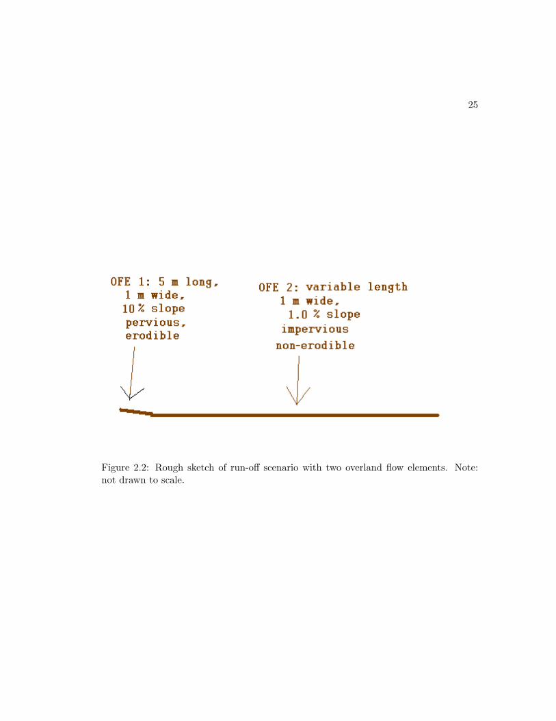
A single storm event with two overland flow elements (OFEs) is modelled using the sce-

nario pictured in Figure 2.2. A heavy rain generates run-off on OFE 1, which is a 5 m

long, 1 m wide, pervious, erodible surface with slope of 10%. There are two soil layers

on this element, the top layer is porous and erodible (and generates the particles in

the run-off) whereas the lower layer is impervious (to avoid loss of water). The run-off

(including water, chemicals, and particles) is subsequently routed to OFE 2, a variable

length, 1 m wide, impervious, non-erodible surface with slope of 1.0%. Any remaining

run-off is routed off the end of OFE 2. The length of OFE 2 is varied in order to find

the half-life of removal of various particle types. Rain is simulated on both OFE 1 and

OFE 2 at a rate of 2 mm/min for a total of 6 mm in 3 minutes.

22

The two field elements are assumed to be impervious so that the computation of

half-life is simplified. An impervious surface implies that the water in the active run-off

flow remains constant. This enables the half-life to computed from the mass, M, of

sediment instead of the concentration, C, of suspended solids in the water. In terms of

equations, the general equation for concentration is C = C0e−kt where C = M/V and

CO = M0/V0. Using the fact that V = V0, from the assumption of impervious surfaces,

this can simplify to M = M0e−kt.

The model KINEROS is used to produce sediment output data at a user-specified

time and/or a user-specified location. A time step of 0.1 minutes (6 seconds) is used here

and the simulation is run for a total of 2000 minutes. The model is used to calculate the

movement of five particle types: high-density (2650 kg/m3) sand-, silt-, and clay-sized

particles and low-density (1085 kg/m3) silt-, and clay-sized particles. At each time step,

the output generated by KINEROS is both the amount of water flowing past a certain

location on the field (in units of m3/s) and the amount of sediment flowing past that

point (in units of kg/s). At the end of OFE 1, the only sediment-producing section of

the field, the total mass exiting the field element is calculated for each particle, M0,p

for a given particle type, p. Then, for various distances, d, on OFE 2, the total mass of

each particle type passing that point is calculated, Md,p. The fraction of particle type,

p, remaining at any given distance, d, on the field is thus Md,p

M0,p. When this fraction

goes below 12 , then half of that certain particle type has been deposited at or before the

distance, d. The half-life in time is then obtained by examining the sediment time-scale

output data to find when the output of the sediment type reached 0 kg/s. This is

necessary due to the fact that some particles types may settle by the same distance (eg.

15 meters) but by different times (10 minutes for high-density silt-sized particles versus

25 minutes for low-density silt-sized particles).


Given the simplifying assumptions made, the half-lives of chemicals in surface run-off

are calculated using the equation

t 12,c =

t 12,p

fp(2.29)

23

where t 12,c is the half-life of a given chemical, c, t 1

2,p is the half-life of the particle, p,

that the chemical sorbs to, and fp is the fraction of the chemical that is sorbed to the

given particle. The half-life, therefore, not only depends on the type of particle present,

but also upon the foc of that particle and the [SS] of the run-off. The variables foc and

[SS] are utilized in the equations for Kd (2.3) and fp (2.2), respectively.

2.4.4 Typical Values Used

The soil present in the top layer of OFE 1 includes high-density (2650 kg/m3) sand-,

silt-, and clay-sized particles with diameters of 200, 60, and 2 µm, respectively. The soil

also includes low-density particles (1085 kg/m3) of the smaller diameters, 60 and 2 µm.

These are the same sizes and densities of particles used in the surface water section and

the same densities used in groundwater. The particle class fractions in the initial top

layer of soil are initially equal (each fraction is 20%). The top layer of soil on OFE 1

has a 0.5 m thickness while the lower layer is impervious. Other parameters used in the

program are as follows:

• Temperature = 20 ◦C

• Slope of OFE 1 = 10 %

• Length of OFE 1 = 5 meters

• Manning roughness coefficient, OFE 1 = 0.05, typical of fallow soil [30]

• Initial saturation of soil, OFE 1 = 0.2

• Saturated hydraulic conductivity (Ks) of upper soil, OFE 1 = 10 mm/hr, typical

of semi-pervious soil made up of sand, silt, and clay [3]

• Pore size distribution index, upper soil, OFE 1 = 0.4

• Porosity, upper soil, OFE 1 = 0.35

• Rainsplash coefficient, upper soil, OFE 1 = 50

• Soil cohesion coefficient, upper soil, OFE 1 = 0.5

• Slope of OFE 2 = 1.5%

24

• Length of OFE 2 = variable

• Manning roughness coefficientor, OFE 2 = 0.011, typical of concrete or asphalt [30]

• Fraction of surface covered by erosion pavement, OFE 2 = 1

The equations for chemical removal in run-off use half-life time results derived from

the KINEROS data. One variable that is utilized for chemical removal is that of foc.

As in the surface water section, the computations for chemical removal in run-off use

foc = 0.01 and foc = 0.4. Also for the chemical calculations, the [SS] is assumed to be

30,000 mg/L which is 1000 times greater than the [SS] in surface water. This value is

approximately the [SS] exiting OFE 1. It is found by dividing the total sediment that

exited OFE 1 (kg) by the total volume of water that exited OFE 1 (L).

25

Figure 2.2: Rough sketch of run-off scenario with two overland flow elements. Note:not drawn to scale.

Chapter 3

Results

A brief examination of sorption and the variables influencing it is at the beginning of

this chapter. This is followed by sections pertaining to particle and chemical removal

in surface water, groundwater, and run-off. The versatility of the half-life measure is

demonstrated in these sections by not only computing half-lives of particles as a function

of particle diameter but also computing half-lives of chemicals as a function of Kd values.

3.1 Sorption

The sorptive properties of various chemicals can be examined by looking at the rela-

tionship between Kd and fp using the six values for [SS], a range of values for Kd, and

Equation 2.2. Figure 3.1 illustrates that as log Kd increases, the fraction of the chemical

associated with the particle increases from about 0% for chemicals like nitrate and chlo-

rine, which have very low Kd values, to 100% for metals such as lead and copper, which

have very high Kd values (see Table 2.1). The curves for the different suspended solids

values have similar shape, but the curves show that with a higher [SS] concentration,

there is a greater fp, fraction of the chemical associated with the particle. For example,

Total P has log Kd = 4.6 so if [SS] = 3 mg/L, fp is 11%, but if [SS] = 1000 mg/L, fpis 98%.

For many organic chemicals, another factor that influences fp is foc. The organic

content of the paricles, foc indirectly influences fp via the relationship between Kd and

26

27

Figure 3.1: Fraction of the chemical associated with the particle (fp), depending on Kd

value, varying [SS], using Equation 2.2.

28

Koc. The equation for converting Koc to Kd is Kd = Koc ∗ fp so by substituting this

into Equation 2.2, the equation for fp becomes

fp =Kocfoc[SS]

1 +Kocfoc[SS](3.1)

Three different foc values are considered in this equation: foc = 0.01, 0.1, 0.4, repre-

senting low, medium, and high organic content. The lines for the three foc values in

Figure 3.2 follow the same curve because the [SS] for each is the same. The points on

the graph, however, illustrate the effect of foc when converting the Koc value to Kd.

The points represent the fraction of the chemical sorbing to the particle, fp, for DDT

when sorbing to particles with different foc values. When foc = 0.01, the fp for DDT is

11%, however, when foc = 0.4, fp for DDT increases to 84%.

Figure 3.2: Fraction of the chemical associated with the particle (fp), as a function ofthe Kd value for various chemicals. The points on the graph represent DDT sorbing toparticles with foc=0.01, 0.1, and 0.4.

29

3.2 Surface Water

Particle removal in surface water is influenced not only by height of the water body,

but also by the settling velocity of the particles, as can be seen from Equation 2.6.

The change in half-life is examined for water bodies of different heights, followed by an

examination of how particle density influences half-life, via the settling velocity.

Chemical removal in surface water is influenced by [SS] and foc, in addition to the

variables that affect particle removal, height and settling velocity. The chemical removal

section focuses only on the half-lives of high-density particles with varying foc values.

This is due to the fact that [SS] was examined in connection to sorption whereas height

and settling velocity are examined in connection with particles. Height is set to 3 m

and [SS] is kept at 30 mg/L.


In order to examine the half-lives of particles being removed from surface water, the

values generated from Equation 2.6 are presented in Figure 3.3. This graph displays

half-life, t1/2, as a function of particle diameter, d, and examines the influence of height

on removal half-life. As is logical, an increase in height produces the same magnitude

increase in half-life. The graph gives half-lives for particles of size 0 to 300 µm with

densities of 2650 kg/m3. As noted in Table 2.2, this range accounts for small sand, silt,

and clay. The larger particles (gravel and large sand) are omitted due to their rapid

settling and brief half-life in comparison to clay-sized particles.

A second graph for examining the half-life of particle removal in surface water,

Figure 3.4, shows a comparison of high- and low-density particles, with densities of

2650 and 1085 kg/m3, respectively. The graph shows that the half-life of particles

decreases when either the particle size increases or the density increases. Sand-, silt-, and

clay-sized particles for both densities are noted on the graph. There is approximately

one order of magnitude difference between same-sized particles with different densities.

30

Figure 3.3: Half-life of high-density particles (2650 kg/m3) with different diameters(ranging from clay- to sand-sized) in environments of different heights, using Equa-tion 2.6. Five different heights (in meters) are noted on the graph.

Figure 3.4: Half-life of particles with different diameters (ranging from clay- to sand-sized) and different densities (1085 and 2650 kg/m3), using Equation 2.6. Marked onthe graph are the specific half-lives of sand-, silt-, and clay-sized particles with respectivesizes of 200, 60, and 2 µm. Height is 3 m.

31


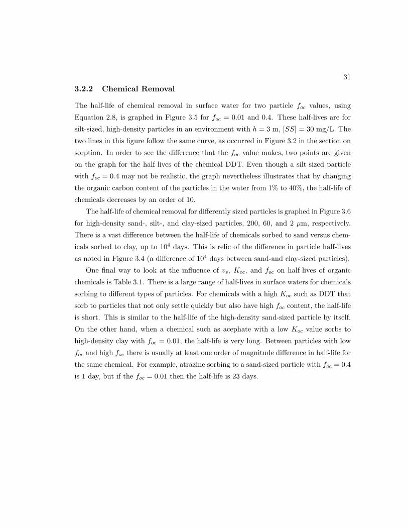
The half-life of chemical removal in surface water for two particle foc values, using

Equation 2.8, is graphed in Figure 3.5 for foc = 0.01 and 0.4. These half-lives are for

silt-sized, high-density particles in an environment with h = 3 m, [SS] = 30 mg/L. The

two lines in this figure follow the same curve, as occurred in Figure 3.2 in the section on

sorption. In order to see the difference that the foc value makes, two points are given

on the graph for the half-lives of the chemical DDT. Even though a silt-sized particle

with foc = 0.4 may not be realistic, the graph nevertheless illustrates that by changing

the organic carbon content of the particles in the water from 1% to 40%, the half-life of

chemicals decreases by an order of 10.

The half-life of chemical removal for differently sized particles is graphed in Figure 3.6

for high-density sand-, silt-, and clay-sized particles, 200, 60, and 2 µm, respectively.

There is a vast difference between the half-life of chemicals sorbed to sand versus chem-

icals sorbed to clay, up to 104 days. This is relic of the difference in particle half-lives

as noted in Figure 3.4 (a difference of 104 days between sand-and clay-sized particles).

One final way to look at the influence of vs, Koc, and foc on half-lives of organic

chemicals is Table 3.1. There is a large range of half-lives in surface waters for chemicals

sorbing to different types of particles. For chemicals with a high Koc such as DDT that

sorb to particles that not only settle quickly but also have high foc content, the half-life

is short. This is similar to the half-life of the high-density sand-sized particle by itself.

On the other hand, when a chemical such as acephate with a low Koc value sorbs to

high-density clay with foc = 0.01, the half-life is very long. Between particles with low

foc and high foc there is usually at least one order of magnitude difference in half-life for

the same chemical. For example, atrazine sorbing to a sand-sized particle with foc = 0.4

is 1 day, but if the foc = 0.01 then the half-life is 23 days.

32

Figure 3.5: Half-life of chemicals sorbing to particles with foc = 0.01 and 0.4, usingEquation 2.8. Values shown are for high-density, silt-sized particles with h = 3 m, [SS]= 30 mg/L.

Figure 3.6: Half-life of chemicals sorbing to sand-, silt-, and clay-sized particles, 200, 60,and 2 µm, respectively, using Equation 2.8. Values shown are for high-density particleswith h = 3 m, [SS] = 30 mg/L.

33

Table 3.1: Half-lives for 4 different chemicals sorbing to 2 different sized high-densityparticles with two different foc values, [SS] = 30 mg/L, h = 3 m. Half-lives are in years(y), days (d), and minutes (min). Half-lives of sand and clay particles themselves are1 minute and 7 days, respectively. Original Koc values for each chemical taken fromTable 2.1.

clay-sized clay-sized sand-sized sand-sizedChemical foc = 0.01 foc = 0.4 foc = 0.01 foc = 0.4Acephate 31,000 y 750 y 3 y 28 dAtrazine 600 y 15 y 23 d 1 d

Glyphosate 29 y 269 d 1 d 39 minDDT 58 d 8 d 8 min 1 min

34

3.3 Groundwater

Particle removal in groundwater is influenced not only by the size and density of the

mobile particles, but also by the properties of the porous media through which the water

flows. The change in half-life of particles is examined for four different types of porous

media followed by an examination of how particle density influences removal.

Chemical removal in groundwater is primarily influenced by the type of porous

media. The behaviour of chemicals with various Kd values is calculated for the four

representative aquifer types.


In order to examine how particles are removed from groundwater, the half-life of particles

can be found at either a point in time or a physical location, as demonstrated by

Equations 2.23 and 2.24. The values generated from the equation for the physical

location of the half-life of particles are presented in Figure 3.7. This figure shows that

the type of porous media has a substantial influence on the travel distance of particles.

Particles with a 1 µm diameter travel 1 meter in a gravel aquifer whereas those same

particles travel only 0.1 µm in a clay aquifer (or in reality never actually enter an aquifer

of clay since clay particles are approximately 1 µm). When the grain size of the porous

media is smaller than the diameter of the incoming particles (dp ≥ d), the curves are

not shown since realistically particles of this size would never enter a porous media with

smaller sized particles. This occurs for clay (d=1 µm) and silt (d = 10µm).

The half-life in terms of length of time the particles remain in groundwater, Equa-

tion 2.24, is given in Figure 3.8. The graph is very similar to the graph of half-life

distance, Figure 3.7 since the distances are simply scaled by the groundwater velocity

for each type of porous media in order to obtain a half-life in time. Both figures show

a longer half-life of removal for particles of size 1 µm than for either larger or smaller

particles. This occurs because sedimentation, diffusion, and interception, as represented

in the TE equations, affect the range of particle sizes in different ways. Diffusion is more

effective for particles of smaller size whereas interception and sedimentation affect the

larger particles more than the smaller ones. The combined influences of these three

processes of filtration are least effective near 1 µm which corresponds directly to the

35

location of the longest half-life of removal of particles in groundwater. This is also the

approximate size of most bacteria whereas most viruses are slightly smaller, with most

having a diameter less than 1 µm [25].

One final variable affecting particle removal in groundwater is that of particle density.

In surface water the density of the particle had a sizeable influence on the half-life and

particle density in groundwater is no different. Figure 3.9 shows half-lives of removal for

the two densities that were used in surface water: high-density (2650 kg/m3) and low

density (1085 kg/m3). It is interesting to note that in groundwater, the change in density

only affects the larger particles. This is due to the TE equations used in calculation.

Higher density particles have a shorter half-life, by a factor of ten, compared to the

lower density particles. This theoretical result is arguable given that the lower density

particles tend to be organisms that themselves are mobile. This fact could lead to less

of a difference between half-lives of low- and high-density particles [25].


Chemical removal in groundwater is examined by using the equation for fp in ground-

water, Equation 2.25, along with the equation for R, 2.26. These two equations yield

the result that 50% of the chemical mass is removed from the water in the aquifer when

1 = ρbKdε . Given the assumption that there is instantaneous sorption and desorption,

this equality implies that at any given time there is one Kd value for any given aquifer

for which 50% of the chemical is sorbed to the solids and 50% is dissolved in the water.

For this reason, no half-life in time is calculated for chemicals in groundwater. In real

life, these simplifying assumptions do not hold. This implies that not only is there

storage of the chemical on the aquifer medium, but also a half-life in time could be

computed. The theoretical exercise here is instructive, however, because it illustrates

the general tendencies of chemicals in groundwater.

Figure 3.10 gives a graph of the values generated by Equation 2.25. Recall that fp is

the fraction or percent of the chemical that is sorbed to the aquifer media. For a given

aquifer with constant values for both ε, porosity, and ρb, bulk density, the Kd value for

which there is 50% removal is simply Kd = ερb

. The Kd values for which there is 50%

sorbed, 50% dissolved for each aquifer type in Figure 3.10 are 0.11, 0.15, 0.3, or 0.42

L/kg for gravel, sand, silt, and clay respectively. Under the assumptions made, any Kd

36

Figure 3.7: Half-life distance of mobile particles in four typical groundwater environ-ments using TE equations. Note that when dp ≥ d, the size of mobile particle is greaterthan the porous media (this occurs for clay and silt) the curves do not show a calculation.

Figure 3.8: Half-life time of mobile particles in four representative groundwater environ-ments using TE equations. Note that when dp ≥ d, the diameter of the mobile particleis greater than that of the porous media, (this occurs for clay and silt) the curves donot show a calculation.

37

value below this results in less than 50% of the chemical being sorbed whereas any Kd

value above this yields greater than 50% sorbed.

In order to illustrate how chemicals with various Kd values travel, STANMOD is

used the generate a graph with three different Kd values in a gravel aquifer. The three

Kd values of 0, 0.11, and 0.33 correspond to R values of 1, 2, and 4, respectively. These

R values then represent 0% removal from the water (i.e. sorbed to media), 50% removal,

and 75% removal. In the figure, the chemical is input to the water for one day in a pulse

of 1 µg. In STANMOD this is implemented by dissolving 1 µg of chemical in the water

with the corresponding amount sorbed to the aquifer media, as determined by the Kd

value. Thus, because the groundwater velocity in the representative gravel aquifer is 5

m/d, there is a total of 5 µg input into the aquifer. It is interesting to note that not only

does the R value influence the velocity of the chemical, as given in Equation 2.27, but

the R value also influences the percent of the chemical which is removed. For example,

for an R value of 1 (Kd = 0), there is no removal of the chemical and by day 2 (one day

after the pulse input) the front of the pulse has travelled 10 meters (i.e. no retardation,

it travels at the same velocity as the water). For Kd = 0.11 (R = 2) the front of the

pulse has travelled 5 meters (half the distance the water has travelled) and there is only

2.5 µg dissolved in the water (half of the original mass). Similarly for Kd = 0.33 (R =

4), there is a 75% decrease in total dissolved mass (1.25 µg) and the front of the pulse

has travelled only 2.5 meters (75% of the distance travelled by the water). These results

can also be obtained directly from Equation 2.27 and the fact that CT = R ∗ Cw (see

Appendix B).

Of course these results are all highly simplified from real-life, but the general result is

that the Kd value not only influences the distance that a chemical travels, it also affects

the amount of the chemical that remains dissolved in the water. For chemicals with Kd

greater than 2, such a large percent of the chemical sorbs to the aquifer media (greater

than 80%) that very little of the chemical travels unless a large amount of the chemical

has been released over a long period of time. The fact that a relatively large percent

of nitrate (Kd = 0.6 implies fp is approximately 79% in sand) remains in solution in

groundwater explains why it is such a frequent groundwater contaminant [38].

38

Figure 3.9: Half-life time of high- and low-density mobile particles in a gravel environ-ment using TE equations. High-density particles are considered to be 2650 kg/m3 whilelow-density particles are 1085 kg/m3.

Figure 3.10: Fraction of chemical removed from water in a porous media for 4 differentaquifer types. Note that the half-life occurs where fp = 0.5, or Kd = 0.11, 0.15, 0.30,and 0.42 L/kg for gravel, sand, silt, and clay aquifer types, respectively.

39

Figure 3.11: Travel distances at t = 2 days in a gravel aquifer for three different chem-icals. The chemicals have Kd values of 0, 0.11, and 0.33 which correspond to R valuesof 1, 2, and 4, respectively. The chemical is input into the aquifer for 1 day in a pulseof mass 1 µg.

40

3.4 Surface Runoff

Particle removal in run-off is influenced not only by the amount of rain and the slope of

the field, but also by the size and density of the mobile particles. The first two factors

contribute to the amount of energy there is in the moving sediment and how long it takes

for a specific particle type to be removed from the flow. Using the model KINEROS,

the changes in half-life are computed for 5 types of particles under two different rain

falls and two different slopes.

Chemical removal in run-off is not only influenced by [SS] and foc, but also by the

particle type to which the chemical sorbs.. The chemical removal section focuses on the

half-lives of different-density particles with varying foc values.


The first method of examining the half-lives of particles in run-off is to use KINEROS

data to generate the half-life distance. This is the distance that a given particle type

travels down-field from the end of OFE 1 (beginning of OFE 2) before half of the original

mass is deposited. Figure 3.12 illustrates that for smaller, clay-sized particles, the travel

distance is more than 1000 meters, but for larger particles, the half-life distances is a

mere 15 m. The half-lives were only calculated for the 5 points indicated on the graph:

high-density sand-, silt-, and clay-sized particles (200, 60, and 2 µm, respectively) and

low-density silt- and clay-sized particles. This is partially due to the fact that KINEROS

tracks only five particle sizes, but more importantly it is due to the fact that there are

rarely sand-sized particles in a field with such a low density (1085 kg/m3).

A second method of examining the half-life of particles in run-off is to find the point

in time where at least 50% of the original mass of a particle type is removed from

the run-off flow. Figure 3.13 illustrates that as the particle size decreases the half-life

increases. When the particle density decreases, the half-life increases, as well. For the

larger particles, the half-life time is between 8 and 25 minutes whereas for the smaller

particles, the half-life time is approximately a whole day.

In order to examine the influence of slope and rain on the system, the slope of

OFE 2 is increased to 2% for one scenario (rain kept constant at 6 mm total). Then,

the rain is increased to a total of 10 mm in 5 minutes and the slope is kept at 1%.

41

Figure 3.12: Distance travelled from the end of OFE 1 for 5 different particle typesbefore there is 50% removal (the half-life distance). The markers indicate differentparticle types. Sand-, silt-, and clay-sized particles are 200, 60, and 2 µm, respectively.The density of the high-density particles is 2650 kg/m3 (sand-, silt-, and clay-sizedparticles) whereas the low-density particles are 1085 kg/m3 (silt-, and clay-sized).

42

Figure 3.13: Time in transit for 5 different particle types before there is 50% removal(the half-life distance). The markers indicate different particle types. Sand-, silt-, andclay-sized particles are 200, 60, and 2 µm, respectively. The density of the high-densityparticles is 2650 kg/m3 (sand-, silt-, and clay-sized) whereas the low-density particlesare 1085 kg/m3 (silt-, and clay-sized).

43

Figure 3.14 illustrates that both variations on the initial 1% slope and 6 mm of rain

cause an increase in half-life time. Although there is a half-life time given for clay-sized

particles under the two variations, this is merely an estimation because after using the

program to calculate 2000 minutes, there is greater than 60% of the clay-sized particles

in the sediment output after 1840 meters.


The chemical removal happens in conjunction with the deposition of particles onto

the field since the chemicals sorb to the particles. Chemical half-lives are calculated

for sorption to 5 different particles types whose half-lives were computed in the particle

removal section. The values used for the particle half-lives are those found in Figure 3.13

which are listed in Table 3.2.

Figure 3.15 illustrates that the half-lives of the particles have a large influence on the

half-lives of the chemicals. The magnitude of difference between the chemical half-lives

when sorbing to each particle type are identical to the magnitude of difference between

the half-lives in Table 3.2.

Another major variable in the chemical removal is the organic carbon content of

each particle, foc. Figure 3.16 illustrates that for one chemical, in this case Metolachlor,

a change in the foc value can produce a change of one magnitude in the half-life of

the chemical. In general, a larger percent of organic carbon associated with a particle,

implies a greater fraction of the chemical sorbing to the particle, fp, which decreases

the half-life of that chemical.

One final way to examine chemical removal is to use two silt-sized particles, one

Table 3.2: Half-lives (hours) of 5 particles in surface run-off. There are particles withtwo different densities (high-density are 2650 kg/m3, low-density are 1085 kg/m3) andthree different sizes (sand-, silt-, and clay-sizes are 200, 60, and 2 µm, respectively).The half-lives are given in terms of hours.

Particle Size Half-life (hours)µm high-density low-density

2 21 3360 0.17 0.42

200 0.13 -

44

Figure 3.14: Time in transit for 5 different particle types before there is 50% removal(the half-life distance). The markers indicate different particle types. Sand-, silt-, andclay-sized particles are 200, 60, and 2 µm, respectively. The high-density particles (2650kg/m3) were followed for three different scenarios. The scenarios test variability in slopeof OFE 2 (1% and 2%) as well as variability of rain (total of 6 mm and 10 mm).

45

Figure 3.15: Half-lives of chemicals with various Kd values when sorbing to particles ofdifferent sizes and densities. Sand-, silt-, and clay-sized particles are 200, 60, and 2 µm,respectively. High-density (hd) particles are 2650 kg/m3 and low-density (ld) particlesare 1085 kg/m3.

Figure 3.16: Half-lives of chemicals with various Kd values when sorbing to particlesof differing foc values. Silt-sized particles (60 µm) of high-density (2650 kg/m3) areused shown with two different foc values, 0.01, and 0.4. The chemical Metolachlor isindicated on the graph to demonstrate the change in half-life due to foc.

46

low- and one high-density. The assumption is made that the low-density particle has

more organic carbon associated with it, foc = 0.4, whereas the high-density particle has

less organic carbon, foc = 0.01. The results from the particle removal section showed

that the high-density particle has a smaller half-life than the low-density particle (0.17

hours versus 0.42, respectively). As Figure 3.17 illustrates, however, the half-life of a

given chemical, again Metolachlor, sorbing to the two different particle types shows the

opposite tendency. In other words, when the chemical sorbs to a particle with a longer

half-life, but a greater foc, the half-life of chemical removal actually occurs before that

of a chemical associated with a shorter half-life particle and a smaller foc value. In

Figure 3.15, there is a half-order of magnitude difference between high- and low-density

silt removal, with low-density silt having a longer half-life. Figure 3.17 shows the same

half-order of magnitude of difference in chemical removal, however, when the chemical

sorbs to the low-density particle with higher organic carbon content, the removal when

associated to the low-density silt particle has the shorter half-life.

47

Figure 3.17: Half-lives of chemicals with various Kd values when sorbing to 2 differentparticles of differing foc values. Silt-sized particles (60 µm) of high-density (2650 kg/m3)are shown with foc = 0.01. Also shown are silt-sized particles of low-density (1085kg/m3) with foc = 0.4.

Chapter 4

Discussion

Eroded soil particles and mobilized pesticides or fertilizers have the potential to con-

taminate various water bodies if they are moved off the agricultural field. There are

many methods used to mathematically model the transport and eventual fate of these

mobilized particles and chemicals. It would be helpful to have a value that is common

to all methods, regardless of aquatic compartment or contaminant (soil or chemical).

For this purpose, a new holistic expression, the half-life of removal, is presented in the

previous chapter. This half-life represents the residence time of a particle or chemical in

a given aquatic environment. Specifically, it is the length of time that it takes for half of

a given mass of the constituent (chemical or particle) in a certain aquatic environment

to be removed from that water. The half-life is computed for a range of particles and

chemicals in three different aquatic environments, illustrating that the half-live measure

is quite versatile.

Not only is this new holistic half-life approach versatile, but it is also useful due to its

universality, or more specifically, for its ability to be compared. It does, however, have

a few limitations. This chapter first presents an examination of the value and usefulness

of the half-life measure. The value of this approach is followed by the limitations of the

computed half-life values and areas for further research.

48

49

4.1 Value in holistic perspective

The universal nature of the half-life expression enables the direct comparison of particle

and chemical residence times in water. The half-life of removal is a term that accounts for

different processes of removal, yet provides a method with which to compare residence

times. The development of this measure implies that not only could chemical half-lives

be compared to other chemical half-lives (and particle half-lives compared in the same

way), but particle and chemical half-lives could also be compared to one another. This

is useful due to the fact that chemicals can be both dissolved in water and sorbed to

particles, as illustrated in the continuum in Figure 2.1.

The first illustration of the comparability of the half-life measure is a graph of

particle half-lives compared between various water compartments, Figure 4.1. The half-

lives shown all correspond to previously computed half-lives for high-density particles

in Figure 3.4, Figure 3.9, and Figure 3.13 which are from surface water, groundwater,

and run-off respectively. A second graph of particle half-lives is Figure 4.2. This figure

compares the half-lives of low-density particles in the three water compartments. The

low-density half-lives are taken from the same figures as the high-density half-lives.

There are a number of trends that are common to both figures. First of all, removal

of larger particles in all water compartments (particles greater than 101 µm) occurs

more quickly than removal of smaller particles (between 100 and 101 µm). Removal of

extremely small particles in groundwater (less than 100 µm) are a minor exception to

this. Results for particles of size less than 100 µm in groundwater and run-off are not

calculated. Particles this size in groundwater are removed primarily through diffusion,

but diffusion is insignificant in surface water and run-off compared to sedimentation.

Half-lives for both high- and low-density particles in surface water are almost always

the longest of the three compartments. The exception to this is the larger, high-density

particles in run-off. Half-lives of high-density particles in run-off are longer than those

in groundwater, but half-lives of low-density particles in run-off are slightly shorter than

the corresponding particles in groundwater.

A second illustration of how the half-lives can be used for comparison is the graph

of chemical removal half-lives in the three water compartments, Figure 4.3. The half-

lives of chemicals in surface water correspond to the chemicals sorbing to both sand-

50

Figure 4.1: The half-lives of high-density (2650 kg/m3) particles in surface water,groundwater, and run-off. Surface water half-lives are for a height of 3 m and cor-respond to the high-density particles in Figure 3.4. Groundwater half-lives correspondto high-density particles in a gravel aquifer in Figure 3.9. Run-off half-lives correspondto the high-density particles in Figure 3.13. The vertical lines on the graph indicate thesand-, silt-, and clay-sized particles used previously (200, 60, and 2 µm, respectively).

51

Figure 4.2: The half-lives of low-density (1085 kg/m3) particles in surface water, ground-water, and run-off. Surface water half-lives are for a height of 3 m and correspond to thelow-density particles in Figure 3.4. Groundwater half-lives correspond to low-densityparticles in a gravel aquifer in Figure 3.9. Run-off half-lives correspond to the low-density particles in Figure 3.13. The vertical lines on the graph indicate the sand-, silt-,and clay-sized particles used previously (200, 60, and 2 µm, respectively).

52

and clay-sized, high-density particles in Figure 3.6. Run-off half-lives correspond to the

high-density clay- and sand-sized particles in Figure 3.15. There are no half-lives shown

for chemicals in groundwater because none were computed. Instead, Kd = 0.11 is noted

on the graph. In a gravel aquifer, this is the value for which 50% of the chemical mass

is sorbed and 50% is dissolved.

There are a few items to note from this graph. First of all, in both surface water

and groundwater, removal of chemicals with larger Kd values occurs more quickly than

for chemicals with smaller Kd values. Removal by sorption to clay-sized particles occurs

faster in run-off than in surface water, whereas removal by sorption to sand-sized parti-

cles is sometimes faster in run-off (for log Kd < 4) but otherwise faster in surface water

(for log Kd > 4). Finally, the removal of chemicals in surface water shows a decreasing

half-life for log Kd values less than 5 but for log Kd greater than 5, there is a constant

half-life. Similarly in run-off there is a decreasing half-life for log Kd less than 2 and

constant half-lives for log Kd greater than 2. This Kd value, where the half-lives change

from decreasing to constant is due to the difference in [SS] values in the two systems,

30 mg/L in surface water and 30,000 mg/L in run-off. The [SS] directly influences fp,

the fraction of the chemical that is sorbed to particles, so for a higher [SS], the removal

by sorption will be greater for a larger range of chemicals. In groundwater, the location

of 50% sorption, 50% dissolved, Kd = 0.11, is very low in the range of Kd values. This

is explained by the large amount of porous media present in the groundwater, meaning

that there are more solids present to which the chemicals can sorb.

These three figures have illustrated how useful the half-life measure is for comparing

half-lives of chemicals or particles between compartments. The half-life provides a

comparable basis for a range of particles and chemicals in different environments. The

half-life is not limited, however, to only comparing particles to particles or chemicals to

chemicals in various water compartments. Another important feature of this expression

is that the half-lives of chemicals on the sorbed/dissolved continuum, Figure 2.1, are

comparable to half-lives of particles.

The figure illustrating how chemical and particle half-lives can be compared to each

other for a given compartment is Figure 4.4. This figure graphs the equation for half-life

of chemicals in surface water, Equation2.8, with both Kd and particle size as variables,

via the equations for fp and vs, respectively. Height is kept at h = 3 m and [SS] = 30

53

Figure 4.3: The half-lives of chemicals in surface water, groundwater, and run-off. Sur-face water (SW) half-lives are for a height of 3 m, [SS] = 30 mg/L and correspondto the chemicals sorbing to both sand- and clay-sized, high-density (hd) particles inFigure 3.6. Run-off (RO) half-lives correspond to the high-density (hd), clay- and sand-sized particles in Figure 3.15. The vertical line indicates Kd = 0.11 which is the valuein groundwater (GW) for which 50% of the chemical is sorbed and 50% is dissolved.

54

mg/L. This graph of chemical and particle half-lives clearly illustrates that both particle

diameter, d, and Kd, distribution coefficient of chemical have profound influence on the

rate of removal. The half-lives of removal range from 10−3 days for Kd greater than 4

combined with larger particles (d = 300 µm) all the way to a half-life of 106 days for Kd

near zero and small particles (d = 0.5 µm). Similar 3-D graphs combining both particle

and chemical half-lives could also be generated for groundwater and run-off.

The four graphs presented here have illustrated the universal nature of the versatile

half-life expression. The removal of particles and chemicals from various water bodies

can be discussed simultaneously for many different water compartments.

One other benefit of the half-life measure is that it provides one parameter with

which to do a sensitivity analysis of model or equation variables. This could be useful,

for example, in KINEROS to see how porosity of the soil influences the mobilization

of particles and thus removal half-life. It could also be useful in the TE equations to

examine how the collision efficiency, α, changes half-life. Finally, the half-life could be

used to compare the relative importance of removal mechanisms. For more complicated

models that include advection, organic carbon, dispersion, or other mechanisms, the

effects of these mechanisms could be increased or decreased to find how much affect they

have on half-lives. For example, obtaining a half-life through a numerical experiment

which increases the flow velocity of a river (which would change the advection term)

could subsequently be compared to a numerical experiment which increases the organic

carbon content of the suspended solids in the river. By examining changes in the

computed half-life, these types of experiments would elucidate the dominate removal

mechanisms in a given water body.

55

Figure 4.4: Particle and chemical removal in surface water using Equation 2.8 where h= 3m, and [SS] = 30 mg/L.

56

4.2 Limitations of holistic perspective and ideas for fur-

ther research

The concept of the removal half-life is useful for comparisons, as demonstrated in the

previous section. The given computations, however, do have a few limitations and areas

for improvement.

The simplifying assumptions made prior to the derivation of each half-life are the

first major downside of the approach and results. Particle and chemical behaviour in the

aquatic systems is much more complex than could be accounted for here. It is unknown

how much influence the added complexity and changes in assumptions would have on

the results. For example, the assumption of no dispersion of chemicals in groundwater

is unrealistic and including dispersion into the results would cause more spreading of

the chemical mass. Another example would be the assumption that chemical sorption

in the three compartments is at equilibrium. Because sorption is not instantaneous and

is not necessarily reversible, half-lives of chemical removal are longer than given. One

final simplification that could significantly change the half-lives is that particles have

equal sorptive tendency. In general, chemicals sorb most readily to clay particles than

to grains of sand. This would cause a decrease in half-life for chemicals sorbing to clay

and an increase in half-life for chemical sorbing to sand, through the influence of fp.

A second potential limitation is that the results have not been subjected to a sen-

sitivity analysis of the model parameters. For example, only five particle types were

tested in KINEROS for the run-off results, so it is not known if the particles between

those sizes behave in a manner that yields a smooth curve. Also, the extent to which

model parameters, such as the rain splash coefficient in KINEROS, influence the results

is unknown. All of the results were derived using simplified equations and models, so it

would also be interesting to verify the results with field experiments.

Another item to note about the half-life calculations is that some of the input parti-

cles (eg. a high-density particle with foc=0.4) and computed half-lives (eg. for chemicals

sorbing to clay particles in surface water) are not very realistic. It is not likely that such

dense particles (2650 kg/m3) would have such a high organic carbon content. Also, in

surface water, a half-life of longer than a few weeks is not realistic in rivers, streams,

and some lakes. This is due to the fact that there are environmental constraints, such

57

as the amount of time a river takes to reach the ocean or the residence time of water

and particles in a lake. This implies that the half-lives computed for chemicals with low

Kd values sorbing to clay particles in surface water are mathematically correct, but not

environmentally realistic. Half-lives of more than one day in run-off also fall into this

category. Groundwater half-lives, however, are not subject to these time constraints

since the water usually remains in the aquifer for years.

One final limitation of this approach, or perhaps area for further research, is that

computing a half-life does not address where the particles and chemicals come from.

Knowing the source would determine the types of particles present and the organic

carbon associated with them. The organic carbon content has a profound affect on

half-life, as illustrated by the various foc values. Also, the computation of half-life by

itself does not take into account what would happen if terracing on the field were present

or if a buffer of grass were created between a field and the neighbouring surface water.

There are a number of shortcomings of this half-life computation, but these are

primarily due to implementation not concept. There are a few avenues to pursue in

order to improve this approach to modelling particle and chemical removal from water.

First of all, some of the simplifying assumptions could be dropped. This would cause

a bit more difficulty in computation, but it would also lead to more environmentally

relevant results. Along with this recalculation in half-lives, a sensitivity analysis of

model parameters could be performed. The other major extension of this half-life idea

would be an exploration of how changes to the physical environment change half-lives.

This would especially be important in run-off. Buffer strips between streams and fields

as well as other soil and water conservation tactics could be implemented to examine

the affect of these physical changes on particle and chemical half-lives.

4.3 Conclusion

The limitations of this holistic approach are primarily due to choices in modelling and

scope. Many simplifying assumptions were made to ease modelling computations. These

assumptions cause the model results to be less realistic than what more detailed models

produce. On the other hand, the scope was limited to only developing the half-life

concept. The scope could have also addressed both model sensitivity and verification of

58

results against field data. These options were omitted, however, in the interest of time.

There is great value in this approach, however, in that calculating half-lives for

particles and chemicals gives one number with which comparisons can be made. Half-

lives can be calculated for different situations, but still compared to each other. Not only

is it possible to compare chemical half-lives to other chemical half-lives, and particles

likewise, but chemical and particle half-lives can also be compared to one another. This

is useful due to the sorptive properties of chemicals and the fact that chemicals are

both sorbed to particles and dissolved in water. The half-life expression can be adapted

to many situations and different modelling needs and, most importantly, it provides

a common vocabulary to talk about particle and chemical removal in different water

compartments.

References

[1] L. R. Ahuja, K. W. Rojas, J. D. Hanson, M. J. Shaffer, and L. Ma. Root zone

water quality model. Water Resources Publications, 2000.

[2] S. Bai and W. S. Lung. Modeling sediment impact on the transport of fecal bacteria.

Water research, 39(20):5232–5240, 2005.

[3] J. Bear. Dynamics of fluids in porous media. Dover Publications, 1988.

[4] A. Bot and J. Benites. The importance of soil organic matter: Key to drought

resistant soil and sustained food production. Food and Agriculture Organization of

the United Nations Soils Bulletin, 80:Chapter 2, 2005.

[5] P. D. Capel, S. J. Larson, and T. A. Winterstein. The behaviour of 39 pesticides

in surface waters as a function of scale. Hydrological Processes, 15(7), 2001.

[6] S. K. Choi, J. Y. Lee, D. Y. Kwon, and K. J. Cho. Settling characteristics of

problem algae in the water treatment process. Water Science and Technology,

53(7):113–119, 2006.

[7] V. T. Chow, D. R. Maidment, and L. W. Mays. Applied hydrology. McGraw-Hill,

New York, 1988.

[8] P.A. Domenico and F.W. Schwarz. Physical and Chemical Hydrogeology (1st ed.).

John Wily & Sons, New York, 1990.

[9] I. G. Droppo, C. Jaskot, T. Nelson, J. Milne, and M. Charlton. Aquaculture

waste sediment stability: Implications for waste migration. Water, Air, and Soil

Pollution, 183(1):59–68, 2007.

59

60

[10] M. Elimelech, J. Gregory, X. Jia, and R. Williams. Particle deposition and aggre-

gation: measurement, modelling and simulation. Butterworth-Heinemann, 1998.

[11] LMNO Engineering. Groundwater contaminant trans-

port calculation: Step injection. Accessed 6 March 2010.

http://www.lmnoeng.com/Groundwater/transportStep.htm.

[12] G. E. M. Hall, G. F. Bonham-Carter, A. J. Horowitz, K. Lum, C. Lemieux, B. Que-

merais, and J. R. Garbarino. The effect of using different 0.45 m filter membranes

on dissolvedelement concentrations in natural waters. Applied Geochemistry, 11(1-

2):243–249, 1996.

[13] R. M. Harrison. Understanding our environment: An introduction to environmental

chemistry and pollution. Royal Society of chemistry, 1999.

[14] R. C. Heath. Basic ground-water hydrology. U.S. Geological Survey Water-Supply

Paper 2220, 1983.

[15] R. E. Hester and R. M. Harrison. Sustainability in agriculture. Royal Society of

Chemistry, 2005.

[16] USGS Geology in the Parks. Sediment. Accessed 12 August 2009.

http://geomaps.wr.usgs.gov/parks/rxmin/sediment.html.

[17] C. C. Lee and S. D. Lin. Handbook of environmental engineering calculations.

McGraw-Hill, 2007.

[18] J. D. Mahony, D. M. Di Toro, A. M. Gonzalez, M. Curto, M. Dilg, L. D. De

Rosa, and L. A. Sparrow. Partitioning of metals to sediment organic carbon.

Environmental Toxicology and Chemistry, 15(12):2187–2197, 1996.

[19] M. Matthies and M. Schulz. Runoff of pesticides: Achievements and limitations

of modelling agrochemical dislocation from non-point sources at various landscape

related scales. Living Reviews in Landscape Research, 1(1), 2007.

[20] J. K. Mitchell and K. Soga. Fundamentals of soil behavior (3rd ed.). John Wiley

& Sons, New York, 2005.

61

[21] R. P. Morgan and J. H. Duzant. Modified MMF (Morgan-Morgan-Finney) model

for evaluating effects of crops and vegetation cover on soil erosion. Earth Surface

Processes and Landforms, 33(1):90, 2008.

[22] S. C. Nodvin, C. T. Driscoll, and G. E. Likens. Simple partitioning of anions and

dissolved organic carbon in a forest soil. Soil Science, 142(1):27–35, 1986.

[23] Oregon Department of Human Services. Ground-

water training manual. Accssed 6 March 2009.

http://www.oregon.gov/DHS/ph/dwp/docs/gwater/GWMan1999.pdf.

[24] University of Minnesota Extension. The soil management se-

ries: Manure management. bu-7401. Accessed 7 April 2010.

http://www.extension.umn.edu/distribution/cropsystems/components/7401 01.html.

[25] A. Pekdeger and G. Matthess. Factors of bacteria and virus transport in ground-

water. Environmental Geology, 5(2):49–52, 1983.

[26] T. D. Potter and B. R. Colman. Handbook of weather, climate, and water. John

Wiley & Sons, 2003.

[27] A. Ramaswami, J. B. Milford, and M. J. Small. Integrated environmental modeling:

pollutant transport, fate, and risk in the environment. J. Wiley, Hoboken, NJ, 2005.

[28] B. Russell, G. Selzer, and H. Goetze. The particle size of rubella virus. Journal of

General Virology, 1(3):305, 1967.

[29] J. N. Ryan and M. Elimelech. Colloid mobilization and transport in groundwater.

Colloids and Surfaces A: Physicochemical and Engineering Aspects, 107:1–56, 1996.

[30] USDA: Agricultural Research Service. Kineros2: A kinematic runoff and erosion

model. Accessed 5 March 2010. http://www.tucson.ars.ag.gov/kineros/.

[31] Jeny V. Shah. The distribution of phosphrous and nitrogen between solids and

water in surface water. Master’s thesis, University of Minnesota, July, 2006.

[32] J. Simunek, M. T. van Genuchten, M. Sejna, N. Toride, and F. J. Leij. Stanmod

program. Accessed June 2009. www.pc-progress.com.

62

[33] J. Simunek, M.T. van Genuchten, N. Sejna, N. Toride, and F.J. Leij. The STAN-

MOD Computer Software for Evaluating Solute Transport in Porous Media Using

Analytical Solutions of Convection-Dispersion Equation, Versions 1.0 and 2.0. U.S.

Salinity Laboratory, USDA, ARS, Riverside, CA, 1999.

[34] G. Singh, J. Letey, P. Hanson, P. Osterli, and W. F. Spencer. Soil erosion and

pesticide transport from an irrigated field. Journal of environmental science and

health., 31(1):25–41, 1996.

[35] T. Talsma, R. S. Mansell, and P. M. Hallam. Potassium and chloride movement in a

forest soil under simulated rainfall. Australian Journal of Soil Research, 18(3):333–

342, 1980.

[36] The Food and Agriculture Organization of the United Nations. The green revolu-

tion. Accessed 6 July 2009. http://www.fao.org/kids/en/revolution.html.

[37] R. V. Thomann and J. A. Mueller. Principles of surface water quality modelling

and control. New York; Harper & Row, Publishers, 1987.

[38] Nancy M. Trautmann, Keith S. Porter, and Robert J. Wagenet. Modern agri-

culture: Its effects on the environment. Natural Resources Cornell Cooperative

Extension, Accessed 5 February 2010. http://psep.cce.cornell.edu/facts-slides-

self/facts/mod-ag-grw85.aspx.

[39] N. Tufenkji and M. Elimelech. Correlation equation for predicting single-

collector efficiency in physicochemical filtration in saturated porous media. En-

viron.Sci.Technol, 38(2):529–536, 2004.

[40] USDA: Agricultural Research Service. The ARS Pesticide Properties Database.

Accessed 6 July 2009. http://www.ars.usda.gov/Services/docs.htm?docid=14199.

[41] O. Wanner, T. Egli, T. Fleischmann, K. Lanz, P. Reichert, and R. P. Schwarzen-

bach. Behavior of the insecticides disulfoton and thiometon in the rhine river: a

chemodynamic study. Environmental science and technology, 23(10):1232–1242,

1989.

[42] A. W. Warrick. Soil water dynamics. Oxford University Press, USA, 2003.

63

[43] K. M. Yao, M. T. Habibian, and C. R. O’Melia. Water and waste water filtration.

concepts and applications. Environmental science and technology, 5(11):1105–1112,

1971.

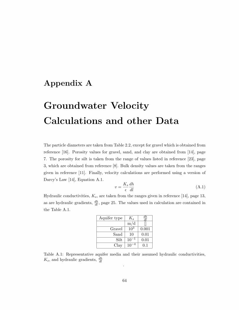
Appendix A

Groundwater Velocity

Calculations and other Data

The particle diameters are taken from Table 2.2, except for gravel which is obtained from

reference [16]. Porosity values for gravel, sand, and clay are obtained from [14], page

7. The porosity for silt is taken from the range of values listed in reference [23], page

3, which are obtained from reference [8]. Bulk density values are taken from the ranges

given in reference [11]. Finally, velocity calculations are performed using a version of

Darcy’s Law [14], Equation A.1.

v =Ks

ε

dh

dl(A.1)

Hydraulic conductivities, Ks, are taken from the ranges given in reference [14], page 13,

as are hydraulic gradients, dhdl , page 25. The values used in calculation are contained in

the Table A.1.

Aquifer type Ksdhdl

m/d []Gravel 103 0.001

Sand 10 0.01Silt 10−1 0.01

Clay 10−4 0.1

Table A.1: Representative aquifer media and their assumed hydraulic conductivities,Ks, and hydraulic gradients, dh

dl.

64

Appendix B

Groundwater Chemical Removal

For a given volume of saturated porous media, Vt, it can be shown that fp = 1 − 1R .

The properties and equations used for this are as follows.

R = 1 +ρbKd

ε(B.1)

fp =Kd[SS]

1 +Kd[SS](B.2)

ρb =MS

Vt(B.3)

Kd =Ms/MS

Mw/Vw(B.4)

ε =VwVt

(B.5)

[SS] =MS

Vw(B.6)

fp =Ms

MT(B.7)

MT = Ms +Mw (B.8)

VT = Vs + Vw (B.9)

The variables above represent the following.

ρb bulk density of porous media

65

66

ε porosity of porous media

MS mass of the solids in the given volume of porous media

Vt volume of saturated porous media

Ms mass of chemical sorbed to the solids of the porous media

Mw mass of chemical dissolved in the water saturating the porous media

Vw volume of water occupying the voids of the porous media

MT total mass of chemical

Vs volume of the solids occupying the given volume of porous media

By substituting the equations for ρb, ε, and Kd, the equation for R becomes

R = 1 +MS

Vt

Ms

MS

VwMw

VtVw

(B.10)

which can be simplified to

R = 1 +Ms

Mw(B.11)

Then, using the equation for fp and substituting the necessary values, the equation for

fp becomes

fp =MsMS

VwMw

MSVw

1 + MsMS

VwMw

MSVw

(B.12)

which simplifies to

fp =MsMw

1 + MsMw

=R− 1R

= 1− 1R

(B.13)

Using the definition of fp, that fp represents the fraction of the chemical sorbed to the

particles (in this case porous media), along with the equation for fp as a function of R

(Equation B.13), an equality that can be written is

fp =Ms

MT=R− 1R

= fp (B.14)

which gives the final equation

MT = R ∗Mw (B.15)

which shows that the total mass of a chemical in a given volume of aquifer is equivalent

to R times the mass of the chemical dissolved in the water in that given volume of

aquifer.

Appendix C

Variables and Units

Symbols

A Hamaker constant [J]

CT Total concentration of chemical, [mg/L]

d Grain size of filter media, [µm]

dp Diameter of suspended particles, [µm]

dhdl Hydraulic gradient, []

fp Fraction of the chemical associated with the particle, []

foc Fraction of organic carbon in the soil, []

g Gravity constant, [m/s2]

h Height of water body, [m]

k Boltzmann constant, [J/K]

Kd Distribution coefficient of chemical, [L/kg]

Koc Distribution coefficient of organic chemical, [L/kg]

ksed Rate of sedimentation of particles, [mg/(L*s)]

67

68

Ks Hydraulic conductivity, [m/s]

L Bed depth, distance travelled, [m]

R Retardation factor, []

[SS ] Concentration of suspended solids in water, [mg/L]

T Absolute temperature, [℃]

t1/2 Half-life of chemical or particle, [sec., min., days, years, etc.]

vs Sedimentation velocity of particles, [m/s]

v Groundwater velocity, [m/d]

Greek Letters

α Stabilization coefficient, []

ε Porosity, []

η Single collector efficiency, []

ηD, ηI , ηG Single collector efficiency for diffusion, interception, sedimentation, respectively []

µ Water viscosity, [kg/(m*s)]

ρp, ρw Density of particles and water at 10 ◦C, [kg/m3]

ρb Bulk density of aquifer, [kg/L]

an holistic approach to modelling the removal of particles

Documents