An Honest Approach to Parallel Trends ∗

Ashesh Rambachan† Jonathan Roth‡ (Job market paper)

December 18, 2019

Please click here for the latest version.

Abstract

Standard approaches for causal inference in difference-in-differences and event-studydesigns are valid only under the assumption of parallel trends. Researchers are typicallyunsure whether the parallel trends assumption holds, and therefore gauge its plausibilityby testing for pre-treatment differences in trends (“pre-trends”) between the treated anduntreated groups. This paper proposes robust inference methods that do not requirethat the parallel trends assumption holds exactly. Instead, we impose restrictions on theset of possible violations of parallel trends that formalize the logic motivating pre-trendstesting — namely, that the pre-trends are informative about what would have happenedunder the counterfactual. Under a wide class of restrictions on the possible differences intrends, the parameter of interest is set-identified and inference on the treatment effectof interest is equivalent to testing a set of moment inequalities with linear nuisanceparameters. We derive computationally tractable confidence sets that are uniformlyvalid (“honest”) so long as the difference in trends satisfies the imposed restrictions.Our proposed confidence sets are consistent, and have optimal local asymptotic powerfor many parameter configurations. We also introduce fixed length confidence intervals,which can offer finite-sample improvements for a subset of the cases we consider. Werecommend that researchers conduct sensitivity analyses to show what conclusions canbe drawn under various restrictions on the set of possible differences in trends. Weconduct a simulation study and illustrate our recommended approach with applicationsto two recently published papers.

Keywords: Difference-in-differences, event-study, parallel trends, sensitivity analysis, robust in-ference, partial identificationLink to the online appendix.∗We are grateful to Isaiah Andrews, Elie Tamer, and Larry Katz for their invaluable advice and encour-

agement. We also thank Gary Chamberlain, Raj Chetty, Peter Ganong, Ed Glaeser, Nathan Hendren, RyanHill, Ariella Kahn-Lang, Jens Ludwig, Sendhil Mullainathan, Claudia Noack, Frank Pinter, Adrienne Sabety,Pedro Sant’Anna, Jesse Shapiro, Neil Shephard, Jann Spiess, and Jim Stock for helpful comments. We grate-fully acknowledge financial support from the NSF Graduate Research Fellowship under Grant DGE1745303(Rambachan) and Grant DGE1144152 (Roth).†Harvard University, Department of Economics. Email: asheshr@g.harvard.edu‡Harvard University, Department of Economics. Email: jonathanroth@g.harvard.edu

1 Introduction

Conventional methods for causal inference in difference-in-differences and related quasi-experimentalresearch designs are valid only under the so-called “parallel trends” assumption.1 Researchers are of-ten unsure whether the parallel trends assumption is valid in applied settings, and they consequentlytry to assess its plausibility by testing for differences in trends between the treated and untreatedgroups prior to treatment (“pre-trends”). Conditional on not finding a significant pre-trend, inferenceis then typically conducted under the assumption that parallel trends holds exactly. The currentapproach to inference relying on an exact parallel trends assumption that is assessed via pre-trendstesting suffers from two broad limitations. First, inference will be misleading if in fact the paralleltrends assumption is violated but a pre-trends test fails to detect the violation (Freyaldenhoven,Hansen and Shapiro, 2019; Bilinski and Hatfield, 2018; Kahn-Lang and Lang, 2018; Roth, 2019).Second, we may still be interested in learning something about the causal effect of the treatmenteven if it is clear that there is a non-zero pre-existing trend, yet standard approaches deliver validinference in this case only under strong functional form assumptions. Both of these limitations ofthe conventional approach motivate constructing methods for inference that allow the assumptionof exact parallel trends to be relaxed.

The main contribution of this paper is to develop robust inference methods for difference-in-differences and related research designs that do not require that the parallel trends assumption holdsexactly. Instead, the researcher need only specify a set of restrictions on the possible violations ofparallel trends motivated by economic knowledge, and can conduct a sensitivity analysis to examinethe robustness of their conclusions to different assumptions about such violations. We primarilyconsider polyhedral restrictions on the difference in trends, i.e. restrictions that can be written asa system of linear inequalities. A variety of economic intuitions that commonly arise in difference-in-differences and related settings can be formalized using such restrictions. For instance, theintuition behind the common practice of testing for pre-trends is that pre-treatment differences intrends are informative about counterfactual post-treatment differences in trends – a notion that weoperationalize by restricting the degree of possible non-linearity in the difference in trends. We arealso able to incorporate intuition about simultaneous policy changes or secular trends by imposingsign or shape restrictions on the difference in trends. Under these restrictions, the treatment effectof interest is typically set-identified.

To develop uniformly valid inference methods, we exploit the novel observation that the problemof conducting inference on the treatment effect of interest in our setting is equivalent to a momentinequality problem with linear nuisance parameters. A practical challenge to testing the impliedset of moment inequalities is that the number of nuisance parameters scales linearly in the numberof post-treatment periods, and thus will often be large (above 10) in typical empirical applications.

1The parallel trends assumption states that the average outcome for the treated and untreated groupswould have moved in parallel if the treatment of interest had not occurred. This is also sometimes referredto as the “common trends” assumption (Angrist and Pischke, 2009; Lechner, 2011; Cunningham, 2018).

1

This renders many moment inequality procedures, which rely on test inversion over a grid for thefull parameter vector, computationally infeasible. Andrews, Roth and Pakes (2019a, henceforthARP) study conditional moment inequality problems with linear nuisance parameters, and proposeconfidence sets that condition on the set of sample moments that bind when using a linear programto profile out the nuisance parameters. We use this conditional inference procedure to obtaincomputationally tractable confidence sets that achieve uniform asymptotic size control. We thenexploit additional structure in our setting to derive new results on the asymptotic performance ofconditional confidence sets.2

We provide two novel results on the asymptotic properties of conditional confidence sets inour setting. First, we show that the conditional confidence sets are consistent, meaning that anyfixed point outside of the identified set is rejected with probability approaching one asymptotically.Second, we provide a condition under which the conditional confidence sets have local asymptoticpower converging to the power envelope — i.e., the upper bound on the power of any procedure thatcontrols size uniformly. Intuitively, the condition for optimality requires that the underlying trendis not aligned with a “corner” of the allowed class in a particular sense. This condition is implied by,but somewhat weaker than, linear independence constraint qualification (LICQ), which has beenused recently in the moment inequality settings of Gafarov (2019); Cho and Russell (2018); Flynn(2019); Kaido and Santos (2014).3 In contrast to many previous uses of LICQ, however, we do notrequire this condition to obtain uniform asymptotic size control. To prove the optimality result, wemake use of duality results from linear programming and the Neyman-Pearson lemma to show thatboth the optimal test and our conditional test converge to a t-test in the direction of the Lagrangemultipliers of the linear program that profiles out the nuisance parameters.

Our results on the local asymptotic power of the conditional confidence sets have two limitations.First, the condition needed for the conditional confidence sets to have optimal local asymptoticpower does not hold for all parameter values, and in particular fails when the parameter of interestis point-identified. Second, the conditional confidence sets may have low power in finite samples ifthe binding and non-binding moments are not well-separated.

We therefore introduce fixed length confidence intervals (FLCIs), which can address the lim-itations of the conditional approach in certain special cases of interest. We construct optimalFLCIs based on affine estimators for the treatment effect of interest, following Donoho (1994) andArmstrong and Kolesar (2018, 2019). We provide a novel characterization of when the optimalFLCI is consistent, meaning that any point outside of the identified set is rejected with probabilityapproaching one asymptotically: the optimal FLCI is consistent if and only if the length of theidentified set at the true population parameter equals its maximum possible length. This conditionis non-restrictive for some classes of differential trends, but is restrictive (and even provably false)

2Specifically, we make use of the fact that the moments are linear in the target parameter and that theJacobian of the moments with respect to the nuisance parameters is a known, constant matrix.

3Kaido, Molinari and Stoye (2019) show that constraint qualifications are closely related to other assump-tions used for inference in the moment inequality literature.

2

for others. When this additional condition holds, however, the optimal FLCI achieves optimallocal asymptotic power under the same conditions as the conditional confidence sets. Moreover,the optimal FLCI is near-optimal in finite sample in certain special cases of interest (Armstrongand Kolesar, 2018, 2019). In particular, the length of the optimal FLCI is close to the lower boundamong all confidence sets that control size if parallel trends holds and the class of possible underlyingdifferential trends is convex and centrosymmetric.

We next introduce a novel hybrid procedure that combines the relative strengths of the condi-tional confidence sets and FLCIs. The hybrid procedure is consistent, and has near-optimal localasymptotic power when the condition for the optimality of the conditional approach holds. More-over, we find in simulations (discussed in more detail below) that hybridization with the FLCIsimproves performance in finite sample when the moments are not well-separated. We thus recom-mend the hybrid approach for settings in which the condition for the consistency of the FLCIs isnot guaranteed.4

For ease of exposition, the main text presents our results in a finite sample normal model. Thefinite sample normal model emerges as an asymptotic approximation to a wide range of econometricsettings. In Appendix F, we show that these finite sample results translate to asymptotic results thathold uniformly over a large class of non-normal data-generating processes satisfying some high-levelregularity conditions.

To explore the performance of our methods in practice, we conduct simulations calibrated tothe 12 papers analyzed by Roth (2019), who systematically reviewed recent papers in three leadingjournals. We compute the expected excess length of each procedure, and compare this to an optimalbenchmark, which is derived using the observation that the confidence set that minimizes expectedexcess length inverts most powerful tests (Armstrong and Kolesar, 2018). We find that for manyparameter configurations, the conditional confidence sets have excess length within a few percent ofthis lower bound. However, as expected, the conditional approach can underperform in cases wherethe parameter of interest is (close to) point-identified. The FLCIs perform particularly well in thespecial cases where the conditions for their finite-sample near-optimality hold, but can have powersubstantially below the conditional test when these conditions fail; in one specification, the excesslength of the conditional confidence sets is within 2% of the optimum, whereas for the FLCIs it ismore than double the optimum. The hybrid approach performs quite well across a wide range ofspecifications — its excess length is no more than 17% larger than the other procedures across thespecifications reported in the main text, whereas each of the other two procedures is at least 50%worse than another in some specification. We thus recommend the hybrid for most cases where theconsistency of the FLCIs is not guaranteed. Lastly, all of the procedures remain computationallytractable in all specifications, including in cases with over 15 nuisance parameters.

4We also introduce a hybridization between the conditional confidence sets and tests based on leastfavorable (LF) critical values, which we recommend for cases where it is known that the FLCIs will beuninformative. Since the conditional-FLCI hybrid outperforms the conditional-LF hybrid in simulations formost parameter configurations, we focus mainly on the FLCI hybrid in the main text.

3

In practice, we recommend that applied researchers use our methods to conduct a sensitiv-ity analysis in which they report confidence sets under varying restrictions on the set of possibleviolations of parallel trends. For instance, one class of restrictions we consider requires that thedifference in trends not deviate “too much” from linearity, and is governed by a single parameterM that determines the degree of possible non-linearity. If the researcher is interested in testinga particular null hypothesis — e.g., the treatment effect in a particular period is zero — then asimple statistic to report is the “breakdown” value of M at which the null hypothesis of interestcan no longer be rejected.5 We discuss how one can benchmark the value of this parameter usingeconomic knowledge of possible confounds, as well as placebo periods or treatment groups. Theresearcher can also report how her conclusions change with the inclusion of additional sign or shaperestrictions motivated by context-specific knowledge. For instance, in cases where researchers areconcerned about secular trends correlated with treatment, researchers may specify that the under-lying difference in trends is monotone. Likewise, in cases with known simultaneous policy changes,researchers may restrict the sign of the bias. Performing such a sensitivity analysis and documentinghow the reported confidence set changes across a range of assumptions makes clear what must beassumed about the possible violations of parallel trends in order to draw specific conclusions. Ourpublicly-available R package HonestDiD provides functions for easy and fast implementation of ourrecommended methods.6

We illustrate our empirical recommendations by applying our approach to two recently-publishedpapers. First, we consider an application to Lovenheim and Willen (2019, henceforth LW), whostudy how exposure to public sector duty-to-bargain (DTB) laws as a child affects long-run labormarket outcomes. LW find no clear pre-trends for male employment, but do find substantial pre-trends for female employment, and therefore focus on their results for men. The example allowsus to illustrate how we can gauge the robustness of the results for men to different assumptions onthe possible violations of parallel trends, as well as how we can use such assumptions to constructconfidence sets for the effect on women despite the presence of a pre-trend. Second, we consider anapplication to Benzarti and Carloni (2019), who study the impact of a decrease in the value-addedtax (VAT) on the profitability of restaurants in France, and find large effects of the VAT decreaseon restaurant profitability. We show that the conclusion that restaurant profits increase in the firstyear after the VAT cut are robust to a wide range of assumptions about the underlying difference intrends, but conclusions about the longer-run effects (e.g., four years after the VAT decrease) appearto be more fragile. This illustrates a general point: when allowing for the possibility of seculardifferential trends, bias accumulates over time, and so longer-run estimates will typically be moresensitive to violations of parallel trends than short-run estimates.

5Similar “breakdown” concepts have been proposed in other partially identified settings (Horowitz andManski, 1995; Kline and Santos, 2013; Masten and Poirier, 2019).

6The latest version of the R package may be downloaded here.

4

Related Literature This paper contributes to a large and active literature on the economet-rics of difference-in-differences and related research designs by developing robust inference methodsthat allow for the possibility that parallel trends may be violated.7 Several other papers considermethods for relaxing or circumventing the assumption of exact parallel trends. Manski and Pepper(2018) consider how the set of identified parameters changes as we relax the parallel trends assump-tion, but do not consider the problem of statistical inference. Keele, Small, Hsu and Fogarty (2019)likewise develop techniques for testing the sensitivity of difference-in-differences designs to violationsof the parallel trends assumption, but they do not incorporate information from pre-trends in theirsensitivity analysis. A common approach when there are concerns about violations of the paralleltrends assumption is to adjust for the extrapolation of a linear trend from the pre-treatment pe-riod (cf. Dobkin, Finkelstein, Kluender and Notowidigdo, 2018; Goodman-Bacon, 2018a,b; Bhuller,Havnes, Leuven and Mogstad, 2013). This approach provides valid inference only under the restric-tion that the underlying trend is exactly linear. Our approach nests this restriction as a specialcase, but allows for less restrictive assumptions on the class of underlying trends; for instance,one class of restrictions we consider requires only that the linear extrapolation be approximatelycorrect. Freyaldenhoven et al. (2019) propose a method that allows for violations of the paralleltrends assumption but requires a covariate that is known to be affected by the confounds but notthe treatment of interest.8

Our robust approach to inference helps to address several concerns related to conventionalpractice in difference-in-differences and related research designs. First, a recent literature suggeststhat common tests for pre-trends may be underpowered against meaningful violations of paralleltrends, potentially leading to severe undercoverage of conventional confidential intervals, which arevalid only if parallel trends holds exactly (Freyaldenhoven et al., 2019; Bilinski and Hatfield, 2018;Kahn-Lang and Lang, 2018). For instance, Roth (2019) finds that linear violations of parallel trendsproducing bias equal to the estimated treatment effect would be detected less than half the timeby conventional pre-tests in simulations calibrated to several recent papers in leading economicsjournals. Second, statistical distortions from pre-testing for pre-trends may further underminethe performance of conventional inference procedures (Roth, 2019). Third, although there existparametric approaches to controlling for pre-existing trends, there are concerns that such methodsare sensitive to functional form assumptions (Wolfers, 2006; Lee and Solon, 2011). Our paper helpsto address these issues by providing tools for inference that do not rely on an exact parallel trends

7Previous work on inference in difference-in-differences and related designs has addressed robustness toserial correlation and clustered sampling (Arellano, 1987; Moulton, 1990; Bertrand, Duflo and Mullainathan,2004; Sun and Yan, 2019), and concerns related to having a small number of treated units (Donald and Lang,2007; Conley and Taber, 2010; Ferman and Pinto, 2018; MacKinnon and Webb, 2019), among other issues.

8In practice, one may be unsure if a covariate satisfies the exclusion restriction required by Freyaldenhovenet al. (2019). In their applications, Freyaldenhoven et al. (2019) therefore create an event-study plot thatshows estimated placebo pre-treatment effects using their method, which are analogous to pre-period coeffi-cients in a typical event-study. Since their procedure yields asymptotically normal estimates, one can applythe methods in this paper to assess the sensitivity of results using their method under various assumptionson the relationship between pre-treatment and post-treatment violations of the exclusion restriction.

5

assumption and that make clear the mapping between the restrictiveness of the assumptions on thepotential differences in trends and the strength of one’s conclusions.

Our work is also complementary to a recent literature on the causal interpretation of the iden-tified coefficients in two-way fixed effects models in settings with staggered treatment timing orheterogeneous treatment effects (Meer and West, 2016; Borusyak and Jaravel, 2016; Abraham andSun, 2018; Hull, 2018; Athey and Imbens, 2018; de Chaisemartin and D’Haultfœuille, 2018a,b;Goodman-Bacon, 2018a; Kropko and Kubinec, 2018; Callaway and Sant’Anna, 2019; Imai andKim, 2019; Słoczyński, 2018). A key finding of this literature is that regression coefficients fromconventional approaches may not produce convex weighted averages of local average treatment ef-fects even if parallel trends holds. Additionally, conventional event-study estimators may exhibitspurious pre-trends when parallel trends holds (Abraham and Sun, 2018). The literature has thusproposed a number of alternative strategies that allow for consistent estimation of sensible causalestimands under a suitable parallel trends assumption. We encourage researchers to start by choos-ing an estimation strategy that yields consistent estimates of the causal parameter of interest underthe best-case assumption of parallel trends. We then recommend using our methods to assess therobustness of conclusions to potential violations of the parallel trends assumption.9

More broadly, this paper relates to a large literature in econometrics on sensitivity analysisand misspecification robust inference. Recent work has studied misspecification in the context ofinstrumental variables models (Conley, Hansen and Rossi, 2012), generalized method of moments(Andrews, Gentzkow and Shapiro, 2017, 2019b; Armstrong and Kolesar, 2019), parametric andsemi-parametric models (Bonhomme and Weidner, 2018; Mukhin, 2018), regression discontinuitydesigns (Kolesar and Rothe, 2018; Armstrong and Kolesar, 2018), structural models (Christensenand Connault, 2019), and experimental design (Rosenbaum and Rubin, 1983; Imbens, 2003; Rosen-baum, 2005; Lee, 2009; Ding and VanderWeele, 2016), among many others. An interesting feature ofour setting is that we use restrictions to relate the degree of bias in the treatment effects estimatesfor periods after treatment to pre-trends identified in periods prior to treatment. Our approachthus shares similar structure with papers in sensitivity analysis that relate bias from selection intotreatment on unobservables to selection on observables in cross-sectional contexts (Altonji, Elderand Taber, 2005; Oster, 2019).

Finally, our work connects to the rich literature on partial identification and moment inequalityprocedures in econometrics. As in Manski and Pepper (2018), we consider relaxations of the as-sumption of exact parallel trends, under which the treatment effect of interest is partially identifiedin difference-in-differences and related settings. The use of partial identification in the analysis oftreatment effects in other observational or quasi-experimental settings dates back to at least Manski(1990), and has been used since by Balke and Pearl (1997), Heckman and Vytlacil (1999), Man-ski and Nagin (1998), Manski and Pepper (2000), Ginther (2000), González (2005), Bhattacharya,

9Our approach can be applied so long as the estimator is asymptotically normally distributed, whichcovers the vast majority of proposed procedures in difference-in-differences and related research designs.

6

Shaikh and Vytlacil (2008), Nevo and Rosen (2012), Kreider, Pepper, Gundersen and Jolliffe (2012),and Gunsilius (2019), among many others. We show that testing a null hypothesis on the treatmenteffect of interest under a relaxation of the parallel trends assumption can be cast as a moment in-equality problem, and derive novel asymptotic consistency and optimality results for confidence setsconstructed using the conditional approach of ARP. We also propose a new hybrid procedure thatcombines fixed-length confidence intervals with conditional confidence sets. This hybrid proceduremay be useful in other settings. Reviews of the wide range of applications of partial identifica-tion and moment inequality methods in economics include Manski (2003), Tamer (2010), and morerecently Ho and Rosen (2017), Canay and Shaikh (2017), and Molinari (2019).

2 Motivating example: Difference-in-differences

We begin with a stylized three-period difference-in-differences model, which allows us to highlightthe causal parameter of interest, inferential goal, and key assumptions of our approach in a simplesetting. We later introduce the general setting that will be our main focus in Section 3.

2.1 Data-generating process

We observe an outcome Yit for a sample of individuals i “ 1, . . . , N for three time periods, t “´1, 0, 1. Individuals in the treated group (Di “ 1) receive a treatment of interest between periodt “ 0 and t “ 1.10 The observed outcome can be expressed as Yit “ DiYitp1q ` p1 ´ DiqYitp0q,where Yitp1q and Yitp0q are the potential outcomes for an individual i in period t if she were or werenot assigned to the treated group. We assume that the treatment has no causal effect before it isimplemented, so that Yitp1q “ Yitp0q for t ă 1.11 We are interested in the average treatment effecton the treated (ATT) in the period after treatment, τATT “ E rYi,t“1p1q ´ Yi,t“1p0q |Di “ 1s.

In this setting, researchers commonly estimate the regression specification,

Yit “ λi ` φt `ÿ

s‰0

βs ˆ 1rt “ ss ˆDi ` εit. (1)

This specification is often referred to as a “dynamic event-study regression” or a “two-way fixedeffects model” with dynamic treatment effects (Borusyak and Jaravel, 2016; de Chaisemartin andD’Haultfœuille, 2018b). It is well-known that in this simple setting, the coefficient β1 can be writtenas the “difference-in-differences” of sample means across treated and untreated groups betweenperiod t “ 0 and t “ 1. That is, the “post-period” coefficient is

10Formally, for the purposes of this example, we think of our sample of size N “ N0 ` N1 as consistingof N1 independent draws from the treated pD “ 1q population and N0 independent draws from the controlpopulation pD “ 0q, as in Abadie and Imbens (2006).

11An important case where this could be violated is if individuals modify their behavior in anticipation ofthe reform (Malani and Reif, 2015). See Section 9 for additional discussion of anticipation.

7

β1 “ pYD“1,t“1 ´ YD“1,t“0q ´ pYD“0,t“1 ´ YD“0,t“0q,

where YD“d,t“s is the sample mean of Yit for treatment group d in period s. The “pre-period”coefficient β´1 can be expressed similarly as

β´1 “ pYD“1,t“´1 ´ YD“1,t“0q ´ pYD“0,t“´1 ´ YD“0,t“0q.

Taking expectations and re-arranging, we see that

E”

β1

ı

“ τATT ` E rYi,t“1p0q ´ Yi,t“0p0q |Di “ 1s ´ E rYi,t“1p0q ´ Yi,t“0p0q |Di “ 0slooooooooooooooooooooooooooooooooooooooooooooomooooooooooooooooooooooooooooooooooooooooooooon

Post-period differential trend :“ δ1

,

E”

β´1

ı

“ E rYi,t“´1p0q ´ Yi,t“0p0q |Di “ 1s ´ E rYi,t“´1p0q ´ Yi,t“0p0q |Di “ 0slooooooooooooooooooooooooooooooooooooooooooooooomooooooooooooooooooooooooooooooooooooooooooooooon

Pre-period differential trend :“ δ´1

.

Thus, the post-period regression coefficient β1 is biased for the treatment effect τATT if δ1 ‰ 0. Thebias δ1 is the differential trend in outcomes for the two groups between period 0 and period 1 thatwould have occurred if the treatment counterfactually did not take place. Likewise, δ´1 is the pre-period differential trend between groups from period 0 to period ´1. The parallel trends assumptionimposes that the expectation of Yitp0q moves in parallel for the two groups, δ´1 “ δ1 “ 0, in whichcase β1 is unbiased for the treatment effect of interest.

2.2 Inferential goal

Applied to this illustrative three period difference-in-differences example, this paper considers theproblem of conducting inference on τATT while relaxing the assumption that δ1 is exactly zero. Ofcourse, if we allow δ1 to be completely unrestricted, then the data will be uninformative about thevalue of τATT . However, the motivating logic behind the common practice of pre-trends testingis that the pre-period difference in trends δ´1 is informative about the counterfactual post-perioddifference in trends δ1. We thus may be willing to place restrictions on the possible values of δ1

given δ´1.We formalize this intuition by assuming that δ “ pδ´1, δ1q

1P ∆, where ∆ is some class of possible

differential trends that is specified by the researcher. The usual parallel trends assumption is thusthe special case where ∆ “ t0u. Given a set ∆, we then construct confidence sets that are uniformlyvalid over a wide class of distributions with δ P ∆. That is, for P a class of distributions P suchthat δ P ∆ under P, we construct confidence sets Cn satisfying

lim infnÑ8

infPPP

PP pτ P Cnq ě 1´ α. (2)

8

A confidence set Cn that satisfies this criterion is sometimes referred to as “uniform” or “honest”(Andrews, Cheng and Guggenberger, Forthcoming; Li, 1989; Armstrong and Kolesar, 2018).

In practice, the class of allowed differential trends ∆ will often be parameterized by M , whichindexes the extent to which the counterfactual post-period difference in trends can differ froman extrapolation of the pre-period difference in trends. We recommend that researchers reportconfidence sets under a variety of values of M to give the reader a sense of how much regularityneeds to be imposed ex ante to obtain informative inference. We now discuss a few specificationsfor ∆ that may be reasonable in empirical applications.

2.3 Possible choices of ∆

The class of possible violations of parallel trends ∆ must be specified by the researcher, and thechoice of ∆ will depend on the economic context. Here, we highlight several choices of ∆ thatmay be reasonable in applications. These examples formalize intuitive arguments that are madein the literature regarding possible violations of parallel trends. We discuss possible restrictionsin the stylized three-period model presented above, and also discuss how these restrictions can begeneralized to cases with multiple periods, as will be common in applications.

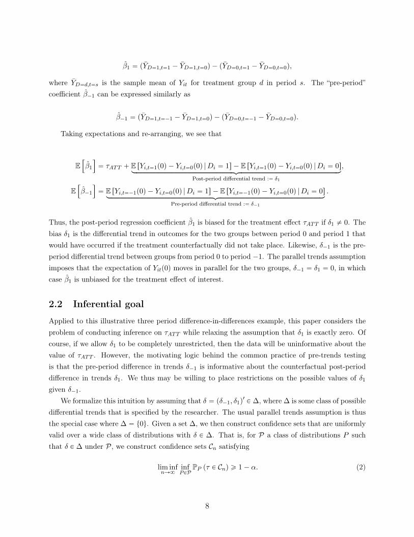
Bounds on changes in slope. In practice, researchers concerned about possible violationsof the parallel trends assumption often include treatment-group specific linear trends.12 In themotivating three period model, such an approach will recover the causal parameter τATT under theassumption that the differential trend is exactly linear, δ1 “ ´δ´1, as shown in Figure 1. Thereare concerns, however, that this linear extrapolation of the pre-period trend to the post-periodmay not hold exactly (Wolfers, 2006; Lee and Solon, 2011). A natural relaxation of the lineartrend model is to require only that the linear extrapolation be approximately correct, meaning thatδ1 P r´δ´1´M,´δ´1`M s, whereM governs the maximum possible error of the linear extrapolation(i.e. the change in slope of the differential trend). This corresponds with setting ∆ equal to

∆SDpMq :“ tpδ´1, δ1q1 : δ1 P ´δ´1 ˘Mu.

This restriction can easily be extended to settings with additional periods by bounding theextent to which the slope of the differential trend can change between consecutive periods. Forinstance, in Section 3 we consider a more general model where the researcher estimates

¯T pre-event

12That is, instead of estimating specification (1), researchers estimate

Yit “ λi ` φt ` βtrend ˆDi ˆ t`ÿ

są0

βs ˆ 1rt “ ss ˆDi ` εit,

which Dobkin et al. (2018) refer to as a “parametric event-study.” An analogous approach is to estimate alinear trend using only observations prior to treatment, and then subtract out the estimated linear trendfrom the observations after treatment (Bhuller et al., 2013; Goodman-Bacon, 2018a,b).

9

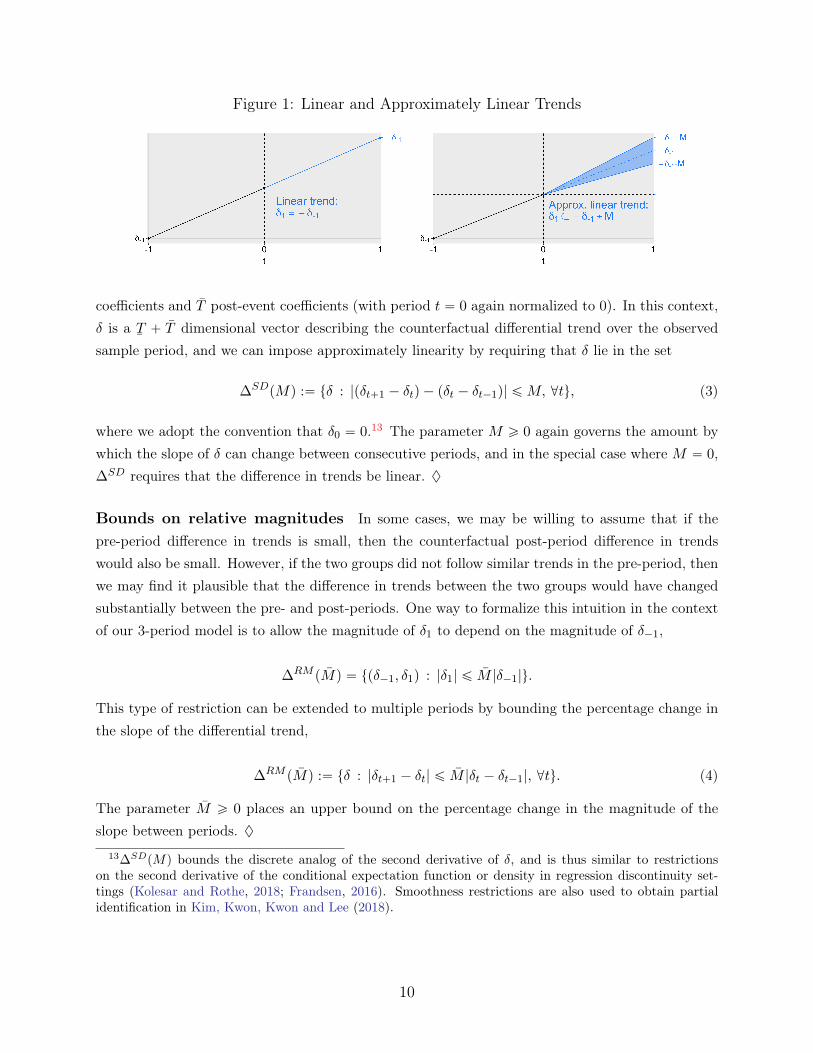
Figure 1: Linear and Approximately Linear Trends

coefficients and T post-event coefficients (with period t “ 0 again normalized to 0). In this context,δ is a

¯T ` T dimensional vector describing the counterfactual differential trend over the observed

sample period, and we can impose approximately linearity by requiring that δ lie in the set

∆SDpMq :“ tδ : |pδt`1 ´ δtq ´ pδt ´ δt´1q| ďM, @tu, (3)

where we adopt the convention that δ0 “ 0.13 The parameter M ě 0 again governs the amount bywhich the slope of δ can change between consecutive periods, and in the special case where M “ 0,∆SD requires that the difference in trends be linear. ♦

Bounds on relative magnitudes In some cases, we may be willing to assume that if thepre-period difference in trends is small, then the counterfactual post-period difference in trendswould also be small. However, if the two groups did not follow similar trends in the pre-period, thenwe may find it plausible that the difference in trends between the two groups would have changedsubstantially between the pre- and post-periods. One way to formalize this intuition in the contextof our 3-period model is to allow the magnitude of δ1 to depend on the magnitude of δ´1,

∆RM pMq “ tpδ´1, δ1q : |δ1| ď M |δ´1|u.

This type of restriction can be extended to multiple periods by bounding the percentage change inthe slope of the differential trend,

∆RM pMq :“ tδ : |δt`1 ´ δt| ď M |δt ´ δt´1|, @tu. (4)

The parameter M ě 0 places an upper bound on the percentage change in the magnitude of theslope between periods. ♦

13∆SDpMq bounds the discrete analog of the second derivative of δ, and is thus similar to restrictionson the second derivative of the conditional expectation function or density in regression discontinuity set-tings (Kolesar and Rothe, 2018; Frandsen, 2016). Smoothness restrictions are also used to obtain partialidentification in Kim, Kwon, Kwon and Lee (2018).

10

Figure 2: Example choices for ∆

δ1

δ´1

∆SD

δ1

δ´1

∆RM

δ1

δ´1

∆SDPB

δ1

δ´1

∆RMI

Note: This figure shows diagrams of potential restrictions ∆ on the set of possible violations of paralleltrends. ∆SD requires approximate linearity by restricting the change in slope of the differential trend. ∆RM

bounds the magnitude of the post-period bias relative to the magnitude of the pre-trend. ∆SDPB addsthe restriction that the post-period bias be positive to ∆SD. Likewise, ∆RMI adds the restriction that thedifferential trend be increasing over time to ∆RM .

Sign and monotonicity restrictions Context-specific knowledge may sometimes imply signor shape restrictions on the differential trend. For instance, suppose we know of a simultaneous,confounding policy change that we expect would have a positive effect on the outcome of interest.In this case, we might restrict that the bias in the post-treatment period be positive,

δ P ∆PB :“ tδ : δt ě 0 @t ě 0u.

Likewise, it may be reasonable to impose monotonicity in cases where we are concerned aboutsecular trends that we expect would have continued following the date of treatment.14 For instance,we could impose that the differential trend be increasing,

14The discussion of possible violations of parallel trends in applied work often implicitly assumes mono-tonicity. For example, Lovenheim and Willen (2019) argue that violations of parallel trends cannot explaintheir results because “pre-[treatment] trends are either zero or in the wrong direction (i.e., opposite to the di-rection of the treatment effect).” Greenstone and Hanna (2014) estimate upward-sloping pre-existing trendsand argue that “if the pre-trends had continued” their estimates would be upward biased. The so-calledAshenfelter (1978)’s dip in job training programs is a well-known exception wherein we expect violations ofparallel trends to be non-monotonic.

11

δ P ∆I :“ tδ : δt ě δt´1 @tu.

These sign and monotonicity restrictions can also be combined with the bounds on changes in slopeor relative magnitudes imposed above. For example, we will define ∆SDPBpMq :“ ∆SDpMqX∆PB

and ∆RMIpMq :“ ∆RM pMq X∆I . ♦

Figure 2 gives a geometric depiction of the sets ∆SD,∆RM ,∆SDPB, and ∆RMI in the simple casein which there is one pre-period and one post-period coefficient.

3 General Set-up

We now introduce the assumptions, target parameter, and inferential goal considered throughout theremainder of the paper. We consider a finite-sample normal model, which arises as an approximationto the motivating model discussed in Section 2 and to a variety of other econometric settings ofinterest. In Appendix F, we show that our results derived in the context of the finite-sample normalmodel hold uniformly over a large class of non-normal data-generating processes.

3.1 Finite sample normal model

We consider the model,

βn „ N pβ, Σnq , (5)

where βn P R¯T`T , and Σn “

1nΣ˚ for Σ˚ a known, positive-definite p

¯T ` T q ˆ p

¯T ` T q matrix. We

partition the event-study coefficients βn into vectors corresponding with the pre-treatment and post-treatment periods, βn “ pβ1n,pre, β1n,postq1, where βn,pre P R¯

T and βn,post P RT . We adopt analogousnotation to partition other vectors that are the same length as βn into pre and post components.

This finite sample normal model (5) can be viewed as an asymptotic approximation to a widerange of econometric settings. In particular, under mild regularity conditions, a variety of estimationstrategies will yield asymptotically normal event-study estimates,

?n´

βn ´ β¯

dÝÑ N p0, Σ˚q.15

This convergence in distribution suggests the finite-sample approximation βnd« N pβ, Σnq , where

d« denotes approximate equality in distribution and Σn “

1nΣ˚. In the main text of the paper, we

derive results assuming this equality in distribution holds exactly in finite samples, and in Appendix

15Examples of data-generating processes that yield asymptotically normal event-study estimates includethe two-way fixed effects model (1), the GMM procedure proposed by Freyaldenhoven et al. (2019), instru-mental variables event-studies (Hudson, Hull and Liebersohn, 2017), the estimation strategies of Abrahamand Sun (2018) and Callaway and Sant’Anna (2019) to address issues with non-convex weights on cohort-specific effects in staggered treatment designs, as well as a range of procedures that flexibly control fordifferences in covariates between treated and untreated groups (e.g., Heckman, Ichimura, Smith and Todd,1998; Abadie, 2005; Sant’Anna and Zhao, 2019).

12

F, we translate our results into uniform asymptotic statements that hold over a large class of non-normal data-generating processes.

We assume that the mean vector β satisfies the following decomposition.

Assumption 1. The parameter vector β can be decomposed as

β “

˜

τpre

τpost

¸

loooomoooon

:“ τ

`

˜

δpre

δpost

¸

loooomoooon

:“ δ

, (6)

with τpre ” 0.

The first term, τ , represents the time path of dynamic causal effects of interest. We assume thatthe treatment has no causal effect prior to its implementation, so τpre “ 0. The second term,δ, represents the difference in trends between the treated and untreated groups that would haveoccurred absent treatment.16 In this general setting, the parallel trends assumption corresponds toimposing that δ “ 0. Therefore, under parallel trends, β “ τ .

3.2 Target parameter and identification

The parameter of interest is a scalar, linear combination of the post-treatment causal effects, θ :“

l1τpost for some known T -vector l. For example, the parameter θ is the t-th period causal effect τtwhen the vector l equals the t-th standard basis vector. Similarly, θ is the average causal effectacross all of the post-treatment periods when l “

`

1T, ..., 1

T

˘1. Under the usual exact parallel trendsassumption (δ “ 0), θ is point-identified.

We relax the exact parallel trends assumption by assuming only that δ lies in some set ofpossible violations of parallel trends ∆, which is specified by the researcher. The usual paralleltrends assumption is thus a special case with ∆ “ t0u. Under the assumption that δ P ∆ ‰ t0u, theparameter θ will typically only be set-identified (rather than point-identified). For a given value ofβ, the set of values θ consistent with β under the assumption that δ P ∆ is

Sp∆, βq :“

#

θ : Dδ P ∆, τpost P RT s.t. l1τpost “ θ, β “ δ `

˜

0

τpost

¸+

, (7)

which we refer to as the identified set.We note that the identified set has a simple characterization when ∆ is a convex set. In

particular, it is clear from (7) that if ∆ is convex, then so too is Sp∆, βq, and thus the identified

16In settings with staggered treatment timing and treatment effect heterogeneity, the vector τpost that isidentified by a two-way fixed effects specification may represent some weighted sum of cohort-specific effects.Researchers should take care to specify their estimator in such a way that τpost has a meaningful, causalinterpretation. See, e.g., recent work by Abraham and Sun (2018), among others.

13

set is an interval in R. Furthermore, re-arranging terms in the definition given in (7), the identifiedset can be equivalently written as

Sp∆, βq “ tθ : Dδ P ∆ s.t. δpre “ βpre, θ “ l1βpost ´ l1δpostu. (8)

It is then immediate from (8) that the lower bound of the interval S is

θlb :“ l1βpost ´

ˆ

maxδl1δpost, s.t. δ P ∆, δpre “ βpre

˙

loooooooooooooooooooooooomoooooooooooooooooooooooon

“:bmaxpβpre;∆q

. (9)

Likewise, the upper bound is given by

θub :“ l1βpost ´

ˆ

minδl1δpost, s.t. δ P ∆, δpre “ βpre

˙

looooooooooooooooooooooomooooooooooooooooooooooon

“:bminpβpre;∆q

. (10)

3.3 Inferential goal

Our goal is then to construct confidence sets that are valid for all parameter values θ in the identifiedset. That is, we wish to construct sets Cn satisfying

infδP∆,τ

infθPSp∆,δ`τq

Ppδ,τ,Σnq pθ P Cnq ě 1´ α, (11)

which is the finite-sample analog of the uniform asymptotic coverage criterion (2). Although inthe main text we focus on this finite-sample coverage criterion, in Appendix F we show how ourfinite-sample coverage results translate to uniform asymptotic coverage results over a wide classof non-normal data-generating processes. We note that (11) requires proper coverage of the trueparameter of interest θ “ l1τpost, rather than coverage of the full identified set (Imbens and Manski(2004)). Note also that in (11), we subscript the probability operator by pδ, τ,Σnq to make explicitthat the distribution of βn (and hence Cn) depends on these parameters. We adopt this notationthroughout the paper.

4 Conditional Confidence Sets

In this section, we describe our main procedure for constructing robust confidence sets. We focus onthe case where the set of possible violations ∆ takes the polyhedral form, ∆ “ tδ : Aδ ď du, whichcovers many leading examples. We first show that when the set ∆ takes this form, the problemof conducting robust inference in difference-in-differences and event-study designs is equivalent toa moment inequality problem with linear nuisance parameters. The dimension of the nuisanceparameters scales linearly with the number of post-treatment periods, and thus will frequently be

14

large (above 10) in practical applications. We next show that the conditioning approach of ARP,which exploits the linear structure of the problem, can be used to obtain confidence sets that satisfythe uniform coverage restriction (11) and remain computationally tractable in practice. In Section5, we then derive novel results on the power of this procedure in our context.

4.1 Polyhedral forms for ∆

As mentioned, we focus on classes ∆ that take a polyhedral form, meaning it can be expressed asa series of linear restrictions on δ.

Assumption 2 (Polyhedral shape restriction). The class ∆ takes the form

∆ “ tδ : Aδ ď du, (12)

for some matrix A and vector d, where the matrix A has no all-zero rows.

While this assumption is not without loss of generality, all but one of the leading examples providedin Section 2.3 can be written in this form. Intuitively, the set ∆ is a polyhedron if it is a convexset with flat sides. It is thus immediate from Figure 2 that with two dimensions, ∆SD,∆SDPB,

and ∆RMI can all be written as polyhedra, and the geometric intuition from the two-period caseextends easily to higher dimensions.17 We also can see from Figure 2 that ∆RM is not convex andthus not a polyhedron, although it can be expressed as the union of polyhedra. One can thus forma confidence set for ∆RM by taking the union of the confidence sets for each of the polyhedra thatcompose it.

4.2 Representation as a moment inequality problem with linear nui-

sance parameters

Consider the problem of testing the null hypothesis, H0 : θ “ θ, δ P ∆ when ∆ “ tδ : Aδ ď du. Inthis section, we will show that testing H0 is equivalent to testing a system of moment inequalitieswith linear nuisance parameters.

Our model implies Epδ,τ,Σnq”

βn ´ τı

“ δ, and hence δ P ∆ if and only if Epδ,τ,Σnq”

Aβn ´Aτı

ď

d. Define Yn “ Aβn ´ d and let Mpost “ r0, Is1 be the matrix such that τ “ Mpostτpost. It is then

immediate that the null hypothesis H0 is equivalent to the composite null

H0 : Dτpost P RT s.t. l1τpost “ θ and Epδ,τ,Σnq rYn ´AMpostτposts ď 0. (13)

17For example, recall that |x| ďM is equivalent to x ďM and ´x ďM . In the case with one pre-period

and one post-period, we can thus write ∆SDpMq “ tδ : ASDδ ď dSDu for ASD “

ˆ

´1 11 ´1

˙

and

dSD “

ˆ

MM

˙

. This generalizes naturally when there are multiple pre-periods and multiple post-periods.

15

Here, τpost P RT is a vector of nuisance parameters that must satisfy the linear constraint l1τpost “ θ

under H 10.By applying a change of basis, we can further re-write H0 as an equivalent composite null

hypothesis with an unconstrained nuisance parameter. In particular, we can re-write the expression

AMpostτpost as A

˜

θ

τ

¸

, where A is the matrix that results from applying a suitable change of basis

to the columns of AMpost, and τ P RT´1.18 We then see that H0 is equivalent to

H0 : Dτ P RT´1 s.t. E”

Ynpθq ´ Xτı

ď 0, (14)

where Y pθq “ Yn ´ Ap¨,1qθ and X “ Ap¨,´1q. Note that under the finite-sample normal model (5),Ynpθq is normally distributed with covariance matrix Σn “ AΣnA

1. We therefore have shown thattesting the null hypothesis H0 : θ “ θ is equivalent to testing a set of moment inequalities withlinear nuisance parameters.

4.3 Constructing conditional confidence sets

An important practical consideration for testing hypotheses of the form (14) is that the dimension ofthe nuisance parameter τ P RT´1 may be large in practice. For instance, in Section 10 we considera recent paper in which T “ 23. Moreover, 5 of the 12 recent event-study papers reviewed in Roth(2019) have T ą 10. This renders many moment inequality methods, particularly those which relyon test inversion over a grid for the full parameter vector, practically infeasible in this context. Wenow show how the conditional approach of ARP, which directly exploits the linear structure of thehypothesis (14), can be applied to obtain computationally tractable and powerful tests even whenthe number of post-periods T is large.19

To describe the conditional testing approach, suppose we wish to test (14) for some fixed θ. Theconditional testing approach considers tests based on the test statistic

η :“ minη,τ

η s.t. Ynpθq ´ Xτ ď σn ¨ η, (15)

where σn “b

diagpΣnq. This linear program selects the value of the nuisance parameters τ P RT´1

18Specifically, let Γ be a square matrix with the vector l1 in the first row and remaining rows chosen so

that Γ has full rank. Define A :“ AMpostΓ´1. Then AMpostτ “ AΓτpost “ A

¨

˝

θΓp´1,¨qτpostlooooomooooon

:“τ

˛

‚.

19Other moment inequality methods have been proposed for subvector inference, but typically do notexploit the linear structure of our setting — see, e.g, Chen, Christensen and Tamer (2018); Bugni, Canayand Shi (2017); Kaido et al. (2019); Chernozhukov, Newey and Santos (2015); Romano and Shaikh (2008).Gafarov (2019), Cho and Russell (2018), and Flynn (2019) also provide methods for subvector inferencewith linear moment inequalities, but in contrast to our approach require a linear independence constraintqualification (LICQ) assumption for size control.

16

that produces the most slack in the maximum moment, measured in standard deviation units.Standard duality results from linear programming (e.g. Schrijver (1986), Section 7.4) imply that ifthe value η obtained from the so-called primal linear program (15) is finite, then it is equal to theoptimal value of the dual program,

η “ maxγ

γ1Ynpθq s.t. γ1X “ 0, γ1σn “ 1, γ ě 0. (16)

If a vector γ˚ is optimal in the dual problem above, then it is a vector of Lagrange multipliers forthe primal problem. We will denote by Vn the set of optimal vertices of the dual program.20

To derive critical values for our test, we analyze the distribution of η conditional on the eventthat a vertex γ˚ is optimal in the dual problem. Lemma 9 of ARP shows that conditional on theevent γ˚ P Vn and a sufficient statistic Sn for the nuisance parameters, the test statistic η follows atruncated normal distribution. In particular,

η | tγ˚ P Vn, Sn “ su „ ξ | ξ P rvlo, vups, (17)

where ξ „ N´

γ1˚µ, γ1˚Σnγ˚

¯

, µ “ E”

Ynpθqı

, Sn “ pI ´ Σnγ˚γ1˚Σnγ˚

γ1˚qYnpθq, and vlo, vup are known

functions of Σn, s, γ˚.21 One can show that all quantiles of the conditional distribution of η in theprevious display are increasing in γ1˚µ,22 and the null hypothesis (14) implies that γ1˚µ ď 0.

We therefore select the critical value for the conditional test to be the 1 ´ α quantile of thetruncated normal distribution ξ|ξ P rvlo, vups under the worst-case assumption that γ1˚µ “ 0. Tospecify this formally, denote by Fξ | ξPrvlo,vupsp¨;σ2q the CDF of ξ „ N

`

0, σ2˘

truncated to rvlo, vups.Let ψCα pYnpθq, Σnq denote an indicator for whether the conditional test rejects at the 1 ´ α level.We define the conditional test such that

ψCα pYnpθq, Σnq “ 1 ðñ Fξ | ξPrvlo,vupspη; γ1˚Σnγ˚q ą 1´ α. (18)

It follows immediately from Proposition 6 in ARP that the conditional test controls size,

supδP∆,τ

supθPSp∆,δ`τq

Epδ,τ,Σnq”

ψCα pYnpθq, Σnq

ı

ď α. (19)

A confidence set satisfying the uniform coverage criterion (11) can then be constructed by test

20In general, there may not be a unique solution to the dual program. However, Lemma 11 of ARP showsthat conditional on any one vertex of the dual program’s feasible set being optimal, every other vertex isoptimal with either probability 0 or 1. It thus suffices to condition on the event that a vector γ˚ P V .

21The cutoffs vlo and vup are the maximum and minimum of the set tx : x “ maxγPFn γ1ps` Σnγ˚

γ1˚Σnγ˚xqu

when γ1˚Σnγ˚ ‰ 0, where Fn is the feasible set of the dual program (16). When γ1˚Σnγ˚ “ 0, we definevlo “ ´8 and vup “ 8, so the conditional test rejects if and only if η ą 0.

22This follows from the fact that the truncated normal distribution ξ|ξ P rvlo, vups has the monotonelikelihood ratio property in it is mean (see, e.g. Lemma A.1 in Lee, Sun, Sun and Taylor (2016)).

17

inversion for the scalar parameter θ. The conditional confidence set is given by

CCα,n :“ tθ : ψCα pYnpθq, Σnq “ 0u. (20)

Remark 1. For each value of θ, the test statistic η can be computed by solving the linear program(15). To form the confidence set CCα,n, one only needs to perform test inversion over a grid of valuesfor the scalar parameter θ, and thus the problem remains highly tractable even when T is large.Moreover, the commonly-used dual simplex algorithm for linear programming returns a vertex tothe dual solution (16), so an optimal dual vertex γ˚ can be obtained from standard packages withoutfurther calculation. We provide R code for easy implementation of this procedure.

Remark 2. To gain intuition for the conditional test, consider the simple setting in which we haveone post-period pT “ 1q and are interested in the treatment effect in the first period, θ “ τ1. In thiscase, there are no nuisance parameters, and the form of the conditional test simplifies substantially.The test statistic η is the maximum of the standardized moments, η “ maxj Yn,j{σn,j , whereσn,j is the standard deviation of Yn,j . The conditional test rejects in this case if and only ifΦpηq´Φpvloq

1´Φpvloqą 1´ α. Moreover, if the moments Yn are uncorrelated with each other, then vlo is the

maximum of the non-binding standardized moments, vlo “ maxj‰j Yn,j{σn,j , where j denotes thelocation of the maximum standardized moment. �

5 Asymptotic Power of Conditional Confidence Sets

We now analyze the properties of the conditional confidence sets. For ease of exposition, we considerlimits as nÑ8 in the finite-sample normal model defined in Section 3.23 In Appendix F, we showthat these results hold uniformly over a wide class of non-normal data-generating processes.

We present two main results on the asymptotic power of the conditional confidence sets. Wefirst show that the conditional test is pointwise consistent, meaning that any point outside of theidentified set is rejected with probability going to one as nÑ8. We next provide a condition underwhich the power of the conditional test converges to the power envelope in a n´1{2-neighborhoodof the identified set.

Both our consistency and local asymptotic power results are novel, and exploit additional struc-ture in our problem not present in the somewhat more general setting considered in ARP. ARPconsider testing null hypotheses of the form H0 : Dτ s.t. E rY pθq ´Xτ |Xs ď 0, almost surely. Oursetting, in which we are interested in testing the hypothesis (14), is thus a special case of the testingproblem considered by ARP in which i) the variable X takes the degenerate distribution X “ X,and ii) Y pθq “ Y pθq is linear in θ. Both of these features are important for the results obtained inthis section. For instance, if i) fails and X is continuously distributed, then the tests proposed by

23The results in this section as nÑ 8 for βn „ N`

β, 1nΣ˚

˘

are similar in spirit to the “small-σ” asymp-totics in e.g., Kadane (1971); Moreira and Ridder (2019).

18

ARP will generally not be consistent, as they do not allow for the number of moments to grow withn. Likewise, our local asymptotic power results exploit the geometric structure imposed by featuresi) and ii).

5.1 Consistency

We first show that the conditional test is consistent, meaning that any fixed point outside of theidentified set is rejected with probability approaching one as the sample size nÑ8.

Proposition 5.1. The conditional test is consistent. That is, for any δA P ∆, τA P RT , andθout R Sp∆, δA ` τAq,

limnÑ8

PpδA,τA,Σnq`

θout R CCα,n˘

“ 1.

We present this result for fixed values of pδA, τAq for ease of exposition. Proposition F.3 in AppendixF shows that the conditional test is uniformly consistent for points at a fixed distance from theidentified set over a wide class of data-generating processes.

5.2 Optimal Local Asymptotic Power

We next consider the local asymptotic power of the conditional test. We provide a condition underwhich the power of the conditional test converges to the power envelope in a n´

12 -neighborhood of

the identified set. Intuitively, this condition guarantees that the binding and non-binding momentsare sufficiently well-separated at points close to the boundary of the identified set.

Assumption 3. Let ∆ “ tδ : Aδ ď du and fix δA P ∆. Consider the optimization:

bmaxpδA,preq “ maxδl1δpost s.t. Aδ ď d, δpre “ δA,pre,

and assume it has a finite solution. For δ˚ a maximizer to the above problem, let Bpδ˚q index theset of binding inequality constraints, so that ApBpδ˚q,¨qδ˚ “ dBpδ˚q and Ap´Bpδ˚q,¨qδ

˚ ´ d´Bpδ˚q “

´ε´Bpδ˚q ă 0. Assume that there exists a maximizer δ˚ to the problem above such that the rank ofApBpδ˚q,postq is equal to |Bpδ˚q|. Analogously, assume that there is a finite solution to the analogousproblem that replaces max with min, and that there is a minimizer δ˚˚ such that ApBpδ˚˚q,postq hasrank |Bpδ˚˚q|.

Assumption 3 considers the problem of finding the differential trend δ P ∆ that is consistent with thepre-trend identified from the data (δA,pre) and causes l1βpost to be maximally biased for θ :“ l1τpost.It requires that the “right” number of moments bind when we do this optimization.

19

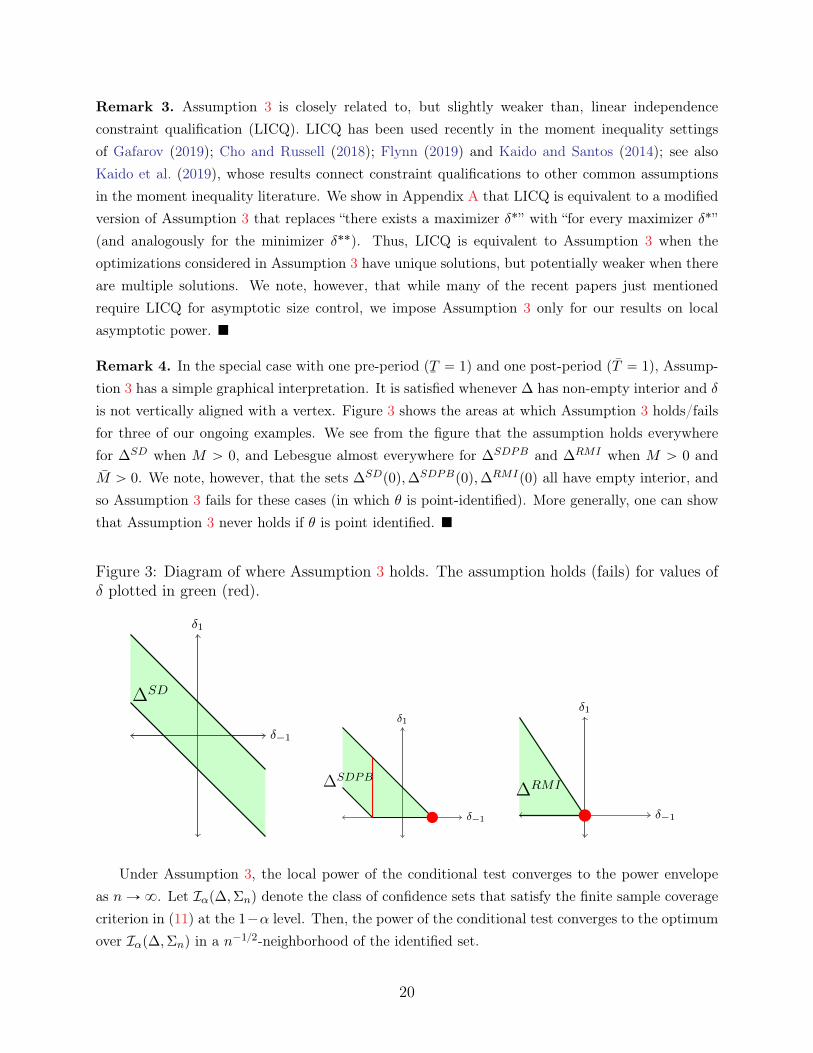
Remark 3. Assumption 3 is closely related to, but slightly weaker than, linear independenceconstraint qualification (LICQ). LICQ has been used recently in the moment inequality settingsof Gafarov (2019); Cho and Russell (2018); Flynn (2019) and Kaido and Santos (2014); see alsoKaido et al. (2019), whose results connect constraint qualifications to other common assumptionsin the moment inequality literature. We show in Appendix A that LICQ is equivalent to a modifiedversion of Assumption 3 that replaces “there exists a maximizer δ˚” with “for every maximizer δ˚”(and analogously for the minimizer δ˚˚). Thus, LICQ is equivalent to Assumption 3 when theoptimizations considered in Assumption 3 have unique solutions, but potentially weaker when thereare multiple solutions. We note, however, that while many of the recent papers just mentionedrequire LICQ for asymptotic size control, we impose Assumption 3 only for our results on localasymptotic power. �

Remark 4. In the special case with one pre-period p¯T “ 1q and one post-period pT “ 1q, Assump-

tion 3 has a simple graphical interpretation. It is satisfied whenever ∆ has non-empty interior and δis not vertically aligned with a vertex. Figure 3 shows the areas at which Assumption 3 holds/failsfor three of our ongoing examples. We see from the figure that the assumption holds everywherefor ∆SD when M ą 0, and Lebesgue almost everywhere for ∆SDPB and ∆RMI when M ą 0 andM ą 0. We note, however, that the sets ∆SDp0q,∆SDPBp0q,∆RMIp0q all have empty interior, andso Assumption 3 fails for these cases (in which θ is point-identified). More generally, one can showthat Assumption 3 never holds if θ is point identified. �

Figure 3: Diagram of where Assumption 3 holds. The assumption holds (fails) for values ofδ plotted in green (red).

δ1

δ´1

∆SD

δ1

δ´1

∆SDPB

δ1

δ´1

∆RMI

Under Assumption 3, the local power of the conditional test converges to the power envelopeas nÑ8. Let Iαp∆,Σnq denote the class of confidence sets that satisfy the finite sample coveragecriterion in (11) at the 1´α level. Then, the power of the conditional test converges to the optimumover Iαp∆,Σnq in a n´1{2-neighborhood of the identified set.

20

Proposition 5.2. Fix δA P ∆, τA, and suppose Σ˚ is positive definite. Let θubA “ supθ Sp∆, δA`τAqbe the upper bound of the identified set. Suppose Assumption 3 holds. Then, for any x ą 0,

limnÑ8

PpδA,τA,Σnqˆ

pθubA `1?nxq R CCα,n

˙

“ limnÑ8

supCα,nPIαp∆,Σnq

PpδA,τA,Σnqˆ

pθubA `1?nxq R Cα,n

˙

“ Φpc˚x´ z1´αq,

for a positive constant c˚.24 The analogous result holds replacing θubA `1?nx with θlbA ´

1?nx, for θlbA

the lower bound of the identified set (although the constant c˚ may differ).

Proposition F.4 in Appendix F shows that this result holds uniformly over a large class of distri-butions that satisfy a uniform version of Assumption 3, meaning that the non-binding moments inthe problem bmax are uniformly bounded away from binding.

5.2.1 Intuition for local asymptotic optimality

We now sketch the intuition for why the local asymptotic power of the conditional test convergesto the power envelope. For simplicity, we focus on the simple case with one pre-period and onepost-period. Recall from Remark 4 that in this case, Assumption 3 implies that a single momentdetermines the upper bound of the identified set. The argument that the local asymptotic power ofthe conditional test converges to the power envelope then proceeds in two steps. First, we show thatthe optimal test converges to a t-test of the moment that determines the boundary of the identifiedset. Next, we show that the power of the conditional test converges to the power of this same t-test.

First, focus on the form of the optimal test. Consider the problem of testing the compositenull hypothesis H0 : τ1 “ τ1, δ P ∆ against the point alternative HA : pδ, τ1q “ pδA, τAq. Since bydefinition, β “ δ`Mpostτ1, this is equivalent to testing H0 : β P B0pτ1q “ tβ : β “ δ`Mpostτ1, δ P

∆u against HA : β “ δA `MpostτA “: βA. It can be shown that B0 is convex, and so the Neyman-Pearson lemma implies that the most powerful test between H0 and HA is a t-test that rejects forlarge values of pβA´ βq1Σ´1

n βn, where β is the closest point in B0 to βA in the Mahalanobis distanceusing Σn. Moreover, if β is in the interior of a side of B0 (i.e. not at a vertex), then this t-test ismerely a one-sided t-test of the sample moment corresponding with that edge. Figure 4 depicts thistesting problem for when ∆ “ ∆RMIpMq. As shown in the figure, Assumption 3 implies that βAfalls in the interior of an edge of B0pτ

ubq. By continuity, for n sufficiently large, the closest point inB0pτ

ub` x{?nq will also fall in the interior of that edge. Hence, the most powerful test against HA

will be a one-sided t-test of the moment that determines the upper bound of the identified set.

24In particular, letting B “ Bpδ˚˚q as defined in Assumption 3, c˚ “ ´γ1BApB,1q{σB , where σB “b

γ1BApB,¨qΣ˚A1

pB,¨qγB and γB is a non-zero vector such that γ1BApB,´1q “ 0, γB ě 0. The vector γB isunique up to scale.

21

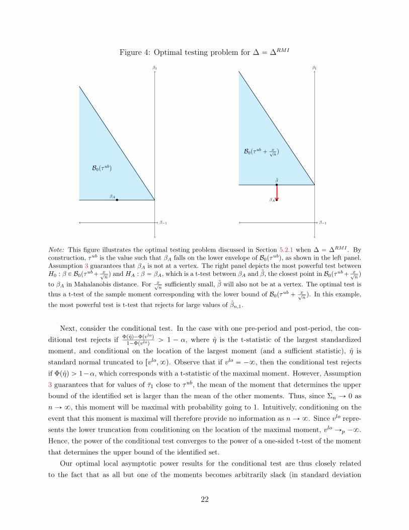
Figure 4: Optimal testing problem for ∆ “ ∆RMI

β1

β´1

βA

B0pτubq

β1

β´1

βA

β

B0pτub ` x?

nq

Note: This figure illustrates the optimal testing problem discussed in Section 5.2.1 when ∆ “ ∆RMI . Byconstruction, τub is the value such that βA falls on the lower envelope of B0pτ

ubq, as shown in the left panel.Assumption 3 guarantees that βA is not at a vertex. The right panel depicts the most powerful test betweenH0 : β P B0pτ

ub` x?nq and HA : β “ βA, which is a t-test between βA and β, the closest point in B0pτ

ub` x?nq

to βA in Mahalanobis distance. For x?nsufficiently small, β will also not be at a vertex. The optimal test is

thus a t-test of the sample moment corresponding with the lower bound of B0pτub ` x?

nq. In this example,

the most powerful test is t-test that rejects for large values of βn,1.

Next, consider the conditional test. In the case with one pre-period and post-period, the con-ditional test rejects if Φpηq´Φpvloq

1´Φpvloqą 1 ´ α, where η is the t-statistic of the largest standardized

moment, and conditional on the location of the largest moment (and a sufficient statistic), η isstandard normal truncated to rvlo,8q. Observe that if vlo “ ´8, then the conditional test rejectsif Φpηq ą 1´α, which corresponds with a t-statistic of the maximal moment. However, Assumption3 guarantees that for values of τ1 close to τub, the mean of the moment that determines the upperbound of the identified set is larger than the mean of the other moments. Thus, since Σn Ñ 0 asn Ñ 8, this moment will be maximal with probability going to 1. Intuitively, conditioning on theevent that this moment is maximal will therefore provide no information as nÑ8. Since vlo repre-sents the lower truncation from conditioning on the location of the maximal moment, vlo Ñp ´8.Hence, the power of the conditional test converges to the power of a one-sided t-test of the momentthat determines the upper bound of the identified set.

Our optimal local asymptotic power results for the conditional test are thus closely relatedto the fact that as all but one of the moments becomes arbitrarily slack (in standard deviation

22

units), the conditional test converges in probability to a one-sided t-test of the binding moment (seeProposition 3 in ARP). To our knowledge, this feature is not shared by any other existing momentinequality procedure that controls size in the finite sample Gaussian model. Specifically, althoughrelatively insensitive to the inclusion of slack moments, the procedures of Romano, Shaikh and Wolf(2014) and Andrews and Barwick (2012) are still affected by the inclusion of slack moments via thefirst-stage critical value and size-adjustment factor, respectively. The method of Cox and Shi (2019)is strongly insensitive to the inclusion of slack moments, but does not converge to a one-sided t-testas the other moments become slack.

5.3 Power in Finite Samples

While the conditional confidence sets have desirable asymptotic properties as the sample size nÑ8,our results provide no guarantees on their performance in finite samples. Moreover, we anticipatethat the conditional test may have low power in finite samples for cases in which Assumption 3 failsor is “close to failing,” meaning that the binding and non-binding moments are not well-separatedrelative to the sampling variation. An important case where this will occur is when the parameterof interest θ is point-identified.

To develop intuition for why this may occur, we return to the simple case considered in Remark2 in which there is only one post-period, the parameter of interest is the treatment effect in the firstperiod, and the elements of Y are uncorrelated. Recall that in this example, the conditional testrejects if and only if Φpηq´Φpvloq

1´Φpvloqą 1 ´ α, where the test statistic η is the maximum standardized

sample moment and vlo is the value of the second-largest standardized sample moment. Note thatif the difference in means between the two largest moments is small (relative to their variance),then we will have that η « vlo with high probability, in which case the conditional test may notreject even if the test statistic η is large. This suggests that the conditional approach may have lowpower in finite-samples if there are multiple moments that are close to binding at the edge of theidentified set. Recall that when Assumption 3 fails, there are multiple moments that are exactlybinding at the identified set bound. We thus should expect the conditional approach to have poorpower in finite samples in a neighborhood of points where Assumption 3 fails, where the size of theneighborhood depends on the sampling variation. This is a generic challenge for the conditionaltesting approach, and we show that it can lead to poor power in some cases in our simulation studyin Section 8.

Owing to this limitation, we next turn our attention to fixed length confidence intervals (FL-CIs), which can offer finite-sample improvements in certain special cases of interest, but requirestronger assumptions to obtain the asymptotic guarantees of the conditional approach. Lookingahead, we will then show how the conditional confidence sets can be hybridized with FLCIs orleast-favorable tests to mitigate poor performance when the moments are not well-separated whileretaining desirable asymptotic properties in a wider range of cases.

23

6 Finite-sample Improvements Using FLCIs

We now consider fixed length confidence intervals (FLCIs) based on affine estimators. Although theFLCIs require additional assumptions to obtain similar asymptotic performance to the conditionalconfidence sets, they provide finite-sample guarantees for certain special cases of interest.

6.1 Constructing FLCIs

Following Donoho (1994) and Armstrong and Kolesar (2018, 2019), we consider fixed length confi-dence intervals based on an affine estimator for θ,

Cα,npa, v, χq “´

a` v1βn

¯

˘ χ, (21)

where a and χ are scalars and v P R¯T`T . We wish to minimize the confidence interval half-length

χ subject to the constraint that Cα,npa, v, χq satisfies the coverage requirement (11). To do so, notethat a`v1βn „ N pa` v1β, v1Σnvq, and hence |a`v1βn´θ| „ |N pb, v1Σnvq |, where b “ a`v1β´θ

is the bias of the affine estimator a ` v1β for θ. Observe further that θ P Cnpa, v, χq if and only if|a` v1βn ´ θ| ď χ. For fixed values a and v, the smallest value of χ that satisfies (11) is thereforethe 1 ´ α quantile of the |N

`

b, v1Σnv˘

| distribution, where b is the worst-case bias of the affineestimator,

bpa, vq :“ supδP∆,τpostPRT

|a` v1pδ `Mpostτpostq ´ l1τpost|. (22)

Let cvαptq denote the 1´ α quantile of the folded normal distribution |N pt, 1q |.25 Then, for fixeda and v, the smallest value of χ that satisfies the coverage requirement (11) is

χnpa, v;αq “ σv,n ¨ cvαpbpa, vq{σv,nq, (23)

where σv,n :“?v1Σnv.

We can therefore construct the minimum length FLCI by choosing the values of a and v tominimize (23). Intuitively, this minimization optimally trades off bias and variance, since thehalf-length χnpa, v;αq is increasing in both the worst-case bias b and the variance σ2

v,n (assumingα P p0, 0.5sq. When ∆ is convex, this minimization can be solved as a nested optimization problem,where both the inner and outer minimizations are convex (Low, 1995; Armstrong and Kolesar, 2018,2019), and is thus simple to compute. We denote by CFLCIα,n the 1´ α level FLCI with the shortestlength,

CFLCIα,n “

´

an ` v1nβn

¯

˘ χn,

25If t “ 8, we define cvα “ 8.

24

where χn :“ infa,v χnpa, v;αq and an, vn are the optimal values in the minimization.

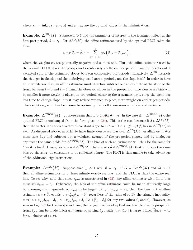
Example: ∆SDpMq Suppose T ě 1 and the parameter of interest is the treatment effect in thefirst post-period, θ “ τ1. For ∆SDpMq, the affine estimator used by the optimal FLCI takes theform

a` v1βn “ βn,1 ´0ÿ

s“´¯T`1

ws

´

βn,s ´ βn,s´1

¯

, (24)

where the weights ws are potentially negative and sum to one. Thus, the affine estimator used bythe optimal FLCI takes the post-period event-study coefficient for period 1 and subtracts out aweighted sum of the estimated slopes between consecutive pre-periods. Intuitively, ∆SD restrictsthe changes in the slope of the underlying trend across periods, not the slope itself. In order to havefinite worst-case bias, an affine estimator must therefore subtract out an estimate of the slope of thetrend between t “ 0 and t “ 1 using the observed slopes in the pre-period. The worst-case bias willbe smaller if more weight is placed on pre-periods closer to the treatment date, since the trend hasless time to change slope, but it may reduce variance to place more weight on earlier pre-periods.The weights ws will then be chosen to optimally trade off these sources of bias and variance.

Example: ∆SDPBpMq Suppose again that T ě 1 with θ “ τ1. In the case ∆ “ ∆SDPBpMq, theoptimal FLCI is unchanged from the form given in (24). This is the case because if δ P ∆SDpMq,then the vector that adds a vector of constant slope to δ, δ “ δ` c ¨ p´

¯T, ..., T q1, lies in ∆SDpMq as

well. As discussed above, in order to have finite worst-case bias over ∆SDpMq, an affine estimatormust take βn,1 and subtract out a weighted average of the pre-period slopes, and by analogousargument the same holds for ∆SDPBpMq. The bias of such an estimator will thus be the same forδ as it is for δ. Hence, for any δ P ∆SDpMq, there exists δ P ∆SDPBpMq that produces the samebias by choosing the constant c to be sufficiently large. The FLCI is thus unable to take advantageof the additional sign restrictions.

Example: ∆RMIpMq Suppose that T ě 1 with θ “ τ1. If ∆ “ ∆RMIpMq and M ą 0,then all affine estimators for τ1 have infinite worst-case bias, and the FLCI is thus the entire realline. To see why, note that since τpost is unrestricted in (22), any affine estimator with finite biasmust set vpost “ e1. Otherwise, the bias of the affine estimator could be made arbitrarily largeby choosing the magnitude of τpost to be large. But, if vpost “ e1, then the bias of the affineestimator a` v1βn equals |a` v1preδpre ` δ1| regardless of the value of τ . By the triangle inequality,maxt|a ` v1preδpre ` δ1|, |a ` v1preδpre ` δ1|u ě

12 |δ1 ´ δ1| for any two values δ1 and δ1. However, as

seen in Figure 2 for the two-period case, the range of values of δ1 that are feasible given a pre-periodtrend δpre can be made arbitrarily large by setting δpre such that |δ´1| is large. Hence bpa, vq “ 8for all choices of pa, vq.

25

6.2 Consistency and Local Asymptotic Power

We now consider the performance of the optimal FLCIs as n Ñ 8, as we did in Section 5 for theconditional confidence sets. As made clear by the example for ∆RMI above, in which the FLCIalways has infinite length, the FLCIs will not necessarily be consistent (nor optimal) without addi-tional restrictions. We show that the FLCIs obtain similar asymptotic properties to the conditionalconfidence set if and only if the length of the identified set at δ equals its maximal length over allpossible violations in the class ∆.

First, recall from the discussion in Section 3.2 that when ∆ is convex, the identified set is aninterval. Further, observe from (9) and (10) that the length of the identified set is θub ´ θlb “

bmaxpβpre; ∆q ´ bminpβpre; ∆q, which depends only on ∆ and βpre. We will therefore denote byLIDp∆;βpreq the length of the identified set. As we will show, the optimal FLCI shares the desirableasymptotic behavior of the ARP confidence sets when δpre is such that the length of the identifiedset is maximal and finite.

Assumption 4 (Identified set maximal length and finite). Suppose δpre is such that LIDp∆, δpreq “supδpreP∆pre

LIDp∆, δpreq ă 8.

Remark 5. In our two-period examples, the length of the identified set corresponds with theheight of ∆, and so Assumption 4 holds if and only if ∆ achieves its maximal height at δ´1. Figure5 shows where this is the case for three of our ongoing examples. As can be seen, the assumptionholds everywhere for ∆SD, for values of δ where the sign restrictions do not bind for ∆SDPB, andnowhere for ∆RMI . The restrictiveness of Assumption 4 thus depends greatly on ∆. �

Figure 5: Diagram of where Assumptions 4 and 5 hold. The values of δ are colored red(neither holds), light green (Assumption 4 only), and dark green (both hold).

δ1

δ´1

∆SDδ1

δ´1

∆SDPB

δ1

δ´1

∆RMI

Our next result shows CFLCIα,n is consistent if and only if Assumption 4 holds, provided that theidentified set is not the equal to the real line (in which case any procedure that controls size isconsistent).

26

Proposition 6.1. Suppose that ∆ is convex and α P p0, .5s. Fix δA P ∆ and τA P RT , and supposeSp∆, δA ` τAq ‰ R. Then Assumption 4 holds if and only if CFLCIα,n is consistent, meaning for allθout R Sθp∆, δA ` τAq,

limnÑ8

PpδA,τA,Σnq`

θout P CFLCIα,n

˘

“ 0.

Moreover, if Assumption 4 holds in addition to the conditions in Proposition 5.2, then the FLCIhas local asymptotic power approaching the power envelope.

Proposition 6.2. Fix δA P ∆, τA P RT and suppose Σ˚ is positive definite. Let θubA “ supθ Sp∆, δA`τAq be the upper bound of the identified set. Suppose that Assumption 3 holds and δA,pre satisfiesAssumption 4. Then, for any x ą 0 and α P p0, 0.5s,

limnÑ8

PpδA,τA,Σnqˆ

pθubA `1?nxq R CFLCIα,n

˙

“ limnÑ8

supCα,nPIαp∆,Σnq

PpδA,τA,Σnqˆ

pθubA `1?nxq R Cα,n

˙

.

The analogous result holds replacing θubA `1?nx with θlbA´

1?nx, for θlbA the lower bound of the identified

set.

Thus, we see that CFLCIα,n behaves similarly to CCα,n as n Ñ 8 when Assumption 4 holds, but it isotherwise inconsistent in the strong sense that points outside of the identified set are rejected withnon-vanishing probability asymptotically.

6.3 Finite-sample near-optimality

While the FLCIs require stronger conditions to produce the same behavior asymptotically as theconditional confidence sets, an advantage of the FLCIs is that Armstrong and Kolesar (2018, 2019)establish finite-sample near-optimality results for particular cases of interest. The following result,which is an immediate consequence of results in Armstrong and Kolesar (2018, 2019), bounds theratio of the expected length of the shortest possible confidence interval that controls size relative tothe length of the optimal FLCI.

Assumption 5. Assume that i) ∆ is convex and centrosymmetric (i.e. δ P ∆ implies ´δ P ∆),and ii) δA P ∆ is such that pδ ´ δAq P ∆ for all δ P ∆.

Proposition 6.3. Suppose δA and ∆ satisfy Assumption 5. Then, for any τA P RT , Σ˚ positivedefinite, and n ą 0,

infCα,nPIαp∆,Σnq EpδA,τA,Σnq rλpCα,nqs2χn

ě pz1´αp1´ αq ´ zαΦpzαq ` φpz1´αq ´ φpzαqq{z1´α{2,

where λp¨q denotes the length (Lebesgue measure) of a set and zα “ z1´α ´ z1´α{2.

27

Part i) of Assumption 5 is satisfied for ∆SD but not for our other ongoing examples. For example,∆SDPB and ∆RMI are convex but not centrosymmetric, and ∆RM is neither convex nor centrosym-metric. Part ii) of Assumption 5 is always satisfied when parallel trends holds pδA “ 0q. It also holdswhenever δA is a linear trend for the case of ∆SDpMq. We show in Lemma E.29 in the Appendixthat the conditions of Proposition 6.3 imply that Assumption 4 holds. Thus, the FLCIs obtainfinite sample near-optimality in a subset of the cases where they are consistent.

We note that Assumption 5 does not necessarily rule out point identification. For instance, itis satisfied when ∆ “ ∆SDp0q, which restricts that the differential trend be linear. Recall thatAssumption 3 fails when θ is point-identified, and so the conditional approach may have low powerin such cases. We thus anticipate that FLCIs will outperform the conditional confidence sets inpoint-identified cases where Assumption 5 holds.

Finally, for α “ 0.05, the lower bound in Proposition 6.3 evaluates to 0.72, so the expectedlength of the shortest confidence possible interval that satisfies the coverage requirement (11) is atmost 28% shorter than the length of the optimal FLCI.

6.4 Comparison to conditional confidence sets

The results above and in the previous section highlight tradeoffs between the conditional confidencesets and FLCIs. The conditional confidence sets are consistent and have optimal local asymptoticpower under weaker conditions than the FLCIs, but may have low power in finite samples if themoments are not well-separated. By contrast, when the stronger conditions for consistency aresatisfied, the FLCIs additionally have desirable finite-sample guarantees when ∆ is convex andcentrosymmetric. The balance of these tradeoffs depends on the choice of ∆, as can be seen fromthe examples discussed in Section 6.2. At one extreme, there are special cases — such as ∆SD —in which Assumption 4 is non-restrictive and the conditions for finite sample-near optimality hold.The FLCIs are preferable in these special cases, as they have similar asymptotic properties to theconditional approach but also offer finite-sample guarantees. At the other extreme, there are cases— such as ∆RMI — where the FLCIs are never consistent and thus are undesirable. Matters aresomewhat less clear for intermediate cases between these two extremes. For ∆SDPB, the FLCIsare consistent for some values of δ but not for others. One can also construct sets ∆ for which theconditions for consistency and finite-sample near-optimality of the FLCIs hold for some values ofδ P ∆ but for other values of δ the FLCIs are inconsistent.26

To address these intermediate cases, we now turn our attention to hybridized conditional con-fidence sets, which mitigate the power issues of the conditional confidence sets when the momentsare not well-separated while largely retaining their desirable asymptotic properties.

26For instance, consider the two-period case where ∆ “ ∆SDpMq X tδ : |δ1| ďMu. Then Proposition 6.3holds for δ “ 0, but Assumption 4 fails for any δ P ∆ with δ´1 ‰ 0.

28

7 Conditional-FLCI Hybrid Confidence Sets

We showed in Section 5 that the conditional approach has generally desirable asymptotic properties,but may perform poorly in finite samples if the moments are not well-separated. In Section 6, weshowed that FLCIs are an attractive alternative with finite sample guarantees for certain specialcases of interest, but may be inconsistent outside of these special cases. It is therefore natural toask whether it is possible to mitigate the poor performance of the conditional approach when themoments are not well-separated while retaining its desirable asymptotic properties.

To address this goal, we now propose a novel confidence set that hybridizes the conditionaltest with the optimal FLCI. This conditional-FLCI hybrid confidence set achieves similar desirableasymptotic properties as the conditional confidence set. Moreover, we find in simulations (discussedin the following section) that it leads to substantial improvements in the power of the conditionaltest in a variety of cases where the moments are not well-separated.

In the Appendix, we also consider a hybridization between conditional confidence sets andleast-favorable critical values, which may be useful in cases, such as ∆RMI , where we know thatthe FLCI will be uninformative. Because we only find moderate improvements of this conditionalleast-favorable confidence set relative to the conditional confidence set in simulations, we defer thedetails to Appendix C.

7.1 Constructing Conditional-FLCI Hybrid Confidence Sets

The conditional-FLCI hybrid confidence set is constructed by first testing whether a candidateparameter value lies within the optimal level-p1´ κq FLCI, and then applying a conditional test toall parameter values that lie within the optimal FLCI. In the second stage, we use a modified versionof the conditional test that i) adjusts size to account for the first-stage test, and ii) conditions onthe event that the first-stage test fails to reject.27

Formally, suppose that 0 ă κ ă α. Consider the level p1 ´ κq optimal FLCI, CFLCIκ,n “ an `

v1nβn ˘ χn. Lemma B.2 shows that the distribution of the test statistic η defined in (15) follows atruncated normal distribution conditional on the parameter value θ falling within the level p1´ κqoptimal FLCI. More concretely,

η |!

γ˚ P Vn, Sn “ s, θ P CFLCIκ,n

)

„ ξ | ξ P rvloC-FLCI , vupC-FLCIs, (25)

where ξ „ N´

γ1˚µ, γ1˚Σnγ˚

¯

, vloC-FLCI , vupC-FLCI are defined in Lemma B.2, γ˚ is a vector of Lagrange

multipliers for the primal problem (16), and Sn is the sufficient statistic for the nuisance parametersas defined in Section 4. With this result, the construction of the second-stage of the conditional-FLCI hybrid test is analogous to the construction of the conditional test, except it uses the modified

27In simulations, we find that adjusting the conditioning event in the second stage yields better performancein terms of excess length than simply Bonferroni-adjusting the second-stage conditional test.

29

size α “ α´κ1´κ , which accounts for the first-stage test. Formally, the conditional-FLCI hybrid test

ψC-FLCI is defined as

ψC-FLCIκ,α pβn, θ, Σnq “ 1 ðñ

θ R CFLCIκ,n , OR Fξ | ξPrvloC-FLCI ,vupC-FLCI s

pη; γ1˚Σnγ˚q ą 1´ α,

where, as in Section 4, Fξ | ξPrvloC-FLCI ,vupC-FLCI s

p¨; γ1˚Σnγ˚q denotes the CDF of a ξ „ N´

0, γ1˚Σnγ˚

¯

truncated to rvloC-FLCI , vupC-FLCIs.

Since the FLCI controls size, the first stage test rejects with probability at most κ under thenull that θ “ θ. Likewise, by the same argument as for the conditional test, the second-stage testrejects with probability at most α “ α´κ

1´κ conditional on θ P CFLCIκ,n . Together these results implythat the conditional-FLCI hybrid test controls size,

supδP∆,τ

supθPSp∆,δ`τq

Epδ,τ,Σnq”

ψC-FLCIκ,α pβn, θ, Σnq

ı

ď α. (26)

Therefore, we can construct a conditional-FLCI hybrid confidence set for the parameter θ thatsatisfies (11) by inverting the conditional-FLCI test,

CC-FLCIκ,α,n “ tθ : ψC-FLCI

κ,α pβn, θ, Σnq “ 0u. (27)

7.2 Asymptotic power of the conditional-FLCI hybrid confidence

sets

We now show that the conditional-FLCI hybrid confidence sets have asymptotic properties similarto those of the conditional test. First, the conditional-FLCI hybrid is consistent.

Proposition 7.1. The conditional-FLCI hybrid test is consistent. That is, for any δA P ∆, τA P RT ,θout R Sp∆, δA ` τAq, α P p0, .5s, and κ P p0, αq,

limnÑ8

PpδA,τA,Σnq`

θout R CC-FLCIκ,α,n

˘

“ 1.

Second, when Assumption 3 holds, the local asymptotic power of the conditional-FLCI hybrid is atleast as good as the power of the optimal level p1´ αq confidence set. Thus, when the first-stage κis small, the power of the conditional-FLCI hybrid is near the power envelope.

Proposition 7.2. Fix δA P ∆, τA, and Σ˚ positive definite. Suppose Assumption 3 holds. Supposeα P p0, .5s, κ P p0, αq, and let α “ α´κ

1´κ . Then,

lim infnÑ8

PpδA,τA,Σnqˆ

pθubA `1?nxq R CC-FLCI

κ,α,n

˙

ě limnÑ8

supCα,nPIαp∆,Σnq

PpδA,τA,Σnqˆ

pθubA `1?nxq R Cα,n

˙

.

30

The analogous result holds replacing θubA `1?nx with θlbA´

1?nx, for θlbA the lower bound of the identified

set (although the constant c˚ may differ).

8 Simulation study

In this section, we present a series of simulations calibrated to 12 recent papers illustrating therelative performance of the confidence sets discussed above and comparing them to an optimalbenchmark.

8.1 Simulation Design

Our simulations are calibrated using the estimated covariance matrix from the 12 papers surveyedin Roth (2019). Roth (2019) systematically reviewed the set of papers containing an event-studyplot published in the American Economic Review, AEJ: Applied Economics and AEJ: EconomicPolicy between 2014 and mid-2018, and analyzed 12 (out of a total of 70) for which replication datawas available and other criteria (such as reporting standard errors) were met.28 For any given paperin the survey, we will denote by Σ the estimated variance-covariance matrix from the event-studyin the paper, calculated using the clustering scheme specified by the authors. We then simulateevent-study coefficients βs from a normal model under the assumption of parallel trends pδ “ 0q

and zero treatment effects pτpost “ 0q, βs „ N´

0, Σ¯

. The choice of zero treatment effect is only anormalization, since all of the methods considered are equivariant to shifts in τpost. In simulation s,we then construct confidence intervals using the pair pβs, Σq for each of our proposed procedures.In all of our simulations, we use nominal 95% confidence intervals.29

We conduct simulations in this finite-sample normal model with known covariance for bothpractical and substantive reasons. We do this because we expect the normal approximation to be areasonable approximation to finite-sample behavior in this setting, and because there are tractablebenchmarks for the optimal performance of confidence sets in this context. To examine the quality ofthe normal approximation, in Appendix H.2 we report results from a set of simulations calibratedto the empirical distribution of the first paper in our survey, in which the covariance matrix isestimated from the data. There, we find that the finite-sample performance of the procedures westudy is indeed well-approximated by that in the normal model.

For a given choice of ∆, we compute the identified set Sp∆, 0q and calculate the expectedexcess length for each of the proposed confidence sets. The excess length of a confidence set Cpβqis the length of the part of the confidence set that falls outside of the identified set, defined asELpC; βq “ λpCpβqzSp∆, 0qq. We benchmark the expected excess length of our proposed proceduresrelative to the optimal bound over confidence sets that satisfy the uniform coverage requirement (11).

28See Section 4.1 of Roth (2019) for a detailed discussion of the sample selection criteria for this survey ofpublished event studies.

29Following Romano et al. (2014) and ARP, we use κ “ α{10 for our hybrid procedures.

31

A formula for this optimal bound is provided in Appendix D, and follows from results in Armstrongand Kolesar (2018), which use the observation that the confidence set that minimizes expected(excess) length inverts most powerful (Neyman-Pearson) tests for each candidate parameter value.For each paper, we conduct 1000 simulations and compute the optimal bound and the averageexcess length for the conditional confidence set, FLCI, and conditional-FLCI hybrid confidence set.We then define the excess length efficiency for each procedure to be the ratio of the optimal boundto the simulated expected excess length. In the main text, we report the efficiency ratios for themedian paper in the survey. Figures in Appendix H show the maximum and minimum over thepapers in the survey.

We consider three choices of ∆ to highlight the performance of the confidence sets across a rangeof conditions. Table 1 summarizes which of our theoretical results hold for each of the simulationdesigns. We first consider sets of the form ∆ “ ∆SDpMq. In this simulation design, the conditionshold for all three procedures to be consistent, and they all have (near-)optimal local asymptoticpower provided M ą 0. The conditions also hold for the FLCIs to have near-optimal expectedlength in finite sample. Next, we consider sets of the form ∆ “ ∆SDPBpMq. Under this simulationdesign, the conditional (hybrid) confidence sets are again consistent, and are asymptotically (near-)optimal when M ą 0. However, the conditions needed for the FLCI to be consistent do not holdwhen M ą 0. Finally, we consider sets of the form ∆ “ ∆SDIpMq, which combines ∆SD with therestriction that δ be increasing. In this final specification, only the conditions for the consistencyof the conditional and hybrid confidence sets hold. None of the criteria needed for asymptotic orfinite-sample optimality are satisfied, and the FLCIs are inconsistent when M ą 0.

∆SD ∆SDPB ∆SDI

Conditional / HybridConsistent X X XAsymptotically (near-)optimal X X ˆ

FLCIConsistent X ˆ ˆ

Asymptotically (near-)optimal X ˆ ˆ

Finite-sample near-optimal X ˆ ˆ

Table 1: Summary of expected properties for each simulation design

Finally, for each choice of ∆, the units of the parameter M are standardized to equal thestandard error of the first post-period event study coefficient pσ1q. We show results for a variety ofchoices of M{σ1. All of the procedures considered and the optimal bounds are invariant up to scalein the sense that the confidence set using pM, 1

nΣ˚q is 1n times the confidence set using pnM,Σ˚q.

Thus, our simulation results on excess length asM{σ1 grows large are isomorphic to our asymptoticresults presented earlier in which nÑ8 for Σn “

1nΣ˚ and M ą 0 fixed. They also, however, have

a finite-sample interpretation, illustrating how our results change as we allow the set of underlyingtrends to be more non-linear, holding Σ˚ constant. In the main text, the parameter of interest in

32

all simulations is the causal effect in the first post-period (θ “ τ1).In Appendix H, we present several extensions to the main simulation exercise discussed here.

First, we repeat the simulation study, setting the parameter of interest to be the average causaleffect across all post-periods (θ “ τpost), with qualitatively similar results. Second, we present resultsfor the conditional-least favorable hybrid discussed briefly in Section 7 and detailed in AppendixC. Finally, we present simulation results for ∆ “ ∆RMIpMq. This choice of ∆ illustrates theperformance of our proposed confidence sets in a case in which the FLCI is always infinite length,but the conditional and hybrid approaches remain consistent.

8.2 Simulation Results

Results for ∆SDpMq: The top panel of Figure 6 plots the efficiency ratio for each of ourprocedures as a function of M{σ1 when ∆ “ ∆SD. As expected, all of the procedures perform wellasM{σ1 grows large, with the efficiency ratios approaching 1. This illustrates our asymptotic (near-)optimality results for all the procedures considered in this simulation design. The FLCIs also performquite well for smaller values of M{σ1, including the point-identified case where M “ 0, illustratingthe finite-sample near-optimality results for the FLCIs when Assumption 5 holds. Although theconditional confidence sets have efficiency approaching the optimal bound for M{σ1 large, theirefficiency whenM{σ1 “ 0 is only about 50%. This reflects the fact that whenM “ 0, the parameteris point-identified and so Assumption 3 fails, leading to low power for the conditional test. We seethat the conditional-FLCI hybrid substantially improves efficiency for small values of M{σ1, whilestill retaining near-optimal performance as M{σ1 grows large.

Results for ∆SDPBpMq: The middle panel of Figure 6 plots the efficiency ratio for each of ourprocedures as a function ofM{σ1 when ∆ “ ∆SDPB. Again, the efficiency ratios for the conditionaland hybridized confidence sets are (near-)optimal asM{σ1 grows large, highlighting our asymptotic(near-)optimality results for these procedures in this simulation design. However, the efficiencyratios for the FLCIs steadily decrease as M{σ1 increases, which reflects the fact that the FLCIsare not consistent in this simulation design when M ą 0. We again see that the conditional-FLCIhybrid improves efficiency when M{σ1 is small, while retaining near-optimal performance as M{σ1

grows large.

Results for ∆SDI The bottom panel of Figure 6 plots the efficiency ratio for each of our proce-dures as a function of M{σ1 when ∆ “ ∆SDI . As discussed above and summarized in Table 1, theconditions for asymptotic (near-)optimality do not hold for any of our procedures in this simulationdesign. Nonetheless, we see that the conditional and hybrid procedures still perform quite well forlarge values of M{σ1, with efficiency approaching about 90%. We find this evidence encouraging asit shows that they may perform well asymptotically in cases where Assumption 3 fails. We againsee that the efficiency of the FLCIs degrades as M{σ1 grows, reflecting the fact that the FLCIs are

33

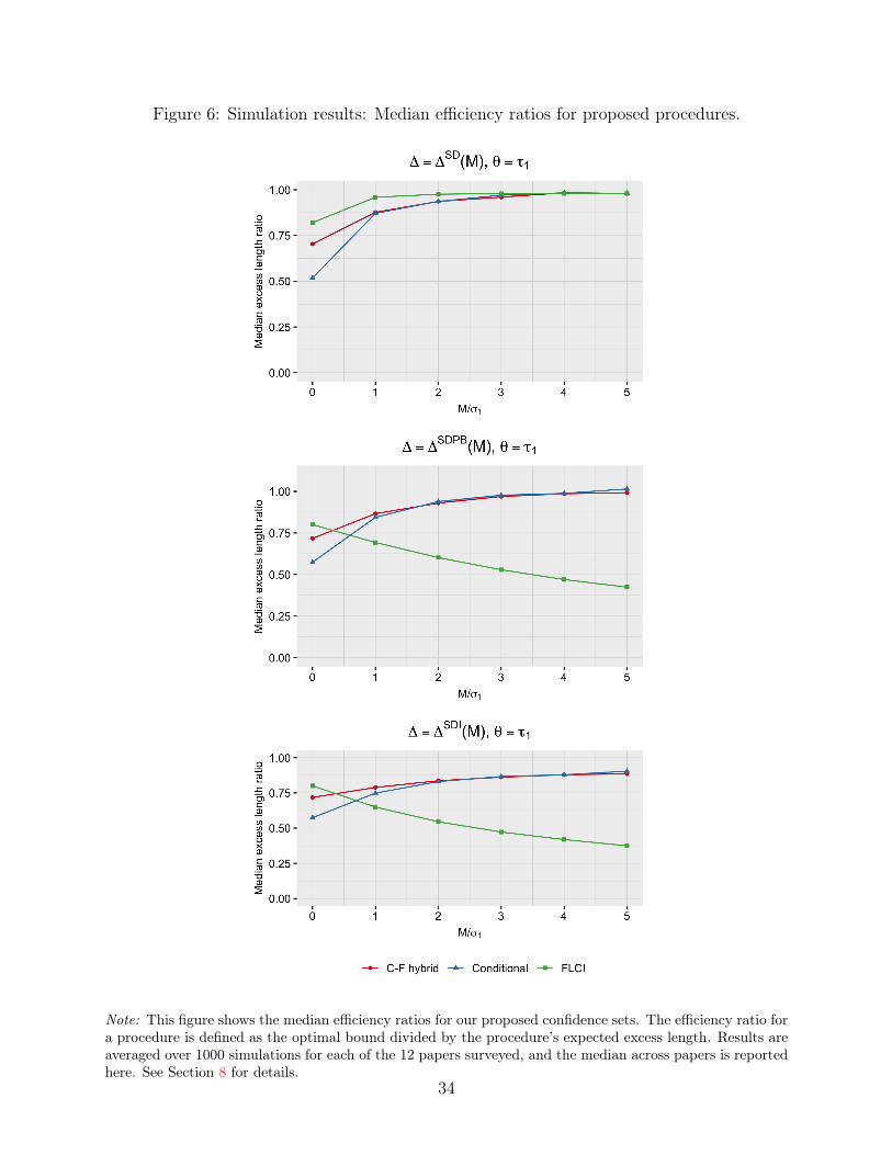
Figure 6: Simulation results: Median efficiency ratios for proposed procedures.

Note: This figure shows the median efficiency ratios for our proposed confidence sets. The efficiency ratio fora procedure is defined as the optimal bound divided by the procedure’s expected excess length. Results areaveraged over 1000 simulations for each of the 12 papers surveyed, and the median across papers is reportedhere. See Section 8 for details.

34

inconsistent under this simulation design when M ą 0. Finally, we note that as in the previoussimulations, the conditional-FLCI hybrid improves efficiency when M{σ1 is small, while retainingsimilar performance to the conditional approach as M{σ1 grows large.

8.3 Key takeaways from the simulation study

Summarizing our results from the simulation study, we find that the conditional confidence setsperform well across a range of applications but can have low power when the moments are notwell-separated. In contrast, the FLCIs perform well in terms of excess length when the neededconditions for consistency and finite-sample optimality are satisfied (e.g. ∆SDpMq) but performquite poorly elsewhere (e.g. ∆SDPBpMq and ∆SDIpMq). Across each choice of ∆ considered, theconditional-FLCI hybrid confidence set performs well in terms of excess length for all values ofM{σ1.

Based on these results, our recommended approach depends on the properties of the set ∆. Inspecial cases, such as ∆SD, in which the assumptions for consistency of the FLCIs are non-restrictiveand the finite-sample optimality conditions are met, we recommend the FLCIs. Outside of thesespecial cases, we recommend the use of a hybrid approach using the conditional confidence sets.Our simulations suggest that the FLCI-hybrid works quite well for cases that combine ∆SD withsign or shape restrictions, and we thus recommend its use for such cases. For cases such as ∆RMI ,where we know that the FLCIs will be uninformative, we recommend the conditional-least favorablehybrid approach discussed in Appendix C.

9 Practical Guidance

This section provides practical guidance on how the methods developed in this paper can be usedto assess the robustness of conclusions in difference-in-differences and event-study designs. TheR package HonestDiD provides functions for easy and fast implementation of our recommendedapproach. As an overview, we recommend that researchers conduct the following steps to assess therobustness of their conclusions in difference-in-differences and related designs.

1) Estimate an “event-study”-type specification that produces a vector of estimates β, consistingof “pre-period” coefficients βpre and “post-period” coefficients βpost, where the post-period coef-ficients have a causal interpretation under a suitable parallel trends assumption.

2) Perform a sensitivity analysis where inference is conducted under different assumptions about theset of possible violations of parallel trends ∆. For particular null hypotheses of interest, reportthe “breakdown” point at which the null can no longer be rejected (i.e. the least restrictive ∆

(among some class of restrictions) at which the null is no longer rejected).

35

3) Provide economic benchmarks for evaluating the different choices of ∆. This can be done usinginformation about potential confounding factors or using information from pre-treatment periodsor placebo groups.

We provide additional details on each of the steps in the subsequent subsections. We also providetwo illustrations of this approach in our applications in Section 10.

9.1 When to Use Our Methods

The methods in this paper can be applied in most practical settings in which researchers use an“event-study plot” to evaluate pre-existing trends. Specifically, to use our methods, we require oneto have an estimator βn with an asymptotic normal limit,

?npβn´βq Ñd N p0, Σ˚q. Our methods

are applicable when β satisfies the decomposition

β “

˜

0

τpost

¸

loooomoooon

causal effect

`

˜

δpre

δpost

¸

loooomoooon

bias from trend

,

where τpost is a vector of causal parameters of interest, and one is willing to place restrictions onthe relationship between the pre-period difference in trends δpre and the post-period bias δpost. Wenow show how this framework can can accommodate two considerations that commonly arise inpractice: i) staggered treatment timing, and ii) anticipatory effects.

Consider first the case with staggered treatment timing. A recent literature has shown that whenthere is staggered treatment timing and heterogeneous treatment effects across cohorts, the coef-ficients from standard two-way fixed effect models may not be causally interpretable. Specifically,even under a strong parallel trends assumption, the probability limit of the pre-period coefficientsβpre may be non-zero and the probability limit of the post-period coefficients βpost may not cor-respond with a convex weighted averages of cohort-specific treatment effects at a particular lag(Abraham and Sun, 2018). To address these issues, Abraham and Sun (2018) and Callaway andSant’Anna (2019) provide alternative strategies for estimating weighted averages of cohort-specifictreatment effects at a fixed lag (or lead) relative to treatment, which yield consistent estimatesunder a suitable parallel trends assumption.30 The estimates for different leads and lags can beaggregated to form a vector of coefficients βn resembling a traditional “event-study plot.” Moreover,these estimates are asympotically normal under mild regularity conditions, and so our recommendedsensitivity analysis can be then be applied to gauge sensitivity to violations of the needed paralleltrends assumption. In settings with staggered treatment timing where the researcher is not willingto assume homogeneous treatment effects, we therefore recommend that researchers first use the

30Specifically, the generalized parallel trends assumption requires that the untreated potential outcomesfor treated cohorts on average be parallel to the untreated outcomes for the never-treated group. See, e.g.,Assumption 2 of Callaway and Sant’Anna (2019).

36

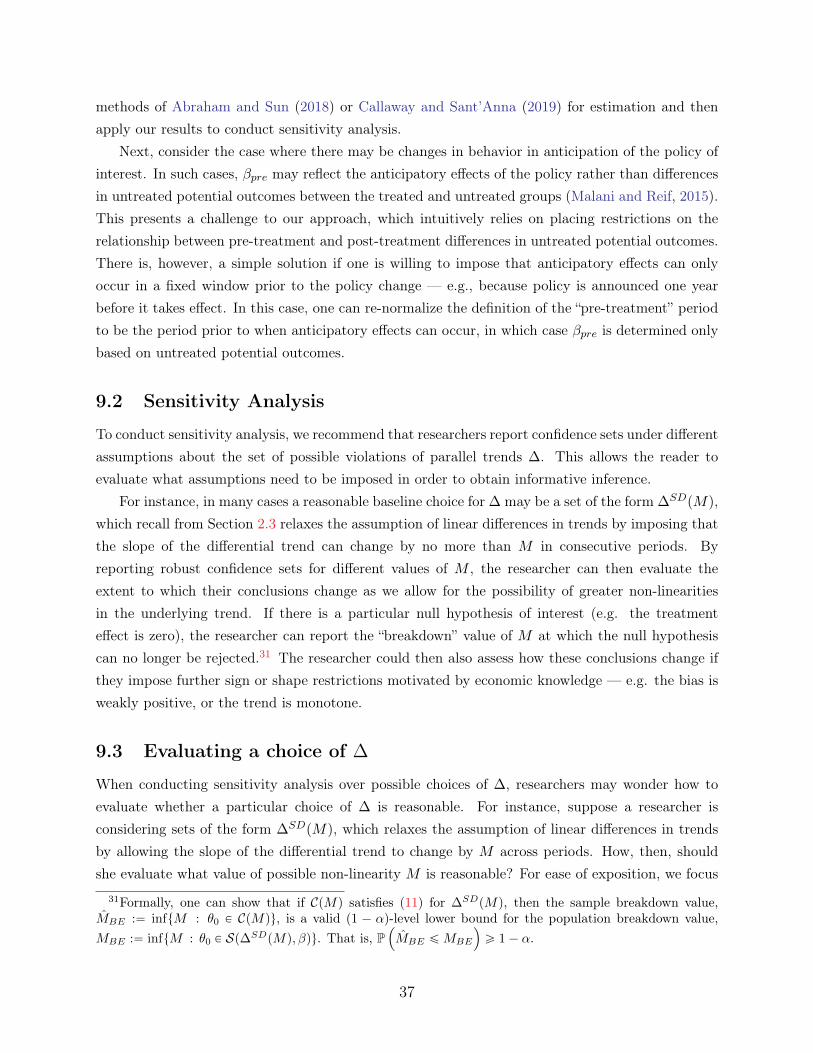
methods of Abraham and Sun (2018) or Callaway and Sant’Anna (2019) for estimation and thenapply our results to conduct sensitivity analysis.

Next, consider the case where there may be changes in behavior in anticipation of the policy ofinterest. In such cases, βpre may reflect the anticipatory effects of the policy rather than differencesin untreated potential outcomes between the treated and untreated groups (Malani and Reif, 2015).This presents a challenge to our approach, which intuitively relies on placing restrictions on therelationship between pre-treatment and post-treatment differences in untreated potential outcomes.There is, however, a simple solution if one is willing to impose that anticipatory effects can onlyoccur in a fixed window prior to the policy change — e.g., because policy is announced one yearbefore it takes effect. In this case, one can re-normalize the definition of the “pre-treatment” periodto be the period prior to when anticipatory effects can occur, in which case βpre is determined onlybased on untreated potential outcomes.

9.2 Sensitivity Analysis

To conduct sensitivity analysis, we recommend that researchers report confidence sets under differentassumptions about the set of possible violations of parallel trends ∆. This allows the reader toevaluate what assumptions need to be imposed in order to obtain informative inference.

For instance, in many cases a reasonable baseline choice for ∆ may be a set of the form ∆SDpMq,which recall from Section 2.3 relaxes the assumption of linear differences in trends by imposing thatthe slope of the differential trend can change by no more than M in consecutive periods. Byreporting robust confidence sets for different values of M , the researcher can then evaluate theextent to which their conclusions change as we allow for the possibility of greater non-linearitiesin the underlying trend. If there is a particular null hypothesis of interest (e.g. the treatmenteffect is zero), the researcher can report the “breakdown” value of M at which the null hypothesiscan no longer be rejected.31 The researcher could then also assess how these conclusions change ifthey impose further sign or shape restrictions motivated by economic knowledge — e.g. the bias isweakly positive, or the trend is monotone.

9.3 Evaluating a choice of ∆

When conducting sensitivity analysis over possible choices of ∆, researchers may wonder how toevaluate whether a particular choice of ∆ is reasonable. For instance, suppose a researcher isconsidering sets of the form ∆SDpMq, which relaxes the assumption of linear differences in trendsby allowing the slope of the differential trend to change by M across periods. How, then, shouldshe evaluate what value of possible non-linearity M is reasonable? For ease of exposition, we focus

31Formally, one can show that if CpMq satisfies (11) for ∆SDpMq, then the sample breakdown value,MBE :“ inftM : θ0 P CpMqu, is a valid p1 ´ αq-level lower bound for the population breakdown value,MBE :“ inftM : θ0 P Sp∆SDpMq, βqu. That is, P

´

MBE ďMBE

¯

ě 1´ α.

37

on how to evaluate M in this case, although analogous remarks apply to conducting sensitivity forother forms of ∆ as well.

We stress that nothing in the data itself can place an upper bound on the parameter M . This isbecauseM places limits on the possible non-linearity in the counterfactual difference in trends δpost,which is not identified from the data. Researchers therefore must use domain-specific knowledgeto evaluate whether a particular choice of M is plausible in a given empirical setting. To helpresearchers do so, we discuss two approaches that benchmark possible values of M using knowledgeof potential confounds and using untreated groups or periods. These benchmarking exercises may beuseful in calibrating the restrictiveness of a particular set of assumptions about the counterfactualdifference in trends.

Benchmarking using knowledge of potential confounds. One way to calibrate M is toconsider the types of mechanisms which may produce a violation of parallel trends, and to benchmarkM using knowledge of the likely magnitudes of those mechanisms. We provide an example of thistype of reasoning in our application to Lovenheim and Willen (2019) in Section 10. In that setting,there are concerns that differential changes in education quality across states may produce non-parallel trends in employment outcomes, and we benchmark the magnitude of such changes usingestimates of the effects of teacher value-added on employment outcomes from Chetty, Friedman andRockoff (2014). This suggestion echoes Kahn-Lang and Lang (2018), who advocate for the use ofdomain-specific knowledge in justifying the parallel trends assumption. �

Benchmarking using untreated groups or periods. In some settings, researchers mayhave a set of untreated (placebo) groups who they think are “at least as dissimilar” as the groupsused in their main analysis. In this case, it may be sensible to form a confidence interval for thelargest change in slope between periods among the placebo groups, and use the upper bound ofthat interval as a benchmark for M .32 This allows researchers to make statements of the form, “wecan reject the null hypothesis unless we allow for changes in slope more than X times as large asthe upper bound for the largest change observed for the placebo groups.” Along similar lines, onecould also construct an upper bound on the largest change in slope in the pre-period for the groupsused in the main event-study of interest. One could then benchmark M in terms of multiples of the

32A simple way of forming such an interval is as follows: Let βplacebo be the vector of estimated event-study coefficients for the placebo groups, and δplacebo its expectation. We wish to form a lower one-sidedCI for Mplacebo :“ maxjpA

SDδplaceboqj , where ASD is the matrix that creates second differences. Letubj “ pA

SDβplaceboqj `σjz1´α be the upper bound of a standard one-sided confidence interval for the meanof pASDβplaceboqj , where σj is the standard deviation of pASDβplaceboqj . Define ub :“ maxj ubj . Thenp´8, ubs is a level p1´αq CI forMplacebo. Proper coverage of this CI follows from results by Berger and Hsu(1996) on the “union-intersection” approach, since H0 : Mplacebo ě m is equivalent to H0 : E

”

ASDβplaceboı

PŤ

jtµ : µj ě mu.

38

largest value observed in the pre-period.33 �

We note that while an upper bound on the parameter M may not be learned from the data, theobserved pre-period data can possibly provide an informative lower bound on possible values of M .We now discuss how such a bound can be constructed, and how it should (and should not) be used.

Lower bounding M . Recall that M is an upper limit on how much the slope of δ can changebetween periods. Thus, the largest second difference in δpre must be no larger than M in absolutevalue. Since δpre is the expected value of the pre-period coefficients βpre, we can test this hypothesisusing the pre-period coefficients. In particular, we can reject a value of M if we reject the nullhypothesis H0 : E

”

ASDβpre

ı

ď M , where ASD is the matrix that produces the positive and

negative second differences of βpre. This is again a test of a system of moment inequalities, and canbe tested using the conditional test described in Section 4.34

This exercise is a sensible approach to test whether a given value of M is rejected by the data,and researchers should be skeptical of confidence sets relying on small values of M that are stronglyrejected by the data. We caution, however, that this exercise provides only a lower bound on thepossible value of M . The fact that the pre-period second differences in δ are small does not on itsown place a bound on how large the second differences in the post-period could have been under thecounterfactual. Thus, if a small value of M is not rejected by the data, we should not necessarilyconclude that it is reasonable. We specifically caution against concluding that M “ 0 (i.e. linearviolations of parallel trends) is reasonable simply because it cannot be rejected by the data. Wefurther note that relying on such tests raises standard concerns associated with pre-testing.

9.4 Choice of Confidence Sets and Computation

As discussed in detail in Section 8.3, we recommend that researchers select either the optimal FLCIor a hybridized conditional confidence set based upon the properties of their specified choice of ∆.For special cases (e.g. ∆ “ ∆SDpMq) where the conditions for the consistency of the FLCIs arenon-restrictive and the conditions for finite-sample near-optimality under parallel trends hold, werecommend that the researchers use the optimal FLCI. Otherwise, we recommend that researchersuse a hybrid confidence set that hybridizes the conditional approach with the optimal FLCI or with

33We view the exercise of upper-bounding the largest change in the pre-period slope (Mpre) as a way ofcasting the assumption that ∆ “ ∆SDpMq in easily-interpretable units. If one instead wants to use thisas the basis of an identifying assumption (i.e. assuming that the post-period change in slope is no largerthan the largest pre-period change), then a tractable method for obtaining valid inference over the implied∆ is to first form a level 1´ α{2 upper bound on Mpre, say Mub

pre, and then estimate a robust 1´ α{2 levelconfidence set using ∆SDpMub

preq.34More generally, the null H0 : δ P ∆ “ tδ : Aδ ď du is equivalent to H0 :

Dτpost s.t. E”

Apβ ´Mpostτpostq ´ dı

ď 0, which can be tested using the conditional test, or the conditional-LF test described in the Appendix.

39

a least-favorable test. These confidence sets are all quick and straightforward to compute. Forexample, each of the sensitivity analysis plots in Section 10 take less than 10 minutes to produceon a 2014 Macbook Pro. Our R package HonestDiD by default chooses our recommended methoddepending on the specified choice of ∆, but allows the user to override these defaults.

10 Empirical Applications

We now apply our methods to two recently published papers. In doing so, we illustrate how empiricalresearchers can use our methods to conduct formal sensitivity analyses in difference-in-differencesand event-study designs.

10.1 The effect of duty-to-bargain laws on long-run student out-

comes

We first apply our results to the analysis of the effects of teacher collective bargaining on long-runstudent outcomes in Lovenheim and Willen (2019, henceforth LW).

LW study the impact of state-level public sector duty-to-bargain (DTB) laws, which mandatedthat school districts bargain in good faith with teachers’ unions. The majority of these laws werepassed in the 1960s-1980s. LW use data from the American Community Survey (ACS) from 2005-2012 to examine the impacts of these laws on the adult labor market outcomes of people whowere students around the time that these laws were passed. Their identification strategy comparesindividuals across different states and different birth cohorts to exploit the differential timing ofthe passage of DTB laws across states. In particular, the authors estimate the following regressionspecification separately for men and women,

Ysct “21ÿ

r“´11

Dscrβr `X1sctγ ` λct ` φs ` εsct. (28)

Ysct is an average outcome for the cohort of students born in state s in cohort c in ACS calendaryear t. Dscr is an indicator for whether state s passed a DTB law r years before cohort c turned age18.35 Thus, the coefficients tβru estimate the dynamic treatment effect (or placebo effect) r yearsafter DTB passage. The remaining terms in the regression are time-varying controls, birth-cohort-by-ACS-year fixed effects, and state fixed effects. Standard errors are clustered at the state level,and we normalize the coefficient β´2 to 0.36

35Dsc,´11 is set to 1 if state s passed a law 11 years or more after cohort c turned 18. Likewise, Dsc,21 isset to 1 if state s passed a law 21 or more years before cohort c turned 18.

36LW normalize event time -1 to 0, but discuss how cohorts at event time -1 may have been partiallytreated, since LW impute the year that a student starts school with error. Since our robust confidence setsassume that there is no causal effect in the pre-period (τpre “ 0), we instead treat event-time -2 as the

40

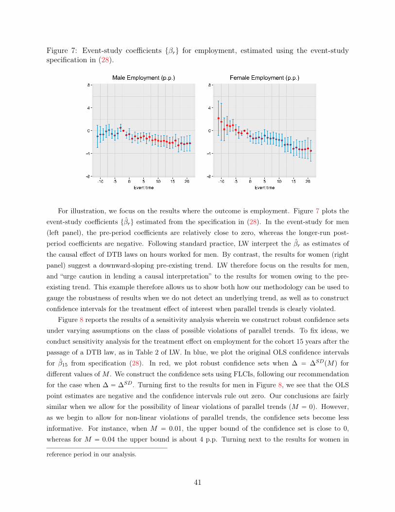
Figure 7: Event-study coefficients tβru for employment, estimated using the event-studyspecification in (28).

For illustration, we focus on the results where the outcome is employment. Figure 7 plots theevent-study coefficients tβru estimated from the specification in (28). In the event-study for men(left panel), the pre-period coefficients are relatively close to zero, whereas the longer-run post-period coefficients are negative. Following standard practice, LW interpret the βr as estimates ofthe causal effect of DTB laws on hours worked for men. By contrast, the results for women (rightpanel) suggest a downward-sloping pre-existing trend. LW therefore focus on the results for men,and “urge caution in lending a causal interpretation” to the results for women owing to the pre-existing trend. This example therefore allows us to show both how our methodology can be used togauge the robustness of results when we do not detect an underlying trend, as well as to constructconfidence intervals for the treatment effect of interest when parallel trends is clearly violated.

Figure 8 reports the results of a sensitivity analysis wherein we construct robust confidence setsunder varying assumptions on the class of possible violations of parallel trends. To fix ideas, weconduct sensitivity analysis for the treatment effect on employment for the cohort 15 years after thepassage of a DTB law, as in Table 2 of LW. In blue, we plot the original OLS confidence intervalsfor β15 from specification (28). In red, we plot robust confidence sets when ∆ “ ∆SDpMq fordifferent values ofM . We construct the confidence sets using FLCIs, following our recommendationfor the case when ∆ “ ∆SD. Turning first to the results for men in Figure 8, we see that the OLSpoint estimates are negative and the confidence intervals rule out zero. Our conclusions are fairlysimilar when we allow for the possibility of linear violations of parallel trends (M “ 0). However,as we begin to allow for non-linear violations of parallel trends, the confidence sets become lessinformative. For instance, when M “ 0.01, the upper bound of the confidence set is close to 0,whereas for M “ 0.04 the upper bound is about 4 p.p. Turning next to the results for women in

reference period in our analysis.

41

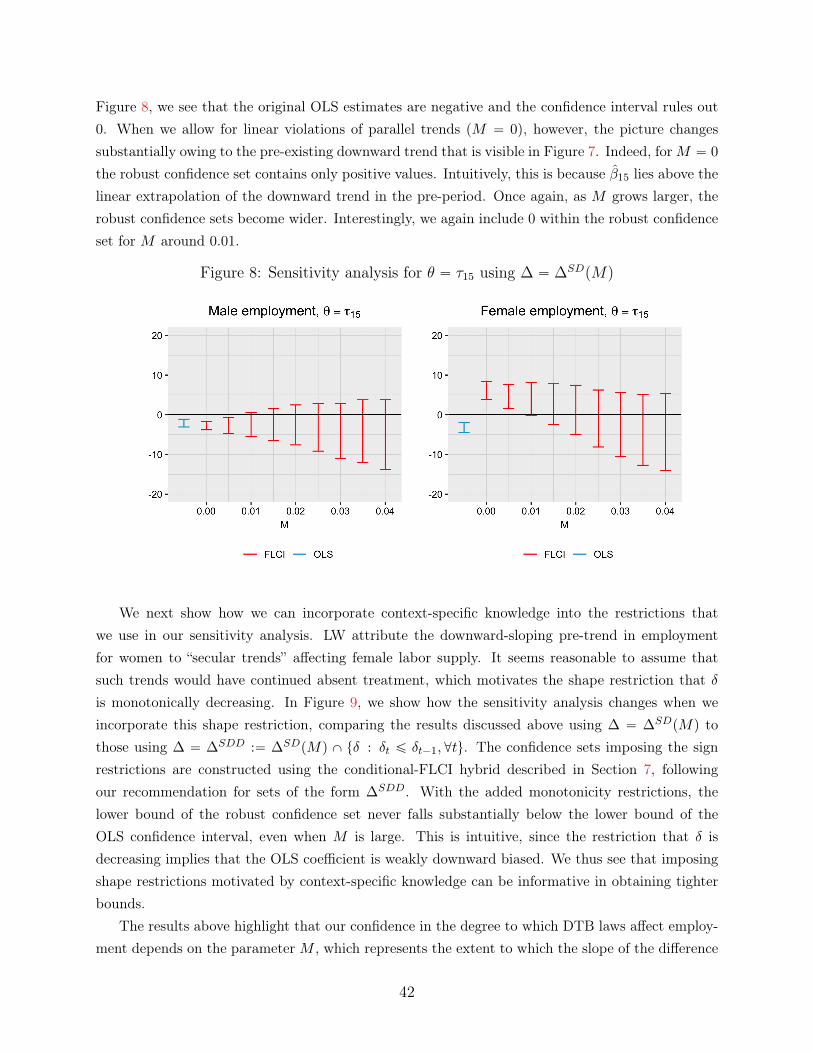
Figure 8, we see that the original OLS estimates are negative and the confidence interval rules out0. When we allow for linear violations of parallel trends pM “ 0q, however, the picture changessubstantially owing to the pre-existing downward trend that is visible in Figure 7. Indeed, forM “ 0

the robust confidence set contains only positive values. Intuitively, this is because β15 lies above thelinear extrapolation of the downward trend in the pre-period. Once again, as M grows larger, therobust confidence sets become wider. Interestingly, we again include 0 within the robust confidenceset for M around 0.01.

Figure 8: Sensitivity analysis for θ “ τ15 using ∆ “ ∆SDpMq

We next show how we can incorporate context-specific knowledge into the restrictions thatwe use in our sensitivity analysis. LW attribute the downward-sloping pre-trend in employmentfor women to “secular trends” affecting female labor supply. It seems reasonable to assume thatsuch trends would have continued absent treatment, which motivates the shape restriction that δis monotonically decreasing. In Figure 9, we show how the sensitivity analysis changes when weincorporate this shape restriction, comparing the results discussed above using ∆ “ ∆SDpMq tothose using ∆ “ ∆SDD :“ ∆SDpMq X tδ : δt ď δt´1,@tu. The confidence sets imposing the signrestrictions are constructed using the conditional-FLCI hybrid described in Section 7, followingour recommendation for sets of the form ∆SDD. With the added monotonicity restrictions, thelower bound of the robust confidence set never falls substantially below the lower bound of theOLS confidence interval, even when M is large. This is intuitive, since the restriction that δ isdecreasing implies that the OLS coefficient is weakly downward biased. We thus see that imposingshape restrictions motivated by context-specific knowledge can be informative in obtaining tighterbounds.

The results above highlight that our confidence in the degree to which DTB laws affect employ-ment depends on the parameter M , which represents the extent to which the slope of the difference

42

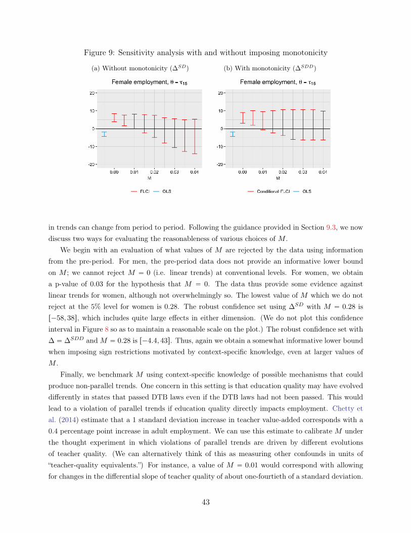
Figure 9: Sensitivity analysis with and without imposing monotonicity

(a) Without monotonicity (∆SDq (b) With monotonicity (∆SDDq

in trends can change from period to period. Following the guidance provided in Section 9.3, we nowdiscuss two ways for evaluating the reasonableness of various choices of M .

We begin with an evaluation of what values of M are rejected by the data using informationfrom the pre-period. For men, the pre-period data does not provide an informative lower boundon M ; we cannot reject M “ 0 (i.e. linear trends) at conventional levels. For women, we obtaina p-value of 0.03 for the hypothesis that M “ 0. The data thus provide some evidence againstlinear trends for women, although not overwhelmingly so. The lowest value of M which we do notreject at the 5% level for women is 0.28. The robust confidence set using ∆SD with M “ 0.28 isr´58, 38s, which includes quite large effects in either dimension. (We do not plot this confidenceinterval in Figure 8 so as to maintain a reasonable scale on the plot.) The robust confidence set with∆ “ ∆SDD andM “ 0.28 is r´4.4, 43s. Thus, again we obtain a somewhat informative lower boundwhen imposing sign restrictions motivated by context-specific knowledge, even at larger values ofM .

Finally, we benchmark M using context-specific knowledge of possible mechanisms that couldproduce non-parallel trends. One concern in this setting is that education quality may have evolveddifferently in states that passed DTB laws even if the DTB laws had not been passed. This wouldlead to a violation of parallel trends if education quality directly impacts employment. Chetty etal. (2014) estimate that a 1 standard deviation increase in teacher value-added corresponds with a0.4 percentage point increase in adult employment. We can use this estimate to calibrate M underthe thought experiment in which violations of parallel trends are driven by different evolutionsof teacher quality. (We can alternatively think of this as measuring other confounds in units of“teacher-quality equivalents.”) For instance, a value of M “ 0.01 would correspond with allowingfor changes in the differential slope of teacher quality of about one-fourtieth of a standard deviation.

43

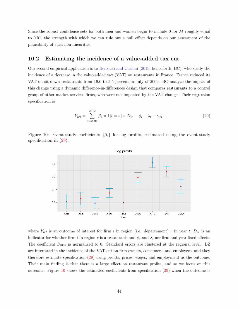
Since the robust confidence sets for both men and women begin to include 0 for M roughly equalto 0.01, the strength with which we can rule out a null effect depends on our assessment of theplausibility of such non-linearities.

10.2 Estimating the incidence of a value-added tax cut

Our second empirical application is to Benzarti and Carloni (2019, henceforth, BC), who study theincidence of a decrease in the value-added tax (VAT) on restaurants in France. France reduced itsVAT on sit-down restaurants from 19.6 to 5.5 percent in July of 2009. BC analyze the impact ofthis change using a dynamic difference-in-differences design that compares restaurants to a controlgroup of other market services firms, who were not impacted by the VAT change. Their regressionspecification is

Yirt “2012ÿ

s“2004

βs ˆ 1rt “ ss ˆDir ` φi ` λt ` εirt, (29)

Figure 10: Event-study coefficients tβsu for log profits, estimated using the event-studyspecification in (29).

where Yirt is an outcome of interest for firm i in region (i.e. département) r in year t; Dir is anindicator for whether firm i in region r is a restaurant; and φi and λt are firm and year fixed effects.The coefficient β2008 is normalized to 0. Standard errors are clustered at the regional level. BZare interested in the incidence of the VAT cut on firm owners, consumers, and employees, and theytherefore estimate specification (29) using profits, prices, wages, and employment as the outcome.Their main finding is that there is a large effect on restaurant profits, and so we focus on thisoutcome. Figure 10 shows the estimated coefficients from specification (29) when the outcome is

44

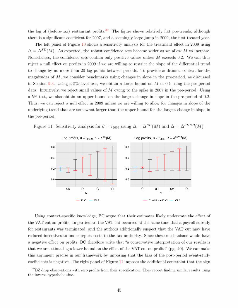
the log of (before-tax) restaurant profits.37 The figure shows relatively flat pre-trends, althoughthere is a significant coefficient for 2007, and a seemingly large jump in 2009, the first treated year.

The left panel of Figure 10 shows a sensitivity analysis for the treatment effect in 2009 using∆ “ ∆SDpMq. As expected, the robust confidence sets become wider as we allow M to increase.Nonetheless, the confidence sets contain only positive values unless M exceeds 0.2. We can thusreject a null effect on profits in 2009 if we are willing to restrict the slope of the differential trendto change by no more than 20 log points between periods. To provide additional context for themagnitudes of M , we consider benchmarks using changes in slope in the pre-period, as discussedin Section 9.3. Using a 5% level test, we obtain a lower bound on M of 0.1 using the pre-perioddata. Intuitively, we reject small values of M owing to the spike in 2007 in the pre-period. Usinga 5% test, we also obtain an upper bound on the largest change in slope in the pre-period of 0.2.Thus, we can reject a null effect in 2009 unless we are willing to allow for changes in slope of theunderlying trend that are somewhat larger than the upper bound for the largest change in slope inthe pre-period.

Figure 11: Sensitivity analysis for θ “ τ2009 using ∆ “ ∆SDpMq and ∆ “ ∆SDNBpMq.

Using context-specific knowledge, BC argue that their estimates likely understate the effect ofthe VAT cut on profits. In particular, the VAT cut occurred at the same time that a payroll subsidyfor restaurants was terminated, and the authors additionally suspect that the VAT cut may havereduced incentives to under-report costs to the tax authority. Since these mechanisms would havea negative effect on profits, BC therefore write that “a conservative interpretation of our results isthat we are estimating a lower bound on the effect of the VAT cut on profits” (pg. 40). We can makethis argument precise in our framework by imposing that the bias of the post-period event-studycoefficients is negative. The right panel of Figure 11 imposes the additional constraint that the sign

37BZ drop observations with zero profits from their specification. They report finding similar results usingthe inverse hyperbolic sine.

45

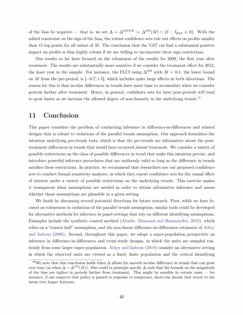
of the bias be negative — that is, we set ∆ “ ∆SDNB :“ ∆SDpMq X tδ : δpost ď 0u. With theadded constraint on the sign of the bias, the robust confidence sets rule out effects on profits smallerthan 15 log points for all values of M . The conclusion that the VAT cut had a substantial positiveimpact on profits is thus highly robust if we are willing to incorporate these sign restrictions.

Our results so far have focused on the robustness of the results for 2009, the first year aftertreatment. The results are substantially more sensitive if we consider the treatment effect for 2012,the least year in the sample. For instance, the FLCI using ∆SD with M “ 0.1, the lower boundon M from the pre-period, is r´0.7, 1.5s, which includes quite large effects in both directions. Thereason for this is that secular differences in trends have more time to accumulate when we considerperiods farther after treatment. Hence, in general, confidence sets for later post-periods will tendto grow faster as we increase the allowed degree of non-linearity in the underlying trends.38

11 Conclusion

This paper considers the problem of conducting inference in difference-in-differences and relateddesigns that is robust to violations of the parallel trends assumption. Our approach formalizes theintuition underlying pre-trends tests, which is that the pre-trends are informative about the post-treatment differences in trends that would have occurred absent treatment. We consider a variety ofpossible restrictions on the class of possible differences in trend that make this intuition precise, andintroduce powerful inference procedures that are uniformly valid so long as the difference in trendssatisfies these restrictions. In practice, we recommend that researchers use our proposed confidencesets to conduct formal sensitivity analyses, in which they report confidence sets for the causal effectof interest under a variety of possible restrictions on the underlying trends. This exercise makesit transparent what assumptions are needed in order to obtain informative inference and assesswhether those assumptions are plausible in a given setting.

We finish by discussing several potential directions for future research. First, while we have fo-cused on robustness to violations of the parallel trends assumption, similar tools could be developedfor alternative methods for inference in panel settings that rely on different identifying assumptions.Examples include the synthetic control method (Abadie, Diamond and Hainmueller, 2010), whichrelies on a “convex hull” assumption, and the non-linear difference-in-differences estimator of Atheyand Imbens (2006). Second, throughout this paper, we adopt a super-population perspective oninference in difference-in-differences and event-study designs, in which the units are sampled ran-domly from some larger super-population. Athey and Imbens (2018) consider an alternative settingin which the observed units are viewed as a fixed, finite population and the critical identifying

38We note that this conclusion holds when ∆ allows for smooth secular difference in trends that can growover time (as when ∆ “ ∆SDpMq). One could in principle specify ∆ such that the bounds on the magnitudeof the bias are tighter in periods farther from treatment. This might be sensible in certain cases — forinstance, if one suspects that policy is passed in response to temporary, short-run shocks that revert to themean over longer horizons.

46

assumption is that the timing of treatment is completely random. An interesting open questionis how to conduct inference that is robust to possible non-random treatment timing in this finite-population setting. Finally, pre-trends testing is but one example of the wide use of placebo testingin quasi-experimental research designs. Similar methods could potentially be extended to conductrobust inference in other types of quasi-experimental research designs.

ReferencesAbadie, Alberto, “Semiparametric Difference-in-Differences Estimators,” The Review of Economic

Studies, 2005, 72 (1), 1–19.

, Alexis Diamond, and Jens Hainmueller, “Synthetic Control Methods for ComparativeCase Studies: Estimating the Effect of California’s Tobacco Control Program,” Journal of theAmerican Statistical Association, June 2010, 105 (490), 493–505.

and Guido W. Imbens, “Large Sample Properties of Matching Estimators for Average Treat-ment Effects,” Econometrica, 2006, 74 (1), 235–267.

Abraham, Sarah and Liyang Sun, “Estimating Dynamic Treatment Effects in Event StudiesWith Heterogeneous Treatment Effects,” SSRN Scholarly Paper ID 3158747, Social Science Re-search Network, Rochester, NY April 2018.

Altonji, Joseph G., Todd E. Elder, and Christopher R. Taber, “Selection on Observedand Unobserved Variables: Assessing the Effectiveness of Catholic Schools,” Journal of PoliticalEconomy, 2005, 113 (1), 151–184.

Andrews, DonaldW. K. and Panle Jia Barwick, “Inference for Parameters Defined by MomentInequalities: A Recommended Moment Selection Procedure,” Econometrica, 2012, 80 (6), 2805–2826.

Andrews, Donald, Xu Cheng, and Patrik Guggenberger, “Generic Results for Establishingthe Asymptotic Size of Confidence Sets and Tests,” Journal of Econometrics, Forthcoming.

Andrews, Isaiah, Jonathan Roth, and Ariel Pakes, “Inference for Linear Conditional MomentInequalities,” Working Paper 2019.

, Matthew Gentzkow, and Jesse Shapiro, “Measuring the Sensitivity of Parameter Estimatesto Estimation Moments,” The Quarterly Journal of Economics, 2017, 132 (4), 1553–1592.

, , and , “On the Informativeness of Descriptive Statistics for Structural Estimates,” Tech-nical Report 2019.

Angrist, Joshua D. and Jorn-Steffen Pischke, Mostly Harmless Econometrics: An Empiricist’sCompanion, Princeton: Princeton University Press, 2009.

Arellano, Manuel, “Computing robust standard errors for within-groups estimators,” Oxford Bul-letin of Economics and Statistics, 1987, 49 (4), 431–434.

Armstrong, Timothy and Michal Kolesar, “Optimal Inference in a Class of Regression Models,”Econometrica, 2018, 86, 655–683.

47

and , “Sensitivity Analysis using Approximate Moment Condition Models,” Technical Report2019.

Ashenfelter, Orley, “Estimating the Effect of Training Programs on Earnings,” The Review ofEconomics and Statistics, 1978, 60 (1), 47–57.

Athey, Susan and Guido Imbens, “Design-Based Analysis in Difference-In-Differences Settingswith Staggered Adoption,” arXiv:1808.05293 [cs, econ, math, stat], August 2018.

and Guido W. Imbens, “Identification and Inference in Nonlinear Difference-in-DifferencesModels,” Econometrica, 2006, 74 (2), 431–497.

Balke, Alexander and Judea Pearl, “Bounds on Treatment Effects from Studies with ImperfectCompliance,” Journal of the American Statistical Association, 1997, 92 (439), 1171–1176.

Benzarti, Youssef and Dorian Carloni, “Who Really Benefits from Consumption Tax Cuts?Evidence from a Large VAT Reform in France,” American Economic Journal: Economic Policy,February 2019, 11 (1), 38–63.

Berger, Roger L. and Jason C. Hsu, “Bioequivalence trials, intersection-union tests and equiv-alence confidence sets,” Statistical Science, November 1996, 11 (4), 283–319.

Bertrand, Marianne, Esther Duflo, and Sendhil Mullainathan, “HowMuch ShouldWe TrustDifferences-In-Differences Estimates?,” The Quarterly Journal of Economics, February 2004, 119(1), 249–275.

Bhattacharya, Jay, Azeem M. Shaikh, and Edward Vytlacil, “Treatment Effect Boundsunder Monotonicity Assumptions: An Application to Swan-Ganz Catheterization,” AmericanEconomic Review, May 2008, 98 (2), 351–356.

Bhuller, Manudeep, Tarjei Havnes, Edwin Leuven, and Magne Mogstad, “BroadbandInternet: An Information Superhighway to Sex Crime?,” The Review of Economics and Statistics,2013, 80, 1237—-1266.

Bilinski, Alyssa and Laura A. Hatfield, “Seeking Evidence of Absence: Reconsidering Tests ofModel Assumptions,” arXiv:1805.03273 [stat], May 2018.

Bonhomme, Stephanne and Martin Weidner, “Minimizing Sensitivity to Model Misspecifica-tion,” Technical Report 2018.

Borusyak, Kirill and Xavier Jaravel, “Revisiting Event Study Designs,” SSRN Scholarly PaperID 2826228, Social Science Research Network, Rochester, NY August 2016.

Bugni, Federico A., Ivan A. Canay, and Xiaoxia Shi, “Inference for subvectors and other func-tions of partially identified parameters in moment inequality models,” Quantitative Economics,2017, 8 (1), 1–38.

Callaway, Brantly and Pedro H. C. Sant’Anna, “Difference-in-Differences with Multiple TimePeriods,” SSRN Scholarly Paper ID 3148250, Social Science Research Network, Rochester, NYMarch 2019.

48

Canay, Ivan and Azeem Shaikh, “Practical and Theoretical Advances in Inference for PartiallyIdentified Models,” in Bo Honoré, Ariel Pakes, Monika Piazzesi, and Larry Samuelson, eds.,Advances in Economics and Econometrics, 2017, pp. 271–306.

Chen, Xiaohong, Timothy M. Christensen, and Elie Tamer, “Monte Carlo Confidence Setsfor Identified Sets,” Econometrica, 2018, 86 (6), 1965–2018.

Chernozhukov, Victor, Whitney K. Newey, and Andres Santos, “Constrained ConditionalMoment Restriction Models,” arXiv:1509.06311 [math, stat], September 2015. arXiv: 1509.06311.

Chetty, Raj, John N. Friedman, and Jonah E. Rockoff, “Measuring the Impacts of TeachersII: Teacher Value-Added and Student Outcomes in Adulthood,” American Economic Review,September 2014, 104 (9), 2633–2679.

Cho, JoonHwan and Thomas M. Russell, “Simple Inference on Functionals of Set-IdentifiedParameters Defined by Linear Moments,” October 2018.

Christensen, Timothy and Benjamin Connault, “Counterfactual Sensitivity and Robustness,”arXiv:1904.00989 [econ], April 2019. arXiv: 1904.00989.

Conley, Timothy, Christian Hansen, and Peter Rossi, “Plausibly Exogenous,” The Reviewof Economics and Statistics, 2012, 94 (1), 260–272.

Conley, Timothy G. and Christopher R. Taber, “Inference with “Difference in Differences”with a Small Number of Policy Changes,” The Review of Economics and Statistics, July 2010, 93(1), 113–125.

Cox, Gregory and Xiaoxia Shi, “A Simple Uniformly Valid Test for Inequalities,”arXiv:1907.06317 [econ, math, stat], July 2019. arXiv: 1907.06317.

Cunningham, Scott, Causal Inference: The Mixtape, Unpublished manuscript, 2018.

de Chaisemartin, Clément and Xavier D’Haultfœuille, “Fuzzy Differences-in-Differences,”The Review of Economic Studies, April 2018, 85 (2), 999–1028.

and , “Two-way fixed effects estimators with heterogeneous treatment effects,”arXiv:1803.08807 [econ], March 2018. arXiv: 1803.08807.

Ding, Peng and Tyler J. VanderWeele, “Sensitivity Analysis without Assumptions,” Epidemi-ology, 2016, 27 (3), 368–377.

Dobkin, Carlos, Amy Finkelstein, Raymond Kluender, and Matthew J. Notowidigdo,“The Economic Consequences of Hospital Admissions,” 2018, 108 (2), 308–352.

Donald, Stephen G. and Kevin Lang, “Inference with Difference-in-Differences and Other PanelData,” The Review of Economics and Statistics, 2007, 89 (2), 221–233.

Donoho, David L., “Statistical Estimation and Optimal Recovery,” The Annals of Statistics, 1994,22 (1), 238–270.

Ferman, Bruno and Cristine Pinto, “Inference in Differences-in-Differences with Few TreatedGroups and Heteroskedasticity,” The Review of Economics and Statistics, July 2018, 101 (3),452–467.

49

Flynn, Zach, “Inference Based on Continuous Linear Inequalities via Semi-Infinite Programming,”SSRN Scholarly Paper ID 3390788, Social Science Research Network, Rochester, NY May 2019.

Frandsen, Brigham R, “The Effects of Collective Bargaining Rights on Public Employee Com-pensation: Evidence from Teachers, Firefighters, and Police,” ILR Review, 2016, 69 (1), 84–112.

Freyaldenhoven, Simon, Christian Hansen, and Jesse Shapiro, “Pre-event Trends in thePanel Event-study Design,” American Economic Review, 2019, 109 (9), 3307–3338.

Gafarov, Bulat, “Inference in high-dimensional set-identified affine models,” March 2019.

Ginther, Donna K., “Alternative Estimates of the Effect of Schooling on Earnings,” The Reviewof Economics and Statistics, February 2000, 82 (1), 103–116.

González, Libertad, “Nonparametric bounds on the returns to language skills,” Journal of AppliedEconometrics, 2005, 20 (6), 771–795.

Goodman-Bacon, Andrew, “Difference-in-Differences with Variation in Treatment Timing,”Working Paper 25018, National Bureau of Economic Research September 2018.

, “Public Insurance and Mortality: Evidence from Medicaid Implementation,” Journal of PublicEconomics, 2018, 126 (1), 216–262.

Greenstone, Michael and Rema Hanna, “Environmental Regulations, Air and Water Pollution,and Infant Mortality in India,” American Economic Review, October 2014, 104 (10), 3038–3072.

Gunsilius, Florian, “Bounds in continuous instrumental variable models,” Technical Report 2019.

Heckman, James, Hidehiko Ichimura, Jeffrey Smith, and Petra Todd, “CharacterizingSelection Bias Using Experimental Data,” Econometrica, 1998, 66 (5), 1017–1098.

Heckman, James J. and Edward J. Vytlacil, “Local instrumental variables and latent variablemodels for identifying and bounding treatment effects,” Proceedings of the National Academy ofSciences, April 1999, 96 (8), 4730.

Ho, Kate and Adam Rosen, “Partial Identification in Applied Research: Benefits and Chal-lenges,” in Bo Honoré, Ariel Pakes, Monika Piazzesi, and Larry Samuelson, eds., Advances inEconomics and Econometrics, 2017, pp. 307–359.

Horowitz, Joel L. and Charles F. Manski, “Identification and Robustness with Contaminatedand Corrupted Data,” Econometrica, 1995, 63 (2), 281–302.

Hudson, Sally, Peter Hull, and Jack Liebersohn, “Interpreting Instrumented Difference-in-Differences,” Working Paper 2017.

Hull, Peter, “Estimating Treatment Effects in Movers Designs,” Technical Report 2018.

Imai, Kosuke and In Song Kim, “On the Use of Two-way Fixed Effects Regression Models forCausal Inference with Panel Data,” 2019.

Imbens, Guido, “Sensitivity to Exogeneity Assumptions in Program Evaluation,” American Eco-nomic Review, 2003, 93 (2), 126–132.

50

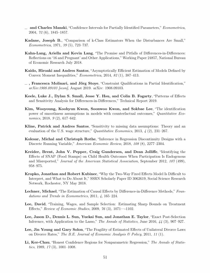
and Charles Manski, “Confidence Intervals for Partially Identified Parameters,” Econometrica,2004, 72 (6), 1845–1857.

Kadane, Joseph B., “Comparison of k-Class Estimators When the Disturbances Are Small,”Econometrica, 1971, 39 (5), 723–737.

Kahn-Lang, Ariella and Kevin Lang, “The Promise and Pitfalls of Differences-in-Differences:Reflections on ‘16 and Pregnant’ and Other Applications,” Working Paper 24857, National Bureauof Economic Research July 2018.

Kaido, Hiroaki and Andres Santos, “Asymptotically Efficient Estimation of Models Defined byConvex Moment Inequalities,” Econometrica, 2014, 82 (1), 387–413.

, Francesca Molinari, and Jörg Stoye, “Constraint Qualifications in Partial Identification,”arXiv:1908.09103 [econ], August 2019. arXiv: 1908.09103.

Keele, Luke J., Dylan S. Small, Jesse Y. Hsu, and Colin B. Fogarty, “Patterns of Effectsand Sensitivity Analysis for Differences-in-Differences,” Technical Report 2019.

Kim, Wooyoung, Koohyun Kwon, Soonwoo Kwon, and Sokbae Lee, “The identificationpower of smoothness assumptions in models with counterfactual outcomes,” Quantitative Eco-nomics, 2018, 9 (2), 617–642.

Kline, Patrick and Andres Santos, “Sensitivity to missing data assumptions: Theory and anevaluation of the U.S. wage structure,” Quantitative Economics, 2013, 4 (2), 231–267.

Kolesar, Michal and Christoph Rothe, “Inference in Regression Discontinuity Designs with aDiscrete Running Variable,” American Economic Review, 2018, 108 (8), 2277–2304.

Kreider, Brent, John V. Pepper, Craig Gundersen, and Dean Jolliffe, “Identifying theEffects of SNAP (Food Stamps) on Child Health Outcomes When Participation Is Endogenousand Misreported,” Journal of the American Statistical Association, September 2012, 107 (499),958–975.

Kropko, Jonathan and Robert Kubinec, “Why the Two-Way Fixed Effects Model Is Difficult toInterpret, and What to Do About It,” SSRN Scholarly Paper ID 3062619, Social Science ResearchNetwork, Rochester, NY May 2018.

Lechner, Michael, “The Estimation of Causal Effects by Difference-in-Difference Methods,” Foun-dations and Trends in Econometrics, 2011, 4, 165–224.

Lee, David, “Training, Wages, and Sample Selection: Estimating Sharp Bounds on TreatmentEffects,” Review of Economic Studies, 2009, 76 (3), 1071—-1102.

Lee, Jason D., Dennis L. Sun, Yuekai Sun, and Jonathan E. Taylor, “Exact Post-SelectionInference, with Application to the Lasso,” The Annals of Statistics, June 2016, 44 (3), 907–927.

Lee, Jin Young and Gary Solon, “The Fragility of Estimated Effects of Unilateral Divorce Lawson Divorce Rates,” The B.E. Journal of Economic Analysis & Policy, 2011, 11 (1).

Li, Ker-Chau, “Honest Confidence Regions for Nonparametric Regression,” The Annals of Statis-tics, 1989, 17 (3), 1001–1008.

51

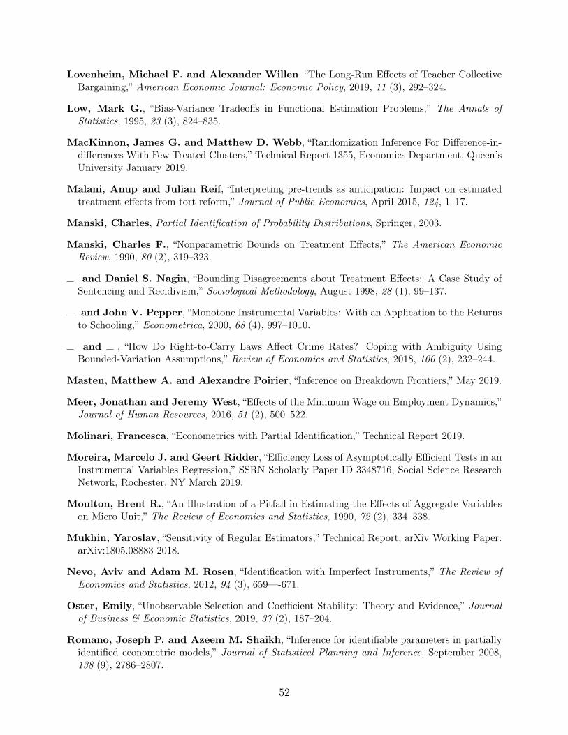
Lovenheim, Michael F. and Alexander Willen, “The Long-Run Effects of Teacher CollectiveBargaining,” American Economic Journal: Economic Policy, 2019, 11 (3), 292–324.

Low, Mark G., “Bias-Variance Tradeoffs in Functional Estimation Problems,” The Annals ofStatistics, 1995, 23 (3), 824–835.

MacKinnon, James G. and Matthew D. Webb, “Randomization Inference For Difference-in-differences With Few Treated Clusters,” Technical Report 1355, Economics Department, Queen’sUniversity January 2019.

Malani, Anup and Julian Reif, “Interpreting pre-trends as anticipation: Impact on estimatedtreatment effects from tort reform,” Journal of Public Economics, April 2015, 124, 1–17.

Manski, Charles, Partial Identification of Probability Distributions, Springer, 2003.

Manski, Charles F., “Nonparametric Bounds on Treatment Effects,” The American EconomicReview, 1990, 80 (2), 319–323.

and Daniel S. Nagin, “Bounding Disagreements about Treatment Effects: A Case Study ofSentencing and Recidivism,” Sociological Methodology, August 1998, 28 (1), 99–137.

and John V. Pepper, “Monotone Instrumental Variables: With an Application to the Returnsto Schooling,” Econometrica, 2000, 68 (4), 997–1010.

and , “How Do Right-to-Carry Laws Affect Crime Rates? Coping with Ambiguity UsingBounded-Variation Assumptions,” Review of Economics and Statistics, 2018, 100 (2), 232–244.

Masten, Matthew A. and Alexandre Poirier, “Inference on Breakdown Frontiers,” May 2019.

Meer, Jonathan and Jeremy West, “Effects of the Minimum Wage on Employment Dynamics,”Journal of Human Resources, 2016, 51 (2), 500–522.

Molinari, Francesca, “Econometrics with Partial Identification,” Technical Report 2019.

Moreira, Marcelo J. and Geert Ridder, “Efficiency Loss of Asymptotically Efficient Tests in anInstrumental Variables Regression,” SSRN Scholarly Paper ID 3348716, Social Science ResearchNetwork, Rochester, NY March 2019.

Moulton, Brent R., “An Illustration of a Pitfall in Estimating the Effects of Aggregate Variableson Micro Unit,” The Review of Economics and Statistics, 1990, 72 (2), 334–338.

Mukhin, Yaroslav, “Sensitivity of Regular Estimators,” Technical Report, arXiv Working Paper:arXiv:1805.08883 2018.

Nevo, Aviv and Adam M. Rosen, “Identification with Imperfect Instruments,” The Review ofEconomics and Statistics, 2012, 94 (3), 659—-671.

Oster, Emily, “Unobservable Selection and Coefficient Stability: Theory and Evidence,” Journalof Business & Economic Statistics, 2019, 37 (2), 187–204.

Romano, Joseph P. and Azeem M. Shaikh, “Inference for identifiable parameters in partiallyidentified econometric models,” Journal of Statistical Planning and Inference, September 2008,138 (9), 2786–2807.

52

, , and Michael Wolf, “A Practical Two-Step Method for Testing Moment Inequalities,”Econometrica, 2014, 82 (5), 1979–2002.

Rosenbaum, Paul, “Sensitivity Analysis in Observational Studies,” in B. S. Everitt and D. C.Howell, eds., Encyclopedia of Statistics in Behavioral Science, 2005.

and Donald Rubin, “Assessing Sensitivity to an Unobserved Binary Covariate in an Observa-tional Study with Binary Outcome,” Journal of the Royal Statistical Society. Series B, 1983, 45(2), 212–218.

Roth, Jonathan, “Pre-test with Caution: Event-study Estimates After Testing for ParallelTrends,” Working paper, 2019.

Sant’Anna, Pedro H. C. and Jun B. Zhao, “Doubly Robust Difference-in-Differences Estima-tors,” arXiv:1812.01723 [econ], September 2019. arXiv: 1812.01723.

Schrijver, Alexander, Theory of Linear and Integer Programming, Wiley-Interscience, 1986.

Sun, Yu and Karen X Yan, “Inference on Difference-in-Differences average treatment effects: Afixed-b approach,” Journal of Econometrics, 2019, 211 (2), 560–588.

Słoczyński, Tymon, “A General Weighted Average Representation of the Ordinary and Two-StageLeast Squares Estimands,” 2018.

Tamer, Elie, “Partial Identification in Econometrics,” Annual Review of Economics, 2010, 2, 167–195.

Wolfers, Justin, “Did Unilateral Divorce Laws Raise Divorce Rates? A Reconciliation and NewResults,” American Economic Review, 2006, 96, 1802–1820.

53