AN IDL CODE TO PLOT THE POTENTIAL FIELD SOURCE

SURFACE (PFSS) MODEL SYNOPTIC CHART

A.Cora, S.Mancuso

Rapporto nr. 131 14/04/2010

Table of ContentsABSTRACT...............................................................................................................................................3INTRODUCTION.....................................................................................................................................3POTENTIAL FIELD SOURCE SURFACE MODEL..............................................................................3METHOD OF COMPUTATION..............................................................................................................5THE IDL CODE........................................................................................................................................7CONCLUSION..........................................................................................................................................8REFERENCE.............................................................................................................................................9Appendix A : PFSS_model.pro..................................................................................................................9Appendix B : READ_G_H.pro..................................................................................................................9Appendix C : NL_function_list.pro.........................................................................................................10Appendix D : NL_main.pro.....................................................................................................................13

ABSTRACT

Various structures seen in the solar corona, such as coronal streamers, might be regarded as tracers of the magnetic field lines. Using photospheric data, the configuration of the coronal and heliospheric field can be calculated by means of the Potential Field Source Surface (PFSS) model. The model provides a 3D picture of the heliospheric magnetic field in a range of radial distances between 1 solar radius and the source surface. In this internal report, we briefly describe the PFSS model assumptions and the mathematical approach adopted in searching for its solutions. Applying this method (based on the expansion on spherical harmonics) we develop a simple IDL code to plot the PFSS synoptic charts.

INTRODUCTIONIt has been observed that the large-scale geometry of the coronal magnetic field plays an important role in the brightness distribution of the white light corona (Guhathakurta et al. 1996), but also of the intensity distributions of the UV corona (see Fig. 1). The oppositely directed magnetic fields of the northern and southern hemispheres and the flow of the fast solar wind from the north and south polar coronal holes divide the heliospheric plasma in two regions, with opposite polarity. These two regions are separated by a current sheet, which is a neutral surface of symmetry for propagation of heliospheric plasma. The PFSS model (Alschuler & Newkirk 1969; Schatten et al.1969) has been the first method that has allowed mapping the observed photospheric magnetic field into the corona. This model has been widely used for comparing the magnetic field with density structures in the corona and the interplanetary solar wind and in calculating the position of coronal holes and of the heliospheric current sheet. In fact, above the source surface the magnetic field lines are radial, and so the position of the neutral line at any distance from the Sun can be inferred by radial extrapolation of the source surface neutral line.

Fig.1: Carrington Rotation 1910 showing the Lyman α spectral line intensity observed by SOHO/UVCS at the East limb with the slit at a heliocentric distance of 2.6 Rsun superposed to the coronal magnetic field calculated from the photospheric field distributed by the Solar

Wilcox Observatory (WSO) at the URL: http://wso.stanford.edu/synsourcel.html.

POTENTIAL FIELD SOURCE SURFACE MODEL

The potential field source surface (PFSS) model is basically a method that allows to extrapolate the photospheric magnetic field through the corona into the heliosphere. In general, this model takes global radial Carrington synoptic maps as input. In these maps, photospheric fields are sampled on a heliographic coordinate, evenly spaced either in latitude or sine-latitude steps. The PFSS mode describes the magnetic field in the volume between the photosphere and the source surface, the latter typically located at a heliocentric distance of 2.5 Rsun. This

volume is assumed to be current-free, and the magnetic field is forced to be radial at the source surface to model the effect of the solar magnetic field frozen into the coronal plasma and then dragged out by the solar wind as it flows radially outward (see Fig. 2). This model has several advantages: it is simple to be developed and implemented, it requires relatively modest computer resources, and it can resolve global structures on spatial scales beyond those that can be handled by the observations. Because of its simplicity, however, the PFSS model makes some critical assumptions. In particular, by assuming that the electric currents in the corona are negligible, it implies that the global magnetic field can be considered approximately as potential. Studies of the coupling of the coronal field into the heliosphere do suggest that the global coronal magnetic field is often largely potential, although neglecting electric currents implies, for example, that the model cannot directly incorporate time-depending phenomena, such as magnetic reconnections or transient events, and cannot properly describe other small-scale non-potential coronal features. Another critical assumption is that the source surface is spherical, although its might be more consistent with one of a prolate spheroid along the rotation axis.

The PFSS model assumes that the coronal magnetic field is quasi-stationary and that it can be thus described analytically as a series expansion of spherical harmonics. Coronal currents are neglected so as to allow unique solutions in closed form. The Laplace's equation within an annular volume above the photosphere is thus solved in terms of a spherical harmonic expansion, the coefficients of which are derived from the Carrington maps of the photospheric magnetic field.

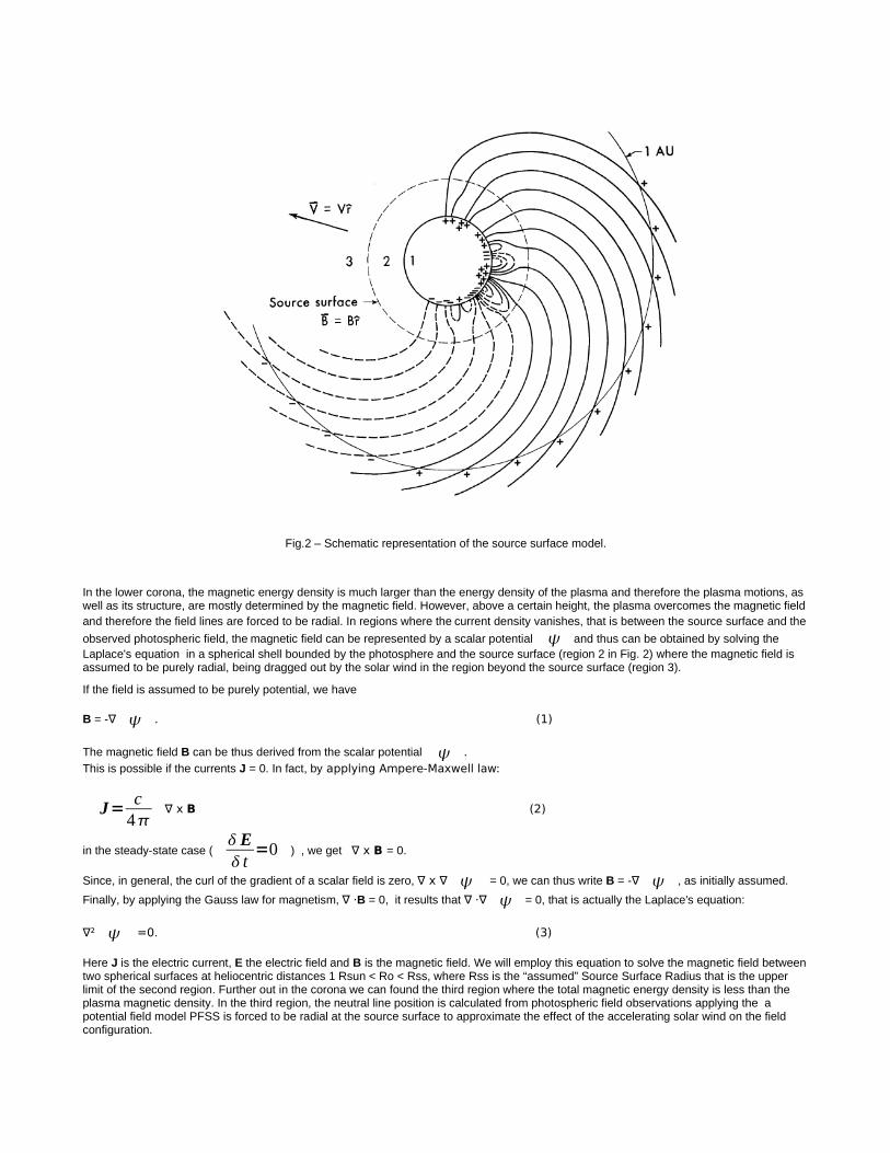
Fig.2 – Schematic representation of the source surface model.

In the lower corona, the magnetic energy density is much larger than the energy density of the plasma and therefore the plasma motions, as well as its structure, are mostly determined by the magnetic field. However, above a certain height, the plasma overcomes the magnetic field and therefore the field lines are forced to be radial. In regions where the current density vanishes, that is between the source surface and the

observed photospheric field, the magnetic field can be represented by a scalar potential and thus can be obtained by solving the Laplace's equation in a spherical shell bounded by the photosphere and the source surface (region 2 in Fig. 2) where the magnetic field is assumed to be purely radial, being dragged out by the solar wind in the region beyond the source surface (region 3).

If the field is assumed to be purely potential, we have

B = -∇ . (1)

The magnetic field B can be thus derived from the scalar potential . This is possible if the currents J = 0. In fact, by applying Ampere-Maxwell law:

J= c4

∇ x B (2)

in the steady-state case (E t

=0 ) , we get ∇ x B = 0.

Since, in general, the curl of the gradient of a scalar field is zero, ∇ x ∇ = 0, we can thus write B = -∇ , as initially assumed.

Finally, by applying the Gauss law for magnetism, ∇ ·B = 0, it results that ∇ ·∇ = 0, that is actually the Laplace's equation:

∇² =0. (3)

Here J is the electric current, E the electric field and B is the magnetic field. We will employ this equation to solve the magnetic field between two spherical surfaces at heliocentric distances 1 Rsun < Ro < Rss, where Rss is the “assumed” Source Surface Radius that is the upper limit of the second region. Further out in the corona we can found the third region where the total magnetic energy density is less than the plasma magnetic density. In the third region, the neutral line position is calculated from photospheric field observations applying the a potential field model PFSS is forced to be radial at the source surface to approximate the effect of the accelerating solar wind on the field configuration.

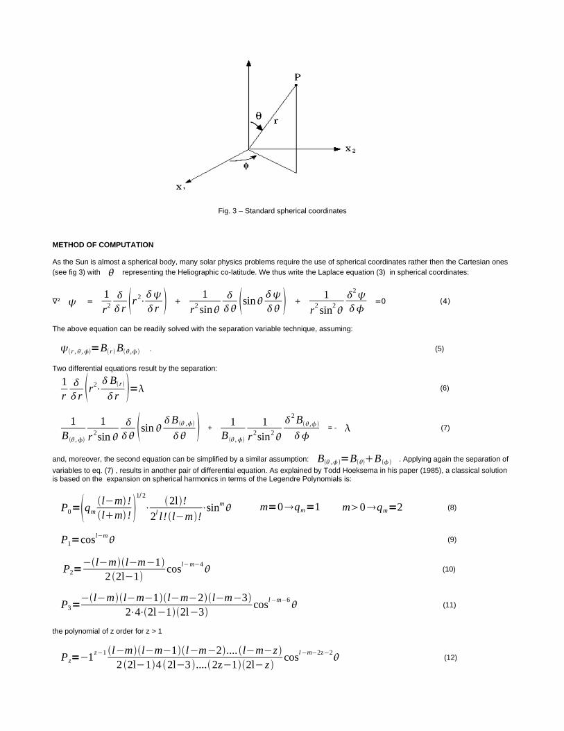
Fig. 3 – Standard spherical coordinates

METHOD OF COMPUTATION

As the Sun is almost a spherical body, many solar physics problems require the use of spherical coordinates rather then the Cartesian ones

(see fig 3) with representing the Heliographic co-latitude. We thus write the Laplace equation (3) in spherical coordinates:

∇² =1

r2

r r 2⋅

r +1

r2 sin sin

+1

r2 sin2

2

=0 (4)

The above equation can be readily solved with the separation variable technique, assuming:

r , ,=Br B , . (5)

Two differential equations result by the separation:

1r

r r2⋅

Br

r = (6)

1B ,

1

r 2sin

sin

B ,

+1

B ,

1r 2sin2

2B,

= - (7)

and, moreover, the second equation can be simplified by a similar assumption: B ,=BB . Applying again the separation of

variables to eq. (7) , results in another pair of differential equation. As explained by Todd Hoeksema in his paper (1985), a classical solution is based on the expansion on spherical harmonics in terms of the Legendre Polynomials is:

P0=qm l−m !lm ! 1/2

⋅2l!

2l l! l−m!⋅sinm m=0qm=1 m0qm=2 (8)

P1=cosl−m (9)

P2=−l−ml−m−1

2 2l−1cos

l−m−4 (10)

P3=−l−ml−m−1l−m−2l−m−3

2⋅4⋅2l−12l−3cosl−m−6

(11)

the polynomial of z order for z > 1

Pz=−1z−1 l−ml−m−1l−m−2.... l−m−z 2 2l−14 2l−3 ....2z−12l− z

cosl−m−2z−2 (12)

and finally the Legendre polynomial with Schatten normalization:

Plm =∑

z

Pz (13)

Using this form for the Legendre polynomials the three components of the magnetic field between the photosphere and the source surface can be written:

Br=∑l=1

N

∑m=0

l

P lmg lmcosmhlm sinm⋅{l1 Ror

l2

−l rRss l−1

cl} (14)

B=−∑l=1

N

∑m=0

l Plm

g lmcosmhlm sinm⋅{Ror

l2

cl rRss l−1

} (15)

B=∑l=1

N

∑m=0

l msin

P lmg lmcosm−hlm sinm⋅{ Ror

l2

cl rRss l−1

} (16)

where :

• Plm

are the Legendre polynomials with Schatten normalization

• g l ,m and h l ,m are the harmonic coefficient, obtained from the observed photospheric magnetic field by the Wilcox Solar Observatory and available at the URL: http://wso.stanford.edu

• R0 is the heliocentric distance of the sphere where we calculate the magnetic field components expressed in solar radii;

• Rss is the radius of the source surface expressed in solar radii;

• and cl=− R0

Rss l2

(17)

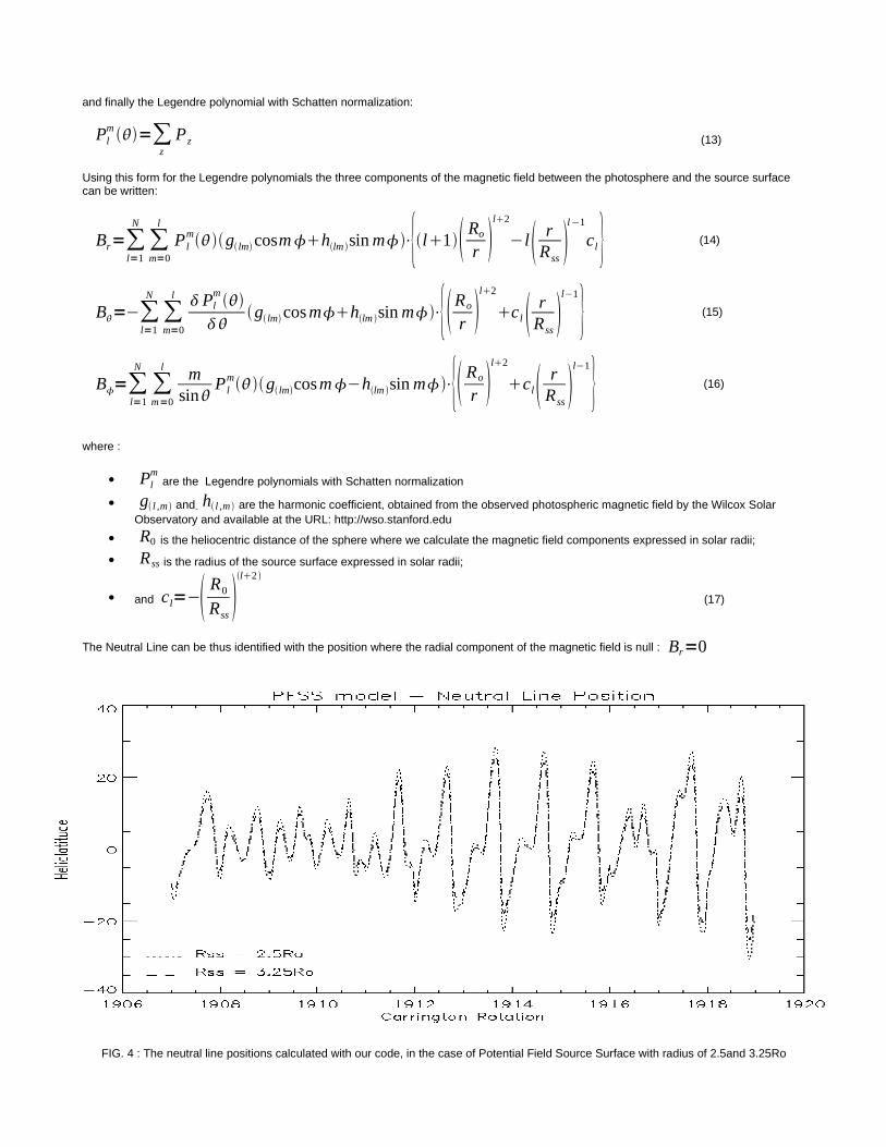
The Neutral Line can be thus identified with the position where the radial component of the magnetic field is null : Br=0

FIG. 4 : The neutral line positions calculated with our code, in the case of Potential Field Source Surface with radius of 2.5and 3.25Ro

THE IDL CODE

We are interested in studying the UV spectral lines intensity distribution with respect to the Neutral Line. We have thus developed a simple IDL code in order to obtain the Neutral Line position on a sphere at a heliocentric distance 2.5 Ro, assuming different Source Surface Radii (see fig.4). After running the IDL compiler environment, it is possible to initialize the package by typing:

@PFSS_model

This command compiles the following IDL procedures:APPROX, a procedure developed by S.Giordano to approximate a value to a fixed decimal digit.READ_G_H, the procedures developed to read the harmonic coefficient distribute by the Solar Wilcox Observatory. These coefficients will be stored in the array g and h ,which will be used by the main program.NL_function_list contains the Legendre polynomial functions with Schatten normalization as described in eq. (13), coefficient Cl as eq. (17) and the function deg2rad converts angles measured in degree units in radians.NL_main uses the functions written into NL, computes the magnetic field, and draws the plots

Fig.5 : We used Carrington Rotation 1910 Radial Component of Magnetic Field at a Source Surface Radius =2.5, calculated by WSO (up side) to verify the resulting of our code, as the Carrington Rotation 1910 Radial Component of Magnetic Field at Rss =2.5Ro

CONCLUSION

We are used to assume as a simple model of the heliospheric magnetic field an archimedian spiral field directed radially. The calculation of the neutral line position for different Carrington rotations offers us the possibility to represent in a realistic way this kind of model (see fig.7). Furthermore, as explained before, we are interested in calculating the Neutral Line Position (by studying the UV spectral line intensity distribution) and implement the code that does this operation.

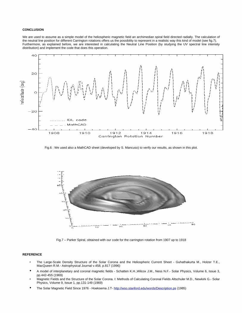
Fig.6 : We used also a MathCAD sheet (developed by S. Mancuso) to verify our results, as shown in this plot.

Fig.7 – Parker Spiral, obtained with our code for the carrington rotation from 1907 up to 1918

REFERENCE

• The Large-Scale Density Structure of the Solar Corona and the Heliospheric Current Sheet - Guhathakurta M., Holzer T.E., MacQueen R.M.- Astrophysical Journal v.458, p.817 (1996)

• A model of interplanetary and coronal magnetic fields - Schatten K.H.,Wilcox J.M., Ness N.F.- Solar Physics, Volume 6, Issue 3, pp.442-455 (1969)

• Magnetic Fields and the Structure of the Solar Corona. I: Methods of Calculating Coronal Fields Altschuler M.D., Newkirk G.- Solar Physics, Volume 9, Issue 1, pp.131-149 (1969)

• The Solar Magnetic Field Since 1976 - Hoeksema J.T- http://wso.stanford.edu/words/Description.ps (1985)

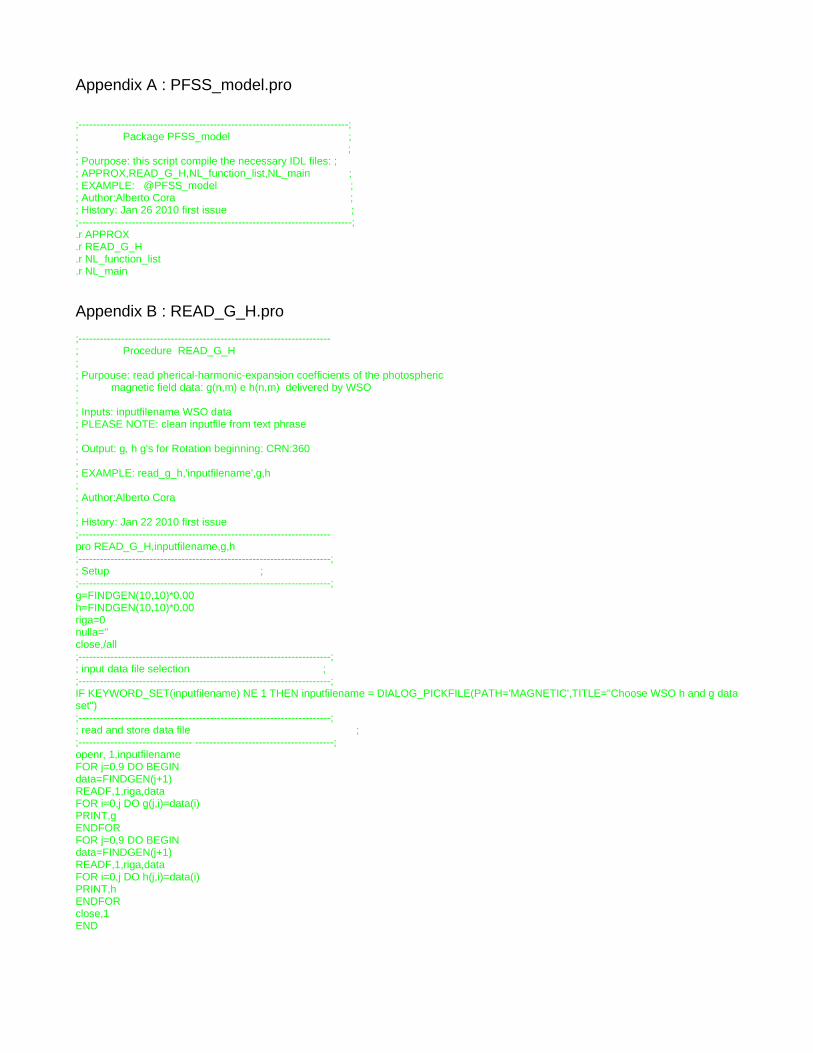
Appendix A : PFSS_model.pro

;----------------------------------------------------------------------------;; Package PFSS_model ;; ;; Pourpose: this script compile the necessary IDL files: ;; APPROX,READ_G_H,NL_function_list,NL_main ;; EXAMPLE: @PFSS_model ;; Author:Alberto Cora ;; History: Jan 26 2010 first issue ; ;-----------------------------------------------------------------------------;.r APPROX.r READ_G_H.r NL_function_list.r NL_main

Appendix B : READ_G_H.pro

;-----------------------------------------------------------------------; Procedure READ_G_H;; Purpouse: read pherical-harmonic-expansion coefficients of the photospheric ; magnetic field data: g(n,m) e h(n,m) delivered by WSO;; Inputs: inputfilename WSO data ; PLEASE NOTE: clean inputfile from text phrase; ; Output: g, h g's for Rotation beginning: CRN:360;; EXAMPLE: read_g_h,'inputfilename',g,h;; Author:Alberto Cora;; History: Jan 22 2010 first issue;-----------------------------------------------------------------------pro READ_G_H,inputfilename,g,h;-----------------------------------------------------------------------;; Setup ;;-----------------------------------------------------------------------;g=FINDGEN(10,10)*0.00h=FINDGEN(10,10)*0.00riga=0nulla=''close,/all;-----------------------------------------------------------------------;; input data file selection ;;-----------------------------------------------------------------------;IF KEYWORD_SET(inputfilename) NE 1 THEN inputfilename = DIALOG_PICKFILE(PATH='MAGNETIC',TITLE="Choose WSO h and g data set");-----------------------------------------------------------------------;; read and store data file ;;-------------------------------- ---------------------------------------;openr, 1,inputfilenameFOR j=0,9 DO BEGINdata=FINDGEN(j+1)READF,1,riga,dataFOR i=0,j DO g(j,i)=data(i)PRINT,gENDFORFOR j=0,9 DO BEGINdata=FINDGEN(j+1)READF,1,riga,dataFOR i=0,j DO h(j,i)=data(i)PRINT,hENDFORclose,1END

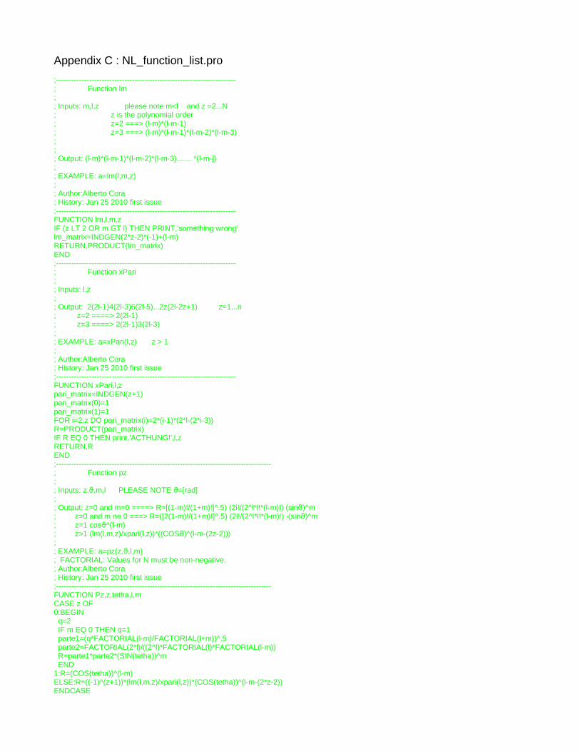
Appendix C : NL_function_list.pro

;-----------------------------------------------------------------------; Function lm ; ; Inputs: m,l,z please note m<l and z =2...N ; z is the polynomial order ; z=2 ===> (l-m)*(l-m-1) ; z=3 ===> (l-m)*(l-m-1)*(l-m-2)*(l-m-3) ; ; ; Output: (l-m)*(l-m-1)*(l-m-2)*(l-m-3)....... *(l-m-j) ; ; EXAMPLE: a=lm(l,m,z) ; ; Author:Alberto Cora ; History: Jan 25 2010 first issue ;-----------------------------------------------------------------------FUNCTION lm,l,m,zIF (z LT 2 OR m GT l) THEN PRINT,'something wrong'lm_matrix=INDGEN(2*z-2)*(-1)+(l-m)RETURN,PRODUCT(lm_matrix)END;-----------------------------------------------------------------------; Function xPari ; ; Inputs: l,z ; ; Output: 2(2l-1)4(2l-3)6(2l-5)...2z(2l-2z+1) z=1...n ; z=2 ====> 2(2l-1); z=3 ====> 2(2l-1)3(2l-3); ; EXAMPLE: a=xPari(l,z) z > 1 ; ; Author:Alberto Cora ; History: Jan 25 2010 first issue ;-----------------------------------------------------------------------FUNCTION xPari,l,zpari_matrix=INDGEN(z+1)pari_matrix(0)=1pari_matrix(1)=1FOR i=2,z DO pari_matrix(i)=2*(i-1)*(2*l-(2*i-3))R=PRODUCT(pari_matrix)IF R EQ 0 THEN print,'ACTHUNG!',l,zRETURN,REND;-------------------------------------------------------------------------------------; Function pz ; ; Inputs: z, ,m,l PLEASE NOTE =[rad] ϑ ϑ; ; Output: z=0 and m=0 ====> R=[(1-m)!/(1+m)!]^.5) (2i!/(2^l*l!*(l-m)!) (sin )^m ϑ; z=0 and m ne 0 ===> R=([2(1-m)!/(1+m)!]^.5) (2i!/(2^l*l!*(l-m)!) ∙(sin )^m ϑ; z=1 cos ^(l-m) ϑ; z>1 (lm(l,m,z)/xpari(l,z))*((COS )^(l-m-(2z-2))) ϑ; ; EXAMPLE: a=pz(z, ,l,m) ϑ; FACTORIAL: Values for N must be non-negative. ; Author:Alberto Cora ; History: Jan 25 2010 first issue ;-------------------------------------------------------------------------------------FUNCTION Pz,z,tetha,l,mCASE z OF0:BEGIN q=2 IF m EQ 0 THEN q=1 parte1=(q*FACTORIAL(l-m)/FACTORIAL(l+m))^.5 parte2=FACTORIAL(2*l)/((2^l)*FACTORIAL(l)*FACTORIAL(l-m)) R=parte1*parte2*(SIN(tetha))^m END1:R=(COS(tetha))^(l-m)ELSE:R=((-1)^(z+1))*(lm(l,m,z)/xpari(l,z))*(COS(tetha))^(l-m-(2*z-2))ENDCASE

RETURN,REND;-------------------------------------------------------------------------------------; Function dpz ; ; Inputs: z, ,m,l PLEASE NOTE =[rad] ϑ ϑ; ; Author:Alberto Cora ; History: Feb 18 2010 first issue ;-------------------------------------------------------------------------------------FUNCTION dPz,z,tetha,l,mCASE z OF0:BEGIN q=2 IF m EQ 0 THEN q=1 parte1=(q*FACTORIAL(l-m)/FACTORIAL(l+m))^.5 parte2=FACTORIAL(2*l)/((2^l)*FACTORIAL(l)*FACTORIAL(l-m)) R=parte1*parte2*m*((SIN(tetha))^(m-1))*COS(tetha) END1:R=-(l-m)*((COS(tetha))^(l-m-1))*SIN(tetha)ELSE:R=(-(-1)^(z+1))*(lm(l,m,z)/xpari(l,z))*(l-m-(2*z-2))*((COS(tetha))^(l-m-(2*z-2)-1))*SIN(tetha)ENDCASERETURN,REND;-----------------------------------------------------------------------; Function p (Legendre polynomial ) ; ; Inputs: ,l,m,N PLEASE NOTE m<l =[rad] ϑ ϑ; ; Output: ; ; EXAMPLE: a=p( ,l,m) ϑ; ; Author:Alberto Cora ; History: Jan 26 2010 first issue ;-----------------------------------------------------------------------FUNCTION P,tetha,l,m,Npararray=DBLARR(N+1)*0FOR j=0,N-1 DO pararray(j)=Pz(j+1,tetha,l,m)R=Pz(0,tetha,l,m)*TOTAL(pararray)RETURN,REND;-----------------------------------------------------------------------; Function dp (Derivate Legendre polynomial) ; ;FUNCTION dP,tetha,l,m,Npararray=DBLARR(N+1)*0FOR j=0,N-1 DO pararray(j)=dPz(j+1,tetha,l,m)R=dPz(0,tetha,l,m)*TOTAL(pararray)RETURN,REND;-----------------------------------------------------------------------; Function deg2rad ; ; Inputs: ,m,l PLEASE NOTE =[deg] ϑ ϑ; ; Output: =[rad] ϑ; ; EXAMPLE: a=deg2rad( ) ϑ; ; Author:Alberto Cora ; History: Jan 26 2010 first issue ;-----------------------------------------------------------------------FUNCTION deg2rad,degRETURN,!pi*(deg/180d0)END;-----------------------------------------------------------------------; Function c ; Inputs: l,Ro,Rss Ro photosphere radius ; Rss source surface radius ; ; Output: -(Ro/Rss)^(l+2) ;

; EXAMPLE: c(l,Ro,Rss) ; ; ; Author:Alberto Cora ; History: Jan 27 2010 first issue ;-----------------------------------------------------------------------FUNCTION c,l,Ro,RssRETURN,-(Ro/Rss)^(l+2)END;-----------------------------------------------------------------------; Function Br ; ; Inputs: r, ,φ,Ro,Rss,g,h PLEASE NOTE: g, h array ϑ; =[deg] ϑ; ; Output: Br radial component Magnetic Field ; ; EXAMPLE: a=Br( ) ϑ; ; Author:Alberto Cora ; History: Jan 26 2010 first issue ;-----------------------------------------------------------------------FUNCTION Br,radius,tetha,phi,g,h,Ro,Rss,NsecondSUM=DBLARR(N+1) FOR l=1,N DO BEGIN ; l=1...N firstSUM=DBLARR(l+1)*0 FOR m=0,l DO BEGIN part1=g(l,m)*COS(DOUBLE(m*phi))+h(l,m)*SIN(DOUBLE(m*phi)) part2=DOUBLE((l+1)*((Ro/radius)^(l+2))-l*c(l,Ro,Rss)*((radius/Rss)^(l-1))) firstSUM(m)=P(tetha,l,m,N)*part1*part2 ENDFOR secondSUM(l)=TOTAL(firstSUM)ENDFORR=TOTAL(secondSUM)RETURN,REND;-----------------------------------------------------------------------; Function Bt ; ; Inputs: r, ,φ,Ro,Rss,g,h PLEASE NOTE: g, h array ϑ; =[deg] ϑ; ; Output: Bt tetha component Magnetic Field ; ; EXAMPLE: a=Bt(r, ,φ,Ro,Rss,g,h) ϑ; ; Author:Alberto Cora ; History: Feb 18 2010 first issue ;-----------------------------------------------------------------------FUNCTION Bt,radius,tetha,phi,g,h,Ro,Rss,NsecondSUM=DBLARR(N+1) ;this empty array will contain the 2nd summatoryFOR l=1,N DO BEGIN ; l=1...N see mathcad script firstSUM=DBLARR(l+1)*0 FOR m=0,l DO BEGIN part1=g(l,m)*COS(DOUBLE(m*phi))+h(l,m)*SIN(DOUBLE(m*phi)) part2=DOUBLE(((Ro/radius)^(l+2))+c(l,Ro,Rss)*((radius/Rss)^(l-1))) firstSUM(m)=part1*part2*dP(tetha,l,m,N) ENDFOR secondSUM(l)=TOTAL(firstSUM)ENDFORR=-TOTAL(secondSUM)RETURN,REND;-----------------------------------------------------------------------; Function Bf ; ; Inputs: r, ,φ,Ro,Rss,g,h PLEASE NOTE: g, h array ϑ; =[deg] ϑ; ; Output: Bf phi component Magnetic Field ; ; EXAMPLE: a=Bf( ) ϑ;

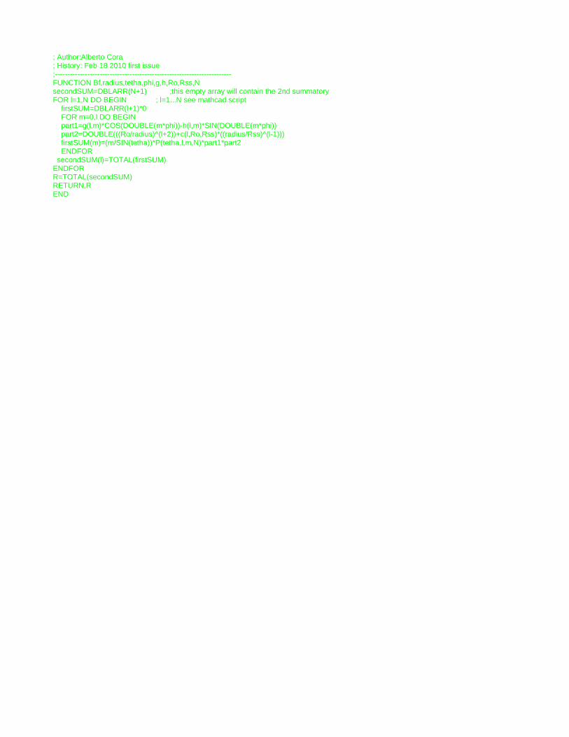
; Author:Alberto Cora ; History: Feb 18 2010 first issue ;-----------------------------------------------------------------------FUNCTION Bf,radius,tetha,phi,g,h,Ro,Rss,NsecondSUM=DBLARR(N+1) ;this empty array will contain the 2nd summatoryFOR l=1,N DO BEGIN ; l=1...N see mathcad script firstSUM=DBLARR(l+1)*0 FOR m=0,l DO BEGIN part1=g(l,m)*COS(DOUBLE(m*phi))-h(l,m)*SIN(DOUBLE(m*phi)) part2=DOUBLE(((Ro/radius)^(l+2))+c(l,Ro,Rss)*((radius/Rss)^(l-1))) firstSUM(m)=(m/SIN(tetha))*P(tetha,l,m,N)*part1*part2 ENDFOR secondSUM(l)=TOTAL(firstSUM)ENDFORR=TOTAL(secondSUM)RETURN,REND

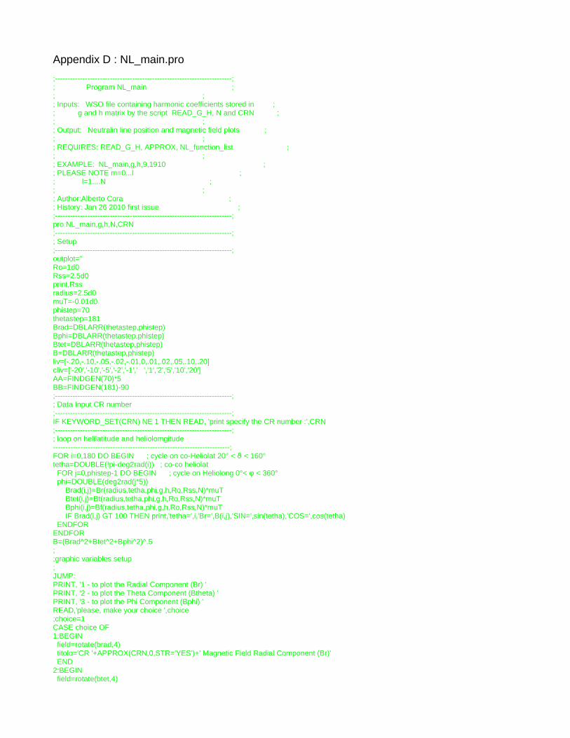
Appendix D : NL_main.pro

;-----------------------------------------------------------------------;; Program NL_main ;; ;; Inputs: WSO file containing harmonic coefficients stored in ; ; g and h matrix by the script READ_G_H, N and CRN ;; ;; Output: Neutralin line position and magnetic field plots ;; ;; REQUIRES: READ_G_H, APPROX, NL_function_list ;; ;; EXAMPLE: NL_main,g,h,9,1910 ; ; PLEASE NOTE m=0...l ;; l=1....N ;; ;; Author:Alberto Cora ;; History: Jan 26 2010 first issue ; ;-----------------------------------------------------------------------;pro NL_main,g,h,N,CRN;-----------------------------------------------------------------------;; Setup;-----------------------------------------------------------------------;outplot=''Ro=1d0Rss=2.5d0print,Rssradius=2.5d0muT=-0.01d0phistep=70thetastep=181Brad=DBLARR(thetastep,phistep)Bphi=DBLARR(thetastep,phistep)Btet=DBLARR(thetastep,phistep)B=DBLARR(thetastep,phistep)liv=[-.20,-.10,-.05,-.02,-.01,0,.01,.02,.05,.10,.20]cliv=['-20','-10','-5','-2','-1',' ','1','2','5','10','20']AA=FINDGEN(70)*5BB=FINDGEN(181)-90;-----------------------------------------------------------------------;; Data Input CR number;-----------------------------------------------------------------------;IF KEYWORD_SET(CRN) NE 1 THEN READ, 'print specify the CR number :',CRN;-----------------------------------------------------------------------;; loop on helilatitude and heliolomgitude-----------------------------------------------------------------------; FOR i=0,180 DO BEGIN ; cycle on co-Heliolat 20° < < 160°ϑtetha=DOUBLE(!pi-deg2rad(i)) ; co-co heliolat FOR j=0,phistep-1 DO BEGIN ; cycle on Heliolong 0°< φ < 360° phi=DOUBLE(deg2rad(j*5)) Brad(i,j)=Br(radius,tetha,phi,g,h,Ro,Rss,N)*muT Btet(i,j)=Bt(radius,tetha,phi,g,h,Ro,Rss,N)*muT Bphi(i,j)=Bf(radius,tetha,phi,g,h,Ro,Rss,N)*muT IF Brad(i,j) GT 100 THEN print,'tetha=',i,'Br=',B(i,j),'SIN=',sin(tetha),'COS=',cos(tetha) ENDFORENDFORB=(Brad^2+Btet^2+Bphi^2)^.5;;graphic variables setup;JUMP:PRINT, '1 - to plot the Radial Component (Br) 'PRINT, '2 - to plot the Theta Component (Btheta) 'PRINT, '3 - to plot the Phi Component (Bphi) 'READ,'please, make your choice ',choice;choice=1CASE choice OF1:BEGIN field=rotate(brad,4) titolo='CR '+APPROX(CRN,0,STR='YES')+' Magnetic Field Radial Component (Br)' END2:BEGIN field=rotate(btet,4)

titolo='CR '+APPROX(CRN,0,STR='YES')+' Magnetic Field Theta Component (Btheta)' END3:BEGIN field=rotate(bphi,4) titolo='CR '+APPROX(CRN,0,STR='YES')+' Magnetic Field Phi Component (Bphi)' ENDELSE: BEGIN PRINT, '??????' GOTO, JUMPENDENDCASEWINDOW,1,Xsize=720,ysize=400contour,field,AA,BB,level=liv,xrange=[0,360],XSTYLE=1,yrange=[-90,90],ystyle=1,C_ANNOTATION = cliv,TITLE=titolo,Xtitle='Heliolongitude (deg)',Ytitle='Heliolatitude (deg)'contour,field,AA,BB,level=0,thic=2,C_ANNOTATION ='0',/OVERPLOToplot,[0,360],[0,0],line=2SET_PLOT,'PS'

contour,field,AA,BB,level=liv,xrange=[0,360],XSTYLE=1,yrange=[-90,90],ystyle=1,C_ANNOTATION = cliv,TITLE=titolo,Xtitle='Heliolongitude (deg)',Ytitle='Heliolatitude (deg)'contour,field,AA,BB,level=0,thic=2,C_ANNOTATION ='0',/OVERPLOToplot,[0,360],[0,0],line=2close, /allprint, 'plot stored into the file idl.ps'SET_PLOT,'X' ;; Calculate CRN.phase;; Neutra Line Data Store subroutine; NL data are store in two variables:; XNEUTRALINE DOUBLE = Array[889] format CRN,phase; YNEUTRALINE DOUBLE = Array[889] Heliolat + nord - sud; the session are saved as NL[CRN].savXNEUTRALINE=DBLARR(phistep)YNEUTRALINE=DBLARR(phistep)

FOR j=0,phistep-1 DO XNEUTRALINE(j)=DOUBLE(CRN+(j*5d0/360d0))YLINE=DBLARR(thetastep)FOR i=0,thetastep-1 DO YLINE(i)=DOUBLE(i)-90d0

FOR j=0,phistep-1 DO BEGIN WINDOW,2,Xsize=720,ysize=400 PLOT,YLINE,Brad(*,j),psym=0 T=DBLARR(thetastep*10) FOR i=0,(thetastep*10)-1 DO T(i)=DOUBLE((i/10d0)-90d0) ZZ = SPLINE(YLINE,Brad(*,j),T) OPLOT,T,ZZ FOR i=0,(thetastep*10)-2 DO IF (ZZ(i)*ZZ(i+1)) LT 0 THEN YNEUTRALINE(j)=DOUBLE((T(i)+T(i+1))/2)

OPLOT,[YNEUTRALINE(j),YNEUTRALINE(j)],[0,0],PSYM=4 wait,.3 plot, XNEUTRALINE(*),YNEUTRALINE(*) ENDFOR

save,filename='NL'+APPROX(CRN,0,STR='YES')+'.sav',XNEUTRALINE,YNEUTRALINE

END