an image-based approach to three-dimensional …
TRANSCRIPT

AN IMAGE-BASED APPROACHTO THREE-DIMENSIONAL
COMPUTER GRAPHICS
by
Leonard McMillan Jr.
A dissertation submitted to the faculty of the University of North Carolina at Chapel Hill inpartial fulfillment of the requirements for the degree of Doctor of Philosophy in theDepartment of Computer Science.
Chapel Hill
1997
Approved by:
______________________________Advisor: Gary Bishop
______________________________Reader: Anselmo Lastra
______________________________Reader: Stephen Pizer

ii
© 1997Leonard McMillan Jr.
ALL RIGHTS RESERVED

iii
ABSTRACT
Leonard McMillan Jr.
An Image-Based Approach to Three-Dimensional Computer Graphics
(Under the direction of Gary Bishop)
The conventional approach to three-dimensional computer graphics produces images
from geometric scene descriptions by simulating the interaction of light with matter. My
research explores an alternative approach that replaces the geometric scene description with
perspective images and replaces the simulation process with data interpolation.
I derive an image-warping equation that maps the visible points in a reference image to
their correct positions in any desired view. This mapping from reference image to desired
image is determined by the center-of-projection and pinhole-camera model of the two images
and by a generalized disparity value associated with each point in the reference image. This
generalized disparity value, which represents the structure of the scene, can be determined from
point correspondences between multiple reference images.
The image-warping equation alone is insufficient to synthesize desired images because
multiple reference-image points may map to a single point. I derive a new visibility algorithm
that determines a drawing order for the image warp. This algorithm results in correct visibility
for the desired image independent of the reference image’s contents.
The utility of the image-based approach can be enhanced with a more general pinhole-
camera model. I provide several generalizations of the warping equation’s pinhole-camera
model and discuss how to build an image-based representation when information about the
reference image’s center-of-projection and camera model is unavailable.
iv
ACKNOWLEDGMENTS
I owe tremendous debts of gratitude to the following:
• My advisor and long time friend Gary Bishop who first challenged me to return to
graduate school and has subsequently served as both teacher and advocate during the
entire process.
• My committee members, Fred Brooks, James Coggins, Henry Fuchs, Anselmo Lastra,
Steve Pizer, and Turner Whitted who have been endless sources of wisdom,
enthusiasm, and inspiration.
• The department research faculty, in particular Vern Chi for his advice on limiting
cases; and John Poulton, Nick England, and Mary Whitton for their enthusiasm and
support.
• My department colleagues and fellow students, in particular Bill Mark for his
collaborations and willingness to endure my ramblings.
• My parents Leonard McMillan Sr. and Joan McMillan for nurturing, encouragement,
and their willingness to allow me to take things apart, while knowing that I might not
succeed in putting them back together. Also, my brother John McMillan whose
belongings I so often dismantled.
I wish both to thank and to dedicate this dissertation to my wife Donna for all of the love that
she brings to my life, and to my daughter Cassie for all of the joy that she brings.

v

vi
TABLE OF CONTENTS
CHAPTER 1 INTRODUCTION.......................................................................................................... 1
1.1 CONVENTIONAL COMPUTER GRAPHICS MODELS ........................................................................... 3
1.2 THESIS STATEMENT AND CONTRIBUTIONS ...................................................................................... 4
1.3 MOTIVATION.................................................................................................................................. 6
1.4 PREVIOUS WORK ............................................................................................................................ 7
1.4.1 Images as approximations ........................................................................................................ 8
1.4.2 Images as databases................................................................................................................ 11
1.4.3 Images as models ......................................................................................................... .......... 14
1.5 DISCUSSION.................................................................................................................................. 17
CHAPTER 2 THE PLENOPTIC MODEL......................................................................................... 19
2.1 THE PLENOPTIC FUNCTION........................................................................................................... 20
2.2 GEOMETRIC STRUCTURES IN PLENOPTIC SPACE ............................................................................ 23
2.3 ALTERNATIVE MODELS ................................................................................................................ 26
2.4 SAMPLING AN ENVIRONMENT ...................................................................................................... 26
2.5 SUMMARY .................................................................................................................................... 28
CHAPTER 3 A WARPING EQUATION.......................................................................................... 30
3.1 FROM IMAGES TO RAYS................................................................................................................. 31
3.2 A GENERAL PLANAR-PINHOLE MODEL ....................................................................................... 31
3.3 A WARPING EQUATION FOR SYNTHESIZING PROJECTIONS OF A SCENE......................................... 33
3.4 RELATION TO PREVIOUS RESULTS ................................................................................................. 41
3.5 RESOLVING VISIBILITY................................................................................................................... 44
3.5.1 Visibility Algorithm .............................................................................................................. 45
3.6 RECONSTRUCTION ISSUES ............................................................................................................. 49
3.7 OCCLUSION AND EXPOSURE ERRORS ............................................................................................ 55
3.8 SUMMARY .................................................................................................................................... 59

vii
CHAPTER 4 OTHER PINHOLE CAMERAS .................................................................................. 61
4.1 ALTERNATIVE PLANAR PINHOLE-CAMERA MODELS .................................................................... 61
4.1.1 Application-specific planar pinhole-camera models ................................................................ 62
4.1.2 A canonical pinhole model ..................................................................................................... 66
4.1.3 Planar calibration .................................................................................................................. 67
4.2 NONLINEAR PINHOLE-CAMERA MODELS..................................................................................... 68
4.3 PANORAMIC PINHOLE CAMERAS.................................................................................................. 68
4.3.1 Cylindrical pinhole-camera model .......................................................................................... 70
4.3.2 Spherical model...................................................................................................................... 76
4.4 DISTORTED PINHOLE-CAMERA MODELS....................................................................................... 77
4.4.1 Fisheye pinhole-camera model ................................................................................................ 80
4.4.2 Radial distortion pinhole-camera model ................................................................................. 82
4.5 MODIFYING WARPING EQUATIONS .............................................................................................. 85
4.6 REAL CAMERAS............................................................................................................................. 86
4.6.1 Nonlinear camera calibration................................................................................................. 86
4.7 SUMMARY .................................................................................................................................... 87
CHAPTER 5 WARPING WITHOUT CALIBRATION................................................................... 88
5.1 EPIPOLAR GEOMETRIES AND THE FUNDAMENTAL MATRIX........................................................... 88
5.1.1 The Fundamental Matrix....................................................................................................... 90
5.1.2 Determining a Fundamental Matrix from Point Correspondences ......................................... 93
5.2 RELATING THE FUNDAMENTAL MATRIX TO THE IMAGE-WARPING EQUATION ............................. 95
5.2.1 Image Warps Compatible with a Fundamental Matrix........................................................... 98
5.3 PHYSICAL CONSTRAINTS ON PROJECTIVE MAPS...........................................................................102
5.3.1 Same-Camera Transformations.............................................................................................102
5.3.2 Determining a Camera Model from a Same-Camera Transformation ....................................105
5.3.3 Closed-form solutions for the intrinsic camera-parameters ....................................................108
5.4 DERIVING A PLANAR PINHOLE-CAMERA MODEL FROM IMAGES..................................................111
5.4.1 Scalar matrix quantities of transforms with known epipolar geometries ................................112
5.4.2 Finding a Camera Solution ...................................................................................................114
5.5 AN EXAMPLE...............................................................................................................................119
5.6 DISCUSSION.................................................................................................................................122
CHAPTER 6 COMPUTING VISIBILITY WITHOUT DEPTH ....................................................124
6.1 DEFINITIONS................................................................................................................................124

viii
6.2 PROOF .........................................................................................................................................126
6.3 MAPPING TO A PLANAR VIEWING SURFACE ................................................................................130
6.4 DISCUSSION.................................................................................................................................135
CHAPTER 7 COMPARING IMAGE-BASED AND GEOMETRIC METHODS.......................137
7.1 THE IMAGE-BASED GRAPHICS PIPELINE.......................................................................................138
7.2 AN INVERSE-MAPPED APPROACH TO IMAGE-BASED RENDERING ...............................................141
7.3 DISCUSSION.................................................................................................................................146
CHAPTER 8 CONCLUSIONS AND FUTURE WORK... ERROR! BOOKMARK NOT DEFINED.
8.1 SYNOPSIS .....................................................................................................................................147
8.1.1 Advantages of image-based computer graphics ......................................................................147
8.1.2 Disadvantages of image-based computer graphics .................................................................149
8.1.3 Limitations of image-based methods......................................................................................150
8.2 FUTURE WORK .............................................................................................................................151
8.2.1 Sampling an environment.....................................................................................................151
8.2.2 Reconstruction and resampling.............................................................................................152
8.2.3 Incorporating information from multiple reference images ....................................................152
8.2.4 Image-based computer graphics systems................................................................................153
8.2.5 View dependence...................................................................................................................153
8.2.6 Plenoptic approximation methods other than warping ..........................................................154
D.1 OVERVIEW..................................................................................................................................165
D.2 MODULES AND CLASSES.............................................................................................................166
D.3 SOURCE ......................................................................................................................................166
D.3.1 Vwarp.java ..........................................................................................................................166
D.3.2 Reference.java ......................................................................................................................170
D.3.3 PlanarReference.java............................................................................................................170
D.3.4 Vector3D.java .....................................................................................................................176
D.3.5 Raster.java...........................................................................................................................180

ix
LIST OF FIGURES
Figure 1-1: Traditional approach to three-dimensional computer graphics..................................... 1
Figure 1-2: Traditional approach to computer vision......................................................................... 2
Figure 1-3: Conventional partitioning of computer vision and computer graphics ...................... 17
Figure 2-1: Parameters of the plenoptic function.............................................................................. 21
Figure 2-2: A bundle of rays ............................................................................................................... 23
Figure 2-3: A plane and convex region specified by three points ................................................... 24
Figure 2-4: A plane and planar subspace specified by two viewing points and a ray................... 24
Figure 2-5: A plane specified by a viewing point and a great circle ............................................... 25
Figure 2-6: A correspondence............................................................................................................. 25
Figure 2-7: The parameterization of rays used in both light-fields and lumigraphs ..................... 26
Figure 3-1: Mapping image-space point to rays................................................................................ 32
Figure 3-2: Relationship of the image-space basis vectors to the ray origin................................... 33
Figure 3-3: A point in three-dimensional space as seen from two pinhole cameras...................... 34
Figure 3-4: The depth-from-stereo camera configuration ................................................................ 35
Figure 3-5: Vector diagram of planar warping equation.................................................................. 37
Figure 3-6: A third view of the point �X ............................................................................................ 38
Figure 3-7: Reprojection of an image with the same center-of-projection ...................................... 41
Figure 3-8: A planar region seen from multiple viewpoints ............................................................ 42
Figure 3-9: A desired center-of-projection projected onto the reference image ............................. 46
Figure 3-10: Figure of nine regions..................................................................................................... 46
Figure 3-11: A desired center-of-projection that divides the reference image into 4 sheets ......... 47
Figure 3-12: A desired center-of-projection that divides the reference image into 2 sheets ......... 47
Figure 3-13: A desired center-of-projection that divides the reference image into 1 sheet ........... 48
Figure 3-14: Enumeration direction ................................................................................................... 48
Figure 3-15: A Gaussian cloud representation of image-space points ............................................ 51
Figure 3-16: Example image warps using different reconstruction methods................................. 55

x
Figure 3-17: Exposures at occluding boundaries .............................................................................. 56
Figure 3-18: Exposure error on a smooth surface boundary ........................................................... 57
Figure 3-19: Occlusion errors introduced by polynomial reconstruction....................................... 58
Figure 3-20: An external exposure error............................................................................................ 59
Figure 4-1: Illustration of a simple pinhole-camera model .............................................................. 62
Figure 4-2: Illustration of the frustum model.................................................................................... 64
Figure 4-3: Illustration of computer-vision model............................................................................ 65
Figure 4-4: The canonical cylindrical pinhole-camera viewing surface .......................................... 70
Figure 4-5: A cylindrical pinhole model of an operating room scene ............................................. 72
Figure 4-6: A cylindrical pinhole model of Sitterson Hall................................................................ 72
Figure 4-7: A wide-angle cylindrical pinhole model of the old well ............................................... 72
Figure 4-8: A cylindrical projection.................................................................................................... 75
Figure 4-9: Desired images from a cylinder-to-plane warp ............................................................. 75
Figure 4-10: The viewing surface of the canonical spherical pinhole-camera model..................... 76
Figure 4-11: Wide-angle distortion from a 100° field-of-view planar projection ........................... 78
Figure 4-12: A cylindrical projection with a 100° field-of-view....................................................... 79
Figure 4-13: A fisheye projection with a 100° field-of-view............................................................. 80
Figure 4-14: A fisheye (left) and planar (right) projection of a yard scene ..................................... 81
Figure 4-15: View surface of a fisheye pinhole model ...................................................................... 82
Figure 4-16: Two images exhibiting radial distortion....................................................................... 83
Figure 4-17: Mapping onto cubic radial distortion surfaces ............................................................ 84
Figure 5-1: An epipolar geometry ...................................................................................................... 89
Figure 5-2: A camera shown with rays converging towards a vanishing point............................. 90
Figure 5-3: Mapping of a unit sphere before and after a skew-symmetric matrix......................... 97
Figure 5-4: The projective transformations compatible with a given fundamental matrix..........101
Figure 5-5: The skew and aspect ratio properties of a planar-pinhole camera..............................107
Figure 5-6: Surface of potentially compatible projective transformations .....................................115
Figure 5-7: The solution space of compatible same-camera transformations................................117
Figure 5-8: ...........................................................................................................................................120
Figure 5-9 ............................................................................................................................................120
Figure 5-10...........................................................................................................................................121
Figure 5-11...........................................................................................................................................121
Figure 6-1: Spherical coordinate frames embedded in a Cartesian coordinate system................125
Figure 6-2: An epipolar plane defined by a ray and two centers-of-projection ............................126

xi
Figure 6-3: A multiplicity induced by translation of coordinate frames........................................127
Figure 6-4: A multiplicity illustrated in an epipolar plane..............................................................128
Figure 6-5: A reprojection order that guarantees an occlusion-compatible result ........................130
Figure 6-6: Occlusion-compatible traversals mapped onto planar viewing surfaces ...................131
Figure 6-7: Occlusion-compatible planar traversal orders..............................................................131
Figure 6-8: Spherical enumeration directions projected onto a plane............................................132
Figure 6-9: Subdivision of the image plane into four sheets ...........................................................132
Figure 6-10: An equivalent enumeration along the rows and columns of a planar image...........133
Figure 6-11: A mapping of epipolar planes onto a cylindrical viewing surface............................136
Figure 7-1: Standard geometry-based graphics pipeline.................................................................138
Figure 7-2: A image-based graphics pipeline ...................................................................................140
Figure 7-3: Algorithm for a display-driven rendering approach ...................................................142
Figure 7-4: Projection of a desired ray onto a reference image.......................................................142
Figure 7-5: Endpoints of a ray in a reference image ........................................................................144
Figure 7-6: Display-driven image-based rendering.........................................................................146

xii
LIST OF EQUATIONS
Equation 2-1: Plenoptic Function ....................................................................................................... 21
Equation 3-1: Planar mapping function............................................................................................. 32
Equation 3-2: Specification of a 3D point in terms of pinhole-camera parameters........................ 34
Equation 3-3: Transformation of a ray in one camera to its corresponding ray in another .......... 35
Equation 3-4: Simplified planar ray-to-ray mapping ....................................................................... 35
Equation 3-5: Simplified planar mapping equation.......................................................................... 36
Equation 3-6: Normalized planar mapping equation....................................................................... 36
Equation 3-7: Aligned image-space mapping ................................................................................... 36
Equation 3-8: Difference between image coordinates for stereo camera configuration ................ 36
Equation 3-9: Stereo disparity ............................................................................................................ 37
Equation 3-10: Planar image-warping equation................................................................................ 38
Equation 3-11: 4 × 3 matrix formulation of warping equation ........................................................ 40
Equation 3-12: Warping equation as rational expressions ............................................................... 40
Equation 3-13: Image reprojection ..................................................................................................... 41
Equation 3-14: Equation of a plane ............................................................................................. ....... 42
Equation 3-15: Mapping of a common plane seen at two centers-of-projection ............................ 43
Equation 3-16: Projection of the reference image plane in the desired image................................ 44
Equation 3-17: Locus of three-space points along a ray ................................................................... 44
Equation 3-18: Projection of desired center-of-projection onto reference image ........................... 45
Equation 3-19: Jacobian of the warping equation ............................................................................. 52
Equation 3-20: Jacobian determinant of the warping equation ....................................................... 52
Equation 3-21: Camera-model matrix, H, and the structure matrix, G .......................................... 53
Equation 3-22: Radius of differential region ..................................................................................... 53
Equation 3-23: Differential change induced by mapping................................................................. 53
Equation 3-24: Projection of differential circular disk...................................................................... 54
Equation 3-25: Expanded expression for differential circular disk ................................................. 54

xiii
Equation 3-26: Screen-space extent for projected circular disk ....................................................... 54
Equation 4-1: A simple pinhole-camera model................................................................................. 62
Equation 4-2: Finding an ideal camera’s field-of-view from its focal length.................................. 63
Equation 4-3: Frustum model of a pinhole camera........................................................................... 63
Equation 4-4: Computer-vision pinhole-camera model ................................................................... 64
Equation 4-5: Deriving a canonical-pinhole camera from a general one ........................................ 66
Equation 4-6: A normalization of the canonical pinhole-camera model......................................... 67
Equation 4-7: Canonical cylindrical mapping function.................................................................... 70
Equation 4-8: Prewarp to remove skew parameter from a cylindrical mapping function............ 71
Equation 4-9: Inverse of the cylindrical mapping function.............................................................. 71
Equation 4-10: Cylinder-to-cylinder correspondence....................................................................... 72
Equation 4-11: Special cylinder-to-cylinder warping equation ....................................................... 72
Equation 4-12: General cylinder-to-cylinder warping equation...................................................... 73
Equation 4-13: Aligned cylinder-to-cylinder warping equation...................................................... 73
Equation 4-14: Aligned cylinder-to-cylinder warping equation without skew.............................. 73
Equation 4-15: Cylinder-to-cylinder reprojection ............................................................................. 74
Equation 4-16: The plane defined by a line through two points and a center-of-projectionError! Bookmark not def
Equation 4-17: Mapping of line onto a cylindrical viewing surface................................................ 72
Equation 4-18: Cylinder-to-plane warping equation........................................................................ 73
Equation 4-19: Expanded cylinder-to-plane warping equation....................................................... 73
Equation 4-20: Spherical mapping function ...................................................................................... 74
Equation 4-21: Prewarp to remove spherical skew .......................................................................... 75
Equation 4-22: Inverse spherical pinhole-camera model ................................................................. 76
Equation 4-23: Fisheye distortion mapping function ....................................................................... 80
Equation 4-24: Inverse fisheye distortion mapping function........................................................... 81
Equation 4-25: Cubic distortion mapping function .......................................................................... 82
Equation 4-26: Inverse cubic distortion mapping function.............................................................. 83
Equation 4-27: General geometrically consistent warp .................................................................... 84
Equation 5-1: The equation of a line in image space ........................................................................ 89
Equation 5-2: A correlation mapping points to lines....................................................................... 90
Equation 5-3: Fundamental matrix mapping a point to a line......................................................... 90
Equation 5-4: Reversing the fundamental matrix mapping............................................................. 91
Equation 5-5: Parameterization for a general fundamental matrix ................................................. 91
Equation 5-6: Linear equation in the coefficients of a fundamental matrix.................................... 92
xiv
Equation 5-7: Linear homogeneous system....................................................................................... 92
Equation 5-8: Singular-value decomposition of an approximate fundamental matrix ................. 93
Equation 5-9: Coordinate of the epipole in the second image ......................................................... 95
Equation 5-10: Fundamental matrix in terms of the planar-warping equation.............................. 96
Equation 5-11: Homogeneous system to find the second image’s epipole..................................... 97
Equation 5-12 ....................................................................................................................................... 98
Equation 5-13: Homogeneous coordinate of an epipole .................................................................. 98
Equation 5-14: Fundamental matrix in terms of an epipole and a projective transform............... 98
Equation 5-15: Equations for the elements of the fundamental matrix .......................................... 98
Equation 5-16: Projective transform’s elements in terms of the fundamental matrix ................... 99
Equation 5-17: Family of projective transformations compatible with a fundamental matrix ..... 99
Equation 5-18: Family of projective maps in terms of epipoles......................................................100
Equation 5-19: Same-camera transformation ...................................................................................101
Equation 5-20: Characteristic polynomial and eigenvalues of a rotation matrix ..........................101
Equation 5-21: Characteristic polynomial of scaled same-camera warp .......................................102
Equation 5-22: Scale factor that makes the determinant of σC equal one .....................................102
Equation 5-23: Constraints on a same-camera transformation.......................................................103
Equation 5-24: Rotational invariants of a same-camera transformation........................................104
Equation 5-25: Rotational invariants expressed as a matrix product.............................................104
Equation 5-26: Homogenous linear system determined by C ........................................................105
Equation 5-27: Planar-pinhole camera model of a same-camera transform..................................106
Equation 5-28: Constrained rotational-invariant matrix .................................................................107
Equation 5-29: Closed-form solution for the quantity b b⋅ in the general case............................108
Equation 5-30: Closed-form solution for the quantity c c⋅ in the general case.............................108
Equation 5-31: Closed-form solution for the quantities a c⋅ and b c⋅ in the general case..........108
Equation 5-32: The rotation between the camera models of a same-camera transform...............110
Equation 5-33: Planar warps resulting from the same camera .......................................................110
Equation 5-34: Determinant of a transform compatible with a given fundamental matrix .........111
Equation 5-35: Trace of a transform compatible with a given fundamental matrix .....................112
Equation 5-36: Vector of minor coefficients .....................................................................................112
Equation 5-37: Sum of the diagonal minors of compatible transforms..........................................112
Equation 5-38: Unit-determinant constraint.....................................................................................113
Equation 5-39: Trace-equals-sum-of-minors constraint ..................................................................113

xv
Equation 5-40: The trace of the desired transform prior to scaling................................................114
Equation 5-41: Expressions for h31, h32, and h33 in terms of σ and τ .................................................114
Equation 5-42: Three relational constraints on a same-camera transformation ............................115
Equation 5-43: Same-camera transform and adjoint compatible with F........................................115
Equation 5-44: Fundamental matrix used in Figure 5-8 ..................................................................117
Equation 5-45: Error function used in the global optimization ......................................................117
Equation 5-46: Estimated camera model ..........................................................................................118
Equation 5-47: Simple pinhole-camera model using manufacturer’s specs ..................................118
Equation 7-1: Using a 4 × 4 matrix multiplier to compute the image warp ..................................138
Equation 7-2: Image-based view port clipping ................................................................................138
Equation 7-3: Maximum extent of epipolar line segment ...............................................................141
Equation 7-4: Minimum extent of epipolar line segment................................................................142
Equation 7-5: A parametric form of a line........................................................................................143
Equation 7-6: The tau form of a line ........................................................................................... ......143
Equation 7-7: Disparity required to map a reference point to a desired point .............................144
Equation 7-8: Theta value at a point on the ray’s extent .................................................................144
Equation 7-9: Minimum disparity required for a given tau value .................................................144

1
&KDSWHU �
INTRODUCTION
“Computer graphics concerns the pictorial synthesis of real or imaginary objects fromtheir computer-based models, whereas the related field of image processing treats theconverse process: the analysis of scenes, or the reconstruction of models of 2D or 3Dobjects from their pictures.”
Foley, van Dam, Feiner, and Hughes
The field of three-dimensional computer graphics has long focused on the problem of
synthesizing images from geometric models. These geometric models, in combination with
surface descriptions characterizing the reflective properties of each geometric element, represent
a desired scene that is to be rendered by the computer graphics system. Computationally, the
computer-graphics image synthesis process is a simulation problem in which light’s interactions
with the supplied scene description are computed.
Figure 1-1: Traditional approach to three-dimensional computer graphics
Conventional computer vision considers the opposite problem of synthesizing geometric
models from images. In addition to images, computer-vision systems depend on accurate
camera models and estimates of a camera’s position and orientation in order to synthesize the
desired geometric models. Often a simple reflectance model of the observed scene’s surfaces is
another integral part of a computer-vision system. The image-processing methods employed in

2
computer vision include the identification of image features and filtering to remove noise and to
resample the source images at desired scales. In addition to image processing, geometric
computations are required to map the identified image features to their positions in a three-
dimensional space.
Figure 1-2: Traditional approach to computer vision
The efforts of computer graphics and computer vision are generally perceived as
complementary because the results of one field can frequently serve as an input to the other.
Computer graphics often looks to the field of computer vision for the generation of complex
geometric models, whereas computer vision relies on computer graphics both for the generation
of reference images and for viewing results. Three-dimensional geometry has been the
fundamental interface between the fields of computer vision and computer graphics since their
inception. Seldom has the appropriateness of this link been challenged.
The research presented in this dissertation suggests an alternative interface between the
image analysis of computer vision and the image synthesis of computer graphics. In this work I
describe methods for synthesizing images, comparable to those produced by conventional three-
dimensional computer graphics methods, directly from other images without a three-
dimensional geometric representation. I will demonstrate that the computations used in this
image-based approach are fundamentally different from the simulation techniques used by
traditional three-dimensional computer graphics.
In this chapter, I first discuss the various model representations commonly used in
computer graphics today, and how all of these modeling approaches stem from a common
geometric heritage. Then I will propose an image-based alternative to three-dimensional
graphics, and discuss why one is needed. I will finally consider previous research in which
images have served as computer graphics models.

3
1.1 Conventional Computer Graphics Models
Since its inception, a primary goal of computer graphics has been the synthesis of
images from models. It is standard for images to be represented as two-dimensional arrays of
pixels stored in the frame buffer of the computer. Model descriptions, however, are much more
varied.
One modeling technique represents the boundaries between objects as a series of two-
dimensional surfaces embedded within a three-dimensional space. This approach is called a
boundary representation. Boundary representations can be further broken down according to the
degree of the surface description. A first-degree description might consist entirely of polygonal
facets specified by the coordinates of their vertices. A higher-degree description might describe
a curved surface patch whose three-dimensional shape is defined in terms of a series of three-
dimensional control points.
Another representation commonly used to describe three-dimensional models is the
Boolean combinations of solids. In this method the primitive descriptions enclose a volume,
rather than specify a surface. There are two popular variants of this approach: constructive
solid geometry (CSG) and binary spatial partitioning (BSP). In constructive solid geometry the
desired shape is specified in terms of a tree of elementary solids that are combined using simple
set operations. The BSP approach is a special case of CSG in which the only modeling primitive
used is a region of space, called a half-space, that is bounded on one side by a plane. The only
operation allowed in a BSP model’s tree representation is the intersection of the child node’s
half-space with the space enclosed by its parent.
Enumerated space representations are a third popular modeling description. The
distinguishing attribute of enumerated space models is that they represent objects as a set of
discrete volume elements. An example is volumetric modeling in which the spatial
relationships between elements are encoded implicitly within a three-dimensional data
structure.
A common attribute of all these popular modeling paradigms is that they describe shape
in three spatial dimensions. In addition, an orthogonal set of axes and a unit of measure are
usually assumed. Models of this type, regardless of whether they represent surface boundaries,
solids, or discrete volumes, describe entities from a three-dimensional Euclidean geometry.

4
Using Euclidean geometry as a basis for describing models has many practical
advantages. Euclidean geometry is the geometry of our everyday experience. Our common
notions of length, area, and volume are all deeply rooted within a Euclidean description.
Unfortunately, the extraction of Euclidean information from two-dimensional images is known
to be a difficult problem [Kanatani89]. This is because Euclidean geometry is an unnatural
choice for describing the relationships between images and image points. A better choice is
projective geometry. The value of Euclidean geometric models for image synthesis has been
established. But, the question still remains—how might images be synthesized based on
projective relationships?
1.2 Thesis Statement and Contributions
This research presents an alternative modeling paradigm in which the underlying
representation is a set of two-dimensional images rather than a collection of three-dimensional
geometric primitives. The resulting visualization process involves a systematic projective
mapping of the points from one image to their correct position in another image. Correctness
will be defined as being consistent with the equivalent projections of a static three-dimensional
Euclidean geometry. In short, I propose to generate valid views of a three-dimensional scene by
synthesizing images from images without an explicit Euclidean representation.
The central thesis of this research is that
Three-dimensional computer graphics can be synthesized using only images andinformation derivable from them. The resulting computation process is a signalreconstruction problem rather than a simulation as in traditional three-dimensionalcomputer graphics.
Three central problems must be addressed in order to synthesize three-dimensional
computer graphics from images. The first problem is the determination of mapping functions
that move the points of a source image to new positions in a desired image. This mapping is
constrained to be consistent with reprojections of the three-dimensional scene depicted in the
source. In Chapter 3 I derive this family of warping functions. The second problem of image-
based computer graphics is the accurate determination of the subset of source points that are
visible from other viewpoints in the absence of a geometric description. Chapter 3 presents an
algorithm for computing such a visibility solution for the case of planar projections. This result
is expanded and generalized to other viewing surfaces in Chapter 6. The third issue that must
be resolved in order to build viable image-based computer graphics systems is the

5
reconstruction of continuous models from sampled image representations. Discretely sampled
images are a common form of data representation that are amenable to computation, and the
classical approaches to two-dimensional image reconstruction are not directly extensible to the
nonlinear behaviors induced by projection and changes in visibility. In Chapter 3, I will address
many of the issues of this reconstruction and make the argument that, in the absence of
additional information, the problem is essentially ambiguous. I then propose two alternative
approaches to the reconstruction problem based on two extreme assumptions about the three-
dimensional space depicted by a scene.
This dissertation contributes to the field of computer science a family of algorithms useful for
rendering image-based computer graphics. Included among these are
• an image-warping equation for transforming the points of one image totheir appropriate position in another image as seen from a differentviewing point
• a visibility algorithm that determines which points from one image canbe seen from another viewing point without any knowledge of theshapes represented in the original image
• a method for approximating the continuous shapes of the visible figuresin an image when given only a sampled image representation
Furthermore, this research establishes new links between the synthesis techniques of computer
graphics and the analysis methods of computer vision. This work also compares and contrasts
the image-based and geometry-based approaches to computer graphics.
I will provide substantial evidence supporting the following assertions:
• three-dimensional computer graphics can be synthesized using onlyimages and information derivable from them
• image-based computer graphics is a signal reconstruction problemrather than a simulation problem like traditional computer graphics
• given known viewing parameters, an image-to-image mapping functioncan be established that is consistent with arbitrary projections of a staticthree-dimensional Euclidean geometry from the same view
• even with unknown viewing parameters, under a reasonable set ofconstraints, an image-to-image mapping function can be established thatis consistent with arbitrary projections of a static three-dimensionalEuclidean geometry from the same view

6
• the visibility ordering of a reprojected-perspective image can beestablished without explicit knowledge of the geometry represented inthe original projection
• images synthesized using image-based methods can be generated usingfewer operations than geometry-based methods applied to anequivalent Euclidean representation
• the images synthesized from image-based methods are at least asrealistic as those images synthesized from geometric models usingsimulation methods
• the model acquisition process in image-based rendering is at least aseasy as extracting Euclidean geometric information from images
Having provided this short overview of the problem addressed by my research, I will
now explain why a solution to this problem is important.
1.3 Motivation
While geometry-based rendering technology has made significant strides towards
achieving photorealism, the process of creating accurate models is still nearly as difficult as it
was twenty-five years ago. Technological advances in three-dimensional scanning methods
provide some promise for simplifying the process of model building. However, these
automated model acquisition methods also verify our worst suspicions—the geometry of the
real-world is exceedingly complex.
Ironically, one of the primary subjective measures of image quality used in geometry-
based computer graphics is the degree to which a rendered image is indistinguishable from a
photograph. Consider, though, the advantages of using photographs (images) as the underlying
scene representation. Photographs, unlike geometric models, are both plentiful and easily
acquired, and needless to say, photorealistic. Images are capable of representing both the
geometric complexity and photometric realism of a scene in a way that is currently beyond our
modeling capabilities.
Throughout the three-dimensional computer graphics community, researchers, users,
and hardware developers alike, have realized the significant advantages of incorporating
images, in the form of texture maps, into traditional three-dimensional models. Texture maps
are commonly used to add fine photometric details as well as to substitute for small-scale
geometric variations. Texture mapping can rightfully be viewed as the precursor to image-

7
based computer graphics methods. In fact, the image-based approach discussed in this thesis
can be viewed as an extension of texture-mapping algorithms commonly used today. However,
unlike a purely image-based approach, an underlying three-dimensional model still plays a
crucial role with traditional texture maps.
In order to define an image-based computer graphics method, we need a principled
process for transforming a finite set of known images, which I will henceforth refer to as
reference images, into new images as they would be seen from arbitrary viewpoints. I will call
these synthesized images, desired images.
Techniques for deriving new images based on a series of reference images or drawings
are not new. A skilled architect, artist, draftsman, or illustrator can, with relative ease, generate
accurate new renderings of an object based on surprisingly few reference images. These
reference images are, frequently, illustrations made from certain cardinal views, but it is not
uncommon for them to be actual photographs of the desired scene taken from a different point-
of-view. One goal of this research is to emulate the finely honed skills of these artisans by using
computational powers.
While image-based computer graphics has come many centuries after the discovery of
perspective illustration techniques by artists, its history is still nearly as long as that of
geometry-based computer graphics. Progress in the field of image-based computer graphics can
be traced through at least three different scientific disciplines. In photogrammetry the problems
of distortion correction, image registration, and photometrics have progressed toward the
synthesis of desired images through the composition of reference images. Likewise, in computer
vision, problems such as navigation, discrimination, and image understanding have naturally led
in the same direction. In computer graphics, as discussed previously, the progression toward
image-based rendering systems was initially motivated by the desire to increase the visual
realism of the approximate geometric descriptions. Most recently, methods have been
introduced in which the images alone constitute the overall scene description. The remainder of
this introduction discusses previous works in image-based computer graphics and their
relationship to this work.
1.4 Previous Work
In recent years, images have supplemented the image generation process in several
different capacities. Images have been used to represent approximations of the geometric

8
contents of a scene. Collections of images have been employed as databases from which views
of a desired environment are queried. And, most recently, images have been employed as full-
fledged scene models from which desired views are synthesized. In this section, I will give an
overview of the previous work in image-based computer graphics partitioned along these three
lines.
1.4.1 Images as approximations
Images, mapped onto simplified geometry, are often used as an approximate
representation of visual environments. Texture mapping is perhaps the most obvious example
of this use. Another more subtle approximation involves the assumption that all, or most, of the
geometric content of a scene is located so far away from the viewer that its actual shape is
inconsequential.
Much of the pioneering work in texture mapping is attributable to the classic work of
Catmull, Blinn, and Newell. The flexibility of image textures as three-dimensional computer
graphics primitives has since been extended to include small perturbations in surface orientation
(bump maps) [Blinn76] and approximations to global illumination (environment and shadow
mapping) [Blinn76] [Greene86] [Segal92]. Recent developments in texture mapping have
concentrated on the use of visually rich textures mapped onto very approximate geometric
descriptions [Shade96] [Aliaga96][Schaufler96].
Texture mapping techniques rely on mapping functions to specify the relationship of the
texture’s image-space coordinates to their corresponding position on a three-dimensional model.
A comprehensive discussion of these mapping techniques was undertaken in [Heckbert86]. In
practice the specification of this mapping is both difficult and time consuming, and often
requires considerable human intervention. As a result, the most commonly used mapping
methods are restricted to very simple geometric descriptions, such as polygonal facets, spheres
and cylinders.
During the rendering process, these texture-to-model mapping functions undergo
another mapping associated with the perspective-projection process. This second mapping is
from the three-dimensional space of the scene’s representation to the coordinate space of the
desired image. In actual rendering systems, one or both of these mapping processes occurs in
the opposite or inverse order. For instance, when ray tracing, the mapping of the desired
image’s coordinates to the three-dimensional coordinates in the space of the visible object occurs

9
first. Then, the mapping from the three-dimensional object’s coordinates to the texture’s image-
space coordinates is found. Likewise, in z-buffering based methods, the mapping from the
image-space coordinate to texture’s image-space occurs during the rasterization process. These
inverse methods are known to be subject to aliasing and reconstruction artifacts. Many
techniques, including mip-maps [Williams83] and summed-area tables [Crow84] [Glassner86],
have been suggested to address these problems with texture mapping.
Another fundamental limitation of texture maps is that they rely solely on the geometry
of the underlying three-dimensional model to specify the object’s shape1. The precise
representation of three-dimensional shape using primitives suitable for the traditional approach
to computer graphics is, in itself, a difficult problem which has long been an active topic in
computer graphics research. When the difficulties of representing three-dimensional shape are
combined with the issues of associating a texture coordinate to each point on the surface (not to
mention the difficulties of acquiring suitable textures in the first place), the problem becomes
even more difficult.
It is conceivable that, given a series of photographs, a three-dimensional computer
model could be assembled. And, from those same photographs, various figures might be
identified, cropped, and the perspective distortions removed so that a texture might be
extracted. Then, using traditional three-dimensional computer graphics methods, renderings of
any desired image could be computed. While the process outlined is credible, it is both tedious
and prone to errors. The image-based approach to computer graphics described in this thesis
attempts to sidestep many of these intermediate steps by defining mapping functions from the
image-space of one or more reference images directly to the image-space of a desired image.
A new class of scene approximation results when an image is mapped onto the specific
geometric figure of the set of points at infinity. The mapping is accomplished in exactly the
same way that texture maps are applied to spheres, since each point on a sphere can be directly
associated with another point located an infinite distance from the sphere’s center. This
observation is also the basis of the environment maps mentioned previously. Environments
maps were, however, designed to be observed indirectly as either reflections within other
objects or as representations of a scene’s illumination environment. When such an image
1 Displacement maps [Upstill90] and, to a lesser extent, bump maps are exceptions to this
limitation.

10
mapping is intended for direct viewing, a new type of scene representation results. This is
characteristic of the work by Regan and Pose and the QuickTimeVR system.
Regan and Pose [Regan94] have described a hybrid system in which panoramic reference
images are generated using traditional geometry-based rendering systems at available rendering
rates, and interactive rendering is provided by the image-based subsystem. Their work
demonstrates some of the practical advantages of image-based computer graphics over
traditional geometric approaches. Among these are higher performance and reduced latency.
In Regan and Pose’s system, at any instant a user interacts with just a single reference image.
Their approach allows the user to make unconstrained changes in orientation about a fixed
viewing point, using a technique called address recalculation. Regan and Pose also discuss a
strategy for rendering nearby scene elements and integrating these results with the address
recalculation results. This approximation amounts to treating most scene elements as being
placed at infinity.
The image recalculation process of Regan and Pose is a special case of my image-based
rendering method, called reprojection. Reprojection, like address recalculation, allows for the
generation of arbitrary desired views where all of the points in the scene are considered to be an
infinite distance from the observer. This restriction results in a loss of both kinetic and
stereoscopic depth effects. However, with a very small modification, the same reprojection
method can be extended to allow objects to appear any distance from the viewer. In [Mark97]
the image-based methods described here have been applied to a hybrid rendering system
similar to the one described by Regan and Pose. Mark’s system demonstrates significant
advantages over address recalculation, and, by employing more than one reference image, he
shows how the need for rendering nearby scene elements can be eliminated.
A commercially available image-based computer graphics system, called QuickTimeVR
[Chen95], has been developed by Apple Computer Incorporated. In QuickTimeVR, the
underlying scene is represented by a set of cylindrical images. The system is able to synthesize
new planar views in response to a user’s input by warping one of these cylindrical images. This
is accomplished at highly interactive rates (greater than 20 frames per second) and is done
entirely in software. The system adapts both the resolution and reconstruction filter quality
based on the rate of the interaction. QuickTimeVR must be credited with exposing to a wide
audience the vast potential of image-based computer graphics. In particular, because of its

11
ability to use a series of stitched photographs as a reference image, it has enabled many new
computer graphics applications.
The QuickTimeVR system is also a reprojection method much like the address-
recalculation method described by Regan and Pose. Therefore, it is only capable of describing
image variations due to changes in viewing orientation. Translations of the viewing position
can only be approximated by selecting the cylindrical image whose center-of-projection is closest
to the current viewing position.
The panoramic representation afforded by the cylindrical image description provides
many practical advantages. It provides for the immersion of the user within the visual
environment, and it eliminates the need to consider the viewing angle when determining which
reference image is closest to a desired view. However, several normal photographs are required
to create a single cylindrical projection. These images must be properly registered and then
reprojected to construct the cylindrical reference image.
QuickTimeVR’s image-based approach has significant similarity to the approach
described here. Its rendering process is a special case of the cylinder-to-plane warping equation
(described in Chapter 4) in the case where all image points are computed as if they were an
infinite distance from the observer. However, the more general warping equation presented in
this thesis allows for the proper reprojection of points at any depth.
1.4.2 Images as databases
The movie-map system by Lippman [Lippman80] was one of the earliest attempts at
constructing a purely image-based computer graphics system. In a movie-map, many
thousands of reference images were stored on interactive video laser disks. These images could
be accessed randomly, according to the current viewpoint of the user. The system could also
accommodate simple panning, tilting, or zooming about these fixed viewing positions. The
movie-map approach to image-based computer graphics can also be interpreted as a table-based
approach, where the rendering process is replaced by a database query into a vast set of
reference images. This database-like structure is common to many image-based computer
graphics systems.
Movie-maps were unable to reconstruct all possible desired views. Even with the vast
storage capacities currently available on media such as laser disks, and the rapid development

12
of even higher capacity storage media, the space of all possible desired images appears so large
that any purely database-oriented approach will continue to be impractical in the near future.
Also, the very subtle differences between images observed from nearby points under similar
viewing conditions brings into question the overall efficiency of this approach. The image-based
rendering approach described in this thesis could be viewed as a reasonable compression
method for movie maps.
Levoy and Hanrahan [Levoy96] have described another database approach to computer
graphics in which the underlying modeling primitives are rays rather than images. The key
innovation of this technique, called light-field rendering, is the recognition that all of the rays that
pass through a slab of empty space which is enclosed between two planes can be described
using only four parameters (a two-dimensional coordinate on each plane) rather than the five
dimensions required for the typical specifications of a ray (a three-dimensional coordinate for
the ray’s origin and two angles to specify its direction.) This assumes that all of the rays will
enter the slab at one plane and exit through the other. They also describe an efficient technique
for generating the ray parameters needed to construct any arbitrary view.
The subset of rays originating from a single point on a light field’s entrance plane can be
considered as an image corresponding to what would have been seen at that point. Thus, the
entire two-parameter family of ray subsets originating from points on the entrance plane can be
considered as a set of reference images.
During the rendering process, the three-dimensional entrance and exit planes are
projected onto the desired viewing plane. The final image is constructed by determining the
image-space coordinates of the two points visible at a specified pixel coordinate (one coordinate
from the projected image of the entrance plane, and the second from the image of the exiting
plane). The desired ray can be looked up in the light field’s database of rays using these four
parameter values.
Image generation using light fields is inherently a database query process, much like the
movie map image-based process. The storage requirements for a light-field’s database of rays
can be very large. Levoy and Hanrahan discuss a lossy method for compressing light fields that
attempts to minimize some of the redundancy in the light-field representation.

13
The lumigraph [Gortler96] is another ray-database query algorithm closely related to the
light-field. It also uses a four-dimensional parameterization of the rays passing through a pair
of planes with fixed orientations. The primary differences in the two algorithms are the
acquisition methods used and the final reconstruction process. The lumigraph, unlike the light
field, considers the geometry of the underlying models when reconstructing desired views. This
geometric information is derived from image segmentations based on the silhouettes of image
features. The preparation of the ray database represented in a lumigraph requires considerable
preprocessing when compared to the light field. This is a result of the arbitrary camera poses
that are used to construct the database of visible rays. In a light-field, though, the reference
images are acquired by scanning a camera along a plane using a motion platform.
The lumigraph reconstruction process involves projecting each of the reference images
as they would have appeared when mapped onto the exit plane. The exit plane is then viewed
through an aperture on the entrance plane surrounding the center-of-projection of the reference
image. When both the image of the aperture on the entrance plane and the reference image on
the exit plane are projected as they would be seen from the desired view, the region of the
reference image visible through the aperture can be drawn into the desired image. The process
is repeated for each reference image. The lumigraph’s approach to image-based three-
dimensional graphics uses geometric information to control the blending of the image fragments
visible through these apertures.
Like the light-field, the lumigraph is a data intensive rendering process. The image-
based approach to computer graphics discussed in this research attempts to reconstruct desired
views based on far less information. First, the reference image nearest the desired view is used
to compute as much of the desired view as possible. Regions of the desired image that cannot
be reconstructed based on the original reference image are subsequently filled in from other
reference images.
The image-based approach proposed in this thesis can also be considered as a
compression method for both light fields and lumigraphs. Redundancy of the database
representation is reduced by considering the projective constraints induced by small variations
in the viewing configuration. Thus, an image point, along with its associated mapping function,
can be used to represent rays in many different images from which the same point is visible.

14
1.4.3 Images as models
Computer graphics methods have been developed where images serve as the
underlying representation. These methods handle the geometric relationships between image
points very differently. In the case of image morphing, the appearance of a dynamic Euclidean
geometry is often a desired effect. Another method, known as view interpolation relies on an
approximation to a true projective treatment in order to compute the mapping from reference
images to desired images. Also, additional Euclidean geometric information is required to
determine correct visibility. A third method, proposed by Laveau and Faugeras, is based on an
entirely projective approach to image synthesis and, therefore, is closely related to my work.
However, they have chosen to make a far more restrictive set of assumptions in their model,
which allows for an ambiguous Euclidean interpretation.
Image morphing is a popular image-based computer graphics technique [Beier92],
[Sietz96], [Wolberg90]. Generally, morphing describes a series of images representing a
transition between two reference images. These reference images can be considered as
endpoints along some path through time and/or space. An interpolation process is used to
reconstruct intermediate images along the path’s trajectory. Image morphing techniques have
been used to approximate dynamic changes in camera pose [Sietz96], dynamic changes in scene
geometry [Wolberg90], and combinations of these effects. In addition to reference images, the
morphing process requires that some number of points in each reference be associated with
corresponding points in the other. This association of points between images is called a
correspondence. This extra information is usually hand crafted by an animator. Most image-
morphing techniques make the assumption that the transition between these corresponding
points occurs at a constant rate along the entire path, thus amounting to a linear approximation.
Also, a graduated blending function is often used to combine the reference images after they are
mapped from their initial configuration to the desired point on the path. This blending function
is usually some linear combination of the two images based on what percentage of the path's
length has been traversed. The flexibility of image-morphing methods, combined with the
fluidity and realism of the image transitions generated, have made a dramatic impact on the
field of computer graphics, especially when considering how recently they have been
developed.
A subset of image morphing, called view morphing, is a special case of image-based
computer graphics. In view morphing the scene geometry is fixed, and the pose of the desired
views lies on a locus connecting the centers-of-projection of the reference images. With the

15
notable exception of the work done by Seitz, general image morphing makes no attempt to
constrain the trajectory of this locus, the characteristics of the viewing configurations, or the
shapes of the objects represented in the reference images. In this thesis, I will propose image
mapping functions which will allow desired images to be specified from any viewing point,
including those off the locus. Furthermore, these mapping functions, like those of Sietz, are
subject to constraints that are consistent with prescribed viewing conditions and the static
Euclidean shape of the objects represented in the reference images.
Chen and Williams [Chen93] have presented a view interpolation method for three-
dimensional computer graphics. It uses several reference images along with image
correspondence information to reconstruct desired views. Dense correspondence2 between the
pixels in reference images is established by a geometry-based rendering preprocess. During the
reconstruction process, linear interpolation between corresponding points is used to map the
reference images to the desired viewpoints, as in image morphing. In general, this interpolation
scheme gives a reasonable approximation to an exact reprojection as long as the change in
viewing position is slight. Indeed, as the authors point out, in some viewing configurations this
interpolation is exact.
Chen and Williams acknowledge, and provide a solution for, one of the key problems of
image-based rendering—visible surface determination. Chen and Williams presort a quadtree
compressed flow-field3 in a back-to-front order according to the scene’s depth values. This
approach works only when all of the partial sample images share a common gaze direction and
the synthesized viewpoints are restricted to stay within 90 degrees of this gaze angle. The
underlying problem is that correspondence information alone (i.e., without depth values) still
allows for many ambiguous visibility solutions unless we restrict ourselves to special flow fields
that cannot fold (such as rubber-sheet local spline warps or thin-plate global spline warps). This
problem must be considered in any general-purpose image-based rendering system, and ideally,
it should be accomplished without an appeal to a geometric scene description.
Establishing the dense correspondence information needed for a view interpolation
system can also be problematic. Using pre-rendered synthetic images, Chen and Williams were
2 Dense correspondence refers to the case when nearly all points of one image are associated with
points in a second.
3 A flow-field represents correspondences as a vector field. A vector is defined at each imagepoint indicating the change in image coordinates between reference images.

16
able to determine the association of points by using the depth values stored in a z-buffer. In the
absence of a geometric model, they suggest that approximate correspondence information can
be established for all points using correlation methods4.
The image-based approach to three-dimensional computer graphics described in this
research has a great deal in common with the view interpolation method. For instance, both
methods require dense correspondence information in order to generate the desired image, and
both methods define image-space to image-space mapping functions. In the case of view
interpolation, the correspondence information is established on a pairwise basis between
reference images. As a result the storage requirements for the correspondence data associating
N reference images is O(N2). My approach is able to decouple the correspondence information
from the difference in viewing geometries. This allows a single flow field to be associated with
each image, requiring only O(N) storage. Furthermore, the approach to visibility used in my
method does not rely on any auxiliary geometric information, such as the presorted image
regions based on the z-values, used in view interpolation.
Laveau’s and Faugeras’ [Laveau94] image-based computer-graphics system takes
advantage of many recent results from computer vision. They consider how a particular
projective geometric structure called an epipolar geometry can be used to constrain the potential
reprojections of a reference image. They explain how the projective shape of a scene can be
described by a fundamental matrix with scalar values defined at each image point. They also
provide a two-dimensional ray-tracing-like solution to the visibility problem which does not
require an underlying geometric description. Yet, it might require several images to assure an
unambiguous visibility solution. Laveau and Faugeras also discuss combining information from
several views, though primarily for the purpose of resolving visibility as mentioned before. By
relating the reference views and the desired views by the homogenous transformations between
their projections, Laveau and Faugeras can compute exact perspective depth solutions.
However, the solutions generated using Laveau and Faugeras’ techniques do not reflect
an unambiguous Euclidean environment. Their solution is consistent with an entire family of
affine coordinate frames. They have pointed out elsewhere [Faugeraus92b] that when
additional constraints are applied, such as the addition of more reference images and the
requirement that a fixed camera model be used for all references images, then a unique
Euclidean solution can be assured.
4 Assuming that all points are mutually visible in both reference images.

17
The methods described by Laveau and Faugeras are very similar to the image-based
approach to computer graphics described here. In Chapter 5, the relationship of an epipolar
geometry and the fundamental matrix to the proposed rendering methods are discussed in
detail. The major difference in my approach is that I assume that more information is available
than simply the epipolar geometries between reference images. This subject is also discussed in
detail in Chapter 5. Other significant differences are that the forward-mapping approach
described here has fewer restrictions on the desired viewing position, and I provide a simpler
solution to the visibility problem.
1.5 Discussion
Figure 1-3: Conventional partitioning of computer vision and computer graphics
The delineation between computer graphics and computer vision has always been at the
point of a geometric description. In this research I intend to draw the lines somewhat
differently. Rather than beginning the image synthesis task with a geometric description, I plan
to begin with images. In this chapter I presented a summary of the various geometry-based
modeling methods frequently used today and explained how all of these models stem from a
common approach to geometry. I suggested an image-based approach using projective
geometry instead.
Images have already begun to take on increasingly significant roles in the field of
computer graphics. They have been successfully used to enhance the apparent visual
complexity of relatively simple geometric screen descriptions. The discussion of previous work
Images Analysis
ImagesSynthesis
GEOMETRY
Computer Vision
Computer Graphics

18
showed how the role of images has progressed from approximations, to databases, to actual
scene descriptions.
In this thesis I will present an approach to three-dimensional computer graphics in
which the underlying scene representation is composed of a set of reference images. I will
present algorithms that describe the mapping of image-space points in these reference images to
their image-space coordinates in any desired image. All information concerning the three-
dimensional shape of the objects seen in the reference images will be represented implicitly
using a scalar value that is defined for each point on the reference image plane. This value can
be established using point correspondences between reference images. I will also present an
approach for computing this mapping from image-space to image-space with correct visibility,
independent of the scene’s geometry.

19
&KDSWHU �
THE PLENOPTIC MODEL
One of the advantages of the geometry-based approach to computer graphics is that it
has a well established computational model rooted in simulation. In this chapter, I describe an
analogous computational model for image-based computer graphics. This model is based on
the plenoptic function, which describes all possible images of an environment. I begin by defining
a projective image. Then I present the plenoptic function and explore relevant geometric
structures in its parameter space. Finally, I consider the problem of adequately sampling an
environment with images.
The fundamental computation of traditional geometry-based computer graphics is the
simulation of light’s interaction with objects in a scene. The geometric structure and material
properties of the objects, along with descriptions of the light sources and the viewing
parameters, constitute a problem specification. The rendering process itself is but a simulation,
however approximate, of a photographer’s camera.
The field of computer graphics is built on this foundation. For instance, many previous
advances can be categorized as the inclusion of a more accurate simulation model in which
previously ignored effects were accounted for. These roots in simulation also enable us to
recognize correct results and dismiss errors. These are advantages of a clear and concise
problem statement.
The development of image-based computer graphics requires that we understand how
the images comprising our model relate to the environment that they depict. Once the nature of
this problem is understood, then we can set out to develop a computational model to serve as a
foundation for image-based computer graphics.

20
I begin by refining the notion of an image. Any function that is defined over two or
more independent variables can be considered as an image. For many disciplines, such as image
processing, this definition is entirely adequate, but for our purposes, a more precise definition is
required. In the approach to computer graphics discussed here, images will be defined as a field
of measurements over two dimensions. Points within an image can be identified with a
coordinate pair, ( , )u v . These measurements at a given point in an image might have multiple
values, which is represented by a measurement vector, µ( , )u v . Each measurement is
indicative of a scene element that is located along an infinite half line, or ray, which passes
through the image point where the measurement is recorded. The crucial geometric entities that
are represented by an image are the set of rays that it describes. Thus, any point on an image is
completely characterized by both its measurements and its ray. In general, all of the rays for a
particular image will be considered to originate from a common origin, called the center-of-
projection. This class of two-dimensional images is sometimes called perspective-projected images.
In classical image processing, the only geometric relationships considered are those
relating the two-dimensional neighborhoods defined in the image’s own ( , )u v parameter
space. Image-based computer graphics considers a more global three-dimensional geometric
neighborhood. Given this larger geometric context, it is possible to discuss an entire space of
potential images and to identify geometric relationships between the points represented in these
different images. In this chapter, I will formalize the notion of a space containing all possible
images of a given environment, and then I will discuss various geometric structures in this
space.
2.1 The Plenoptic Function
Adelson and Bergen [Adelson91] assigned the name plenoptic function (from the latin
root plenus, meaning complete or full, and optic pertaining to vision) to the set of rays visible
from any point in space, at any time, and over any range of wavelengths. They used this
function to develop a complete taxonomy for evaluating models of low-level human vision. The
plenoptic function, therefore, describes all of the radiant energy received at the point-of-view of
an observer rather than the point-of-view of an object or an illumination source. They postulate
"… all the basic visual measurements can be considered to characterize local changealong one or two dimensions of a single function that describes the structure of theinformation in the light impinging on an observer."

21
Adelson and Bergen further formalized this functional description by providing a
parameter space over which the plenoptic function is defined. Imagine an idealized eye that can
be freely positioned at any point in space ( , , )V V Vx y z . From there, a viewing direction can be
selected by choosing an azimuth and an elevation angle ( , )θ φ , as well as a band of
wavelengths, λ , from which measurements will be taken. In the case of a dynamic scene, we
can additionally choose the time, t, at which we wish to evaluate the function. This results in
the following form for the plenoptic function:
µ θ φ λ= Plenoptic V V V tx y z( , , , , , , )
Equation 2-1: Plenoptic Function
Ideally, the plenoptic function is continuous over the range of parameters for which it is
defined. The following figure depicts the geometric elements of this relationship.
Figure 2-1: Parameters of the plenoptic function
In traditional computer-graphics terms, the plenoptic function can be considered as the
set of all possible environment maps that can be defined for a given scene. For the purposes of
visualization, one can consider the plenoptic function as both a scene representation and a
rendering method. The process of generating a desired image of a scene from a plenoptic
function requires an appropriate value for a viewing point, ( , , )V V Vx y z , the selection of a
viewing time, t , and the specification of a desired field-of-view as a range of ( , )θ φ . Once these
parameters are specified, the desired image is synthesized by integrating over the range of
(Vx, Vy, Vz)

22
wavelengths, λ , associated with the photometric measurements. Unfortunately, the plenoptic
function for a given scene is seldom available.
However, any perspective-projected image is a subset of an environment’s plenoptic
function. Its center-of-projection defines a viewing point, and its field-of-view defines a solid
angle over which values of θ and φ are defined. The photometric measurements represented in
the image indicate known values of the plenoptic function. Thus, any set of reference images
from an environment represents a sparse set of samples from that scene’s plenoptic function.
Given enough of these sparse samples, it might be possible to reconstruct a suitable
approximation of the entire function over some range of input parameters. Using this derived
approximation, the rendering process can proceed as before.
Given a sparse subset of a plenoptic function, the underlying problem of image-based
computer graphics is how to best reconstruct a continuous approximation of the entire plenoptic
function over the desired domain. From this approximation, the process of generating desired
images is straightforward. This computational approach of image-based computer graphics is
quite different from that of geometry-based methods. Whereas the rendering process used for
geometry-based representations is inherently simulation, the rendering process used for image-
based representations is fundamentally a function-approximation or signal-reconstruction
problem.
Many reconstruction processes are subject to additional external constraints that affect
the approximation. The geometric relationships between sample points of the sparse set are
often used to constrain function-approximation methods. For instance, when using global-
spline reconstruction methods, it is common to select basis functions whose weighting values
are determined by the pair-wise Euclidean distances between all available samples [Franke82].
Local-spline reconstruction methods limit the influence of each known sample point to some
local neighborhood surrounding it, where the neighborhood is defined by some geometric
relationship. Because these two examples are defined in Euclidean space, we can use Euclidean
metrics as geometric constraints. However, alternate metrics are required when considering the
geometries of non-Euclidean spaces. In the remainder of this section I will discuss several of the
geometric structures defined within the five-dimensional non-Euclidean parameter space of the
plenoptic function.

23
2.2 Geometric Structures in Plenoptic Space
The first significant geometric structure of the plenoptic function is the three-
dimensional Euclidean subspace of possible viewpoints as defined by the coordinates
( , , )V V Vx y z . A point in this three dimensional subspace will be denoted as �X . Unless stated
otherwise, it can be assumed that this space is Euclidean5.
Another interesting structure, called a bundle, describes a two-dimensional subspace of
the rays sharing a common origin [Coxeter74]. The geometric structure of this subspace is
equivalent to the surface of a unit sphere. Usually, both reference and desired images will
represent some portion of such a bundle. Often it will be useful to specify an element from this
two-dimensional space of rays relative to the coordinate bases of viewing points, rather than the
two angle parameters ( , )θ φ . In this three-dimensional space, the rays are overspecified.
Therefore, all of the ray coordinates that are related by a positive scale factor will be considered
as equivalent.
Figure 2-2: A bundle of rays
A third geometric structure, a planar subspace, can be specified in several ways. The
standard Euclidean specification via three points from the viewing subspace can be used. Also,
two viewing points and a ray, as well as one viewing point and a line through the bundle
subspace at that point, identify a plane. There are subtle differences in these three specifications.
In addition to identifying a plane, the three points also identify a convex region. Two viewing
5 The basis vectors are mutually orthogonal and of unit length.

24
points and a ray divide the plane into two bounded regions, whereas, a viewing point and a line
simply identify an infinite plane.
Figure 2-3: A plane and convex region specified by three points
Figure 2-4: A plane and planar subspace specified by two viewing points and a ray

25
The darkened region of Figure 2-4 a planar region that is bounded by two edges having
a common vertex at one of the two viewpoints. Any point within this bounded region might
interact with those points along the specified ray. points
Figure 2-5: A plane specified by a viewing point and a great circle
A correspondence is a geometric structure defined by two rays originating from different
viewpoints that intersect at a common point. Any two such rays will lie in a common plane.
Therefore, a correspondence identifies three points, a plane, and a convex region.
Figure 2-6: A correspondence

26
2.3 Alternative Models
The plenoptic function is a representation of a set of photometric measurements taken
along a space of rays with significant similarities to the light-field [Levoy96] and the lumigraph
[Gortler96]. The plenoptic function, though, employs five spatial dimensions, Vx ,Vy ,Vz , θ , and
φ . Four dimensions, u , v , s and t are used by the light-field and lumigraph methods.
Figure 2-7: The parameterization of rays used in both light-fields and lumigraphs
The addition of this extra spatial dimension overcomes some of the limitations inherent
in the light-field and lumigraph representations. These include the directed nature of the rays
from the entrance plane to the exit plane, and the requirement that the bounded region of space
be empty for viewing points inside of the bounded region. However, the additional spatial
dimension used in the plenoptic function entails a dramatic increase in model size if a database-
query approach is used.
2.4 Sampling an Environment
The single most difficult aspect of using an approximation method is determining
whether a given sparse set of sample data is sufficient to represent the desired function. A
general solution to this problem might require constraints on both the sampling density and the
function being represented.
Consider Shannon’s sampling theorem as an example. In order to guarantee a proper
reconstruction, Shannon’s theorem requires that the parameter space of the function be
�u
�v
�s
�t

27
Euclidean and that the sampling density be uniform along each spatial dimension. In addition,
the function being represented is constrained to have no sinusoidal component6 whose period is
smaller or equal to the space separating two sample points.
In the traditional approach to three-dimensional computer graphics, it is expected that
there should be few geometric restrictions on the environment being represented. Therefore, we
have come to accept that the entire burden of proper reconstruction should fall on the rendering
method. There are reasonable arguments against this approach. The purely mathematical
formulations of geometry that are commonly used as scene elements are themselves only
approximations to the real objects that they represent. While these models might be based on
actual measurements taken from the real-world, they do not typically represent the accuracy or
scale of these measurements. Even when models result from computer design methods, they
are still not accurate reflections of realizable objects, unless manufacturing and tooling
tolerances are incorporated into their representation.
A general sampling theorem for plenoptic functions is an interesting topic for future
research in image-based computer graphics. It appears likely that such a solution will place
some geometric requirements on the scene being represented. Alternatively, it might also be
possible to define a heuristic method for identifying a sufficient plenoptic function sampling that
is scene dependent. Such a method might be based on some minimal geometric constraints on
the scene, such as a minimal scales for both localizing points and resolving those points when
projected.
In the absence of a general solution, there are still several useful results that can be
stated relating to the reconstruction of an accurate function approximation. These results can be
expressed in terms of the geometric structures of the plenoptic parameter space that have
already been identified.
First, in order to accurately reconstruct a point in the viewing space, the image of that
point must appear in at least one reference image, and the origin of that reference image, its
center-of-projection, must be identified. And, if we depend solely on correspondences to
identify points in the viewing space then the image of each point must appear in at least two
reference images, whose centers-of projection are identified.
6 When transformed into an equivalent Fourier representation.

28
Second, the ability to localize a point in a viewing space depends on the accuracy to
which the image of that point can be resolved in the reference image. Thus, the exactness of a
plenoptic function’s approximation depends on the resolution and solid angle of the reference
images.
Other classes of interesting reconstruction possibilities arise when the centers-of-
projection cannot be identified. For instance, with relative knowledge of two of the positions of
one or more reference images, it is possible to identify the relative position of a point in the same
viewing space. Even when the absolute distance separating two centers-of-projection is not
known, a correspondence can identify the position of a point relative to this unknown
separation.
Suppose that the two correspondences can be identified in two reference images, each
with two distinct viewing positions, and the correspondences can be shown not to lie in a
common plane with the viewing positions. Then these four unknown points, the two viewing
positions and the two identified points, constitute a basis for assigning coordinates to all other
points in the viewing space relative to their positions. A similar configuration arises when a
correspondence can be established for a single point in all combinations of three reference
images.
2.5 Summary
The plenoptic function, introduced here, will provide a foundation for computing new
images based on other reference images. This function is defined over five spatial dimensions,
and it uniquely identifies any ray within an environment. Any projective image is a subset of a
plenoptic space. Various geometric structures can be identified in a plenoptic space that can be
used to establish relationships between images. These relationships will allow us to reconstruct
new representations of the environment from which the reference images were taken.
The image-based computer graphics method described in this thesis will construct an
approximation of the plenoptic function for use as a visualization model. By evaluating this
function at various points in the parameter space, desired images can be rendered. The initial
plenoptic-function approximation will use the photometric information from a single reference
image. Geometric information from the scene can be used to identify the visible reference-image
points. In the absence of such geometric information, other reference images can be used to
establish the correspondences needed to identify these points. However, once this

29
correspondence information has been established, its redundancy is eliminated from the
approximation model. The definition of plenoptic-function approximations based on a single
reference image is not only an interesting limiting case, but it is also of surprising utility.

30
&KDSWHU �
A WARPING EQUATION
In this chapter, I will present a complete image-based computer graphics system. This
includes a function for mapping points from a reference image to a desired image, a method for
determining which reference points are visible in the desired image, and a method for
reconstructing the desired image from these mapped reference points. All of these methods
consider the special case when the plenoptic-function approximation is based on a single
reference image.
The plenoptic-function approximation describes a mapping of the points represented in
the reference image to coordinates in a desired image according to the selected viewing
parameters. These mappings from one image to another are called image warps. The warping
functions derived here make specific assumptions concerning the geometry of the reference
image. These assumptions, however, cover a wide range of useful applications, and in Chapters
4 and 5 many of these results will be further generalized.
However, the derived warping function is not a one-to-one mapping. Therefore, a
method to resolve visibility at each point is required. I will describe a simple method for
determining the visible reference image points. This method does not rely on any geometric
information from the scene, but only on the change in pose between the reference and viewing
positions.
Since images are usually represented as two-dimensional arrays of discrete samples, a
reconstruction method is required so that the transformed points of the reference image will
appear continuous in the desired image. I will describe two methods for this reconstruction.
The first method assumes that the environment is sparsely populated with points, while the
second assumes that it is densely populated.
31
3.1 From Images to Rays
The plenoptic function describes all of the rays visible from any viewing position over a
range of wavelengths. For the moment I will consider the time, the viewing position, and the
range of wavelengths to be fixed. The remaining parameters of the plenoptic function describe
the geometric relationship of the rays originating from this fixed viewpoint.
In the formulation of the plenoptic function given in Chapter 2, the specification of any
particular ray is determined by two angles on a unit sphere. While this parameterization
sufficiently describes the full range and dimension of the set of rays, it is not a very convenient
representation for analysis or computation. Here I will consider an alternative parameterization
of rays based on a general planar-pinhole camera model. This is the same planar-pinhole camera
model that is commonly used in traditional three-dimensional computer graphics and computer
vision. In Chapter 4 I will discuss several alternate formulations of a pinhole camera, and I will
explain the physical significance and applications of these different parameterizations.
3.2 A General Planar-Pinhole Model
The planar-pinhole camera is an idealized device for collecting luminous intensities
along rays passing through a single point in space, called the center-of-projection, and contained
within some solid angle defined by a bounded planar section, called the image plane. The solid
angle defined by the pinhole camera is well defined as long as the center-of-projection does not
lie on the extended image plane. As the bounds of the image plane are extended indefinitely,
the solid angle approaches 2π steradians, exactly half of the visual sphere used in the plenoptic
function.
Consider the rays emanating from the origin of a three-dimensional Euclidean space
with basis vectors (�, �, �)i j k . Suppose also, that a second two-dimensional coordinate system is
defined in the image plane, allowing each point on it to be identified by an image coordinate,
( , )u v , where u and v are scalar multiples of the two basis vectors, ( �, �)s t , defined in the image
plane. Points on this image-plane can be given coordinates that are specified relative to this
coordinate system. These points, along with their assigned coordinates, are referred to as image-
space points. Without loss of generality, we assume that the origin of image space lies at one of
the corners of the bounded image plane.

32
Figure 3-1: Mapping image-space point to rays
Each image-space point can be placed into one-to-one correspondence with a ray that
originates from the Euclidean-space origin. This mapping function from image-space
coordinates to rays can be described with a linear system:
d
d
d
d
a b c
a b c
a b c
u
v
u
vi
j
k
i i i
j j j
k k k
=
=
=
1 1
P
Equation 3-1: Planar mapping function
where the coordinate of the image-space point is specified by the coordinate ( , )u v , and the
resulting vector d represents the corresponding ray’s direction. The entries of the mapping
matrix, P , can be easily understood by considering each column as a vector, a , b , and c in
the same coordinate system as d . This relationship is shown in Figure 3-2, where a and b are
images of the �s and �t basis vectors in the (�, �, �)i j k coordinate system, and c is a vector from
the ray origin to the origin of the image plane. Thus, while this parameterization is general, it
still has a reasonable physical interpretation.
�i
�j
�k
�s
�t

33
Figure 3-2: Relationship of the image-space basis vectors to the ray origin
The mapping function from image coordinates to rays is not uniquely defined. Any
scalar multiple of the P matrix will also yield an equivalent set of image-space point-to-ray
correspondences. This independence of scale is a consequence of the fact that the space of
possible directions from any point in a three-dimensional space can be described using only two
parameters (i.e., two angles). Thus, any representation of rays that uses unconstrained three-
dimensional vectors will allow for multiple representations of the same ray.
3.3 A Warping Equation for Synthesizing Projections of a Scene
Equipped with only the simple planar-pinhole-camera model described in the previous
section, an image-warping equation, which remaps those rays visible from a given viewpoint to
any arbitrary viewing position, can be derived. As before, I will refer to the source image, or
domain, of the warp as the reference image, and the resulting image, after the mapping is applied,
as the desired image. For the moment, I will assume that both the pinhole-camera parameters of
the desired and reference views are known. In addition, I will also assume that a single scalar
value, called generalized disparity or projective depth, is known for all points of the reference
image. The precise nature of this quantity will be discussed in more detail later in this section.
For the moment it is sufficient to say that this quantity can be determined from a set of
correspondences specified between images.

34
Throughout this section I will adopt an image-space-centered point of view for
describing both the relationships and geometry of points, rather than the classic Euclidean three-
space view. At first, this approach might seem awkward. However, in Chapter 5 we will see
that a strict Euclidean interpretation of correspondences is but a special case of a more general
result.
Consider the implications of the same point, �X , being sighted along rays from two
different centers-of-projection, �C1 and �C2 , specified relative to their pinhole camera models.
The following diagram illustrates this configuration.
Figure 3-3: A point in three-dimensional space as seen from two pinhole cameras
The image coordinate, x1 , in the first image determines a ray via the pinhole camera
mapping d P x1 1 1= with an origin of �C1 . Likewise, the image coordinate, x2 , in the second
image determines a ray, d P x2 2 2= , with origin �C2 . The coordinate of the point �X can,
therefore, be expressed using either of the following:
� � �X C t x C t x= + = +1 1 1 1 2 2 2 2P P
Equation 3-2: Specification of a 3D point in terms of pinhole-camera parameters
where t1 and t2 are the unknown scaling factors for the vector from the origin to the viewing
plane which make it coincident with the point �X. This expression can be reorganized to give

35
( )tt tx C C x2
1 12 21
1 2 1 1P P= − +� �
Equation 3-3: Transformation of a ray in one camera to its corresponding ray in another
The left-hand side of Equation 3-3 is now a ray, as is the second term on the right hand side. If
we relax our definition of equivalence to mean “equal down to some non-zero scale factor”
(which is consistent with the notion that rays having the same direction are equivalent
regardless of the length of the three-space vector specifying this direction7), then the tt
21
factor
can be eliminated. I will use the symbol, �= , to represent this equivalence relationship.
Alternatively, we could take advantage of the property that both P1 and P2 are defined
independent of scale, and absorb the scalar quantity, tt
21
, into the matrix P2 . Substituting the
generalized disparity term ( )δ x for 11t
gives
( )P P2 2 1 1 2 1 1x x C C x�( ) � �= − +δ
Equation 3-4: Simplified planar ray-to-ray mapping
The name generalized disparity is derived from the stereo disparity quantity used in
depth-from-stereo computations. In the normal depth-from-stereo case, the cameras are
assumed to have a particular geometric configuration, as shown below.
Figure 3-4: The depth-from-stereo camera configuration
7 It is at precisely this point that we depart from a Euclidean geometry to a projective one. The
relation of the warping equation to projective geometry will be pursued in greater detail later. But, for themoment, we can avoid dealing with these subtle differences.
�X
�C2
�C1

36
Both image planes have the same pinhole-camera model, the vector connecting the centers-of-
projection is parallel to both image planes, and the coordinate system is selected so that the�i basis vector of the camera space is parallel to the �sbasis vector of the image planes. This
configuration can be accomplished either by accurate alignments of the cameras or by a post-
processing rectification (using re-projection see Equation 3-13) of the acquired data. Under
these conditions the planar ray-to-ray mapping equation simplifies to
P P P1 2 1
1
1
1
2
2
2
1 1 1
1 2
1 10
0
x x
C
C
C
C
C
C
x x
C C
xx
y
z
x
y
z
x x
� ( ) ( )=
−
+ =−
+δ δ
Equation 3-5: Simplified planar mapping equation
Multiplying both sides by the inverse of the pixel-to-ray mapping gives the following
normalized form:
x x
C C
xx x
2 1 11
1 2
10
0
� ( )=−
+−δ P
Equation 3-6: Normalized planar mapping equation
The alignment constraint on the camera-space and image-space basis vectors (that the�i basis vector of the camera space is parallel to the �sbasis vector) implies that a unit step in
image space produces a unit step in camera space. This is equivalent to
P P1
12 13
22 23
23 33
11
12 13
22 23
23 33
1
0
0
1
0
0
=
=
−
p p
p p
p p
q q
q q
q q
so
Equation 3-7: Aligned image-space mapping
After multiplying through and reorganizing terms we get the following:
x x
u
v
u
v x
C Cx x
2 1
2
2
1
1 1
1 2
1 1
0
0
− =
−
=−
δ( )
Equation 3-8: Difference between image coordinates for stereo camera configuration

37
Thus, when camera geometries satisfy the depth-from-stereo requirement, the image-
space coordinates of corresponding points differ only along a single dimension in the images.
The size of this change is proportional to both the distance between the centers-of-projection,
which is often called the stereo baseline, and the generalized disparity quantity, which has units
of pixels per unit length. Therefore, generalized disparity, δ( )x , is equivalent to stereo
disparity, u u2 1− , when normalized by dividing through by the length of the baseline.
δ stereox x
xu u
C C( ) =
−−
2 1
1 2
Equation 3-9: Stereo disparity
The name projective depth comes from the inverse relationship between the range
function and the term 11t
. It should be noted that the units of t1 depend on the distance from the
center-of-projection to the viewing plane in the particular ray direction. While this measure of
depth is useful for establishing relative depth between points along the same ray, it is not useful
for the metric comparison of depths between rays unless the distance from the ray to the
viewing plane is considered. Thus, δ( )x1 , is only inversely related to depth (or more precisely
range) by a scale factor that varies from point to point on the viewing plane.
Let us consider further the generalized-disparity term, δ( )x1 . We can construct the
following diagram of Equation 3-4 in the plane containing the three points �C1 , �C2 , and a visible
point �X .
Figure 3-5: Vector diagram of planar warping equation
C2
.
C1
.
X.
P1x1P2x2
δ(x1)(C1-C2 ). .
P1x1
r

38
Using similar triangles it can be shown that
r
C C
x
x C C� � ( ) � �
1 2
1 1
1 1 2−=
−
P
δ
Solving for generalized disparity gives the following expression:
δ ( )xx
r11 1=
P
Thus, the generalized disparity depends only on the distance from the center-of-projection to the
position on the image plane where the point is observed and the range value of the actual point.
The image-space coordinate in the second image of the actual point can be found using the
following transformation:
( )x x C C x2 1 21
1 2 21
1 1� ( ) � �= − +− −δ P P P
Equation 3-10: Planar image-warping equation
Since the generalized-disparity term, δ( )x1 , is independent of both the desired center-of-
projection, �C2 , and the desired pinhole viewing parameters, P2 , Equation 3-10 can also be used
to determine the image-space coordinate of the observed point on any other viewing plane. This
is accomplished by simply substituting the desired center-of-projection and pinhole-camera
model into Equation 3-10.
Figure 3-6: A third view of the point �X
C2
.
C1
.
X.
P1x1P2x2
δ(x1)(C1-C2 ). .
P1x1
r
P1x1δ(x1)(C1-C3 ). .
C3
.

39
Figure 3-6 illustrates how the planar warping equation (Equation 3-10) can be used to
synthesize arbitrary views. The third viewing position, �C3 , need not be in the same plane as �C1 ,�C2 and �X . Figure 3-6 also depicts how generalized disparity is an invariant fraction of the
baseline vector. This fraction of the baseline vector applies to all potential views, and therefore,
it can be used to align corresponding rays of a given reference image to their direction in any
desired image. In addition, the resulting projection will be consistent to a fixed three-
dimensional point. Generalized disparity is a scalar quantity that determines how a translation
of the center-of-projection affects the coordinates of points in image space. The remaining
matrix quantity, P P21
1− , determines how changes in the pinhole-camera model, independent of
translation, affect the coordinates of points in image space. A further explanation of this last
claim will be presented in the next section.
The warping equation can be used to synthesize arbitrary views of a given reference
image via the following procedure. Given a reference image, the matrix describing its planar-
pinhole projection model, P1 , its center-of-projection, �C1 , a generalized-disparity value, δ( )x1 ,
for each pixel, and the center-of-projection of the desired image, �C2 , and its projection model,
the mapping of the reference image to a desired image can be computed. Using the vectors
described in the generalized pinhole-camera model, the warping equation can be rewritten as
[ ] ( ) ( ) [ ] [ ]α δu
v a b c C C u v a b c a b c
u
v2
2 2 2 2
1
1 2 1 1 2 2 2
1
1 1 1
1
1
1 1
= − +
− −� � ,
where α is an arbitrary scale factor. This matrix sum can be rewritten as shown below:
[ ] ( )[ ]( )
α
δ
u
v a b c a b c C C
u
v
u v
2
2 2 2 2
1
1 1 1 1 2
1
1
1 1
11
= −
−� �
,
Multiplying both sides by the determinant of P2 and substituting for its inverse gives the
following 4 × 3 matrix equation:

40
( )( )( ) ( ) ( ) ( ) ( )( ) ( ) ( ) ( ) ( )( ) ( ) ( ) ( ) ( )
α c a b
u
v
a b c b b c c b c C C b c
a c a b c a c c a C C c a
a a b b a b c a b C C a b
u
v2 2 2
2
2
1 2 2 1 2 2 1 2 2 1 2 2 2
1 2 2 1 2 2 1 2 2 1 2 2 2
1 2 2 1 2 2 1 2 2 1 2 2 2
1
1
11
⋅ ×
=
⋅ × ⋅ × ⋅ × − ⋅ ×
⋅ × ⋅ × ⋅ × − ⋅ ×
⋅ × ⋅ × ⋅ × − ⋅ ×
� �
� �
� � ( )δ u v1 1,
Equation 3-11: 4 × 3 matrix formulation of warping equation
This results in the following rational expressions for computing the reprojection of pixel
coordinates from a reference image to the coordinates of a desired image:
( ) ( ) ( ) ( ) ( ) ( )( ) ( ) ( ) ( ) ( ) ( )
( ) ( ) ( ) ( ) ( )
ua b c u b b c v c b c C C b c u v
a a b u b a b v c a b C C a b u v
va c a u b c a v c c a C C c a u
21 2 2 1 1 2 2 1 1 2 2 1 2 2 2 1 1
1 2 2 1 1 2 2 1 1 2 2 1 2 2 2 1 1
21 2 2 1 1 2 2 1 1 2 2 1 2 2 2 1
=⋅ × + ⋅ × + ⋅ × + − ⋅ ×
⋅ × + ⋅ × + ⋅ × + − ⋅ ×
=⋅ × + ⋅ × + ⋅ × + − ⋅ ×
� � ,
� � ,
� �
δ
δ
δ( )( ) ( ) ( ) ( ) ( ) ( )
,
� � ,
v
a a b u b a b v c a b C C a b u v
1
1 2 2 1 1 2 2 1 1 2 2 1 2 2 2 1 1⋅ × + ⋅ × + ⋅ × + − ⋅ × δ
Since the centers-of-projection and the planar-pinhole camera models for the reference
and desired images are fixed for a given mapping, the warping equation simplifies to a pair of
constant-coefficient linear rational expressions of the form
r u v u v w u w v w w u v
s u v u v w u w v w w u v
t u v u v w u w v w w u v
ur u v u v
t u v u
( , , ( , )) ( , )
( , , ( , )) ( , )
( , , ( , )) ( , )
( , , ( , ))
( , , ( ,
1 1 1 1 11 1 12 1 13 14 1 1
1 1 1 1 21 1 21 1 23 24 1 1
1 1 1 1 31 1 32 1 33 34 1 1
21 1 1 1
1 1 1
δ δ
δ δ
δ δ
δδ
= + + +
= + + +
= + + +
=v
vs u v u v
t u v u v
1
21 1 1 1
1 1 1 1
))
( , , ( , ))
( , , ( , ))=
δδ
Equation 3-12: Warping equation as rational expressions
The mapping of a point in the reference image to its corresponding point in the desired
image can be computed using nine adds, eleven multiplies, and one inverse calculation. When
points of the reference image are processed sequentially, the number of adds is reduced to six,
and the number of multiplies is reduced to five. Additional tests for a positive denominator,
t u v u v( , , ( , ))1 1 1 1δ , and a valid range of the numerator can avoid two multiplies and the
inverse calculation. This operation is the equivalent of screen-space clipping in traditional three-
dimensional computer graphics (See discussion in Chapter 7).

41
3.4 Relation to Previous Results
Results similar to the warping equation described here have been reported by other
researchers [Szeliski96] [Faugeras92b] for determining the projective coordinates of points
between a pair of images. In these applications the image-space coordinates of the points x1 and
x2 were given, and the projective depth, δ( )x , was the quantity solved for. When this equation
is used for image warping, coordinates of image points in the desired view, x2 , are computed
from points in the reference image, x1 , and their projective depths.
This warping equation is also closely related to several other well-known results from
computer graphics, image-warping, and projective geometry. Consider the situation where the
reference image and the desired view share a common center-of-projection. In this case the
planar-warping equation simplifies to
x x2 21
1 1�= −P P
Equation 3-13: Image reprojection
This illustrates the well known result that images defined on planar viewing surfaces sharing a
common center-of-projection are related by a projective transformation or planar homography.
Figure 3-7: Reprojection of an image with the same center-of-projection
This projective transformation is merely the composition of the reference image’s
viewing matrix with the inverse of the desired image’s viewing matrix, H P Preproject = −2
11 . This
is indicative of the fact that, ignoring the clipping that occurs at the boundaries of the view

42
plane, a change of viewing surface does not change the set of rays visible from the center-of-
projection. It only changes their spatial distribution on the viewing surface. I will refer to
mappings of this sort as reprojections.
A second well known result from the fields of computer graphics and projective
geometry is that all images of a common planar surface seen in planar projection are also related
by a projective transform as long as the plane does not project to a line. This result is the
underlying basis for the texture mapping of images onto planar surfaces. It allows for the
rasterization of textured planar primitives in screen space using a rational linear expression (an
alternate formulation for a projective transform). The figure below illustrates the projection of a
planar region onto several viewing planes and the resulting image.
Figure 3-8: A planar region seen from multiple viewpoints
The mapping function that describes the possible views of a three-dimensional planar surface
can be derived as a special case of the planar image-warping equation (Equation 3-10) by the
following progression. The equation of a plane in the coordinate system having the reference
image’s center-of-projection as its origin is given by
[ ]A B C
x
y
z
D
=
Equation 3-14: Equation of a plane

43
where the scalars A, B, C, and D are four parameters defining the plane, and x, y, and z are the
coordinates of a point in space. These three-space coordinates can be re-expressed in terms of
image coordinates by using a planar-pinhole model image-to-ray mapping function as follows:
[ ] ( )A B C t u v
u
v D, P1
1
=
where t u v( , ) is a multiple of the distance from the center-of-projection to the viewing plane for
the ray. Dividing both sides by the scalar quantities appearing on opposite sides gives
( ) ( ) [ ]δ u v
u
vt u vAD
BD
CD, ,= =
11
1
P
The inverse of t u v( , ) is equivalent to the generalized-disparity term discussed in Equation 3-3.
When the generalized-disparity value from above is substituted into the warping equation
(Equation 3-10), the following expression results:
( )[ ] ( )[ ]( )x C C x x C C I xAD
BD
CD
AD
BD
CD2 2
11 2 1 1 2
11 1 2
11 2 1 1�
� � � �= − + = − +− − −P P P P P P
Equation 3-15: Mapping of a common plane seen at two centers-of-projection
The planar homography, ( )[ ]( )H P PplaneAD
BD
CDC C I= − +−
21
1 2 1� � , is a projective
mapping of the reference-image points on the plane to their coordinates in the desired image.
When the reference and desired images share a common center-of-projection, the projective
mapping reduces to the reprojection given in Equation 3-13 as expected.
The image plane of a reference image is but a plane in three-space. Therefore, its image
in any reprojection is related by a projective mapping. The equation of the three-dimensional
image plane of a given pinhole-camera model is given by
( ) ( )a b
x
y
z
c a bT
1 1 1 1 1×
= ⋅ ×
Substitution into Equation 3-15, gives

44
( ) ( ) ( )( ) ( )[ ]( )x C C a b I x C C xc a b
T
2 21
1 21
1 1 1 1 21
1 2 1 11 1 1
0 0 1�
� � � �= − × + = − +−⋅ ×
−P P P P
which simplifies to
( )[ ]( )x C C x2 21
1 2 21
1 10 0�
� �= − +− −P P P
Equation 3-16: Projection of the reference image plane in the desired image
The projective mapping, ( )[ ]H C Cviewplane = − +− −0 0 21
1 2 21
1P P P� � , describes the
projection of the reference image’s viewing plane in the desired image. The significance of this
result will be considered in Chapter 5.
3.5 Resolving visibility
The mapping function described by the planar image warping equation (Equation 3-10)
is not one-to-one. The locus of potential points in three-space, ( )�X t , that project to the same
image coordinate, x u v= ( , ) , is described by the center-of-projection and a planar pinhole-
camera model using the following equation:
( )� �X t C t x= + P
Equation 3-17: Locus of three-space points along a ray
The parameter t identifies specific three-dimensional points that project to a given
image-space coordinate. A policy of selecting the smallest of all positive t values for a given
screen-space point can be used to determine visibility for opaque objects. This candidate t value
is analogous to the z values stored in a z-buffer [Catmull74], or the ray-length maintained by a
ray-casting algorithm [Appel68]. While the t parameter is an essential element of the
reprojection process, (via its relationship to δ( )x1 ) it is, surprisingly, not required to establish
the visibility of a warped image.
In this section, an algorithm is presented for computing the visible surface at each
image-space point of a desired image as it is being derived from a reference image via a warping
equation. This is accomplished by establishing a warping order that guarantees a correct
visibility solution. This ordering is established independently of the image contents. Only the
centers-of-projection of the desired and reference images, as well as the pinhole-camera model
for the reference image, are needed.

45
In order to simplify the following discussion, the reference image is assumed to be
stored as a two-dimensional array whose entries represent uniformly spaced image samples.
This simplification is not required for the algorithm to operate correctly, but it allows for a
concise statement of the algorithm, and it is representative of many typical applications. Later,
in Chapter 6, a more detailed discussion of the visibility algorithm will be presented along with
a proof of the algorithm’s correctness and extensions to non-planar viewing surfaces.
3.5.1 Visibility Algorithm
The approach of this visibility algorithm is to specify an ordering, or enumeration, of
points from the reference image which guarantees that any scene element that is hidden by some
other scene element in the desired image will always be drawn prior to its eventual occluder.
This type of ordering is commonly called back-to-front. A simple painter’s algorithm [Rogers85]
can be used to display any collection of scene elements with correct visibility when a back-to-
front ordering can be established.
Given the reference image’s center-of-projection, �C1 , and ray-mapping function, P1 ,
and the desired center-of-projection, �C2 , the projection of �C2 onto the reference image is first
computed as follows:
( )e
e
e
C Cx
y
z
= −−P11
2 1� �
Equation 3-18: Projection of desired center-of-projection onto reference image
An example of this projection is illustrated in Figure 3-9.

46
Figure 3-9: A desired center-of-projection projected onto the reference image
The image coordinate of �C2 on the reference image is given by e ee
ee
x
z
y
z= ( , ) . It will
fall into one of nine regions relative to the reference image shown below:
Figure 3-10:Figure of nine regions
Next, the reference image is subdivided into sheets that can be processed
independently. Any set of orthogonal image-space basis vectors can be used to partition each
sheet, but it is simplest to choose a coordinate basis aligned with the image’s sampling grid. The
reference image is partitioned into 1, 2, or 4 sheets depending on the image-space coordinates of
DesiredCenter-of-projection
Reference Image’sCenter-of-projection
Region H
Region FRegion D
Region B
Region IRegion G
Region E
Region CRegion A
(umin, vmin) (umax, vmin)
(umin, vmax) (umax, vmax)
Reference Image

47
the projected point, e . When e projects within the domain of the reference image, the image is
divided into four sections separated along the row and column of e .
Figure 3-11:A desired center-of-projection that divides the reference image into 4 sheets
When only one coordinate of e falls within the reference image, (i.e., when e falls into
regions B, D, F, and H) the image is subdivided into two sheets whose boundary is determined
by either the row or column of the one coordinate that lies within the domain.
Figure 3-12:A desired center-of-projection that divides the reference image into 2 sheets
If neither component of e falls within the reference image’s domain, (when e projects
into regions A, C, H or J) then the entire image is treated as a single sheet.
(umin, vmin) (umax, vmin)
(umin, vmax) (umax, vmax)
Sheet 1
Sheet 2
(umin, vmin) (umax, vmin)
(umin, vmax) (umax, vmax)
Sheet 1 Sheet 2
Sheet 3 Sheet 4e
e

48
Figure 3-13:A desired center-of-projection that divides the reference image into 1 sheet
Once the reference image’s domain is subdivided according to the projected position of
the desired center-of-projection, the warping order for each sheet can be determined as follows.
The enumeration direction is determined by the sign of the ez component from Equation 3-18.
When ez is non-negative the warping order of each sheet progresses toward the point e ,
otherwise the warping progresses away from e , as shown in the figure below. The case where
ez is zero indicates that the desired viewing position has no proper projection onto the reference
image, because the vector � �C C1 2− is parallel to the reference image’s viewing plane. In this
case, only one sheet will be enumerated, and the warping order progresses in the direction
determined by the quadrant indicated by the signs of the remaining two vector components, ex
and ey .
Figure 3-14:Enumeration direction
(umin, vmin) (umax, vmin)
(umin, vmax) (umax, vmax)
Sheet 1
ez negative ez non-negative
e

49
During the warp, each radial line originating from the projected image of the desired
center-of-projection can be traversed independently. Alternatively, the warp can progress along
either rows or columns of the sheets so long as the image of the desired center-of-projection, e ,
is drawn at the appropriate time (i.e., p is drawn first when ez is negative, and last otherwise),
allowing either a row major or column major traversal. The advantage of the latter approach is
that it allows the reference image’s traversal to take maximum advantage of the access
coherence of most memory systems.
The entire visibility algorithm involves three simple steps. First, the three-dimensional
coordinate of the desired center-of-projection, �C2 , is projected on the reference image’s viewing
plane. Second, the image-plane is divided into sheets determined by the image-space coordinate
of the projected center-of-projection, e , and whose boundaries are aligned with the image-space
coordinate axes8. Computing this coordinate involves a projective normalization. Finally, the
traversal of the reference image is determined by the sign of the planar normalizing element of
the projective coordinate9.
The algorithm presented here is similar to Anderson's algorithm for bivariate functions
[Anderson82] with the exceptions that his visibility algorithm was defined for a different class of
surfaces (i.e., a height field, or Monge patch, rather than a projective surface), and his algorithm
enumerates the facets in a front-to-back occlusion order. Anderson's choice of a front-to-back
order requires that some representation of the grid perimeter be maintained to aid in deciding
what parts or edges of subsequent facets need to be rendered. Representing this perimeter
requires auxiliary storage and extra clipping computations. This list must then be queried
before each new facet's edge is displayed, and the display must be updated if any part of the
facet is visible. In contrast, a back-to-front ordering requires no additional storage because the
proper occlusion is handled by the drawing order using the painter's algorithm.
3.6 Reconstruction Issues
The planar-warping equation describes a mapping of the image-space points on a
reference viewing plane to image-space points on a desired viewing plane. The underlying
assumption is that both the reference and desired images are continuous over their domains.
This is not generally the case for typical images. Usually, images are represented by a two-
8 Along the rows and columns of a discretely sampled image array.
9 This is often called the homogeneous element of the projective coordinate.

50
dimensional array of discrete samples. There are many subtle implications of warping sampled
images rather than continuous ones. While the warping equation can easily be applied to the
discrete coordinates of a sampled image, the likelihood that any sample will map exactly onto a
sampling-grid point of the desired image is negligible. In addition to warping to locations off
the sampling grid, the points of a reference image will also distribute unevenly over the desired
image. The desired image must then be synthesized from this irregular distribution of sampled
and reprojected image points.
The process of mapping a sampled image from one image-space to another is called
image resampling. Conceptually, image resampling constructs a continuous representation of a
reference image which is then mapped onto the desired viewing plane using the warping
function and resampled to form the final discrete image. When the three-dimensional points
represented in the reference image lie on a common plane, as shown in Figure 3-8, and the
scene contents are appropriately band limited, reconstructing a continuous representation is a
straightforward application of signal processing theory [Wolberg90]. The same situation occurs
when three-dimensional points are constrained to lie along the same rays of different viewing
planes, as when reprojecting an arbitrary set of points from the same center-of-projection as
shown in Figure 3-7. The ideal continuous reconstruction of these surfaces is the summation of
two-dimensional sinc functions centered at each sample-grid point and scaled by the sample’s
intensity. Since the sinc function has an infinite extent, local polynomial approximations are
often used instead [Mitchell88]. However, when the three-dimensional points visible in an
image are not constrained to lie in a plane or share a center-of-projection, the reconstruction of a
continuous reference image representation is more involved.
Three-dimensional surfaces can be built up from discrete sub-surfaces, called surface
patches. The composite of a group of surface patches can represent the reconstruction of a three-
dimensional point set. One measure of the continuity of a composite set of surface patches,
called derivative continuity, is the number of matching terms in the Taylor series expansions at
abutting surface patches. When only the first terms of the composite surfaces’ Taylor series
expansions match along their common boundaries, the surface patches will have the same three-
dimensional coordinate values along their abutting regions, and the overall surface has C0
continuity. When both the first and second terms of the expansion agree, the tangent spaces of
the abutting surfaces coincide, and the composite surface will have C1 continuity.
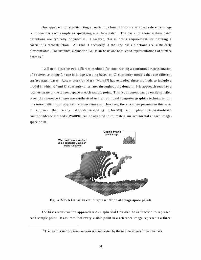
51
One approach to reconstructing a continuous function from a sampled reference image
is to consider each sample as specifying a surface patch. The basis for these surface patch
definitions are typically polynomial. However, this is not a requirement for defining a
continuous reconstruction. All that is necessary is that the basis functions are sufficiently
differentiable. For instance, a sinc or a Gaussian basis are both valid representations of surface
patches10.
I will next describe two different methods for constructing a continuous representation
of a reference image for use in image warping based on C0 continuity models that use different
surface patch bases. Recent work by Mark [Mark97] has extended these methods to include a
model in which C0 and C1 continuity alternates throughout the domain. His approach requires a
local estimate of the tangent space at each sample point. This requirement can be easily satisfied
when the reference images are synthesized using traditional computer graphics techniques, but
it is more difficult for acquired reference images. However, there is some promise in this area.
It appears that many shape-from-shading [Horn89] and photometric-ratio-based
correspondence methods [Wolff94] can be adapted to estimate a surface normal at each image-
space point.
Figure 3-15:A Gaussian cloud representation of image-space points
The first reconstruction approach uses a spherical Gaussian basis function to represent
each sample point. It assumes that every visible point in a reference image represents a three-
10 The use of a sinc or Gaussian basis is complicated by the infinite extents of their kernels.

52
dimensional spherical cloud density located somewhere along the ray determined by the image
point. In three-dimensions this radius could be determined by considering the solid angle
represented at each sample point and the distance of the cloud’s center from the image’s center-
of-projection. A two-dimensional equivalent of this radius calculation can, however, be
computed directly from the warping equation.
The image-space Gaussian reconstruction method described here is a straightforward
adaptation of Heckbert’s Elliptical Weighted Average (EWA) filter [Heckbert89], but it is used in
a forward-mapping algorithm, similar in spirit to the Splatting algorithm described by Westover
[Westover91]. The support of the Gaussian reconstruction function is determined by computing
the change in shape of differential circular regions surrounding each sample as they undergo the
image warp. One useful measure of the change in shape is provided by the Jacobian determinant
of the mapping function. The Jacobian determinant is a direct measure of the local change in
area induced by a transformation. However, changes in differential area are not necessarily a
good indication of the changes in differential shape11. The additional assumptions required to
address this discrepancy will be discussed shortly. The Jacobian matrix of the planar-warping
function given in Equation 3-12 is
J =
+ + − + ++ + +
+ + − + ++ + +
+ + − + +
w w v w w u v w w v w w u v
w u w v w w u v
w w u w w u v w w u w w u v
w u w v w w u v
w w v w w u v w w v w w
11 32 33 34 31 12 13 14
31 32 33 342
12 31 33 34 32 11 13 14
31 32 33 342
21 32 33 34 31 22 23 24
( ( , )) ( ( , ))
( ( , ))
( ( , )) ( ( , ))
( ( , ))
( ( , )) (
δ δδ
δ δδ
δ δ( , ))
( ( , ))
( ( , )) ( ( , ))
( ( , ))
u v
w u w v w w u v
w w u w w u v w w u w w u v
w u w v w w u v31 32 33 342
22 31 33 34 32 21 23 24
31 32 33 342+ + +
+ + − + ++ + +
δ
δ δδ
Equation 3-19: Jacobian of the warping equation
The determinant of the Jacobian matrix simplifies to
∂∂
δδ
( , )
( , )
det( ) ( , ) det( )
( , , ( , ))
′ ′=
+u v
u v
u v
t u v u v
H G3
Equation 3-20: Jacobian determinant of the warping equation
where
11 For instance, consider the mapping { }φ: , .x u y v= =10 0 1 with
∂∂( , )( , ) .x yu v =
=Determinant
10 0
0 0 11. The Jacobian determinant indicates that the differential area
surrounding any sample remains constant; yet the mapping introduces considerable stretching along theu dimension and shrinking in the v dimension.

53
H G=
=
w w w
w w w
w w w
w w w
w w w
w w w
11 12 13
21 22 23
31 32 33
11 12 14
21 22 24
31 32 34
and
Equation 3-21: Camera-model matrix, H, and the structure matrix, G
The H component of the Jacobian determinant represents the change in projected area of an
infinitesimal region of the reference image due entirely to the changes in the pinhole-camera
model since H P P�= −2
11 and det( ( )) det( ) ( , , )JacobianH Hx t u v= 0 3 . The G component
represents the change in projected area due to the three-dimensional structure of the observed
image point. This can be seen by letting H I= , denoting no change in the pinhole camera model
between the reference and desired image. This gives
∂∂ δ( , )
( , ) ( ( , ) )
′ ′=
+u v
u v u v w
1
1 342
indicating that the change in projected area is independent of the point’s coordinate on the
image plane, but instead it depends entirely on the generalized disparity value at that point.
Since the matrices H and G are constant for a given pair of reference and desired views, they
need only be calculated once per warp.
If we make the assumption that the warping function is well represented by a local
linear approximation centered at each sample in the reference image with a constant generalized
disparity value, then the Jacobian matrix can also be used to estimate the change in shape of a
rotationally symmetric reconstruction kernel as follows. An infinitesimal circular region with a
radius of dr is described by the expression
[ ]dr du dvdu
dv2 =
Equation 3-22: Radius of differential region
When that region undergoes an arbitrary mapping, φ:( , ) ( , )u v u v→ ′ ′ , the best linear
approximation to the differential mapping is given by the Jacobian matrix
du
dv
du
dv
′′
=
J
Equation 3-23: Differential change induced by mapping
54
By substituting Equation 3-23 into Equation 3-22, the mapping of the differential circular region
can be determined as follows:
[ ]dr du dvdu
dvT2 1 1= ′ ′
′′
− −( )J J
Equation 3-24: Projection of differential circular disk
which expands to the following conic expression:
drj j du j j j j du dv j j dv
j j j j2 21
2222 2
11 21 12 22 112
122 2
11 22 12 212
2=
+ ′ − + ′ ′ + + ′−
( ) ( ) ( )
( )
Equation 3-25: Expanded expression for differential circular disk
This equation describes an ellipse if the Jacobian determinant is positive. Therefore, any circular
region centered about a reference image sample will project as an ellipse in the desired image.
This property can be used to reconstruct a continuous representation of the reference image
prior to resampling. The spatial domain response of any rotationally symmetric filter, such as a
Gaussian, can be computed at a sample point in the desired image by evaluating Equation 3-25
at that point to determine the radius value in the undistorted filter’s kernel. The resampling
process can be optimized by first computing the extents of the ellipse in the desired image space.
In terms of the Jacobian these extents are given by the following expressions:
∆ ∆′ = ± −
+ −′ = ± −
+ −++
++
udr j j j j
j jv
dr j j j j
j jj j j j
j j
j j j j
j j
211 22 12 21
2
212
222
211 22 12 21
2
112
12211 21 21 22
2
112
122
11 21 21 222
212
222
( )
( )
( )
( )( )
( )
( )
( )
Equation 3-26: Screen-space extent for projected circular disk
Another approach to reconstructing a continuous representation of the reference image
attempts to fit a bilinear surface patch between any four neighboring grid samples. This
representation also has C0 continuity, but it uses a polynomial basis. First, the individual
sample points of the reference image are mapped to the desire image’s coordinate system.
These warped points will generally not correspond to sample grid positions. The connectivity
of the eight-connected neighborhood of each reference sample-point is maintained after the
warp. This can be managed by maintaining a buffer of two scan lines while enumerating the
reference image in a visibility compatible order. The warped sample points stored in these two
buffers can be considered a single strip of patches at the completion of each scan line. A

55
standard polygonal rasterizer can be used to scan convert each patch in the strip. Therefore, this
technique can easily take advantage of specialized rasterization hardware if it is available. Once
a strip is rasterized, one of the scanline buffers becomes available for storing the mapped values
of the next scan line.
Shown below is an example of the same warp using each of the two reconstruction
methods discussed.
Figure 3-16:Example image warps using different reconstruction methods
3.7 Occlusion and Exposure Errors
Only those scene points that are visible in the reference image can be correctly
reprojected by the image warp. In some cases, even the visibility of a point does not guarantee
its proper reconstruction. These are not weaknesses of either the image-warping or visibility
methods described; they are, instead, inherent limitations of an image-based representation.
The major visual artifacts resulting from these limitations can be classified as one of two
cases, exposure errors or occlusion errors. Exposure errors occur when a background region that
should have been occluded is visible in a desired image because of the absence of some
foreground element from the reference image. On the other hand, occlusion errors occur in a
desired image when an interpolation error in the reconstruction process introduces a false
Gaussian Cloud Bilinear Patch

56
foreground element that covers background regions visible in the actual scene. The choice of
reconstruction methods plays a significant role in either amplifying or reducing these errors.
However, a reduction in one class of artifact often causes an increase in the other.
Many exposures and occlusions are correct. For instance, when a viewpoint moves
toward a foreground object the projection of the object will enlarge in the field-of-view such that
it covers adjacent background points. As the viewpoint moves even closer to the foreground
object, more of the background is occluded.
Exposure errors and occlusion errors take place either when the underlying
assumptions of the reconstruction method are violated, or when there is insufficient information
in the image to properly reconstruct the correct surface. These two error sources are closely
related. The role of reconstruction kernel is to interpolate the missing gaps between samples.
Often the information needed to correctly fill a missing image region is unavailable from the
reference image.
Exposure errors are the more subtle visual artifact. The region uncovered by a
legitimate exposure lends itself to interpretation as a shadow produced by a light source placed
at the reference image’s center-of-projection. This is particularly noticeable when the exposure
occurs along object boundaries. An exposure error occurs when a ray in the desired image
passes through this shadow region, allowing some background element to be erroneously seen.
Both exposure errors and actual exposures are illustrated below.
Figure 3-17:Exposures at occluding boundaries
ReferenceImage
DesiredImage
ExposureRegion

57
The actual scene points that are visible from the reference image are shown darkened. The
shaded region indicates where an exposure occurs in the desired image. The solid dividing line
through the exposure region indicates the boundary between an actual exposure to the right and
an exposure error to the left. However, without external information the difference between
valid and invalid exposures cannot be resolved.
Exposure errors are most likely to occur at object silhouettes. They occur on smooth
surfaces as well as along sharp depth discontinuities. This situation is depicted in Figure 3-18.
Exposure errors occur immediately adjacent to those image points who’s ray lies in the observed
object’s tangent plane. Therefore, as an observer moves to see around an object boundary, she
should generally expect to see more of the object rather than any component of the background.
Figure 3-18:Exposure error on a smooth surface boundary
Merely changing the basis function used in the reconstruction of the reference image can
eliminate exposure errors, but it introduces occlusion errors. Consider the example shown in
Figure 3-19 when a polynomial basis, instead of the Gaussian cloud model, is used to
approximate the underlying surface.
ReferenceImage
DesiredImage
ExposureError

58
Figure 3-19:Occlusion errors introduced by polynomial reconstruction
The lighter shaded area indicates the extent of an occlusion error, whereas the darker shaded
area represents an actual occlusion. The surface seen along the occlusion error corresponds to
an extension of the foreground object’s tangent plane. This surface will always enclose the
actual surface. However, it is unlikely that any part of this extension will actually represent a
point in the environment. The occlusion error will usually hide valid exposures. Furthermore,
since occlusion errors are not adjacent to an actual occlusion, they appear more unnatural than
exposure errors.
The continuity of the polynomial interpolation basis causes an excessive estimation of
the number of points in the scene. The polynomial interpolation model reconstructs images that
are indistinguishable from a model that assumes that all of the points beyond each ray’s
observed point are occupied. Such a model will not miss any actual scene points, but it will
erroneously include scene points that do not exist. The polynomial reconstruction method will,
therefore, introduce a disproportionate number of occlusion errors. This can greatly hinder the
usefulness of such a model.
In contrast, the Gaussian reconstruction method represents a vacuous estimate of a
scene’s contents. It assumes that the visible image point is the only scene point located along the
ray’s extent. Therefore, a Gaussian reconstruction basis will correctly represent all empty
regions of an environment, while missing all scene points that are not visible in the reference
image. It is, therefore, conservative in its estimate of the occupied volume of space, whereas the
ReferenceImage
DesiredImage
OcclusionError

59
polynomial reconstruction makes a conservative estimate of the space’s emptiness. Exposure
errors should be expected when the Gaussian reconstruction model is used.
Valid occlusions are generally handled by the visibility algorithm. One exception is the
case when a scene point from outside the viewing frustum comes into view as a result of the
change in the center-of-projection. This situation results in an invisible occluder error. A simple
example of this case is shown in Figure 3-20. This problem is a direct result of the limited field-
of-view available to a planar-pinhole camera. The use of panoramic pinhole-camera models,
such as the ones discussed in the next chapter, will remedy this problem.
Figure 3-20:An external exposure error
The two reconstruction methods discussed previously represent two extreme
assumptions concerning the structure of space. The use of either of these extreme positions
introduces artifacts in the final rendering. A more accurate reconstruction should combine
elements of both methods. However, this might require additional information beyond that
which is deducible from the reference image alone. This is an interesting area for future
research.
3.8 Summary
This chapter has presented a complete example of an image-based method for
synthesizing computer graphics. Special mapping functions, called image warps, were derived
that enabled arbitrary views of a scene to be generated. This scene was represented by a
reference image that was augmented by a scalar value defined at each point, called generalized
ReferenceView Desired
View
InvisibleOccluder

60
disparity. An algorithm was presented to resolve the visibility of the mapped reference points
at each coordinate in the desired image. Two methods were presented for reconstructing
continuous representations of the warped reference image from these warped points. In
subsequent chapters, aspects of this image-warping approach will be generalized and developed
further.

61
&KDSWHU �
OTHER PINHOLE CAMERAS
In Chapter 3 a general model of a planar pinhole camera was introduced in order to
derive and explore the warping equation. This model was particularly well suited to the task
because it lent itself to easy manipulation using linear algebra. Unfortunately, real-world
cameras are not usually specified in this general form. Even if they were, there are
disadvantages in limiting ourselves to image-to-ray mapping functions defined on a plane. In
this chapter I will compare the general model of Chapter 3 to common pinhole-camera
specifications used in other applications. I will also describe a canonical pinhole-camera model
that embodies only those intrinsic properties of a camera that are independent of the coordinate
system in which the camera is specified. The remainder of the chapter discusses non-planar
pinhole cameras that are useful both as representation formats and as distortion models for real-
world imaging systems. I also present specific non-planar extensions to the warping equation,
plus a general methodology for extending the warping equation to any non-planar camera
model.
4.1 Alternative Planar Pinhole-Camera Models
In other application domains the mapping of points on the image plane to rays in space
is described in terms other than the 3 × 3 matrix model used by the general pinhole model of
Chapter 3. The goal of these alternate specifications is to describe the pinhole-camera model
with some minimal set of physically meaningful quantities. Typically, such models are either
nongeneric, admitting only a subset of the mappings achievable with a more general pinhole-
camera model, or overly general, admitting different parameter choices that result in the same
mapping functions. In truth, the 3 × 3 matrix formulation of a pinhole camera is also overly
general because, while it is determined by nine parameters, any scalar multiple describes the
same mapping. Thus, it can have at most 8 true degrees of freedom. In the remainder of this
section several of these application-specific models will be explored and related to the general

62
model. I will also point out the degrees of freedom in each specification and how each
parameterization affects the potential camera geometries that can be expressed.
4.1.1 Application-specific planar pinhole-camera models
The first model considered is one commonly used in computer graphics. It reflects a
viewing plane parallel to two of the given basis vectors. Three parameters are used to specify
the field-of-view, the width, and the height of the viewing plane. The image-space-to-ray
mapping of this simple camera model is
( )( )
( ) ( )
d
d
d
u
vi
j
k
width
height
width fov
=−−
1 0
0 1
0 0 1
2
2
2 2cot
Equation 4-1: A simple pinhole-camera model
where the horizontal field-of-view is given by fov. The terms width and height give the
dimensions of the viewing plane. It can be seen by inspection that this parameterization is a
special case of the general pinhole-camera model. This formulation is only capable of describing
viewing frustums shaped like right pyramids with rectangular bases perpendicular to the basis
vector indexed by k.
�j
�i
�k
fov
width
height
Figure 4-1: Illustration of a simple pinhole-camera model

63
The flexibility of this simple three-parameter model is comparable to an ideal
photographer’s camera12. The horizontal field-of-view of such a camera is determined by the
focal length of the lens, f, and the dimensions of the film plane, as shown in Equation 4-2. For
example, the film plane of a typical 35 mm camera in a landscape orientation is 36 mm wide and
24 mm high. Therefore, a 50mm lens would provide a 39.6° horizontal field-of-view for use in
Equation 4-1.
( )( )fov
w
f
d
d
d f
u
vi
j
k
width
height=
→
=−−
22
1 0
0 1
0 0 1
2
2Arctan
Equation 4-2: Finding an ideal camera’s field-of-view from its focal length
A second pinhole-camera description frequently used in computer graphics is tailored
to a direct specification of the viewing frustum. Its image-space-to-ray mapping function is
given by
d
d
d
left
right
near
u
vi
j
k
right leftwidth
bottom topheight
=
−
−0
0
0 0 1
Equation 4-3: Frustum model of a pinhole camera
In this frustum model the viewing plane is parallel to the first two basis vectors and has a
distance from the origin of near. The boundaries of this viewing plane are determined by the
parameters left, right, top, and bottom, given in image-space units.
12 In all likelihood, a real camera will have a slightly skewed viewing frustum. In addition, it is
also likely to exhibit the angular distortion and finite aperture effects discussed later in this chapter.

64
Figure 4-2: Illustration of the frustum model
This model allows non-symmetric viewing frustums to be specified, permitting off-axis
projections such as those commonly used for multiplexed stereo display. Despite it’s
formulation in terms of five parameters, the frustum model has only four degrees of freedom
since any uniform scaling of all five terms results in the same mapping.
Two real-world examples make use of the frustum model. When a bellows is used, a
photographer’s camera achieves projections similar to the frustum model. Also, the projection
of a cropped photograph must be modeled using the frustum model.
The computer-vision community uses a model of a planar pinhole camera that utilizes
several physically-based quantities in its description. These include the camera’s focal length, f,
the lengths of the image-plane basis vectors, ku and kv, the angle separating these basis vectors, θ,
and the point on the image plane where the optical axis intersects the image plane, (cx, cy).
( )( )
d
d
d
k k c
k c
f
u
vi
j
k
u v x
v y
=−−
cos
sin
θθ0
0 0 1
Equation 4-4: Computer-vision pinhole-camera model
left
right
top
bottomnear

65
This six-parameter model has more flexibility than either of the two computer-graphics
models. It incorporates all of the capabilities of the frustum model with the addition of skewed
spanning vectors in the image plane.
Figure 4-3: Illustration of computer-vision model
In the previous two models the first two columns, which correspond to the &
a and
b vectors of the general model, were orthogonal and therefore independent. In the computer-
vision model the angle θ determines how skewed these spanning vectors are. However, the
computer-vision model is still overly general because different combinations of the f, ku, and kv
terms can give rise to the same camera.
All three alternative planar models make the common assumption that the viewing
plane is parallel to the x-y plane. This family of planes is distinguished by a vector from the
origin toward the viewing plane and perpendicular to both the x-y plane and the viewing plane.
This direction is called the optical axis. In the general planar pinhole model the optical axis is
given by the vector, a b× . In the computer-graphics and computer-vision pinhole-camera
models the optical axis is the z-axis.
The assumption that the viewing plane is parallel to the x-y plane does not limit the
generality of the planar pinhole-camera model, since this condition can always be achieved by
an appropriate choice of coordinate systems. Ideally, one would like to decompose a general

66
pinhole-camera specification into two parts: those characteristics determined by the choice of a
coordinate frame, and the intrinsic properties of the camera.
4.1.2 A canonical pinhole model
In the computer-graphics and computer-vision pinhole-camera models discussed in the
previous section, the coordinate system was conveniently selected in order to simplify the
model’s formulation. This can be accomplished for the general pinhole camera using a QR
decomposition that factors a matrix into the product of an orthonormal matrix, R, and an upper
triangular matrix, U. Geometrically, the orthonormal matrix can be considered a rotation that
aligns the pinhole model to the desirable coordinate frame. The upper-triangular matrix
determines the field-of-view, focal length, optical center, and any other parameters that
influence the shape of the viewing frustum. The elements of U constitute the so called intrinsic
properties of the camera.
The upper triangular matrix, U, of a QR decomposition of the general pinhole-camera model
can be expressed in terms of the three column vectors of P. This results in the expression given
in Equation 4-5, in which R is a three-dimensional rotation matrix, and the vectors a , b , and
c are the columns vectors from the general pinhole-camera-model matrix. Notice that the
rotated pin-hole-camera matrix, U, has the same upper diagonal form as all the previously
discussed pinhole-camera models from computer graphics and computer vision.
d
d
d
a a a ba b
ac
a c
a
a b b b b cb c b c
b
a b c c c c c
u
v ui
j
k
=
′ = ⋅ ′ =⋅′
′ =⋅′
′ = ′ = ⋅ − ′ ′ =⋅ − ′ ′
′′ = ′ = ′ = ⋅ − ′ − ′
=R RU
1 11
11
2 2 12
21 1
2
3 3 3 12
22
0
0 01
Equation 4-5: Deriving a canonical-pinhole camera from a general one
QR decompositions are not unique. In general they come in eight varieties according to
the signs of the square roots appearing on the upper diagonal. If the orthonormal matrix, R, is
limited to rotations, then the number of solutions is reduced to four: those where the signs of the
determinants of the mapping matrix, P, and U agree. From this set of four, there exists only one
decomposition where the two matrix entries, ′a1 and ′b2 , are positive. I will consider this
solution as the canonical representation of U.

67
This transformation has a straightforward physical interpretation. Given the general
configuration depicted in Figure 3-2 there exists a family of rotations that aligns the vector a
with the �i basis vector. For each rotation, there also exists a second rotation about the �i basis
vector which makes the image plane parallel to the plane containing the �i and �j basis vectors.
The composition of these two rotations gives the R matrix, and the resulting coordinates of the
transformed vectors ′a , ′b , and ′c are the columns of the upper-triangular U matrix.
Previously, I have stated that scalar multiples of the general pinhole-camera model
result in the same image-space-to-ray mapping function. This is also true of the canonical
pinhole-camera representation. Thus, a scaling factor can be selected so that the vector a is of
unit length. The resulting U will have the form
U
ba
ca
ba
caca
=
′′
′′
′′
′′′′
1
0
0 0
1
1
1
1
2
1
2
1
3
1
Equation 4-6: A normalization of the canonical pinhole-camera model
The resulting normalized planar pinhole model is determined by five independent
parameters whose values uniquely determine the solid angle of rays captured by the particular
camera. This model can be interpreted physically using the same visualization as the general
pinhole model, P. We can also develop an intuition for reasonable parameter values by
comparing the five parameters to those of the simple pinhole-camera model (Equation 4-1). For
example, one might expect that the ′′
ba
11
term would be nearly 0 and that the ′′
ba
21
term would be
almost 1 for all but the most unusual of cameras.
4.1.3 Planar calibration
The process of off-line camera calibration can be viewed as the determination of the five
unknown parameters of U using observations of known points. In addition an online camera
calibration process also attempts to determine the six parameters of the camera’s pose (its
position and orientation). These pose parameters are often called the extrinsic camera
parameters, and their unambiguous assignment is dependent on the choice of coordinate
frames. In addition to the simple planar pinhole model’s parameters, most calibration
procedures usually attempt to characterize the nonlinearities of the image-space-to-ray mapping
function not described by this simplified model. In the next section I will address this problem
and its impact on the warping equation developed using only the ideal planar model.

68
4.2 Nonlinear Pinhole-Camera Models
The planar pinhole-camera model has some shortcomings which limit its practical use
and make it an inconvenient representation for image-based computer graphics. First, a planar
pinhole camera is only capable of representing a subset of those rays visible from a particular
viewing position. This results from the fact that even an infinite plane subtends only half of
the 4π solid angle visible from a given point. Second, the idealized and mathematically elegant
planar pinhole-camera model does not reflect the true nature of real-world image acquisition
devices.
In this section a series of more general pinhole-camera models will be characterized
which address the problems of the ideal planar model. The first set of generalizations
overcomes the problem of the limited solid angle visible by a planar pinhole camera by
describing the mathematical structure of several panoramic cameras. Next, a series of modified
pinhole models will be discussed that account for the geometric distortions present in real-
world cameras.
The essence of the pinhole camera is the mapping function from image-space
coordinates to rays in a viewing space. In the case of a planar pinhole camera this mapping
function is a linear rational function, easily described by a matrix. The more complicated
models described in this section are algebraic in nature and more difficult to manipulate in
general. However, much of the intuition developed for the linear case can be readily adapted to
these more complicated models.
4.3 Panoramic Pinhole Cameras
I have described image-based computer graphics as a process in which a set of reference
images is used to interpolate, extrapolate, and otherwise model the plenoptic function of a given
visual environment. By fixing both the time and viewpoint, the plenoptic function reduces to a
form that is equivalent to our typical notion of an image. Furthermore, any reference image
used to model a scene represents some subset of such an image.
Our practical experience with images, however, is limited to a surprisingly small
fraction of the visual sphere. The typical 50 mm lens on a 35 mm camera captures less than 3%
of the available solid angle. Even a relatively wide angle 28 mm lens on the same camera
captures just over 7% of the visual sphere. Our visual system, however, incorporates

69
information over a very large visual angle, estimated at about 43% of the visual sphere on
average [Slater93].
The term panoramic is commonly used to describe images with large aspect ratios.
However, its proper definition is “an unobstructed view of an extensive area”. I will use the
term panoramic to describe any image whose field-of-view covers a significant fraction of the
visual sphere. In particular I will consider cameras that cover the full range of at least one of the
two angle parameters of a properly oriented spherical coordinate system to be panoramic. Thus,
an image captured through a fisheye lens would be considered more panoramic than a cropped
aerial image of a city skyline. Unlike a cropped image, a true panoramic image, like any wide-
angle view, usually exhibits significant perspective distortions unless viewed from the
appropriate position.
The motivation for developing warping equations for wide-field-of-view images is that
they are particularly well suited for use as reference images. Their use also provides many
useful simplifications by eliminating boundary cases. The pinhole-camera models described
first in this section are characterized by mapping functions capable of describing larger portions
of the visual sphere than possible with the planar pinhole-camera model. However, like the
planar pinhole model, these wide-field-of-view pinhole-camera models are ideal mathematical
constructions. Thus, in the context of an image-based graphics system, they are perhaps most
useful as an intermediate model representation, rather than as a description for either acquired
source images or synthesized results.
In each of the models that follows all of image-space is considered to be parameterized
over the domain of a unit square. These models map image points to a ray direction in a
Euclidean three-space. If required, an auxiliary pre-warp can be applied to the image-space
coordinates to map the pixel coordinates onto the unit square. Usually, this pre-warp is nothing
more than a scaling of the two pixel coordinates by their extreme values.
Just as the canonical representation of the planar pinhole model provides for the most
compact representation of the camera’s intrinsic properties, similar simplifications can be
applied to non-planar models. The relationship of the canonical model to an arbitrary
representation was merely a choice of an appropriate coordinate system. The coordinate
systems of the non-planar mapping functions can also be selected such that their expression is in
terms of some minimal number of parameters. A post-warp rotation can be applied to orient

70
the canonical frame to any desired orientation. All of the following pinhole-camera models are
presented in their canonical forms and defined over the domain of a unit square.
4.3.1 Cylindrical pinhole-camera model
In a cylindrical imaging geometry only one of the two image-space dimensions is
sampled over the full range of possible angles. Thus, a cylindrical camera, like the planar
model, is also only capable of representing a subset of the visual sphere. However, the solid
angle subset that can be represented by cylindrical geometry does asymptotically approach the
full 4π range, whereas a planar geometry can, at best, represent only 2π. The following three-
parameter model can be used to specify a canonical cylindrical mapping:
( )( )
( )d x
u k v
y y y v
u k v
u vcylinder
o
cylinder
= =+
+ −+
∈C( )
sin
cos
, [ , ]
2
2
0 11 0
π
π
Equation 4-7: Canonical cylindrical mapping function
The panoramic nature of the cylindrical pinhole-camera model actually reduces the
number of intrinsic camera parameters required for its concise specification, as illustrated in
Figure 4-4. Two of the parameters, and y1 , control the vertical field of view. The remaining
parameter, kcylinder , behaves similarly to the skew parameter of the planar model.
Figure 4-4: The canonical cylindrical pinhole-camera viewing surface
y0
y1
k
i
j

71
In this canonical representation the cylinder’s axis is aligned with the �k basis vector.
The skew parameter in the figure shown is nearly zero, as reflected by the perpendicular
orientation of the isoparametric lines shown on the viewing surface. Unlike the planar pinhole-
camera case, the skew parameter has no effect on the shape of the solid angle acquired by the
camera. Therefore, for each cylindrical-pinhole camera, there exists an equivalent camera, in
terms of the solid angle sampled, for which the value of kcylinder is 0. Such a camera
configuration can be achieved with an appropriate linear prewarp as shown below:
′′
=
−u
v
u
v
kcylinder1
0 12π
Equation 4-8: Prewarp to remove skew parameter from a cylindrical mapping function
The inverse of the cylindrical mapping function maps a given ray’s direction to an
image-space coordinate. The expression for this mapping function is given in Equation 4-913.
x d
dxdz cylinder
dy
dx dz
y
y y
d y
dx dz
k
y
y y= =
−
−
−
−
+−
−
+C 1
2
2 20
1 0
2 2 0
1 0
1
( )
( )Arctan
π
Equation 4-9: Inverse of the cylindrical mapping function
A cylindrical viewing surface has several practical advantages when used as a plenoptic
sample representation. Since a cylinder is a developable surface it can easily be represented in a
computer’s memory using a two-dimensional array. Also, since the angular sampling density is
constant around the cylinder’s circumference it is a slightly more efficient representation than a
planar projection. But the most significant advantage of the cylindrical viewing surface is that it
is relatively simple to acquire such projections by reprojecting planar images acquired when a
camera that is rotated on a tripod [Mann94], [Chen95], [McMillan95c]. The following figures
represent projections acquired from cylindrical pinhole cameras:
13 I am choosing to maintain the homogeneous representation of image-space points so that
subsequent projective transforms might be applied.

72
Figure 4-5: A cylindrical pinhole model of an operating room scene
Figure 4-6: A cylindrical pinhole model of Sitterson Hall
Figure 4-7: A wide-angle cylindrical pinhole model of the old well
The image-warping equation can easily be adapted to use the cylindrical pinhole-camera
model. The relationship of the image-space coordinates of a point that is seen in two images is
given by
C C1 1 0 0 1 0 0( ) ( )( � � ) ( )x x C C x= − +δ
Equation 4-10: Cylinder-to-cylinder correspondence
Note the similarities between Equation 4-10 and the planar mapping of Equation 3-4.
The derivation of the warping equation for the cylindrical camera is more complicated than in
the planar case, since the mapping functions are nonlinear and must be manipulated as algebraic
expressions instead of linear algebra. The resulting cylinder-to-cylinder warping equation is
given by
( )x x C C x1 11
0 0 1 0 0= − +−C Cδ( )( � � ) ( )
Equation 4-11: Special cylinder-to-cylinder warping equation

73
In this expression the two pinhole cameras are defined independently; however, their
basis vectors are assumed to be parallel. A more general version of the warping equation is
required when the basis vectors are not aligned.
( )x x C C a x1 11
0 0 1 0 0= − +−C R Cδ θ( )( � � ) ( �, ) ( )
Equation 4-12: General cylinder-to-cylinder warping equation
In the equation above R( �, )a θ is a three-dimensional rotation matrix about the axis �a by an angle
of θ , defined in the coordinate system of the reference image with an origin of �C0 . Any other
parameterization of a three-dimensional rotation can also be used.
When both cylindrical pinhole-camera models are known to have the same intrinsic
parameters and are defined with parallel basis vectors, the warping equation can be simplified
to
x x C C C x
x
k v
v
u k v u v C C
u k v u v C C cylinderu v C C
y y
u v C C
y y
cylinder x x
cylinder z z
y y
y y
11
0 0 1 0
1
12
0 1
0 1
0 1
1 0
0 1
1 0
1
= − +
=
− +
+
−
+ + −+ + −
−−
−−
C ( ( )( � � ) ( ))
) ( , )( )
) ( , )( )
( , )( )
( , )( )
δ
ππ δπ δ
δ
δ
Arctansin(2
cos(2
Equation 4-13: Aligned cylinder-to-cylinder warping equation
If the cylinder’s skew parameter is zero, the warping equation further simplifies to
( )x v
u u v C Cu u v C C
u v C C
y y
x x
z z
y y
1
12
0 1
0 1
0 1
1 0
1
=
+
+ −+ −
−−
ππ δπ δ
δ
Arctansin(2cos(2
) ( , )( )) ( , )( )
( , )( )
Equation 4-14: Aligned cylinder-to-cylinder warping equation without skew
Just as in the planar-warping equation, the cylindrical-warping equation specifies a
mapping of points from the reference image to their positions in a desired image. The warp is
controlled by a generalized-disparity parameter that is specified at each point of the reference
image. When the center-of-projection of the desired image coincides with the center-of-
74
projection of the reference image, the warping equation reduces to the reprojection case as
follows:
( )x a x1 11
0 0= −C R C( �, ) ( )θ
Equation 4-15: Cylinder-to-cylinder reprojection
As mentioned previously, panoramic images are particularly useful as reference image
representations. The cylinder-to-cylinder warping function described above can be used to
accomplish such mapping. Typically, though, the desired image will be a planar projection. It is
possible to re-project the results of the cylinder-to-cylinder mapping onto the desired viewing
plane directly.
( )x x C C x1 11
0 0 1 0 0� ( )( � � ) ( )= − +−P Cδ
Since the inverse of the planar-mapping function is linear, it can be distributed across
the sum as shown in the following equation:
x x C C x1 0 11
0 1 11
0 0� ( ) ( � � ) ( )= − +− −δ P P C
Equation 4-16: Cylinder-to-plane warping equation
This expands to the following rational expressions:
( ) ( ) ( )( ) ( ) ( ) ( )( ) ( ) ( )( ) ( )u
b c b c u kv b c b c u kv b c b c y y y v C C b c u v
a b a b u kv a b a b u kv a b a b y y y v C C
y z z y x y y x z x x z
y z z y x y y x z x x z
1
0 0 0 0 0 1 0 0 0 1 0 0
0 0 0 0 0 1 0 0 0 1
2 2
2 2=
− + + − + + − + − + − ⋅ ×
− + + − + + − + − + − ⋅
( ) sin ( ) cos ( ) � � ,
( )sin ( ) cos ( ) � �
π π δ
π π ( ) ( )
( ) ( ) ( )( ) ( ) ( ) ( )( ) ( ) ( )( )
a b u v
vc a c a u kv c a c a u kv c a c a y y y v C C c a u v
a b a b u kv a b a b u kv a b a b y y y v
y z z y x y y x z x x z
y z z y x y y x z x x z
×
=− + + − + + − + − + − ⋅ ×
− + + − + + − + −
δ
π π δ
π π
0 0
10 0 0 0 0 1 0 0 0 1 0 0
0 0 0 0 0 1 0 0
2 2
2 2
,
( ) sin ( ) cos ( ) � � ,
( ) sin ( ) cos ( ) ( ) ( ) ( )+ − ⋅ ×� � ,C C a b u v0 1 0 0δ
Equation 4-17: Expanded cylinder-to-plane warping equation
This equation can be used to map the points of a cylindrical pinhole-camera model to any
viewing plane. Consider the following example of a cylindrical projection.

75
Figure 4-8: A cylindrical projection
The cylindrical projection shown above was assembled by first registering 12 planar
projections and then reprojecting them onto a cylindrical viewing surface using Equation 4-14
[McMillan95c]. These planar projections were themselves reprojections of acquired images that
were captured using a fish-eye lens and reprojected using a nonlinear pinhole-camera model
discussed in the next subsection. The following projections demonstrates the use of the
cylinder-to-plane warping equation given in Equation 4-17.
Figure 4-9: Desired images from a cylinder-to-plane warp

76
Each of the four images shown in Figure 4-9 result from a cylinder-to-plane warp of Figure 4-8.
The lower boundary of the cylindrical viewing surface is clearly visible in the lower-left image.
4.3.2 Spherical model
A spherical imaging geometry spans the full range of both angle parameters. It
therefore represents the entire 4π visual angle and a complete pencil of rays. The spherical
pinhole-camera model has fewer intrinsic parameters than any other model. The following one
intrinsic-parameter mapping function describes the canonical spherical pinhole camera:
� ( )
sin( ) sin
cos
cos( ) sin
, [ , ]d x
u k v v
v
u k v v
u vsphere
sphere
= =+
+
∈S
2
2
0 1
π ππ
π π
Equation 4-18: Spherical mapping function
Once more, the intrinsic spherical skew parameter, ksphere, is similar to the planar skew
factor; when it is zero, the isoparametric curves intersect at right angles. The intrinsic skew
parameter does not, however, have any effect on the solid angle represented by the mapping
function. Therefore, it can also be made zero with a suitable prewarp.
′′
=
−u
v
u
v
ksphere1
0 12π
Equation 4-19: Prewarp to remove spherical skew
The viewing surface of the canonical spherical mapping function is shown below with a
skew value of zero.
Figure 4-10:The viewing surface of the canonical spherical pinhole-camera model

77
The cutout allows the basis frame of the ray-space, as well as the image-space basis
frame, to be seen. The image-space parameterization of the spherical camera model is non-
uniform in its solid angle coverage. While none of the pinhole cameras discussed thus far
(planar or cylindrical) realize a uniform sampling of the solid angle, the spherical geometry is
notable in its deviation. A side effect of this nonuniform coverage is that any image-space
presentation of a spherical projection appears geometrically distorted. This is especially
noticeable around the poles of the projection. Furthermore, the lack of uniformity is somewhat
surprising since the image-space parameters are directly related to planar angle values.
The inverse of the spherical mapping function is given by the following expression:
( )( )
x d
k
dxdz
dx dzdy
dx dzdy
sphere
= =
−
−
+
+S 1
2 2
2
2 2
2
2 2
1
( �)
ArctanArctan
Arctan
π π
π
Equation 4-20: Inverse spherical pinhole-camera model
The spherical pinhole-camera model can also be used as a mapping function in the
warping equation. A general treatment of the process for modifying the warping equation will
be discussed at the end of this section.
4.4 Distorted Pinhole-Camera Models
The second group of nonlinear pinhole cameras discussed are significant because they
characterize realizable imaging systems rather than mathematical abstractions. A researcher is
likely to run into one of these camera models when capturing wide-angle images for use in an
image-based graphics system. They can even be considered for use as reference image
representations in real-time systems [VTV96].
The pinhole-camera models explained in this section are often associated with geometric
distortion models. In optics, computer vision, or computer graphics the term geometric distortion
is used to indicate deviations from a standard projection model that are manifested as shape
discrepancies of the depicted object. The difficulty in defining distortions comes in the selection

78
of a standard projection model. The most common choice is a planar pinhole model. The
advantages of the planar pinhole model include a precise mathematical description and the
model’s preservation of certain geometric invariants, such as collineation (the preservation of
lines). However, even planar pinhole images captured at extremely wide angles exhibit
perspective distortions when viewed from a point other than the original center-of-projection.
This phenomenon is largely perceptual. One hypothesis [Zorin95] suggests that the visual
system attempts to interpret uniform spacing in the image plane as a constant angular variation.
Regardless of the perceptual ramifications, the planar model’s non-uniform sampling of solid
angles leads to shortcomings in its use for representation.
Planar projections are sampled more densely, in the angular sense, around the periphery
of an image than in the image’s center. This leads to a wasteful representation when used as a
reference image because, as the field-of-view is extended, the number of additional samples
grows faster than the solid angle covered by those samples. The nonuniformity of this sampling
pattern and its associated distortion pattern is illustrated in Figure 4-11.
Figure 4-11:Wide-angle distortion from a 100° field-of-view planar projection
Figure 4-11 depicts a 7 × 5 grid of regularly spaced spheres as seen through a planar
pinhole camera with a 100º field-of-view. The superimposed grid indicates an angular spacing
of 10º. In general only the spheres nearest the center appear spherical. This perceptual artifact
can be eliminated by viewing the figure at a distance of approximately 1.68 inches with a single

79
eye. The increased grid size near the periphery of the image indicates that those regions are
over-sampled.
Nonlinear pinhole-camera models can come closer to a uniform sampling of solid
angles. The cylindrical pinhole model achieves uniform sampling along one of the angular
dimensions, as illustrated in Figure 4-12. In this figure the same 7 × 5 grid of spheres is shown
viewed through a 100º field-of-view cylindrical projection whose axis is aligned with the vertical
axis of the page. The even spacing of the horizontal grid reflects a uniform angular sampling in
the horizontal direction.
Figure 4-12:A cylindrical projection with a 100° field-of-view
The apparent curvature of the vertical grid is indicative of the fact that a cylindrical
pinhole camera does not preserve lines, except those parallel to the cylinder axis. The shape of
the center row of spheres in this image appears less distorted than the planar case; however,
distortion is still visible along vertical columns.
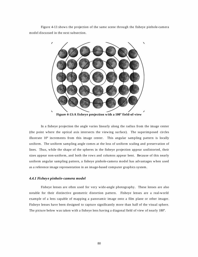
80
Figure 4-13 shows the projection of the same scene through the fisheye pinhole-camera
model discussed in the next subsection.
Figure 4-13:A fisheye projection with a 100° field-of-view
In a fisheye projection the angle varies linearly along the radius from the image center
(the point where the optical axis intersects the viewing surface). The superimposed circles
illustrate 10º increments from this image center. This angular sampling pattern is locally
uniform. The uniform sampling angle comes at the loss of uniform scaling and preservation of
lines. Thus, while the shape of the spheres in the fisheye projection appear undistorted, their
sizes appear non-uniform, and both the rows and columns appear bent. Because of this nearly
uniform angular sampling pattern, a fisheye pinhole-camera model has advantages when used
as a reference image representation in an image-based computer graphics system.
4.4.1 Fisheye pinhole-camera model
Fisheye lenses are often used for very wide-angle photography. These lenses are also
notable for their distinctive geometric distortion pattern. Fisheye lenses are a real-world
example of a lens capable of mapping a panoramic image onto a film plane or other imager.
Fisheye lenses have been designed to capture significantly more than half of the visual sphere.
The picture below was taken with a fisheye lens having a diagonal field of view of nearly 180°.

81
Figure 4-14:A fisheye (left) and planar (right) projection of a yard scene
The mapping of a point on the fisheye imaging surface to a ray direction vector is
nonlinear in terms of image-space coordinates. However, this fisheye mapping function is linear
with respect to the angle between the ray and the optical axis14. An ideal fisheye pinhole-camera
model is described by the following mapping function:
( )�
( ) ( )
tan ( ) ( )
, [ , ]d F x
u u
v v
u u v v
u u v v
u v= =
−
−
− + −
− + −
∈
0
0
02
02
02
02
0 1
κ
κ
Equation 4-21: Fisheye distortion mapping function
A fisheye pinhole camera maps half of the visual sphere (the equivalent to an infinite
plane) onto a disk of radius πκ2 . If appropriately designed, the imaged angle may even extend
outside of this disk. The viewing surface of a fisheye pinhole camera is shown below with
isoparametric lines overlaid.
14 Fisheye projections are often confused with spherical central projections where, at most, a
single hemisphere of solid angle is mapped to a plane, and the angular sampling density is proportional tosin θ rather than linear with θ.
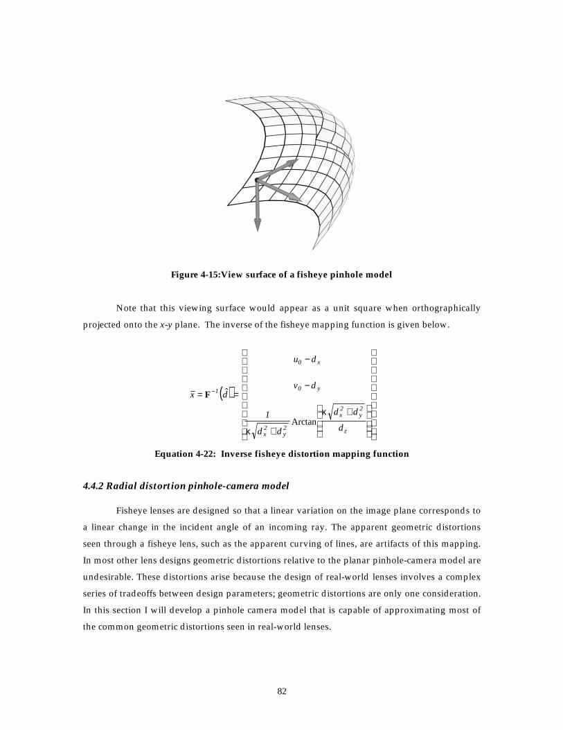
82
Figure 4-15:View surface of a fisheye pinhole model
Note that this viewing surface would appear as a unit square when orthographically
projected onto the x-y plane. The inverse of the fisheye mapping function is given below.
( )x d
u d
v d
d d
d d
d
x
y
x y
x y
z
= =
−
−
+
+
−F 1
0
0
2 2
2 21
�
κ
κArctan
Equation 4-22: Inverse fisheye distortion mapping function
4.4.2 Radial distortion pinhole-camera model
Fisheye lenses are designed so that a linear variation on the image plane corresponds to
a linear change in the incident angle of an incoming ray. The apparent geometric distortions
seen through a fisheye lens, such as the apparent curving of lines, are artifacts of this mapping.
In most other lens designs geometric distortions relative to the planar pinhole-camera model are
undesirable. These distortions arise because the design of real-world lenses involves a complex
series of tradeoffs between design parameters; geometric distortions are only one consideration.
In this section I will develop a pinhole camera model that is capable of approximating most of
the common geometric distortions seen in real-world lenses.

83
Rotational symmetry is common to all of the elements in a typical compound lens
design. This symmetry dictates that the pattern of geometric distortion, as well as most other
lens attributes, will vary radially from the point that the system’s central axis projects onto the
image plane. The variations from an ideal pinhole camera seen in the image plane are usually
modeled in terms of their spatial frequency using Fourier analysis. Because of the lens-system’s
symmetry, only the odd (sine) terms are involved in these models. It is common to consider only
the first three terms of a Taylor series expansion in the summation of these additive effects
[Smith92]. This results in a simple cubic radial-distortion model of the form ′ = +r r r( )1 2κ . This
simple model can be used to accurately model the common pincushion (κ > 0) and barrel (κ < 0)
geometric distortions that are frequently seen in real-lens systems [Tsai87].
Figure 4-16:Two images exhibiting radial distortion.
In the figure above a slight pincushion distortion is visible in the telephoto (narrow
field-of-view) projection shown in left image. The wide-angle projection shown in the right
image exhibits noticeable barrel distortion.
The following image-space-to-ray mapping function (a.k.a. pinhole-camera model) can
be used to model a radial cubic distortion:
( )�
(( ) ( ) )
, [ , ]d x
u u
v v
u u v v
u v
o
= =
−
−
+ − + −
∈R
0
0
20
2
1
1
0 1
κ
Equation 4-23: Cubic distortion mapping function
Viewing surfaces for a cubic distortion pinhole-camera model that is capable of representing
both barrel and pincushion distortions are illustrated in Figure 4-17. The concave surface
relative to the center-of-projection will produce a barrel distortion pattern. The convex surface
produces a pincushion distortion.
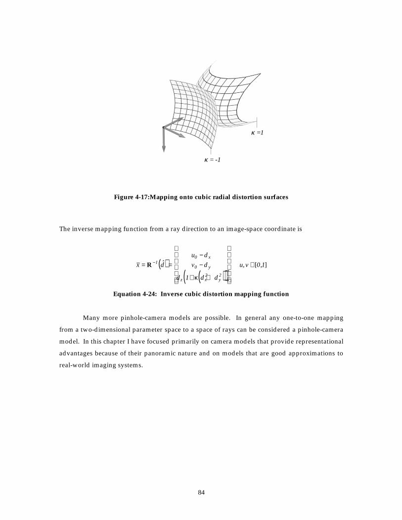
84
Figure 4-17:Mapping onto cubic radial distortion surfaces
The inverse mapping function from a ray direction to an image-space coordinate is
( )( )( )
x d
u d
v d
d d d
u vx
y
z x y
= =−−
+ +
∈−R 10
0
2 21
0 1� , [ , ]
κ
Equation 4-24: Inverse cubic distortion mapping function
Many more pinhole-camera models are possible. In general any one-to-one mapping
from a two-dimensional parameter space to a space of rays can be considered a pinhole-camera
model. In this chapter I have focused primarily on camera models that provide representational
advantages because of their panoramic nature and on models that are good approximations to
real-world imaging systems.
κ = -1
κ =1

85
4.5 Modifying Warping Equations
To this point, warping equations have been derived for the following pinhole camera
configurations:
• plane-to-plane
• cylinder-to-cylinder
• cylinder-to-plane
In this section a general methodology is developed that allows a disparity-augmented
reference image with its associated pinhole-camera model to be warped to a desired image
using any other pinhole-camera model. The only requirements on these pinhole-camera models
are that their mapping functions be one-to-one (each image-space point maps to a unique ray
and vice-versa), and that both a forward projection (image-space to ray) and an inverse
projection (ray to image-space) mapping can be specified. These conditions are satisfied by all
of the pinhole cameras discussed to this point.
The coordinate of a point, �X , in a Euclidean three space is
� � ( ) � ( )X C M x C M x= + = +0 0 0 1 1 1α β
where M x0 ( ) and M x1( ) are the mapping functions from image coordinates to ray directions.
These mapping functions may, or may not, use the same pinhole-camera model. As in the
planar case, the terms �C0 and �C1 represent the three-space coordinates of the respective cameras’
centers-of-projection. Isolating the projective mapping function about �C1 gives
M M1 11
0 1 0 0( ) ( � � ) ( )x C C x= − +βαβ
By scaling both sides by βα , which takes advantage of the fact that a ray’s direction is
independent of its scale, and then defining δ α( )x01= , to indicate α’s dependence on the
parametric coordinate x0 , and computing the inverse-projective mapping of both sides, the
following warping equation results:
x x C C x1 11
0 0 1 0 0= − +−M M( ( )( � � ) ( ))δ
Equation 4-25: General geometrically consistent warp

86
This general equation can be used to map points specified in one image-space to any other. This
includes the process of reprojection where both the source and destination images share a
common center-of-projection.
4.6 Real cameras
The projection and warping approaches used in this chapter, while more general than a
planar pinhole-camera model, are still only approximations to real-world imaging systems.
Parametric mappings onto viewing surfaces, via nonlinear pinhole cameras, are adequate
models for geometric distortions in the image plane. However, pinhole models are still unable
to describe many of the artifacts commonly found in images.
The assumption that all rays collected on the viewing surface originate (or pass through)
a single point in space is the most obvious simplification made in the pinhole-camera model. It
is this property that gives a pinhole camera its name. In real imaging systems the rays pass
through a finite aperture stop. Points on the viewing plane correspond to a weighted average of
all of the rays passing through this aperture. Therefore, there is no single mapping of points on
the image plane to rays in space. It is this property of real lenses that creates depth-of-field (i.e.,
objects at different ranges appear in various degrees of focus). In a true pinhole camera all
points are in sharp focus.
Another deviation between real cameras and ideal pinhole models is the existence of a
lens for the purpose of bending and focusing light. The light-bending ability of a lens is a result
of its refractive properties. Refraction results from the fact that the speed at which light
propagates through non-conductive materials varies depending on the materials’ properties.
The propagation speed through a material also depends on the wavelength of the incident light
energy. Since the various colors of the spectrum are distinguished by their difference in
wavelengths, the refraction of light by lenses introduces color shifts on the viewing surface.
This phenomenon is called chromatic aberration. Optical designers go to great lengths to select
lens materials and designs in order to minimize this effect. In an ideal pinhole camera,
variations due to wavelength are completely ignored, whereas in reality diffraction would come
into play.
4.6.1 Nonlinear camera calibration
As discussed earlier, the problem of determining either or both the intrinsic and
extrinsic parameters of a pinhole-camera model from a set of image-space observations is called

87
camera calibration. By extending the definition of pinhole cameras to include nonlinear models,
distortion parameters can also be determined in the calibration process. There are many
different approaches to calibration.
One of the most popular approaches includes global optimizations based on an all
encompassing model in which distortion and intrinsic parameters are simultaneously solved for
[Tsai87]. A second approach involves a series of reprojections in which distortion parameters
are first computed based on the preservation of known projective invariants (for example, the
preservation of lines or quadrics curves). Once the distortion parameters are found, the
rectified image is then reprojected to a planar viewing surface, and the intrinsic planar
parameters are found [Lenz87]. The third approach involves a tabular mapping from image-
space to rays. This approach is data intensive yet very flexible. Table-based calibration
approaches usually require interpolation from a non-uniform sparse collection of data points.
An additional difficulty of this approach arises when an inverse mapping is required.
4.7 Summary
This chapter presented several generalizations of the image-to-ray mapping functions
that were assumed in Chapter 3. The general planar pinhole camera that was presumed when
deriving the warping equation was first related to planar pinhole-camera models used in other
applications. A canonical planar pinhole-camera model was then introduced that isolates the
distinguishing characteristics of a camera from the coordinate frame in which the camera is
defined. Among these characteristics are five parameters that describe a viewing frustum and
the skew and aspect ratio of the viewing plane.
A series of nonlinear pinhole cameras were next defined. These had practical
advantages over the planar pinhole models because they represented a larger portion of the rays
seen at a given point. The panoramic nature of these camera models reduces the number of
intrinsic parameters required for the pinhole camera’s description, resulting in fewer parameters
to be estimated in the calibration process. Another family of nonlinear pinhole cameras was
defined that emulates the geometric distortions typical of real-world imaging systems. The
general image-based computer graphics approach was extended to incorporate these nonlinear
models.

88
&KDSWHU �
WARPING WITHOUT CALIBRATION
Previously, I have discussed how an image that has been augmented with generalized-
disparity information can be warped to produce projections from different viewpoints. Initially,
these warps were developed for images projected onto planar viewing surfaces, and
subsequently this result was generalized to arbitrary viewing surfaces. All of these warps
required the specification of both the reference and the desired centers-of-projection. In
addition, the pinhole-camera models for both images were needed. In this chapter, I will
discuss how to perform these warps when knowledge about the centers-of-projection and the
camera models (i.e., the calibration information) is unavailable. I begin by introducing a
geometric structure called an epipolar geometry which establishes image-to-image relationships
that are constrained by an underlying three-dimensional geometry. Then, I relate this epipolar
geometry to the planar-warping equation, and I demonstrate how an epipolar geometry can be
used to determine image warps in the absence of predefined calibration information.
I consider only the planar-pinhole camera model. This greatly simplifies the discussion
and allows for the simple manipulation of expressions using linear algebra. However, most of
the developments presented can be generalized to nonlinear camera models, although the math
is more complicated. Moreover, the intuitions developed are directly transferable between the
various cases.
5.1 Epipolar Geometries and the Fundamental Matrix
The rays of one perspective image are seen as a family of lines that intersect at a
common image-space point when viewed from the center-of-projection of a second image.
Likewise, the rays of this second view define a similar structure in the first image. As illustrated
in Figure 2-4, any two centers-of-projection and a ray from either one of them defines a planar
subspace. The projection of such a plane forms a line on each image. If the two centers-of-

89
projection are fixed and every ray from one source is considered, an entire family of planes is
defined. This set of planes, which is given the formal name axial pencil, will project onto each
image as a family of lines called a linear pencil. The set of all planes sharing a line passing
through two centers-of-projection is called the epipolar geometry of the camera configuration.
Figure 5-1: An epipolar geometry
The existence of this geometric structure has significant ramifications. For example, any
general point in an image will determine a line in a second image. Also, the three-space point
visible at a selected image-space point will lie on a specific line in the second image. In other
words, a point in one image determines a ray in space along which a three-space point can be
seen. Generally, that ray will project elsewhere as a line intersecting the projection of this visible
point. The exception to this relationship occurs when the image-point’s ray lies on the line
connecting the two centers-of-projection. This ray will project to a point in both images. Such
points are called epipoles. There are exactly two antipodal rays on the line connecting the
centers-of-projection, each defining two epipoles. In a planar projection, only one of these two
epipoles can be visible because the solid angle subtended by a plane is limited to 2π steradians.
When the epipole’s direction is toward the second camera’s center-of-projection, it represents
the origin of the ray bundle. If the epipole’s direction is away from the second camera’s center-
of-projection, it represents a vanishing point of the ray bundle. The type of the epipole (origin
vs. vanishing point) can be determined from correspondence information.
�C1
�C2

90
Figure 5-2: A camera shown with rays converging towards a vanishing point.
The figure above illustrates both types of epipoles. The left and right grids, as well as
the overall image, are computed from a common center-of-projection projected onto a
cylindrical viewing surface with a 270° horizontal field-of-view. The inset image shows these
grids, the center-of-projection, �C , and the camera from a distance using a planar viewing
surface. The image indicated by the left grid sees the rays of the camera as emerging from the
camera’s center-of-projection. The image represented by the right grid shows the same set of
rays converging towards a common vanishing point. The rays only tend toward this point of
convergence; they will never actually reach it.
5.1.1 The Fundamental Matrix
In this subsection, I present an analytical description of an epipolar geometry called the
fundamental matrix. I will also discuss the properties of this fundamental matrix and methods
for determining it. Most of the results presented here are well known within the computer-
vision community. They are presented here primarily for completeness and as background for
readers who are unaware of the work in this area.
An image-space equation of a line is given by an expression of the form
l x Au Bv CT = + + = 0
Equation 5-1: The equation of a line in image space

91
Any 3 × 3 linear transformation can be used to map image points to lines defined on the
same or some other image plane. Such a mapping is called a correlation15, and it has the form
l x
A
B
C
r r r
r r r
r r r
u
v=
=
R or11 12 13
21 22 23
31 32 33 1
Equation 5-2: A correlation mapping points to lines
Like projective maps, which are called collineations, correlations are only defined down
to a non-zero scale factor. This can be proven by showing that the points of a given line are not
changed when the line’s coefficients are multiplied by a non-zero scale factor. Since the
coefficients of the line result from a product of a point and a correlation, any scaling of the
correlation merely scales the line’s coefficients. Therefore, a correlation has no more than eight
degrees of freedom rather than the nine suggested by its matrix formulation.
An epipolar geometry is a special form of a correlation. Since all of the lines produced
by an epipolar geometry intersect at a single point called the epipole, e , the transpose of the
correlation matrix will have the epipole’s coordinate in its null space16. Therefore, the
correlation will be singular and, in general, it will have a rank of two. This linear relationship
describing epipolar geometries has been studied extensively by Faugeras [Faugeras92a] and
Hartley [Hartley92]. They have given the name fundamental matrix to those correlations that
describe epipolar geometries. The rank requirement of the fundamental matrix reduces the
number of degrees of freedom from eight to, at most, seven.
Fundamental matrices map points from one image space to lines in another. This
mathematical tool is consistent with our application in which points on one image plane
represent rays whose projection onto other viewing planes are lines. I will use the following
notation for representing fundamental matrices: Fba will represent the mapping of points
defined on image plane a, xa , to lines on image plane b, lb .
15 Formally, a correlation is a mapping of an n-dimensional projective point to a hyperplane of
dimension n-1. In the case of an image plane, n = 2, the hyperplane has 1 dimension and is, therefore, aline.
16 ( )R Rx e x eT T T= = 0 for all x . Thus, R Te = 0 .

92
l xb ba a= F
Equation 5-3: Fundamental matrix mapping a point to a line
In the geometric description of epipolar geometries at the beginning of this section, I
mentioned that the rays in one image plane, in conjunction with a second center-of-projection,
determine a set of planes as illustrated in Figure 5-1. The epipolar geometries between these
two images are, therefore, not independent but related by this set of planes (i.e., there is a one-
to-one mapping of epipolar lines in one image to the epipolar lines in the second). The
fundamental matrices between any two image planes are related by the following expression:
F Fab baT=
Equation 5-4: Reversing the fundamental matrix mapping
This is easily proven since, for any two corresponding points xa and xb ,
( )F x x x F xba aT
b aT
baT
b= = 0
and taking the transpose gives
( )x F x x F x F x xaT
baT
b
T
bT
ba a baT
bT
a= = =( ) 0
Therefore, F Fab baT= .
A more constrained formulation of the fundamental matrix that represents the 7
available degrees of freedom, rather than the 9 degrees of freedom available in a 3 × 3 matrix, is
frequently useful. The coordinates of the epipoles from the two images are a natural way of
specifying four of the seven parameters of a fundamental matrix. The coordinates of the
epipoles can be found by solving for the point contained in the null space of the original
fundamental matrix and for the null-space point in its transpose. The following
parameterization can be used to describe any fundamental matrix that has been scaled such that
f f f f11 22 12 21 1− = .
F
e
e
e
e q r
e e
q r e
e
u
v
u
v
u v
q
u
v
21
1
1
2
2
2 2
1
1
11 1
1
0
0
10
1 0
0 1
=
− −
−
−
−
, , , ,cos sin
sin cosθ
θ θ
θ θ
Equation 5-5: Parameterization for a general fundamental matrix

93
where q , r , and θ are the remaining three parameters of the fundamental matrix.
Any matrix of the form given in Equation 5-5 will satisfy the requirements of a
fundamental matrix. In addition, any general fundamental matrix can be decomposed into this
form by first solving for the epipoles. Then, the upper-left 2 × 2 submatrix is scaled by the
reciprocal of the square-root of its determinant, and, finally, the QR decomposition of this
submatrix is computed.
This 7-parameter model serves as a useful symbolic representation of fundamental
matrices in derivations because it maintains the proper number of degrees of freedom while
retaining a form that can be managed with linear algebra. This model can also be used to solve
for a particular instance of a fundamental matrix using any global optimization method, like the
approach discussed in [Luong93b], without any external constraints.
5.1.2 Determining a Fundamental Matrix from Point Correspondences
An epipolar geometry describes image-space relationships that are implicitly coupled to
a three-dimensional geometric structure (i.e., the axial pencil of planes through the line
connecting the centers-of-projection of two images). This subsection describes how a general
fundamental matrix can be derived based entirely on image-space relationships. In this way,
three-dimensional geometric constraints can be implicitly placed upon image-space quantities.
A fundamental matrix can be found using linear methods when the coordinates for
eight corresponding points on two different image planes are given (A closely related result was
first presented by Longuet-Higgins [Longuet-Higgins81]). Each pair of points specifies one
equation as shown below.
x x
u u f u v f u f v u f v v f v f u f v f f
T2 21 1
2 1 11 2 1 12 2 13 2 1 21 2 1 22 2 23 1 31 1 32 33
0
0
F =
+ + + + + + + + =
Equation 5-6: Linear equation in the coefficients of a fundamental matrix
This equation is linear in terms of the coefficients, f ij , of the fundamental matrix, F .
An 8 × 8 system of linear equations with nine unknowns can be established by considering the
equations generated by all eight corresponding points.

94
Af = 0
Equation 5-7: Linear homogeneous system
A fundamental matrix can be scaled such that any one of its nine coefficients is exactly
equal to one. This allows the column of A to be moved to the right side of the expression. The
resulting matrix, ′A , will be square, and the equation will, in general, be nonhomogeneous. An
element could be chosen at random and a solution could then be found for all cases except when
the selected element is actually zero. Alternatively, the nonlinear constraint on the general
fundamental matrix, f f f f11 22 12 21 1− = , could be added as a ninth equation. However, the
resulting system would require a nonlinear optimization method.
Hartley [Hartley95a] suggested another approach for solving the system of equations
given in Equation 5-7 in which the constraint f fT = 1 was introduced. It is well known that
solutions to problems of the form, Af = 0 , subject to the constraint that f fT = 1, can be found
by computing the unit eigenvector associated with the smallest eigenvalue of the matrix A AT
[Golub89] (i.e., by a singular value decomposition of A). Also, numerically stable computation
methods for solving eigensystems are well known [Press88]. Note that A AT is symmetric and
positive definite, so its eigenvalues will all be real and positive, and its eigenvectors will be real
as long as A is real. This eigenvector, like the fundamental matrix that it represents, is also only
defined to within a scale factor. When more than eight points are given, the same system can be
solved using least-squares methods.
Unfortunately, the linear-solution method described does not guarantee the rank
constraint of the fundamental matrix. Given exact correspondences, this condition will be met
because of the implicit constraints of the problem’s definitions (that is, the image points
represent rays emerging from one of two centers-of-projection). In practice, however, these
point correspondences will be contaminated with noise. Therefore, we would not expect that
det( ) .F = 0
In order to find a fundamental matrix that satisfies the rank constraint, the following
procedure can be used. First, a singular-value decomposition of the approximate fundamental
matrix, ~F , is determined from the eigenvector, as follows:
~F UDV= T
Equation 5-8: Singular-value decomposition of an approximate fundamental matrix

95
where U and V T are orthogonal and D = diag d d d( , , )1 2 3 is diagonal with d d d1 2 3≥ ≥ . Then,
the matrix, F U V= diag d d T( , , )1 2 0 , will be the closest singular matrix to ~F , measured according
to the Frobenius norm17. The image-space coordinates of the epipole in the first image are found
by normalizing the third column of the matrix U so that its third element is one, if possible.
Otherwise, one of the nongeneric fundamental matrix configurations, discussed in Appendix A,
is indicated. The epipole of the second image can be found by a similar normalization of the
third row of the matrix V T .
When using the linear method for computing the fundamental matrix, great care must
be taken to avoid numerical-conditioning problems. Luong [Luong93b] has suggested several
nonlinear methods to avoid these numerical instabilities. His methods are iterative, but they
generally converge in relatively few steps if the initial estimate of the fundamental matrix is
close to the actual solution. He recommends using the linear method as an initial guess.
Hartley [Hartley95a], on the other hand, has suggested a method that eliminates most of
these conditioning problems while still allowing the closed-form linear-solution method to be
used. He has shown that applying an affine transformation to both image planes, which
prewarps point correspondences such that the centroids of the points in each image are at the
origin and their average radius is 2 , will dramatically reduce the conditioning number of the
A matrix. This warping acts as a normalization of the image coordinates so that the resolution
and distribution of corresponding image points has little influence on the fundamental matrix
calculation. Hartley has shown that by using linear methods alone, accuracies comparable to
those of Luong can be achieved.
5.2 Relating the Fundamental Matrix to the Image-Warping Equation
An epipolar geometry, which is represented by a fundamental matrix, determines a line
of possible points that a given reference-image point might map onto. The planar-warping
equation derived in Chapter 3 determines an exact mapping of reference-image points onto any
other viewing plane. But, if the generalized disparity is unknown for an image-space point in
the reference image, then the warping equation would also specify a line whose interpretation
17 Taking the elements of the matrix
~F as a vector
~f , and the elements of the matrix F as a
vector f , then the distance between matrices according to the Frobenius norm is the Euclidean distance
between these vectors ~f and f ,
~f f− .
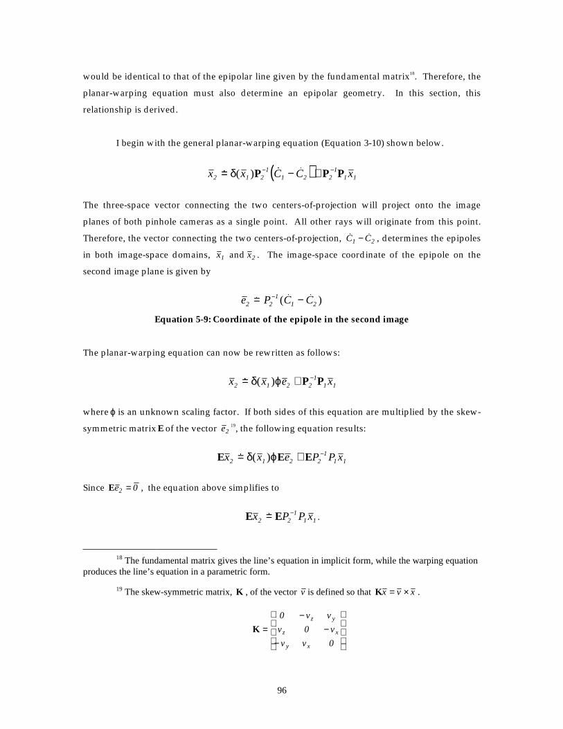
96
would be identical to that of the epipolar line given by the fundamental matrix18. Therefore, the
planar-warping equation must also determine an epipolar geometry. In this section, this
relationship is derived.
I begin with the general planar-warping equation (Equation 3-10) shown below.
( )x x C C x2 1 21
1 2 21
1 1� ( ) � �= − +− −δ P P P
The three-space vector connecting the two centers-of-projection will project onto the image
planes of both pinhole cameras as a single point. All other rays will originate from this point.
Therefore, the vector connecting the two centers-of-projection, � �C C1 2− , determines the epipoles
in both image-space domains, x1 and x2 . The image-space coordinate of the epipole on the
second image plane is given by
e P C C2 21
1 2� ( � � )= −−
Equation 5-9: Coordinate of the epipole in the second image
The planar-warping equation can now be rewritten as follows:
x x e x2 1 2 21
1 1� ( )= + −δ ϕ P P
where ϕ is an unknown scaling factor. If both sides of this equation are multiplied by the skew-
symmetric matrix E of the vector e219, the following equation results:
E E Ex x e P P x2 1 2 21
1 1� ( )= + −δ ϕ
Since Ee2 0= , the equation above simplifies to
E Ex P P x2 21
1 1�= − .
18 The fundamental matrix gives the line’s equation in implicit form, while the warping equation
produces the line’s equation in a parametric form.
19 The skew-symmetric matrix, K , of the vector v is defined so that Kx v x= × .
K =−
−−
0
0
0
v v
v v
v v
z y
z x
y x

97
Now, if both sides are multiplied by x T2 , then
x x x P P xT T2 2 2 2
11 10E E= = − ,
which means that
F EP P21 21
1= − .
Thus, a fundamental matrix can be expressed in terms of the planar-warping equation.
The matrix E is singular and of rank 2, assuring that the product EP P21
1− has the proper form.
As discussed in Chapter 3, the projective map P P21
1− describes a reprojection (i.e., a mapping of
reference-image points to desired-image points in which the center-of-projection does not
change). This mapping is invertible and, therefore, of full rank. The application of the skew-
symmetric matrix, E , removes a dimension from this mapping in the direction of the vector
connecting the two centers-of-projection as illustrated below:
Figure 5-3: Mapping of a unit sphere before and after a skew-symmetric matrix
Thus, given a warping equation, it is straightforward to compute the corresponding
fundamental matrix.
F P P P21 21
1 2 21
1= −− −skew C C( ( � � ))
Equation 5-10: Fundamental matrix in terms of the planar-warping equation
Application of the skew-symmetric matrix of vectorto the subspace of unit-length vectors
*
x
*
x
Before
After
*
x

98
Since it is possible to determine a fundamental matrix from a set of image-space
correspondences between two images, as shown in section 5.1.2, the remainder of this chapter
explores to what extent a warping equation can be determined from a fundamental matrix.
5.2.1 Image Warps Compatible with a Fundamental Matrix
I have already shown, in Equation 5-9, that knowledge of the epipoles is equivalent to
knowing the first term of the planar-warping equation shown below.
x x e x2 1 2 21
1 1� ( )= + −δ ϕ P P
The epipole coordinates are readily determined from a fundamental matrix as follows.
Since all epipolar lines intersect at the epipole, the following relationship must hold:
( )0 21 1 2 1 21 2 1= =F Fx e x e xT T T for all
This can only be satisfied if F21 2 0T e = . This establishes the following homogeneous system of
three equations in three variables20:
f e f e f e
f e f e f e
f e f e f e
11 21 21 22 31 23
12 21 22 22 32 23
13 21 23 22 33 23
0
0
0
+ + =+ + =+ + =
Equation 5-11: Homogeneous system to find the second image’s epipole
In Equation 5-11, and in the next few derivations, I represent the epipole’s coordinate as a
projective point using the following notation: [ ]e e e eT
2 21 22 23= , where the first subscript
indicates the epipole’s image-space and the second indicates the vector element. All other
double-subscripted variables indicate a matrix element.
Since the linear system of Equation 5-11 is homogeneous and the fundamental matrix is
singular, any one of the unknowns can remain unassigned and the remaining two variables can
20 At this point I will drop the subscripts on both the fundamental matrix and the epipole so that
subscripts can be used for identifying the matrix and vector elements. Throughout the remainder of thissection, the epipole’s coordinates can be assumed to be specified in the desired image’s space unless statedotherwise. Likewise, the fundamental matrix can be assumed to map reference image points to epipolarlines on the desired image.
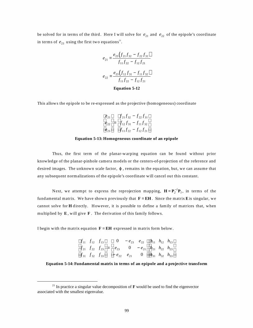
99
be solved for in terms of the third. Here I will solve for e21 and e22 of the epipole’s coordinate
in terms of e23 using the first two equations21.
( )
( )
ee f f f f
f f f f
ee f f f f
f f f f
2123 21 32 22 31
11 22 12 21
2223 12 31 11 32
11 22 12 21
=−
−
=−
−
Equation 5-12
This allows the epipole to be re-expressed as the projective (homogeneous) coordinate
e
e
e
f f f f
f f f f
f f f f
21
22
23
21 32 22 31
12 31 11 32
11 22 12 21
=−−−
Equation 5-13: Homogeneous coordinate of an epipole
Thus, the first term of the planar-warping equation can be found without prior
knowledge of the planar-pinhole camera models or the centers-of-projection of the reference and
desired images. The unknown scale factor, ϕ , remains in the equation, but, we can assume that
any subsequent normalizations of the epipole’s coordinate will cancel out this constant.
Next, we attempt to express the reprojection mapping, H P P= −2
11 , in terms of the
fundamental matrix. We have shown previously that F EH= . Since the matrix E is singular, we
cannot solve for H directly. However, it is possible to define a family of matrices that, when
multiplied by E , will give F . The derivation of this family follows.
I begin with the matrix equation F EH= expressed in matrix form below.
f f f
f f f
f f f
e e
e e
e e
h h h
h h h
h h h
11 12 13
21 22 23
31 32 33
23 22
23 21
22 21
11 12 13
21 22 23
31 32 33
0
0
0
=−
−−
Equation 5-14: Fundamental matrix in terms of an epipole and a projective transform
21 In practice a singular value decomposition of F would be used to find the eigenvector
associated with the smallest eigenvalue.

100
This expression can be expressed as a linear system of 9 equations in 9 unknowns as follows:
f e h e h f e h e h f e h e h
f e h e h f e h e h f e h e h
f e h e h f e h e h f e h e h
11 22 31 23 21 12 22 32 23 22 13 22 33 23 23
21 23 11 21 31 22 23 12 21 32 23 23 13 21 33
31 21 21 22 11 32 21 22 22 12 33 21 23 22 13
= − = − = −= − = − = −= − = − = −
Equation 5-15: Equations for the elements of the fundamental matrix
Six of the nine unknown elements of H can be found in terms of the known values and the three
elements in the last row of H .
e h e h f e h e h f e h e h f
e h e h f e h e h f e h e h f23 21 22 31 11 23 22 22 32 12 23 23 22 33 13
23 11 21 31 21 23 12 21 32 22 23 13 21 33 23
= − = − = −= + = + = +
Equation 5-16: Projective transform’s elements in terms of the fundamental matrix
In matrix form, this expression becomes
[ ]e
f f f
f f f
e
e
e
h h h23
21 22 23
11 12 13
21
22
23
31 32 33
0 0 0
H = − − −
+
,
where h31 , h32 , and h33 are three free parameters that define a family of projective maps which
produce the desired fundamental matrix. If the fundamental matrix is normalized so that
f f f f11 22 12 21 1− = , as in the general seven-parameter form given in Equation 5-5, the following
simplification results:
[ ]H = − − −
+
f f f
f f f
e
e h h hu
v
21 22 23
11 12 13
2
2 31 32 33
0 0 0 1
Equation 5-17: Family of projective transformations compatible with a fundamental matrix
The normalization of the fundamental matrix yields a normalized the epipole coordinate.
This representation of the projective transformations that are compatible with a given
fundamental matrix lends itself to a geometric interpretation. The first term of Equation 5-17
represents the mapping of the desired family of projective transformations onto a plane parallel
to the image plane but passing through the center-of-projection22. The second term represents
22 The projective points on this constitute the projective line at infinity.

101
the components of the projective transform that are lost by such a mapping. Thus, when given
only the fundamental matrix associated with an image pair only the first term and the direction
of the displacement out of the plane of , the projective transformation component of the
associated image warp can be identified. The three parameters, h31 , h32 , and h33represent the
components of projective transformation’s basis vectors that cannot be unambiguously
determined from the fundamental matrix alone. These relationships are illustrated in the
following figure:
Figure 5-4: The projective transformations compatible with a given fundamental matrix
The coordinates of the epipole in the first image can be determined using a derivation
similar to the one shown in Equation 5-11, where the fundamental matrix is replaced with its
transpose. When the fundamental matrix is normalized so that f f f f11 22 12 21 1− = these
expressions simplify to f f e f eu v13 11 1 12 1= − +( ) and f f e f eu v23 21 1 22 1= − +( ) . Substituting
these equalities into the three-parameter family of projective transformations defined in
Equation 5-17 results in the following expression:
[ ]H =− +
− − +
+
f f f e f e
f f f e f e
e
e h h hu v
u v
u
v
21 22 21 1 22 1
11 12 11 1 12 1
2
2 31 32 33
0 0 0 1
( )
Equation 5-18: Family of projective maps in terms of epipoles
Consequently, a fundamental matrix determines the projective mapping component of a
planar-warping equation to within a three-dimensional subspace. This relationship can be
expressed without any explicit knowledge of the intrinsic pinhole-camera parameters, using
h e33
h e32
h e31
Plane parallel to the image plane, butpassing through the center-of-projection

102
only information available from the fundamental matrix. The next section explains another
important special class of projective transformations which will eventually be used to further
constrain the family of projective maps that are compatible with a given fundamental matrix.
5.3 Physical Constraints on Projective Maps
The general projective transformation, H P P= −2
11 , that appears in the warping equation
has eight degrees of freedom. The additional knowledge of an epipolar geometry, as
determined by a fundamental matrix, reduces the available degrees of freedom to three. In this
section, I will introduce additional constraints on the pinhole-camera model which will further
reduce the space of compatible projective transformations. I will also argue that these
additional constraints are reasonable assumptions for a large class of images, including those
acquired by real-world cameras.
5.3.1 Same-Camera Transformations
Consider a canonical planar-pinhole camera that is free to rotate in any direction about
its center-of-projection, which is restricted to the origin (see section 3.4). The image-to-image
mappings that can be represented by such a camera configuration define the family of same-
camera transformations. These transformations have the following algebraic form:
C H U RU= = −samecamera
1
Equation 5-19: Same-camera transformation
The projective transformation, C, determines an image-to-image mapping via the composition
of three transforms. The first is an image-to-ray mapping specified by a canonical pinhole-
camera model, U; the second is a rotation, R, of the camera’s coordinate system; and, the third is
a ray-to-image mapping determined by the canonical pinhole-camera’s inverse, U-1. The same-
camera family of projective mappings is determined by the five intrinsic camera parameters
(defined in Section 4.1.2) of the canonical pinhole-camera model, U, and the three rotational
parameters of R. Three-dimensional rotations, like R, can be parameterized in terms of a unit
vector, r , specifying an axis of rotation and an angle, θ , specifying the amount of rotation.
Restricting the axis of rotation to be of unit-length does not reduce the generality of this
parameterization, and it allows for a minimal specification using only three-parameters.
Same-camera transformations are similarity transforms of rotation matrices, which means
that both C and R will have the same eigenvalues and, hence, the same characteristic

103
polynomials. The characteristic polynomial and the eigenvalues of a general rotation matrix,
such as R, are
λ θ λ θ λ λ λ θλ3 2 21 2 1 2 1 1 2 1 0− + + + − = − − + =( cos ) ( cos ) ( )( cos )
{ }λ θ θ= ±1,cos sini
Equation 5-20: Characteristic polynomial and eigenvalues of a rotation matrix
where θ is the rotation angle about the axis.
The family of matrices equivalent to a given projective transform, C, can be represented
by σC, where σ is a non-zero scalar, since projective transformations scaled by a non-zero scale
factor are equivalent. The same-camera transformations, σC, have the following characteristic
polynomial:
λ σ λ σ λ σ3 2 2
1
33 0− + − =
=∑Trace Minor Determinant( ) ( , , ) ( )C C i i Ci
Equation 5-21: Characteristic polynomial of scaled same-camera warp
The individual terms of Equation 5-20 and Equation 5-21 are equal since the transformations are
similar. The constant terms of the two polynomials can be made equal by selecting an
appropriate scale factor, σ, such that the determinant of σC is one. The expression for this scale
factor is
σ = 13 Determinant( )C
Equation 5-22: Scale factor that makes the determinant of σC equal one
The characteristic polynomial of a rotation has the property that the coefficients of the first and
second degree terms have equal magnitudes and a restricted range. This relationship can be
used to establish constraints on the trace and the sum of the diagonal minors of a same-camera
transformation. By equating the remaining terms in Equation 5-20 and Equation 5-21, subject to
the scaling constraint given in Equation 5-22, the following relationships can be established:

104
Trace
Determinant
Minor
Determinant
( )
( )
( , , )
( )cos
C
C
C
C13
23
1
3
1 2= = +=∑ i ii θ
This yields the following two constraints on a same-camera transformation, C:
Determinant
Minor
Trace( )
( , , )
( )C
C
C=
=∑ i ii 1
3 3
− ≤ ≤1 313
Trace
Determinant
( )
( )
C
C
Equation 5-23: Constraints on a same-camera transformation
These two constraints can be used to verify if a given projective transformation is of the same-
camera class23. Since they depend entirely on the characteristic polynomials of the given
projective transformation, they will be invariant to any transformation of the pinhole-camera
matrix, and are, therefore, independent of the pinhole-camera model U . For example, the
system
C U R U1 11
1 1= −
has the same characteristic polynomial as
C U U R U U2 11
21
1 2 1= − −
Since the upper triangular matrices are a subgroup under matrix composition, the product
U U2 1 can produce a mapping from a given pinhole-camera model to any other. Therefore, the
constraints induced by the characteristic polynomial do not provide any information about the
canonical camera model. Instead they only provide information about the rotation component
of the transformation. For this application, the primary purpose of these constraints is to assure
23 Clearly, there exist matrices outside of this class. For example, consider the class of upper-
triangular projective matrices. In order for U U RU2 11
1= − then U U U R1 2 11− = . Since the class of
upper-triangular matrices is a subgroup of linear transformations under composition the matrix R mustbe a member of that subgroup. But, the only rotation matrices in this subgroup are the identity and theother valid rotations with ± 1 along the diagonal. Thus, upper-triangular matrices are not generally asame camera transformation.

105
that a given transformation will fall within the same-camera subspace of projective
transformation. In the next subsection, I will determine the conditions under which a unique
canonical-pinhole-camera model can be determined from a same-camera transformation.
5.3.2 Determining a Camera Model from a Same-Camera Transformation
Projective transformations that satisfy the same-camera constraints described in the
previous subsection can be used to determine a one-parameter family of pinhole-camera
models. Any one of these pinhole-camera models will be consistent with the given matrix. The
associated rotation matrix can also be derived for any selected camera from this one-parameter
family.
R U CUρ ρ ρ= −1
The one parameter family of pinhole camera models can be determined as follows.
Rewriting C U RU= −1 gives UC RU= . Consider that a rotation of a vector space preserves
both the distances and the angles between vectors24. Therefore, if the columns of U are
considered as vectors, the given expression can be interpreted as follows:
[ ] [ ] [ ]′ ′ ′ = =a b c a b c a b cC R
The following rotational invariants will provide six equations in terms of the nine known
elements from C and the six unknowns from U:
′ ⋅ ′ = ⋅′ ⋅ ′ = ⋅
′ ⋅ ′ = ⋅′ ⋅ ′ = ⋅
′ ⋅ ′ = ⋅′ ⋅ ′ = ⋅
a a a a
a b a b
b b b b
a c a c
c c c c
b c b c
Equation 5-24: Rotational invariants of a same-camera transformation
An equivalent set of equations can be found algebraically by multiplying UC RU= by
its transpose, C U U RT T T T= , which gives C U UC U UT T T= . The symmetric matrix S = UTU
has the six invariant quantities as its elements.
24 The so-called Euclidean metrics.

106
C
a a a b a c
a b b b b c
a c b c c c
C
a a a b a c
a b b b b c
a c b c c c
T
⋅ ⋅ ⋅⋅ ⋅ ⋅⋅ ⋅ ⋅
=⋅ ⋅ ⋅⋅ ⋅ ⋅⋅ ⋅ ⋅
Equation 5-25: Rotational invariants expressed as a matrix product
Equating the matrices on an element-by-element basis yields six unique equations that
are identical to those derived earlier using the geometric argument. In the case where the same-
camera transformation is known, this system of equations will be linear in the six unknown
elements of the symmetric matrix S. The resulting homogenous system of linear equations is
shown below.
c c c c c c c c c
c c c c c c c c c c c c c c c c c c
c c c c c c c c c c c c c c c c c c
c c c c c c c c c
c c c c c c c
112
11 21 11 31 212
21 31 312
11 12 11 22 12 21 11 32 12 31 21 22 21 32 22 31 31 32
11 13 11 23 13 21 11 33 13 31 21 23 21 33 23 31 31 33
122
12 22 12 32 222
22 32 322
12 13 12 23 13 22 12
1 2 2 2
1
1
2 2 1 2
−− − + −
− + − −−
+ c c c c c c c c c c c
c c c c c c c c c
a a
a b
a c
b b
b c
c c33 13 32 22 23 22 33 23 32 32 33
132
13 23 13 33 232
23 33 332
1
2 2 2 1
0
0
0
0
0
0
+ − −−
⋅⋅⋅⋅⋅⋅
=
Equation 5-26: Homogenous linear system determined by C
This linear system only has a rank of 4, and, therefore, has a two-parameter family of
solutions25. One of these parameters can be established by fixing any one of the three vector
lengths to 1. Since the pinhole-camera model, C, is only defined to within a scale factor,
choosing one vector’s length does not affect the solution.
The constraints, a a⋅ = 1 and a b s⋅ = , provide a convenient parameterization that also
has a useful geometric interpretation. It also results in a pinhole-camera model in the
normalized canonical form of Equation 4-6. The angle a b⋅ is a measure of the skew between the
image-space basis vectors, discussed in Chapter 4. In most real-world image-acquisition
systems, this skew factor is nearly 0 because typical solid-state sensors, such as charge-coupled
devices, are manufactured to precise standards in which the orthogonality of the two-
dimensional array of photosites is nearly guaranteed. Thus, we can limit our consideration of
viable same-camera transformations to those where the s component of the associated pinhole
camera is nearly 0. Since s is physically linked to the inner products of two vectors (one
25 The lower-right 4 × 4 submatrix will, in general, have a non-zero determinant. Any larger
submatrix will always have a determinant of zero, when the determinant and trace constraints of thesame-camera transform are considered. Thus the linear system has a rank of four.

107
constrained to a unit length and the other of a computed length), our interpretation of s can
easily be mapped to an angle, and, therefore, made independent of an external scale. This is
important because it allows us to consider the smallness of s within a fixed context. In general,
we also expect b b a a r⋅ ⋅ ≈ 2 , since the ratio of the lengths is indicative of the aspect ratio, r, of
the sampling grid, and this value is usually known in most real imaging systems.
Figure 5-5: The skew and aspect ratio properties of a planar-pinhole camera
A canonical planar-pinhole camera model can be determined by substituting the
elements of the solution vector from Equation 5-26 into the expression given in Equation 4-5 and
choosing the positive-valued square roots for the diagonal elements. When the parmeterization,
a a⋅ = 1 and a b s⋅ = , is chosen for the homogenous linear system, the following planar-pinhole
camera model results:
PC =
⋅
⋅ − = ⋅ − ⋅
⋅ −⋅ − ⋅ −
1
0
0 0 2 2
s a c
b b sb c s a c
b b s
c c a c
( )( ) ( )
( )
( ) ( )
χ
χ
Equation 5-27: Planar-pinhole camera model of a same-camera transform
Ordinarily, we would expect that s≈ 0 and the term ( )b b s⋅ − to be approximately the
height-to-width aspect ratio of the sampling grid. Under typical conditions, we would also
expect a c⋅ < 0 and χ < 0 if the image-space origin is considered to be the upper-left corner of
the image.
A skewed viewing plane withnon-orthogonal spanning vectors
A viewing plane with a non-square sampling grid and
aspect ratio
s≠ 0 b ba a
⋅⋅ ≠ 1

108
5.3.3 Closed-form solutions for the intrinsic camera-parameters
Given a specific instance of a projective transformation, which satisfies the same-camera
constraints of Equation 5-23, the homogeneous linear system of Equation 5-26 can be solved
using either a global optimization method or a singular-value decomposition if sufficient
constraints are imposed such that there is a unique solution. Hartley has shown that when
given three or more images taken from a common center-of-projection a solution can be found
using a global optimization method, with the exception of a few degenerate the camera
configurations [Hartley94]. By using multiple images he was able to avoid imposing any
external constraints. However, the non-linear optimization method that he employed required
an initial estimate of the intrinsic parameters that are being solved for.
Here, I will propose an alternate approach to this problem that provides a closed-form
solution. Closed-form solutions are useful because they can be computed without an initial
estimate of the final solution, they require a constant time to compute, and they can be further
analyzed. Since the solution-space of intrinsic-camera parameters that are consistent with a
same-camera transformation are a two-dimensional subspace within the six-dimensional space
of upper-diagonal matrices, additional constraints are required to guarantee that the solution is
unique. I will assume a unit-length spanning vector and zero-skew constraint on the solution
space, which is a reasonable assumption for most camera configurations, as discussed
previously. When these constraints are substituted into Equation 5-25 the following rotational
invariants result:
c c c
c c c
c c c
a c
b b b c
a c b c c c
c c c
c c c
c c c
a c
b b b c
a c b c c c
T11 12 13
21 22 23
31 32 33
11 12 13
21 22 23
31 32 33
1 0
0
1 0
0
⋅⋅ ⋅
⋅ ⋅ ⋅
=⋅
⋅ ⋅⋅ ⋅ ⋅
Equation 5-28: Constrained rotational-invariant matrix
In order to simplify subsequent derivations I will introduce the following elements of
C’s adjoint matrix as constants:

109
Z =− − −− − −− − −
c c c c c c c c c c c c
c c c c c c c c c c c c
c c c c c c c c c c c c
22 33 23 32 13 32 12 33 12 23 13 22
23 31 21 33 11 33 13 31 13 21 11 23
21 32 22 31 12 31 11 32 11 22 12 21
Note that C ’s adjoint matrix, Z , is also C ’s inverse since C has a determinant of 1. In
addition, the trace of this adjoint matrix is equivalent to the sum of C ’s diagonal minors. Thus,
by the same camera constraints, Trace Trace( ) ( )C Z= .
Arbitrary equations in the remaining four unknowns of the symmetric matrix can be
generated by multiplying Equation 5-28 by any column vector on the right and any row vector
on the left, u v u vT T TC SC S= . Some care must be exercised to assure that the resulting
equations are linearly independent. Generally three choices of vectors v u1 1= , v u2 2= , and
v u3 3= , such that [ ]det v v v1 2 3 0≠ (i.e., the three vectors are not collinear) along with a fourth
vector, v u4 4≠ , will suffice. Furthermore, if the vectors are selected appropriately, very simple
expressions can result. For example, the vector [ ]u v c cT= = −32 31 0 gives the following
expression:
b bc z
z cGeneral⋅ = −
−322
322
312
312
Equation 5-29: Closed-form solution for the quantity b b⋅ in the general case
This equation will hold unless either or both of the c31or c32 elements of C are zero.
These special cases, which include the affine subset of same-camera transformations, are treated
separately in Appendix B. A similar application of the vectors [ ]u vT= = 0 0 1 in conjunction
with various substitutions will give the following expression for c c⋅ in terms of b b⋅ :
c cb b c c z c c c c c z c c z c c c c c z
c c c c c c cGeneral⋅ =
⋅ − + − + − + −+ + −
( )( ( )) ( ( ))
( )13 32 21
223 31 23 32 33
2112
31 23 122
32 13 13 31 332
222
31 32 13 31 23 32 332 1
Equation 5-30: Closed-form solution for the quantity c c⋅ in the general case
Using a similar approach the following expressions for the two remaining components of S can
be found:

110
a cc c c b b z c z
c c
b cc c c b b c z z
c c
General
General
⋅ = ⋅ − ⋅ + −
⋅ = ⋅ + ⋅ − −
( ) ( )
( ) ( )( )
312
212
332
222
31 33
322
332
112
122
32 33
2
2
Equation 5-31: Closed-form solution for the quantities a c⋅ and b c⋅ in the general case
These four quantities can be substituted into Equation 5-27 to compute the canonical
pinhole camera model. Therefore, a closed-form solution for the planar pinhole-camera model
can be determined for any projective mapping satisfying the constraints of a same-camera
transformation given the prior knowledge that the imager has an orthogonal sampling grid.
This result can be used to determine the calibration any of such a camera given only two images
taken from a common center of projection. The only limitation of the given equations is that
both of the c31or c32 elements of C are required to be nonzero. However, equivalent solutions
for these four unknowns can be derived for all these cases with the notable exception of the
affine case in which both c31 and c32 are zero. Only three of these four parameters can be
found in the affine transformation case; a detailed discussion of this case is given in Appendix B.
Consider the following example. Given the following rotation matrix and pinhole-
camera model, which represents a 512 × 512 image with a 45° horizontal field-of-view
symmetric frustum:
[ ]R P( , )
. . .
. . .
. . .
. -37
67
27
T π9
0950769 0119873 0 285775
0 0755662 0984000 0161349
0300544 0131810 0944615
1 0 256
0 098 256
0 0 618
≈−
− −
=−−
a same-camera transformation and its inverse can be computed as
C Z=−
−− −
=−
− −
0826271 0170985 251570
0 0499298 0 929398 118505
0 000486318 0 000209020 112371
106914 0139555 254 072
0 00152468 105083 110 479
0 000462419 0 000255861 0 759398
. . .
. . .
. . .
. . .
. . .
. . .
The rotationally invariant quantities of the same camera transformation can be determined
using the closed-form equations as follows (six-significant digits were maintained throughout all
calculations):

111
b b
c c
a c
b c
⋅ ≈⋅ ≈ ×
⋅ ≈ −⋅ ≈ −
0 960382
513098 10
256 027
250 905
5
.
.
.
.
Finally, the pinhole-camera’s intrinsic parameters can be determined from Equation 5-27.
~.
. .
.
P =−−
1 0 256 027
0 0 979990 256 027
0 0 618 059
This technique could be used as a calibration process for computing intrinsic-camera
parameters based solely on image observations. The camera, whose sampling grid is assumed
to be orthogonal, must first be placed on a tripod or rotational stage and adjusted so that its
panning motion is about the camera’s center-of-projection. This can be accomplished by
translating the camera in the plane perpendicular to the rotational axis until there is no apparent
change in parallax. Any pair of images taken with this configuration are related by a same-
camera transformation. The actual transformation can be determined using a well-known linear
method described by both [Heckbert89] and [Wolberg90] which requires the identification of a
minimum of four corresponding points in each image. Typically, many more points would be
used in conjunction with a least-squares solution method. Once the transform was found it
should be verified that it satisfies the same-camera constraints of Equation 5-23. If these
constraints are not satisfied, the matrix must somehow be minimally perturbed such that it has a
valid characteristic polynomial. Once this is completed, the closed-form solution method
demonstrated in the previous examples can be used to find the camera’s intrinsic parameters.
In addition, the extrinsic parameters representing the rotation between the two images can be
determined as follows:
R PCP= −1
Equation 5-32: The rotation between the camera models of a same-camera transform
5.4 Deriving a Planar Pinhole-Camera Model from Images
Next, I consider the problem of establishing a warping equation for a reference image
whose extrinsic and intrinsic pinhole-camera parameters are unknown. In order to establish the
generalized-disparity values for the reference image, at least one other image is required in
order to determine correspondences. I will require that both the reference image and the second

112
image used for correspondence be acquired using the same camera. In such a case, the
relationship between the second image’s planar pinhole-camera model to the pinhole model of
the reference image is given by P R P2 2 1= , and the corresponding warping equation has the
following form:
x x C C x2 1 11
21
1 2 11
21
1= − +− − − −δ( ) ( � � )P R P R P
Equation 5-33: Planar warps resulting from the same camera
As one would expect, the matrix product in the second term of Equation 5-33 is a same-camera
transformation.
Once eight or more corresponding image-space points are identified in the two images,
a fundamental matrix can be determined using the methods outlined in subsection 5.1.2. This
fundamental matrix establishes the epipolar geometry between the two images. The
determinant of the upper-left 2 × 2 submatrix of this fundamental matrix can then be tested for
generality. If this determinant is nonzero (both epipoles are finite), the fundamental matrix can
then be normalized by scaling it by the reciprocal of the determinant’s square-root. In this
typical situation a three-parameter family of projective transformations compatible with the
computed fundamental matrix can be identified using Equation 5-18. We can further limit this
three-parameter space of projective transforms to those that also satisfy the same-camera
transform constraints derived in section 5.3.1. Equations for the scalar-matrix quantities used to
determine these constraints for this three-parameter family of projective transforms are given in
the following subsection.
5.4.1 Scalar matrix quantities of transforms with known epipolar geometries
In this subsection I define the matrix relationships necessary to determine if a projective
transformation that is compatible with a given fundamental matrix is also in the same-camera
family. I will refer to an instance of a projective transformation that is compatible with the given
fundamental matrix F, as specified in Equation 5-18, as σH F . Recall that the fundamental
matrix of Equation 5-18 has been normalized so that it is of the form given in Equation 5-5. The
non-zero scale factor, σ, is included because all such projective transformations are equivalent.
The same-camera transformation constraints, derived in Equation 5-23, are specified in terms of
three scalar matrix quantities: the determinant, the trace, and the sum of the diagonal minors.

113
The determinant of σH F is
Determinant( ) ( ( ) ( ) )σ σH F = − + − +331 12 23 22 13 32 21 13 11 23 33h f f f f h f f f f h
The coefficients of h31 , h32 , and h33 are the coordinates of the null-space vector in the
fundamental matrix’s transpose. This can be seen by comparing the coefficients to Equation 5-
13. Therefore, these coordinates identify the epipole of the reference image (i.e., the projection
of the second image’s center-of-projection in the reference image). I will refer to the screen-
space coordinate of the reference image’s epipole as [ ]e e eu vT
1 1 1 1= 26. Substituting the
epipole’s coordinates into the equation above gives
Determinant( ) ( )σ σH F = + +331 1 32 1 33h e h e hu v .
Equation 5-34: Determinant of a transform compatible with a given fundamental matrix
The trace of σH F is
Trace( ) ( )σ σH F = + + + −h e h e h f fu v31 2 32 2 33 21 12
Equation 5-35: Trace of a transform compatible with a given fundamental matrix
The sum of the diagonal minors of σH F is
Minor( , , ) ( ( ) ( ) ( ) )σ σH F i i h f e f e f h f e f e f h f fi
u v u v=∑ = − + + + + + + − +
1
32
31 12 2 22 2 23 32 11 2 21 2 13 33 21 12 1
The expression for e2 ’s coordinates given in Equation 5-11 can be used to simplify this
expression. Note that in the assumed normalization, the term e f f f f23 11 22 12 21 1= − = . This
gives the expressions f e f e fu v11 2 21 2 31 0+ + = and f e f e fu v12 2 22 2 32 0+ + = . Rearranging and
substituting these terms into the expression for the sum of the diagonal minors shown above
gives
26 The coordinates of the epipole in the first image, e1, are generally different from the
coordinates of the epipole in the second image, e2 . Even when they have the same coordinate values,
they are still defined in different screen spaces.

114
Minor( , , ) ( ( ) ( ) ( ) )σ σH F i i h f f h f f h f fi=∑ = − + − + − +
1
32
31 32 23 32 13 31 33 21 12 1
I will introduce the following notation in order to simplify later expressions:
~m
m
m
m
f f
f f
f f
=
=−−−
1
2
3
32 23
13 31
21 12
Equation 5-36: Vector of minor coefficients
This substitution gives the following simplified expression:
Minor( , , ) ( )σ σH F i i h m h m h mi =∑ = + + +
1
32
31 1 32 2 33 3 1
Equation 5-37: Sum of the diagonal minors of compatible transforms
5.4.2 Finding a Camera Solution
In order for a given transformation to be a member of the same-camera class, the scale
factor of the transform, σ, must be selected so that its determinant is equal to one. This
constraint gives the following expression:
h e h e hu v31 1 32 1 33 3
1+ + =σ
Equation 5-38: Unit-determinant constraint
The second constraint on a same-camera transformation is that its trace must equal the
sum of its diagonal minors. The equivalence of the trace and the sum of the diagonal minors
can be expressed by subtracting Equation 5-37 from Equation 5-35. The following equation
results:
σ σ σ σ σ( ( ) ( ) ( ) ( ))h e m h e m h m mu v31 2 1 32 2 2 33 3 31 0− + − + − − − =
If σ is zero, the resulting transformation cannot have a determinant of one as required by
Equation 5-38. Thus, σ is non-zero and it can, therefore, be factored out giving
h e m h e m h m mu v31 2 1 32 2 2 33 3 31( ) ( ) ( ) ( )− + − + − = −σ σ σ σ
Equation 5-39: Trace-equals-sum-of-minors constraint

115
Both Equation 5-38 and Equation 5-39 are of degree one in terms of h31 , h32 , and h33 .
Therefore, for any fixed value of σ the locus of points in the parameter space which satisfy the
unit-determinant constraint is a plane. Likewise, the locus of parameter-space points that satisfy
the trace-equals-the-sum-of-minors constraint is also a plane. The intersection of these two
planes represents the set of transformations where both constraints are satisfied. Generally, the
intersection of two planes will be a line. As the parameter σ is varied, a family of lines is swept
out in the parameter space. These lines define a two-dimensional subspace of projective
transformations that are compatible with the given fundamental matrix and are potentially
same-camera transformations. An example of this two-parameter surface is illustrated below.
Figure 5-6: Surface of potentially compatible projective transformations
Next, I will reformulate the surface description in terms of two parameters to facilitate
searching for a valid camera model. The first parameter will be the scale factor σ . The second
is the trace of the projective transform prior to scaling, which will be represented by the symbol
τ.
τ = + + +h e h e h mu v31 2 32 2 33 3
Equation 5-40: The trace of the desired transform prior to scaling
The three parameters h31 , h32 , and h33 , which define the subspace of projective
transformations compatible with a given fundamental matrix, can be expressed in terms of
σ and τ as follows:
h33
h31
h32
Planar loci of unitdeterminants
Loci where traceequals the sum of
the diagonalminors

116
hm e m m e e e e e m m
m e e m e e m e e e e
he e
h e e m
e e
h h e h e
v v v v v v
v v u u u v v u
v v
u u
v v
u
31
32 1 3 3 1 2
21 2 2 3 2
31 1 2 2 1 2 3 1 2 1 2
32 31 2
31 1 2 3
1 2
33 3 31 1 32
1
1
= − − − − + − + −− − − + −
=−
− − − +−
= − −
σ τ σ τσ
στ
σ
(( )( ) ( )) ( )
( ( ) ( ) ( ))
( )
( )
( )
1v
Equation 5-41: Expressions for h31, h32, and h33 in terms of σ and τ
The parameterization of the compatible same-camera surface given in Equation 5-41 is suitable
for all cases except when the epipoles of both images have the same coordinate. This special
case is discussed further in Appendix C.
The final identification of the projective transformation, which is both a same-camera
transformation and is compatible with the given fundamental matrix, requires that three
additional relational constraints be satisfied. These constraints are listed below.
1 1 3
2 0
3 0
)
)
)
− ≤ ≤⋅ ≥⋅ ≥
στb b
r r
Equation 5-42: Three relational constraints on a same-camera transformation
The last two relationships can be tested using Equation 5-29 and Equation 5-30 on the
parametric surface described by Equation 5-41. The elements of the matrices C and Z in terms
of h31 , h32 , and h33 , are given below. It is assumed that these terms result from Equation 5-41.
C
Z
F
u u u
v v v
F
u
v
h e f h e f h e f
h e f h e f h e f
h h hh f h f h f h f h f h f e
h f h f h f h f h f h f e
h f h f h f h
=+ + +− − −
=− − − +− − − +− −
σ
σ
31 2 21 32 2 22 33 2 23
31 2 11 32 2 12 33 2 13
31 32 33
232 13 33 12 32 23 33 22 32 33 33 32 1
33 11 31 13 33 21 31 23 33 31 31 33 1
31 12 32 11 31 22 32 21 31 32 32 311f h f h f− +
Equation 5-43: Same-camera transform and adjoint compatible with F
The matrix elements from Equation 5-43 allows Equation 5-29 and Equation 5-30 to be
evaluated for arbitrary points on the surface of potentially compatible transforms. Using these
results, the second two relationships of Equation 5-42 can be tested. Figure 5-8 illustrates the
subspace of potentially compatible transforms satisfying the conditions of Equation 5-42.

117
Figure 5-7: The solution space of compatible same-camera transformations
Figure 5-8 shows a solution space for a particular same-camera model. The scale-factor
parameter, σ , is shown in a range of -2 to 2. The horizontal axis represents the product of the
two parameters, στ , in the range from -2 to 4. In this parameter space the first relational
constraint of Equation 5-42 defines the vertical band the range from − ≤ ≤ −1 3στ . The rotation
angle of the same-camera corresponding to the στ value is shown across the top of the figure.
The darkened curve indicates regions of the parameter space where one or both of the two
remaining relational constraints of Equation 5-42 are satisfied. Only within the black region are
all three conditions satisfied.
The fundamental matrix used to illustrate the solution-space in Figure 5-8 was
determined by 28 corresponding points selected from two images with resolutions of 768× 512
pixels. This fundamental matrix was found using the methods described in section 5.1.2. The
error in a fundamental matrix can be quantified by computing the average distance of all
identified points from the line produced by their corresponding point in the other image. In this
example, this average error is 0.3894 of a pixel. The values of this matrix and its associated
epipoles, shown to six significant figures, are
στ
σ
-1 0 321
-1
0
1
0°90°180° 60°120°

118
F21 1 2
0 0836038 0 981640 305318
103385 0177880 207391
472 261 363335 37892 4
149 273
298315
1
459 641
493967
1
=− − −
− −
=−−
=−−
. . .
. . .
. . .
.
.
.
.e e
Equation 5-44: Fundamental matrix used in Figure 5-8
The valid same-camera solutions are restricted to a compact region of the solutions
space. While it might be possible to derive a closed-form solution for a camera model within
this enclosed region, the high-degree of the polynomial expressions involved would likely lead
to numerical instabilities in computing such a solution. Furthermore, it is well known that such
high-order rational systems are extremely sensitive to any noise in the input. Instead of seeking
a closed-form solution, a global-optimization method can be used to identify a specific camera
model within this region. This requires the selection of an appropriate penalty function based
on a reasonable set of assumptions concerning the camera model. I have employed the
following penalty function for this purpose:
E b b e e ec ca c w
w
b c h
h( , ) ( )( / ) ( / )
σ τ κ α κ κα
α= ⋅ − + + − + −
− ⋅− ⋅ + − ⋅ +
12 2
2 3
2 2
1 1
2 2
Equation 5-45: Error function used in the global optimization
The first term of the penalty function biases the solution toward the estimated aspect-ratio, α ,
of the image sampling grid (in the absence of other information, a value of α = 1 is usually safe
unless there is noticeable aspect-ratio distortions in the image). The second term drives the
solution away from negative values of c c⋅ , and the third term of the error function, where w
and h represent the image’s width and height in pixels, causes the solution to prefer nearly
symmetric viewing frustums. The weighting factors κ1 , κ 2 , and κ 3 control the relative
importance of each penalty term. Values of κ1 1= , κ 2 1= , and κ 3 01= . have given reasonable
results, and variations in these weighting factors have very little influence on the final camera
model.
A Levenberg-Marquardt global optimization method was used to solve for the final
camera model [Press88]. This optimization method generally converges rapidly if the initial
estimates of σ and τ are near the actual solution. Such an initial estimate can usually be made
when the solution space is contained in a compact region like that shown in Figure 5.827.
27 While the possibility of multiple solutions within this region exists, the variations in the
resulting camera models are minimal. However, it has been observed that this variation increases

119
The final camera model derived from the fundamental matrix of Equation 5-44 is
P P1 2
1 0 381504
0 0999951 191141
0 0 643787
= =−−
.
. .
.
Equation 5-46: Estimated camera model
where σ = 114196. and τ = 259207. . This model can be compared to a simple pinhole-camera
model using manufacturer’s lens specifications. Both images were taken using a 28mm focal-
length lens and captured on a 36mm by 24mm image plane focused at a distance of
approximately 1.5m. The image plane dimensions and effective focal length28 must be scaled by768
36pixels
mm to be in the same units as Equation 5-46. The resulting simple pinhole-camera model
using the manufacturer’s specification is
PSimple =−−
1 0 384
0 1 256
0 0 608 696.
Equation 5-47: Simple pinhole-camera model using manufacturer’s specs
5.5 An Example
The following example illustrates the entire process of building an image-based model
without a priori knowledge of the camera calibration. The images shown below were taken
with the same camera using a fixed focal-length lens with constant shutter and aperture settings.
A total of 48 corresponding points are identified in each image, and they are shown as crosses.
The original contrast of the image has been reduced so that the annotations are visible.
dramatically as the rotation angle approaches 0. Appendices C and D address these numerically difficultsituations.
28 The effective focal length is computed using the thin lens law 1 1 1f f deffective l object
= − , where fl is
the focal length and deffective is the distance to the object in focus.

120
Figure 5-8:
The fundamental matrix was then computed using the linear method described by
[Hartley92]. Next a Levenberg-Marquardt nonlinear optimization similar to the one described
by [Luong93b] was used to minimize the error in the fundamental matrix. The 7-parameter
model given in Equation 5-5 was used to describe the fundamental matrix in the optimization
process, and the linear-solution was used as an initial guess. The resulting epipolar lines are
shown below superimposed over the image and the given correspondences.
Figure 5-9
The image was then rectified, using a method similar to the one described by [Seitz96],
by transforming the epipole in each image to [ , , ]0 1 0 T using a three-dimensional rotation and an
affine transformation. In this configuration, the epipolar lines are aligned with the vertical
columns of the image. A correlation-based method using a 5 × 5 sliding window was then used
to compute the disparity value at each pixel in the right image, which will be the reference. The

121
inverse of the rectification transform was then applied to the right image to provide the final
disparity values. These generalized-disparity values are shown below.
Figure 5-10
The fundamental matrix was then used to estimate a same-camera model. The results of
several image warps based on this model are shown below.
Figure 5-11

122
5.6 Discussion
This chapter has addressed the problem of determining a planar image-warping
equation when the center-of-projection and the pinhole-camera model of the reference image are
unavailable. This allows for the generation of image-based computer graphics with no external
information beyond a reference image and a second image from the same camera for
establishing correspondences. Alternatively, these results might be used to find the calibration
of a pinhole-camera model based on the epipolar geometry determined from image
observations29.
Maybank [Maybank92], Faugeras [Faugeras92a], and Luong [Luong93a] have described
a similar method for determining a pinhole-camera model from an epipolar geometry. Their
method requires three camera displacements (i.e., four images with associated
correspondences) and is able to determine all five intrinsic camera parameters without any
assumptions. [Maybank92] provides a formal proof for the uniqueness of their solution.
Maybank’s, Faugeras’, and Luong’s self-calibration method establishes two conic
expressions from each epipolar geometry, whereas the approach described here derives four
equations from a rank-deficient 6 × 6 system describing the rotational geometric invariants
(Equation 5-26). In such a system, four of the unknowns can be solved for in terms of the
remaining two. The values of these remaining two unknowns can be established under two
assumptions. The first assumption, limiting the length of one of the spanning vectors, is
equivalent to a scaling of the pinhole-camera model and therefore does not limit the solution
space. The second assumption limits the solution space to pinhole-cameras with orthogonal
sampling grids. This is reasonable for most real-world cameras. Both self-calibration methods
suffer from numerical sensitivities.
Hartley [Hartley94] has described another self-calibration method based on a rotating
camera. Since all of the images in his method are required to have the same center-of-projection,
no epipolar geometry is defined. His approach is similar to determining a camera model from a
same-camera transformation as described in section 5.3.2. Hartley’s method determines all 5
pinhole-camera parameters and uses a global optimization to find the desired camera model.
29 In the approach described, only 4 of the 5 intrinsic camera parameters (the fifth skew
parameter is assumed to be zero) and 5 of the 6 extrinsic parameters (all three rotation parameters and avector in the translation direction) can be found.

123
The same-camera method that I described can only determine four parameters within a
restricted subspace. However, it does provide a closed-form solution for that case.
There are still several open issues concerning the self-calibration method that I have put
forth. For practical use, the numerical stability and special-case handling of this solution
method are important concerns that need to be addressed. A complete analysis of the problem’s
numerical sensitivity, along with the development of a computation strategy for maintaining the
greatest possible accuracy in the solution, would be a valuable addition to this work.
Furthermore, an interesting open question is whether the described approach leads to a unique
solution in all cases.
Algebraic curve theory might provide an answer to the uniqueness question. By
determining the rank of each constraint curve, it is possible to determine the number of times
that a general line will intersect the curve. An examination of the degree and rank of the
algebraic expression’s denominator allows the number of unique components to be determined.
Careful analysis of the curve components that are intersected by vertical lines through the
region of the solution space between − ≤ ≤1 3σt might provide an upper-bound on the number
of regions in which the remaining two relationships of Equation 5-42 can be simultaneously
satisfied.
Alternatively, a visualization of the solution space of potential same-camera transforms
that are compatible with a given epipolar geometry can be used to establish an initial guess for a
global optimization method. In this chapter I have also provided a suitable error function for
use in this global optimization process.

124
&KDSWHU �
COMPUTING VISIBILITY WITHOUT DEPTH
Recall that in Chapter 3 an algorithm was presented for computing a correct visibility
solution for a warped image. This algorithm establishes an ordering for the warping that back-
to-front. In this chapter I will prove the correctness of this visibility algorithm. I will adopt a
spherical pinhole-camera model instead of the planar pinhole-camera model used in the original
algorithm. Because a spherical pinhole-camera model is panoramic, as described in Chapter 4,
all the rays originating from its center-of-projection have a unique description. Using a spherical
model has two benefits. First, there will always be an image of the desired center-of-projection
on a spherical viewing surface of the reference image; this halves the number of enumeration
cases. Second, since the projected image of the desired center-of-projection will always fall
within the parameter domain, the nine cases described in section 3.5.1 all reduce into one case.
Once the algorithm is proven correct for the spherical case, it is straightforward to extend it to
the planar model.
In this chapter I provide a formal proof for the visibility algorithm's correctness in the
case of a spherical viewing plane. I then extend this result to planar-viewing surfaces. Finally, I
present a summary of how to extend the algorithm to any other viewing surface. In the
following chapter I will return to more general discussions of the image-based approach.
6.1 Definitions
A perspective-projected image is defined by a central point and a single-valued range
function specified over a bundle of rays emanating from that point. Coordinates are assigned to
rays using a parameter space defined on some viewing surface. This central point of the
perspective-projected image is its center-of-projection. Any perspective-projected surface has a
dual representation - the mapping of the ray bundle onto a spherical viewing plane having the
same center-of-projection. Within such a framework, all rays have a unique coordinate.

125
In this derivation I will consider a set of spherical coordinate frames, { }S S Sn1, , ,2 � ,
embedded within a global Cartesian coordinate system, W . An example is shown in the
following figure:
Figure 6-1: Spherical coordinate frames embedded in a Cartesian coordinate system
The origin of a spherical frame represents a center-of-projection with a unit sphere as a viewing
surface.
This analysis assumes the existence of scene points somewhere within the global
coordinate frame, W . For each scene point there exists a mapping from the global coordinate
frame to the coordinate frame of any spherical domain.
This mapping of points from W to Si is not necessarily one-to-one. I will consider a
particular subset of this mapping that assigns coordinates to only those points closest to the
frame’s center-of-projection along each ray. This particular mapping is called an occlusion-
compatible mapping, and it is consistent with a proper visibility solution for opaque surfaces.
Chapters 3 and 4 described image warping equations that mapped the visible points
seen from one center-of-projection to their correct coordinate in any other projective image.
However, these two-dimensional image-warping functions might map several points from the
original image’s domain to a single point in the final image. Such a point in the final image will
be referred to as a multiplicity of the mapping. The specific claim of this proof is that an
x y
z
S1 S2

126
occlusion- compatible mapping can also be established independent of the scene points’
distances from either the original or final centers-of-projection.
6.2 Proof
In this discussion the initial projective image is assumed to be the Si frame, and the
desired image's frame is Sj . In general all possible reprojections of a point, x , that fall along a
given ray, ( )θ φx x, , of Si are constrained to lie within a plane. This plane is defined by the line
segment, l, connecting the initial and desired centers-of-projection and the ray itself. There are
two exceptions to this. On a spherical viewing surface there exists one ray in the direction of the
line segment connecting the two centers-of-projection. This ray, ( )θ φ+ +, , which is called the
positive epipole, is the virtual image of the desired center-of-projection on the original surface.
The ray in the opposite direction is called the negative epipole, ( )θ φ− −, . It corresponds to the
vanishing point for all rays originating from Sj in the direction of Sj when projected onto Sj ’s
viewing surface. Points along either of these epipolar rays are constrained to lie on the line that
has l as a segment. This line is also common to all the planes associated with a ray, as
discussed previously. These constraint planes are called epipolar planes. The projections of these
epipolar planes onto the viewing surface lie along longitudinal lines of a sphere having the
epipoles as poles. This relationship is shown in the following figure:
Figure 6-2: An epipolar plane defined by a ray and two centers-of-projection
Next, consider an isolated multiplicity on the projective mapping from Si to Sj , as
shown in the following figure:
( , )θ φx x
( , )θ φ+ +
SphericalFrame Sj
SphericalFrame Si

127
Figure 6-3: A multiplicity induced by translation of coordinate frames
Theorem 1. The points of a multiplicity and the centers of Si and Sj are coplanar,except when the multiplicity lies along an epipole.
Proof: The points of the multiplicity are collinear with the origin of Sj since they share
the same coordinates. A second line segment connects the frame origins, Si and Sj . In
general these lines are distinct and, since they share a common point, they must be
coplanar. If the points of the multiplicity happen to fall along the line containing the
segment connecting Si and Sj , then no unique plane is determined.
It follows from the definition that the plane of a multiplicity is also an epipolar plane.
This plane is common to all of those rays in the original image whose points map onto the
multiplicity. Thus, from Theorem 1, we can conclude that all of the multiplicities that are
introduced by projective mappings occur entirely within epipolar planes.
Having established the importance of epipolar planes, it is now only necessary to
consider points within a particular epipolar plane throughout the remainder of the proof.
Assume that a Euclidean or rigid-body transformation is applied to the global coordinate frame,
W , that simultaneously aligns the epipolar ray with the x-axis and the epipolar plane of interest
with the x-y plane. Then consider a uniform scaling of the global coordinates such that the
distance between the centers-of-projection is 1. This transformation can also be thought of as a
re-parameterization of three-dimensional space. This situation is shown in the following figure:

128
Figure 6-4: A multiplicity illustrated in an epipolar plane
Theorem 2. If cos cosθ θ1 2> and 0 1 2< <θ θ α π, , , then a < b.
Proof: The length of sides a and b can be found in terms of the angles θ θ1 2, , and αusing the law of sines as follows:
( ) ( )a b
sin sin sin sinθ α θ θ α θ1 1 2 2
1 1=−
=−
Thus,
( ) ( )a b=−
=−
sin
sin
sin
sin
θα θ
θα θ
1
1
2
2
and
a b=−
=−
sin
sin cos cos sin
sin
sin cos cos sin
θα θ α θ
θα θ α θ
1
1 1
2
2 2
a b=−
=−
1 1
1 2sin cot cos sin cot cosα θ α α θ α
The denominators in the expressions of a and b must be strictly positive, since the
lengths of a and b are positive over the range of angles defined. The ratio of a to b
can be expressed as
a
b=
−−
sin cot cos
sin cot cos
α θ αα θ α
2
1
Si Sj
b
a
αθ1
θ2
p2
p1
α−θ2
α−θ1
1

129
The given relationship
cos cosθ θ1 2>
implies
cot cot ,
sin cot sin cot ,
sin cot cos sin cot cos ,
sin cot cos
sin cot cos,
θ θ
α θ α θ
α θ α α θ α
α θ αα θ α
θ θ
α
1 2
1 2
1 2
2
1
1
>
>
− > −
>−−
(since cos and cot are monotonically decreasing)
(sin is always positive over the interval)
(since both sides are strictly positive)
(subtraction from both sides)
Therefore, ab
< 1 and a b< . For angles θ1 and θ2 within the interval [ ]0,π , the
relationship cos cosθ θ1 2> also implies that θ θ1 2> .
Consider all of the points visible from Si whose rays lie on a common epipolar plane. If,
during the mapping of points from Si to Sj , each point is mapped in order of decreasing θ ,
then, by Theorem 2, when a multiplicity occurs along a given ray defined on Sj , the most
recently mapped point will always have a closer range value than any previously mapped point.
Therefore, it is possible to compute an occlusion-compatible mapping by traversing the point set
in order of decreasing angle toward the epipole. In this approach later surface points will
overwrite previous ones. Notice that this mapping procedure only considers the coordinates of
the unmapped points in the initial frame, Si , and the vector toward the desired center-of-
projection. It does not use any range information.
Since all interactions between points are constrained to take place along epipolar planes,
each epipolar plane can be treated independently. This method can be used as an algorithm for
computing occlusion-compatible surfaces via the reprojection of any projective image. The
resulting surface will also be a projective image since only a single surface element along each
ray is retained. The resulting reprojection order is depicted in the figure shown below.

130
Figure 6-5: A reprojection order that guarantees an occlusion-compatible result
6.3 Mapping to a Planar Viewing Surface
Next, I apply the implications of this result to a planar projected surface. The bundle of
rays described by a center-of-projection and a planar viewing surface are a subset of those rays
given by a spherical viewing surface with the same center-of-projection.
The solid angle of a planar ray bundle can never be more than 2π , and this maximum
solid angle occurs when the projection plane is unbounded. We can, therefore, map any planar
projective image onto a subset of a spherical domain with a re-parameterization of the plane.
Once the planar projected surface is so mapped, the reprojection to a desired center-of-
projection can proceed along epipolar planes in order of decreasing θ from the negative epipole
towards the positive epipole, as described previously. The resulting spherical mapping can then
be re-parameterized to match the desired planar viewing surface.
Many of these re-parameterization and reprojection steps can be combined. In the figure
shown below the initial surface of projection is overlaid onto an equivalent spherical viewing
surface. The enumeration direction along decreasing angles of the epipolar planes as implied by
the change in center-of-projection is depicted by arrows on both surfaces. Notice that the field
lines which correspond to epipolar planes map onto lines in their planar image. This is to be
expected since the intersection of any two planes is generally a line.

131
Figure 6-6: Occlusion-compatible traversals mapped onto planar viewing surfaces
In the following figure the enumeration directions are shown without the underlying
spherical map. Isoparametric lines of the planar domain are also shown for each of the planar
viewing surfaces.
Figure 6-7: Occlusion-compatible planar traversal orders
Consider the relationship of these images to the visibility algorithm given in Chapter 3.
The first step of the visibility algorithm is to compute the projection of the desired viewpoint
onto the reference image. This projection is either the positive or negative epipole. Observe that
one of these epipoles is the common intersection point of the vector field. An image’s epipoles
may fall outside of the projected image. Nonetheless, a valid enumeration order always
e+
e+
e+
e-
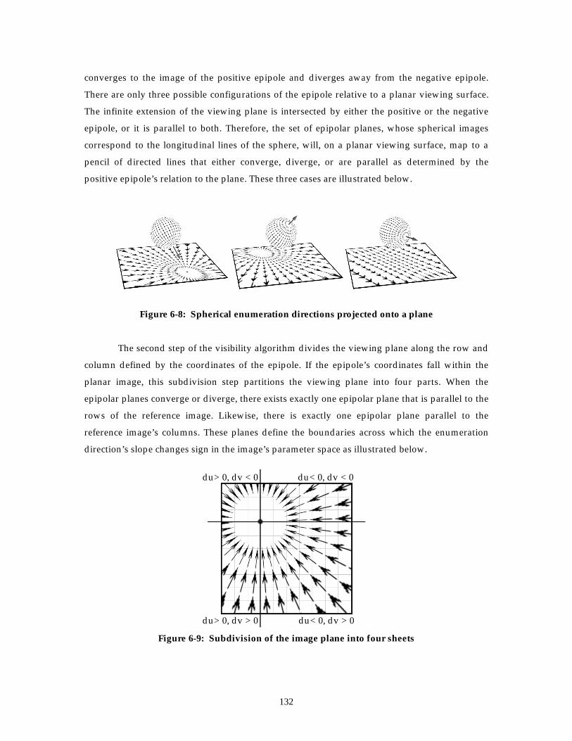
132
converges to the image of the positive epipole and diverges away from the negative epipole.
There are only three possible configurations of the epipole relative to a planar viewing surface.
The infinite extension of the viewing plane is intersected by either the positive or the negative
epipole, or it is parallel to both. Therefore, the set of epipolar planes, whose spherical images
correspond to the longitudinal lines of the sphere, will, on a planar viewing surface, map to a
pencil of directed lines that either converge, diverge, or are parallel as determined by the
positive epipole’s relation to the plane. These three cases are illustrated below.
Figure 6-8: Spherical enumeration directions projected onto a plane
The second step of the visibility algorithm divides the viewing plane along the row and
column defined by the coordinates of the epipole. If the epipole’s coordinates fall within the
planar image, this subdivision step partitions the viewing plane into four parts. When the
epipolar planes converge or diverge, there exists exactly one epipolar plane that is parallel to the
rows of the reference image. Likewise, there is exactly one epipolar plane parallel to the
reference image’s columns. These planes define the boundaries across which the enumeration
direction’s slope changes sign in the image’s parameter space as illustrated below.
Figure 6-9: Subdivision of the image plane into four sheets
du> 0, dv < 0 du< 0, dv < 0
du> 0, dv > 0 du< 0, dv > 0

133
The various enumeration orders of the visibility algorithm can be derived by
considering the signs of the directed lines’ slopes in each subregion. If one coordinate of the
epipole falls outside of the parameter domain, then the region is divided into two subregions. If
both coordinates fall outside of the parameter domain, then all of the enumeration directions
along the epipolar planes will have a common direction. This last condition corresponds to the
single-sheet case of the algorithm.
The final step in mapping the spherical-viewing-surface algorithm onto a planar viewing
plane is determining the order of enumeration. It is clear that points on the planar surface can be
reprojected along the epipolar planes and that the result would be consistent with the spherical
reprojection. This result would correspond to mapping the original planar image onto a
spherical projected image with the same center-of-projection, and then reprojecting the result
onto a new spherical frame. While this approach works, it is inconvenient since it involves extra
mapping steps. These steps can be avoided if the enumeration order is specified in the planar
parameter space. Next, I will show how enumeration along rows and columns of the viewing
plane used in the visibility algorithm presented in Chapter 3 is equivalent to enumeration along
the epipolar planes of the spherical viewing surface.
In the spherical case each longitudinal line, which corresponds to an epipolar plane, was
considered independently. In the modified planar case I will consider several epipolar planes
simultaneously. In the following figure a single subregion of the image plane is shown with two
directed isoparametric lines overlaid.
Figure 6-10:An equivalent enumeration along the rows and columns of a planar image

134
The overlaid vectors have the following properties. Each vector’s direction is consistent
with the spherical flow field’s projection onto the corresponding parameter axis. This direction
will be the same for all isoparametric lines in a given sheet since both components of the flow
field’s slope have a constant sign. A given isoparametric line will cross the projected image of
each epipolar plane in the subregion exactly once. If a series of these isoparametric lines are
enumerated in the direction of the flow field’s remaining component, then the overall image of
the spherical flow field is preserved. Furthermore, the relative ordering of the two parameters is
arbitrary.
By Theorem 1, multiplicities are constrained to occur only within epipolar planes. The
projected-spherical flow field is the image of these epipolar planes. If a series of isoparametric
lines are mapped in the transverse direction in the order determined by the sheet’s slope
component, then each point along the epipolar plane will be reprojected in order of decreasing
θ . This relative ordering is independent of the u or v parameter choice. Theorem 2 proves that
such an ordering is occlusion compatible. Therefore, the resulting planar enumeration is
equivalent to mapping the planar viewing surface onto a spherical viewing surface and
performing the reprojection there. Thus, the planar algorithm given is also occlusion compatible.
The various partitions and enumeration orders of the planar visibility algorithm all arise
from parameterization on a planar viewing surface. The choice of a desired center-of-projection
determines both the subdivision boundaries as well as the number of sheets. The enumeration
direction relative to the epipolar ray’s image is determined by whether the image is of the
positive or negative epipole.
Now I will consider the case where the projection plane is parallel to the epipole. Since
the projections of all epipolar planes onto the planar viewing surface are parallel, these
projections can be considered a special partitioning case in which there is only a single sheet.
The parameterization still determines the enumeration order along isoparametric lines based on
the slope of the flow field induced by the image of the spherical frames’ lines of longitude. Even
though both of the epipoles project to infinity on the planar viewing surface, the direction from
the negative to the positive epipole is still well defined. The visibility algorithm will handle this
case correctly.

135
6.4 Discussion
Special cases of the visibility algorithm presented in this paper have been developed by
Anderson [Anderson82] and Adelson and Hodges [Adelson93b]. Anderson’s hidden-line
algorithm considered the case of height-fields rather than projective images. In a height-field the
surface’s range values are measured by their projection onto a basis vector that is orthogonal to
the parameter-space dimensions. In a perspective-projected image range values are measured
from the center-of-projection. A height-field is a useful representation for bivariate functions. It
is also notable that Anderson’s algorithm enumerates the surface in an order opposite of the
presented algorithm. This requires a representation of the periphery of the surface being drawn.
Anderson’s painting rule, which requires that a surface can never overwrite a surface point
which has already been written, is the opposite of maintaining only the last surface written at
each point. Anderson’s enumeration order has the advantage of never generating points that are
subsequently overwritten. This is reasonable considering that his algorithm was developed for
line-plotter applications where, unlike computer-graphics displays, once ink is drawn on the
paper it cannot be satisfactorily overwritten. This reduction in the number of writes, however,
comes at the cost of maintaining the auxiliary data structure representing the drawn surface’s
boundary. Depending on the implementation, the representation of the boundary buffer can
itself introduce problems. If the extents of the boundaries are represented using a sampled
representation, then quantization artifacts can introduce precision problems in future
comparisons. If the boundary curves are represented explicitly as line segments, the storage
requirement are potentially large.
Adelson and Hodges proposed a method for generating stereo pairs from a single
planar ray-traced image by reprojecting the right eye’s image to the left eye’s view. The
algorithm they describe is equivalent to the special case of the given visibility algorithm where
the epipolar ray is both parallel to the view plane and is oriented along an isoparametric line of
the planar projection. This unique geometry allows for the right eye’s image to be generated by
enumerating and reprojecting the left eye’s image along all scan lines from left to right.
The given visibility algorithm can also be extended to other viewing surfaces by using
the same procedure of mapping the problem from the original viewing surface to a spherical
viewing surface, reprojecting it, and then mapping it back onto the original surface. The
following figure shows this progression of mappings on a cylindrical viewing surface.

136
Once more the longitudinal lines of the spherical projection correspond to the projected
images of the epipolar planes that are induced by a change in center-of-projection in the
direction of the epipolar ray. Images of these epipolar planes can be mapped onto a cylindrical
viewing surface that shares the same center-of-projection. The cylindrical projected surface can
then be reprojected along these lines of longitude in an order progressing from the negative to
the positive epipolar rays. The resulting enumeration would be equivalent to the spherical
reprojection which has been proven to be occlusion compatible.
Figure 6-11:A mapping of epipolar planes onto a cylindrical viewing surface
Using the method outlined above, visibility algorithms can be established for any
viewing surface that is topologically equivalent to a sphere (i.e., its range function is strictly
single valued). While this is the case for all perspective-projected images, it does not easily
extend to more general surface representations.

137
&KDSWHU �
COMPARING IMAGE-BASED AND GEOMETRIC METHODS
Despite the differences in scene representation, there are surprising similarities between
the rendering methods used for geometry-based and image-based computer graphics. Many of
these are a natural consequence of the common result shared by both approaches— an image.
However, the parallels between the two methods extend much further. In this chapter I
examine these two approaches side by side, with a focus on these similarities and differences.
There are tremendous advantages in leveraging the past twenty-five years of
accumulated expertise in graphics architectures as a starting point for image-based systems.
Recently, hardware architectures supporting geometry-based three-dimensional computer
graphics have made the difficult transition from a highly specialized add-on for high-end
computer systems to a commodity item for personal computers. In the near future there may be
considerable interest in adapting these built-in graphics capabilities for use in image-based
rendering. In the longer term the greatest potential for image-based computer graphics may lie
in hybrid systems capable of merging both modeling approaches.
The success of geometry-based computer graphics has, to a large degree, resulted from
breaking down the three-dimensional rendering problem into smaller manageable pieces. This
modular approach provides an invaluable organization for the rather daunting list of chores
required to convert a geometric specification into an image. It has also facilitated the
application of parallelism in the design of graphics systems and has therefore played a
significant role in enhancing performance.
While there is no single rendering approach used by all geometry-based computer
graphics systems, most can be classified as either primitive driven or display driven. Primitive-
driven methods traverse the list of scene elements, computing each primitive’s contribution to
the final image before proceeding to the next element. A display-driven approach progresses

138
through all of the sample points of the output image seeking those scene elements that
determine the sample’s value. Either of these techniques is applicable to the image-based
computer graphics method described here. The next two sections discuss these distinct
approaches and give analogous image-based methods.
7.1 The Image-Based Graphics Pipeline
In the primitive-driven approach to geometric computer graphics, model elements are
processed sequentially and, to a large extent, independently as they are converted from their
three-dimensional definitions into a sampled two-dimensional image. This transformation takes
place in several steps. The geometric elements are first tessellated into planar facets. Then, the
facets are transformed from the canonical modeling coordinate system of the geometric
primitive to the desired scene position. The color of the facet can be resolved once its position
relative to the viewing point and the illumination sources is known. If some part of the facet lies
within the field-of-view of a simulated camera, the three-dimensional coordinates of the facet’s
vertices can be projected onto the simulated camera’s viewing plane. With the image-space
coordinates of the facet’s vertices known, an image is computed by sampling the interior of the
facet at integer grid points. This list of operations makes up the standard graphics pipeline, as
illustrated below[Foley90].
Figure 7-1: Standard geometry-based graphics pipeline
The first stages of the graphics pipeline process geometric primitives. The operations
performed at these stages are primarily three-dimensional coordinate transformations that map
canonical geometric models to desired positions. The latter stages of the graphics pipeline
operate on image-space quantities. It is at this point that the minimal representation of the
geometry given by its vertex coordinates is converted into image-space samples representing
actual three-dimensional points.
ModelingTransforms
ViewingTransforms Projection Clipping
PerspectiveDivide
RasterSetup
ScanConvert

139
The warping phase of the image-based rendering method bears a close resemblance to a
three-dimensional transformation. In fact the standard 4 4× matrix multiplier of the graphics
pipeline could be used to compute the linear terms of the image warp given in Equation 3-16 as
follows:
x
y
w
w w w w
w w w w
w w w w
u
v
u v1 0 0 0 1
1
11 12 14 13
21 22 24 23
31 32 34 33
1
1
1 1
=
δ( , )
Equation 7-1: Using a 4 × 4 matrix multiplier to compute the image warp
The use of a matrix multiplier would not, however, take advantage of the coherence
available due to the sequential processing of reference image coordinates. In general only the
third column of the matrix needs to be computed for each pixel. The remaining terms can be
replaced with additions using the method of forward differences.
Following the linear-expression computations, an image-based rendering system would
test whether the w component of the transformed image point is positive, indicating that it is in
front of the pinhole camera. Once this is established, the remaining terms can be tested to see if
they fall into the valid range of image coordinates.
0 0≥ > × ≥ > ×x w width y w heightand
Equation 7-2: Image-based view port clipping
This series of tests is reminiscent of the clipping step in the traditional geometry-based pipeline.
The next stage of the image-based rendering approach divides both the x and y
components by w, just like in the projection stage of the geometry-based approach. The final
reconstruction and resampling processes of the image-based method are comparable to the
rasterization phase of the graphics pipeline. Standard rasterization hardware might even be
used to approximate the bilinear surface reconstructed when a C0 polynomial basis is used30.
Thus, a graphics pipeline can be defined for the image-based approach to computer
graphics as illustrated below.
30 This is only an approximation since a bilinear surface is not planar.

140
Figure 7-2: A image-based graphics pipeline
In the geometry-based graphics pipeline, visibility is usually determined at one of two
stages. Either the geometric primitives are presorted according to their distance from the
viewing position prior to the viewing transformation, or visibility is resolved on a sample-by-
sample basis during the rasterization process using the z-buffer algorithm.
The benefits of presorting-visibility methods are that they can take advantage of fast
sorting algorithms, they can be computed incrementally for animated sequences, and the
visibility solution is computed at a relatively high level of geometric representation. However, a
strict depth ordering on the basis of objects is difficult to define when scene elements
interpenetrate. Solving this problem usually requires significant geometric processing,
including the subdivision of scene elements. In general, presorting methods for computing
visibility are only considered for scenes with very few surfaces.
On the other hand, the z-buffer method for computing visibility generally works for any
configuration of objects because it considers geometry at the low level of points. Thus, the z-
buffering algorithm is tightly coupled with the sampling process. The major disadvantages of
the z-buffer method result from breakdowns in the underlying assumptions made during the
sampling process. For instance, most z-buffering algorithms consider the entire sampling region
to be represented by a single depth value. Yet, it is possible that several actual surfaces at
various depths might be represented within a sampling region. This is particularly noticeable
along object silhouettes and along curves where surfaces interpenetrate. Z-buffering methods
are the most common method used for resolving visibility in scenes composed of a large
number of surface elements.
The image-based method of resolving visibility most closely resembles the geometry-
based presorting approach. However, in the image-based case, this sorting is trivially computed
Warping Equation ClippingProjectiveNorm alize
Find SplatKernel
ScanConvert

141
since it can be determined without any geometric knowledge of the elements being rendered.
The resulting drawing order of the reference image is simply a function of the pinhole camera
model and the change in the center-of-projection between the reference and desired images.
Furthermore, the scene representation used in image-based rendering does not allow
interpenetrating scene elements. Thus, both the computational expense of computing an object
ordering and the special case handling of the geometry-based representation are absent from the
image-based approach.
7.2 An Inverse-Mapped Approach to Image-Based Rendering
The classical display-driven approach to geometry-based computer graphics is the ray-
casting method described by Appel [Appel67] and enhanced by Whitted [Whitted80]. From the
standpoint of a system architecture, the identification of distinct processing steps in the display-
driven computer graphics approach is not nearly as developed as in the primitive-driven
approach. Most systems, however, share the common algorithmic structure shown in Figure 7-
3.
A significant step in the display-driven approach to geometry-based computer graphics
is the mapping of a pixel coordinate to a three-dimensional ray. This ray is used in the
geometric calculations necessary for determining the visible scene primitives. A similar step can
be identified for the image-based approach. The fundamental matrix relating points in the
desired image to lines in the reference image can be determined using either pinhole camera
parameters (i.e., by taking the transpose of Equation 5-10,
F P P P21 21
1 2 21
1= −− −( ( ( � � )) )skew C C T ), or by using image correspondences and Hartley’s
method [Hartley95a] as discussed in Chapter 5. Alternatively, the nonlinear methods of Luong
[Luong93b] could be used.

142
Figure 7-3: Algorithm for a display-driven rendering approach
The product of a fundamental matrix with a desired pixel coordinate gives the equation
of a line through the reference image, as illustrated below.
Figure 7-4: Projection of a desired ray onto a reference image
This line is the projection onto the reference image of the ray emerging from the desired image’s
center-of-projection and passing through the identified point.
1) foreach pixel of the desired image2) determine the ray specified by the pixel3) set distance to closest intersection = large value4) set visible point = background5) foreach scene primitive6) if the ray intersects the primitive then7) compute distance along ray of intersection8) if distance to intersection < closest and9) distance to intersection > 0 then10) set visible point = point of intersection11) set closest = distance12) endif13) endif14) endfor15) Illuminate visible point16) set pixel = intensity of illumination at point17) endfor
Desired Image Reference Image
(u2,v2)
A u1 + B v1 + C = 0
A
B
C
u
v
=
F12
2
2
1

143
The precise segment along this line can be computed by examining the limits of the
warping equation given in Equation 3-1031. The maximum image-space extent along the ray
corresponds to the case when the generalized disparity value approaches zero since generalized
disparity is inversely related to range. Thus,
∞−=x xP P11
2 2
Equation 7-3: Maximum extent of epipolar line segment
Similarly, the minimum extent along the line segment occurs when the generalized disparity
value approaches infinity. The coordinate of this point in the reference image is given by
0 11
2 1x C C= −−P ( � � )
Equation 7-4: Minimum extent of epipolar line segment
The coordinate of the minimum extent is independent of the selected sampling point from the
desired image. This point is the epipole of the desired image as seen by the reference. In other
words it is the projection onto the reference image of the desired image’s center-of-projection.
The identification of the ray’s extents is analogous to setting the maximum ray distance in Step 3
of the ray-tracing algorithm and testing for the positive ray length in Step 9. This process is
shown in the following figure.
31 In order to preserve the notions of the reference image and the desired image in this case, the
sense of the warping equation is inverted.
Desired Image Reference Image
(u2,v2)0 x
∞ x
0 11
2 1
11
2
x C C
x
= −=
−
∞−
P
P P
( � � )

144
Figure 7-5: Endpoints of a ray in a reference image
Either or both of the ray’s endpoints might lie outside of the reference image’s
coordinate range. Furthermore, the sign of the third component of the two endpoints,
0 0 1 0 2 0 3x x x x T=[ , , ] and ∞ ∞ ∞ ∞=x x x x T[ , , ]1 2 3 , must be examined in order to properly
determine the ray’s direction of propagation within the image. The following cases can occur:
1) If both 0 3x and ∞ x3 are positive, the desired center-of-projection falls in front of the
reference image, and the ray intersects an extended image plane32 propagating from
0 x to ∞ x . The valid extent of the epipolar line is the segment connecting 0 x to
∞ x in the reference image.
2) If 0 3x is positive and ∞ x3 is negative, the desired center-of-projection also falls in
front of the reference image, but the ray does not intersect an extended image plane.
In this case the ray propagates from 0 x to a point out of view. The valid extent of
the epipolar line is the half-line from 0 x in the direction opposite of ∞ x .
3) If 0 3x is negative and ∞ x3 is positive, the desired center-of-projection lies behind
the reference image, and the ray intersects the extended image plane. In this case
the ray propagates from some point out of view to ∞ x . The valid extent of the
epipolar line is the half-line ending at ∞ x in the direction opposite 0 x .
4) If both 0 3x and ∞ x3 are negative, the desired center-of-projection lies behind the
reference image, and the ray does not intersect the extended image plane. All such
rays can be ignored since no point visible in the reference image falls along their
extent.
The intersection of the projected ray’s valid extent with the segment of the epipolar line visible
within the image gives the actual ray’s extent within the reference image.
Having identified two points on an epipolar line in the reference image, 0 x and ∞ x ,
we can always find any other point on the line by
32 The extended image plane is an unbounded plane that is both parallel to the actual viewing
plane and an infinite distance from the origin. Exactly half of the rays emerging from any point intersecta given extended plane.

145
p t xt x t( ) ( )= + −∞0 1
Equation 7-5: A parametric form of a line
where the parameter t is allowed to vary from -∞ to +∞. This represents the points on the line as
a linear combination of the two endpoints. If we substitute t = +τ
τ1 , the following alternative
representation results:
p x x( )ττ
τ τ=
++
+∞0 1
1
1
Equation 7-6: The tau form of a line
The new interpolation variable, τ , is consistent with the generalized disparity values δ( )x1 at
the two extremes (i.e., when τ δ= =( )x1 0 then p x( )0 = ∞ , and when τ δ= = ∞( )x1 then
p x( )∞ =0 ). Therefore, if the reference image point ∞ x is visible at our desired image point, it
is must have a disparity value of 0. Likewise, for the reference image point 0 x to be visible at
our desired image point, it is must have a disparity value of +∞. The necessary value
ofδ τ( ( ))p can be found for all points on the line by first solving either expression in Equation 3-
Z for δ( , )u v .
δ
δ
( , )( )
( , )( )
u vw u w v w u w u w v w
w u w
u vw u w v w v w u w v w
w v w
1 111 1 12 1 13 2 31 1 32 1 33
34 2 14
1 121 1 22 1 23 2 31 1 32 1 33
34 2 24
=+ + − + +
−
=+ + − + +
−
Equation 7-7: Disparity required to map a reference point to a desired point
Then, solve Equation 7-6 for τ .
τ
τ
( , )( ( ))
( )( )
( , )( ( ))
( )( )
u vw w u w v w u w u w v w
w u w w u w v w
u vw w u w v w v w u w v w
w v w w u w v w
1 134 11 1 12 1 13 2 31 1 32 1 33
34 2 14 31 1 32 1 33
1 134 21 1 22 1 23 2 31 1 32 1 33
34 2 24 31 1 32 1 33
=+ + − + +
− + +
=+ + − + +
− + +
Equation 7-8: Theta value at a point on the ray’s extent
Clearly, the relationship of δ( , )u v to τ is

146
δτ
( , )( , )( )
u vu v w u w v w
w1 11 1 31 1 32 1 33
34
=+ +
Equation 7-9: Minimum disparity required for a given tau value
Therefore, given any point on the actual ray’s extent within a reference image, the value
of τ for that point can be computed using either expression of Equation 7-8. For the best
results, the first expression should be used when the epipolar line’s slope has an absolute value
less than 1, and the second expression should be used otherwise. The value of the generalized
disparity which would make this same point visible along the ray is given by solving Equation
7-9 with the value of τ computed for the point. The full desired image can be computed as
follows:
Figure 7-6: Display-driven image-based rendering
Determining the generalized disparity value (Step 7) and the intensity value (Step 10) at
an arbitrary point in the reference image requires interpolation. This algorithm is analogous to
the ray-tracing algorithm given in Figure 7-6. It has an advantage over geometry-based ray-
tracing in that it traverses only a small fraction of the potentially visible points for a given ray. It
also traverses the reference image in such a way that the first intersection found is guaranteed to
represent the closest point.
7.3 Discussion
There are significant parallels between the rendering algorithms used for geometry-
based computer graphics and image-based computer graphics. In this chapter I have shown an
image-based rendering approach that has many similarities to the traditional three-dimensional
rendering pipeline. Likewise, I described an image-based approach that is similar to ray tracing.
1) foreach pixel of the desired image2) compute the epipolar line in reference image3) determine the projected ray’s actual extent4) foreach point along the propagation direction5) find τ at point6) find δ needed to see point7) if (δ at point) ≥ δ needed8) break;9) endfor10) set pixel = intensity at point11) endfor

147
In both cases when analogous functions were compared side-by-side, the image-based approach
was generally found to require fewer operations. Thus, as the number of geometric primitives
used to describe a scene approaches the number of pixels represented in an image of that scene,
we might expect that an image-based approach will outperform a geometry-based approach.

148
&KDSWHU �
CONCLUSIONS AND FUTURE WORK
The notion of a model is one of the most important concepts in computer graphics. It is
the job of a model to capture the essence of the concrete entity that it represents. While it is
important that a model remain true to the original, it is even more significant for a model to be
both simple and elegant. Geometric models are a perfect example of this assertion. We are
taught early on that geometry is but an abstraction. In our world, there are no dimensionless
points, no infinitely long and immeasurably thin lines, and no perfectly flat planes. Yet, we have
chosen geometry, with its simplicity and elegance, to represent those models that we hope to
visualize.
In the formative stages of computer graphics, the choice of geometric models was
indeed a clever optimization, because it allowed an uncountable number of surface points to be
specified using only a compact list of coordinates. But, as the field of computer graphics
advances, we are witnessing the erosion of this economy. Most practitioners would agree that
we are rapidly approaching the day when scenes composed of multiple millions of primitives
will be commonplace. In fact, one proposed measure of scene complexity is the ratio of
modeling primitives to the number of pixels rendered. In view of this, one might question the
logic of using three points to enclose a region of space whose projection is less than one pixel.
There are, however, other ways to represent objects for the purposes of visualization.
Images are particularly appealing because their visual source helps to form our expectation.
Most of us would agree that an image captures, from a single viewpoint, the visual essence of a
scene. Thus, all that is required is a method for transforming this essence to new viewpoints.
This research has presented just such a method.

149
8.1 Synopsis
In this thesis, I have contributed methods for transforming an image of a scene captured
from one point to an approximation of the scene as it would be viewed from some other point. I
have provided a framework for defining this approximation in the form of a plenoptic function.
I discussed a method for determining which of the transformed points would be visible in the
final image, along with techniques for representing a continuum of points when given only a set
of samples. Then, the notion of a camera was explored, and I explained how these rendering
techniques could be easily adapted to camera models which were either more flexible or more
realistic than the original planar-pinhole camera. The relationship of the rendering method to
the camera’s geometry was then explored, and I found that, in some cases, very little geometric
knowledge is required to synthesize reasonable images from others. Finally, the similarities
between geometry-based and image-based computer graphic systems were investigated. At the
system level many parallels between the two methods became apparent, and it was found that
image-based techniques often surpass the geometric methods. This is particularly true when the
number of primitives is comparable to the number of pixels in a reference image.
In the remainder of this chapter, I will concentrate on the specific advantages and
disadvantages of the image-based computer graphics approach presented here. I will then
cover limitations of the proposed methods. Finally, a wide range of open problems suitable for
future research are presented.
8.1.1 Advantages of image-based computer graphics
Overall performance of geometry-based computer graphics systems continues to
depend on the number elements composing a scene. Techniques for avoiding the unnecessary
processing of scene primitives that are either occluded or outside a desired image’s field-of-view
are an active area of research in geometry-based computer graphics. These techniques are
particularly useful in scenes with significant depth complexity. On the other hand, an image, by
definition, represents only a visible subset of a scene and has a depth complexity of exactly one.
For viewing positions nearby an image’s center-of-projection, it is reasonable to expect that there
will be only moderate changes in the visible scene elements.
The performance of an ideal image-based computer graphics system would be
proportional to number of pixels rendered rather than the number of primitives used in the
representation. In the forward-mapping case of image-based rendering, the computation

150
required is actually proportional to the number of reference image pixels used by the image
warp. When the resolution of the reference image is comparable to the desired image, and the
viewing positions are suitably close, then the performance is nearly ideal. However, the
performance of the forward mapping case cannot be considered independent of the model’s
representation, since surely we must consider the samples of a reference image as modeling
primitives. So, in the case of a forward-mapping image-based system, the primary performance
advantage results from the visibility preprocessing inherent in the image representation.
An inverse-mapping image-based system, though, can nearly approximate the
performance of an ideal system. Consider a reference image sampled at R × R resolution, and a
desired image with resolution of D × D. The computation required in the naïve algorithm
explained in Chapter 7 is proportional to D2αR, where D2 is the number of pixels in the image
and α is a constant that is generally less than one33. If a simple pyramid representation is used
for the reference image, it appears possible that this performance can be made proportional to
D2log(αR). Additionally, the pyramid might be used to address aliasing problems that are
common to display-driven methods.
Another computational advantage of image-based computer graphics methods is
derived from the spatial coherence of images. Many of the calculations involved in image
warping can be made incremental by using forward-difference techniques, since the underlying
representation is regular when compared to the nearly random configurations that geometric
primitives assume. A good example is the coordinate transformation used in both cases
discussed in Chapter 7. A geometry-based system uses a 4 × 4 matrix transformation to realize a
mapping of a three-dimensional point to an image-space coordinate (requiring at least 12
multiplies and 12 additions for the transform, plus 1 divide and 3 more multiplies for the
projective normalization). All of these operations are required because any point might occur
during the mapping. In contrast, the analogous mapping of two-dimensional reference image
points to image-space coordinates described in Chapter 3 requires, in the general case34, only 5
multiplies, 6 additions, and 1 divide. If we assume that three-dimensional triangles specified by
three vertices are used as primitives, then each will require 3×(15 multiplies + 12 adds + 1
division) operations per rendered pixel compared to the (5 multiplies + 6 adds + 1 division)
33 This assumes that some fraction of the projected ray’s extent will be clipped. In the case of a
stereo camera configuration (Chapter 3) α will exactly equal one. Note that it is also likely that a givenray will terminate early, thus further reducing the constant α.
34 Ignoring initial set up.

151
operations required for the image-based case35. Thus, even ignoring the advantage of a reduced
depth complexity, an image-based approach should outperform a geometry-based system when
each primitive contributes fewer than 3 pixels to the final rendered image.
A final advantage of image-based rendering is that photorealism is achieved with no
additional operations, since the photometric properties of a scene are determined entirely by
pre-computed values of the reference images (The inability of image-based systems to properly
represent view-dependent illumination artifacts, such as specular reflection, will be discussed in
the future work section). In modern geometry-based systems, the computational effort
dedicated to shading overshadows the geometric computations. In an image-based system,
shading can be considered as a preprocess that has no effect on the interactive performance.
This is similar to radiosity methods that are commonly used for geometry-based techniques.
However, radiosity methods will generally involve significantly more computation than image
acquisition.
8.1.2 Disadvantages of image-based computer graphics
In this section I will discuss many of the inherent drawbacks of the image-based
approach when compared with geometric methods. Other shortcomings are also identified and
considered in the future work section. However, I consider the problems discussed here nearly
insurmountable without major revisions in the approach.
Image-based models are non-metric representations; thus, while they are well suited for
the purpose of visualization, they not particularly useful as computational models. The
fundamental difficulty of this problem has long vexed the computer vision community. The
central goal of the classic structure-from-images problem has been to extract a model whose
validity is then judged against the standard of an abstract geometric representation36. My
approach, admittedly, uses many results that are generally well known among computer vision
researchers. However, it is my application of these results to the problem of mapping images to
images, rather than attempting to extract geometric models, that distinguishes my work. The
significance of a centimeter’s accuracy when either visualizing or analyzing a scene strongly
depends on where that centimeter falls relative to the viewer’s pose. This dependence,
35 The advantage of the image-based case increases if the reference pixel projects to more than
one pixel.
36 Like those used in traditional three-dimensional computer graphics.

152
however, is lost when accuracy is defined in terms of Euclidean measurements, rather than in
terms of the projective domain where the visualizations and the analyses occur.
Throughout this presentation I have ignored the temporal dimension of the plenoptic
function. The cost of considering time is particularly significant because it adds an entire
dimension to the plenoptic representation. Unfortunately, since this dimension is not geometric,
it is difficult to tailor the approximation process in terms of geometric constraints as was done in
the static geometry case. In contrast, it is relatively simple to define temporal behaviors for
geometric models. In the absence of some significant innovation it seems that image-based
methods are doomed to treat the time dimension as a database query problem.
Another disadvantage of using images as a representation for three-dimensional
computer graphics is that, unlike geometry, images constrain where a scene can be viewed from.
This problem is related to the lack of a metric representation, mentioned previously, but it also
encompasses the issue of visibility. An image does not represent points that cannot be seen, and
visible points are not represented equally. In contrast, a geometric representation of a
rotationally symmetric closed object represents more invisible points than visible ones37.
Furthermore, unless some view-dependent simplification method is used, all the points of a
geometric model are represented with comparable accuracy. These shortcomings appear to be
intrinsic to the image format.
8.1.3 Limitations of image-based methods
In this section I will discuss some of the limitations of image-based computer graphics
methods that arise in practice. Several aspects of the image-based approach, while theoretically
correct, suffer from sensitivities to errant inputs and singularities under certain geometric
configurations.
The image-synthesis methods discussed here depend on a generalized disparity defined
at every point on the image plane. While it is possible to obtain this disparity information from
correspondence information between images, the automated extraction of such correspondence
information is well known to be a difficult problem. An ideal system must also be able to
automatically determine this exact correspondence information. In practice the resolution
37 Due to perspective projection, generally, more than half of a closed surface will be obscured by
the remainder.

153
obtainable is limited by the sampling densities of the source images. Some of these problems
can be overcome with the appropriate technologies. For instance, the ambiguity problems of the
general correspondence problem can be minimized using structured light [Besl89]; the recovery
of disparities in occluded image regions can be overcome by considering multiple images
[Bolles87]; and approximate geometric models can be used to guide the correspondence process
[Debevec96]. The image-based approach is not bound to any particular method for establishing
correspondence, and therefore, it is well suited for hybrid combinations of methods. The
apparent quality of a scene’s representation is closely related to the accuracy of the disparity
information available. The quest for the accurate disparity information used in image-based
representations is akin to the difficulty of acquiring accurate three-dimensional geometric
models. Both problems have shown potential for automated solutions, but in practice, the
intervention of a human is generally required before satisfactory results can be attained.
The image-based approaches described are also subject to certain numerical
computation problems when confronted with noisy data. Most of these problems occur when
extracting information from sampled images. The computation of the fundamental matrix, as
described in Chapter 5, is known to be susceptible to noise [Luong93b]. It is also known that
there exist particular non-generic configurations of image points in which the solution is
singular [Torr95]. A similar situation occurs when solving the same-camera constraints. The
best approach to dealing with the singular configurations is to overspecify the system and use a
least-squares approach. This has the combined benefits of reducing the effects of noise, in the
case where it is uniformly distributed, and reducing the probability that a singular configuration
of points will arise. Unfortunately, an overspecification requires additional correspondence
information.
8.2 Future work
In this last section I will discuss future research directions and potential derivations
from the work presented in this thesis.
8.2.1 Sampling an environment
A principled approach for selecting a set of reference images is desperately needed. In my
opinion, there are at least three avenues worthy of exploration. The first approach would
involve searching for a global solution that attempts to assure that every point in a scene is well
represented. Such an approach might also consider external constraints on potential viewing
positions. For example, consider a game where the user is not allowed to crawl on the floor to

154
look at the undersides of furniture. Such a priori information might considerably reduce the
size of the image set needed to represent a scene. A second approach might focus on a local
solution that assures that some specific object or region of interest is well represented. This
approach appears to be closely related to the specification of an aspect graph [Plantinga90]. A
third potentially useful approach involves determining incremental solutions. Such an approach
can be summarized as follows: given N reference images, what single additional image would
most increase the usefulness of the model? This last approach appears similar to the way that a
human might approach the problem.
8.2.2 Reconstruction and resampling
Another interesting area for future research involves enhancing the reconstruction of a
continuous image representation prior to the resampling of the desired image, as discussed in
Chapter 3. One simple improvement would be to incorporate higher degrees of continuity
(estimates of the tangent space and curvatures at each point).
Another approach to this problem would be to devise a family of basis functions that
allows for varying degrees of connectivity throughout the image, permitting the selective use of
sparse (Gaussian-like) and dense (Polynomial-like) representations at various image regions.
Such an approach might be similar to the regularization techniques suggested by [Grimson81]
and [Terzopolous84]. These techniques employ multiconstraint optimizations to minimize some
energy function that is expressed as a weighted sum of different penalty and stabilizing forces.
Anisotropic diffusion models might also be applied to the reconstruction problem where the
local diffusion coefficient might be based on some estimate of a given point’s connectivity to its
surrounding neighborhood [Perona90] [Whitaker93].
8.2.3 Incorporating information from multiple reference images
In the ideal image-based computer graphics system, information missing from a warped
image would be filled in by warping some fraction of another image. The difficulty lies in
identifying what reference-image subregion will supply the missing data without actually
warping the entire reference image. Some preliminary work has been done by [Mark97] who
has found effective clipping algorithms that minimize the cost of subsequent warps. Also, the
inverse-mapping approach that is currently being explored by me and Bishop shows particular
promise in this area. The primary difficulty is to establish a good confidence estimate for any
reconstructed point. The confidence estimate in Mark’s approach requires additional geometric
information beyond a purely image-based representation. The method used in the inverse-

155
mapping case estimates the disparity gradient at each pixel to establish the confidence in a given
reconstruction. It is easy to construct examples where this measure is invalid (i.e., when actual
surfaces are nearly tangent to the visual ray). However, most of these errors result in a false
negative. Thus, there is still hope that a better reconstruction might be found in another
reference image if the surface is represented redundantly.
8.2.4 Image-based computer graphics systems
Identifying how systems might be built specifically for rendering image-based computer
graphics, or how existing geometry-based systems might be augmented to support image-based
methods is another interesting area for future research. An ideal system would need access to a
large database of reference images. Interesting problems include strategies for accessing and
caching images. Alternatively, image-based methods might be best served by accessing and
caching rays. Developing specialized hardware architectures for use in image warping and
reconstruction is one more promising area for additional research. Furthermore, there is
significant potential for parallelism when warping since only the image points on the same
epipolar line can possibly interact.
8.2.5 View dependence
The image-based computer graphics methods described in this thesis map the
photometric observations from one viewing position to any other viewing position. However,
the intensity of light reflected from a surface point generally varies according to the direction of
observation. This view-dependent distribution of the outgoing light that is reflected from a
surface is called a surface’s radiance function. The approach taken in this research makes the
assumption that the radiance function of all surfaces is well represented by a uniform
distribution over the hemisphere surrounding a point. Such a surface model is called an ideal
Lambertian reflector.
It might be possible, however, to incorporate a surface’s radiance function into the
plenoptic model. Furthermore, it appears likely that such an extension might be accomplished
with only slight modifications of the plenoptic function’s representation. Consider the following:
the subspace of a plenoptic function defined at any point in space describes the set of impinging
rays, whereas the radiance function describes the rays emanating from a point. Both functions
can be parameterized using two angles to indicate each ray’s direction. Moreover, the useful
regions of the plenoptic function, for the purpose of visualization, are the empty points of the
represented environment. In contrast, a radiance function is only defined at occupied points

156
within the space (assuming that there is no participating medium such as smoke). Consequently,
there is no practical overlap of these two functions. Therefore, any general representation of a
plenoptic (radiance) function can be potentially extended to incorporate radiance (plenoptic)
information without increasing the dimension of the representation. It also seems likely that an
interpolation method could be developed to incorporate information from both function types.
An alternative approach for incorporating view-dependent effects into an image-based
computer graphics system involves replacing the photometric values of a reference image with a
complete material specification. Such an approach might use the warping equation to map
reference image points to their position in the desired image, while deferring the shading
calculations until the final visibility is resolved. The primary difficulty of this type of approach
appears to be the acquisition of suitable models.
8.2.6 Plenoptic approximation methods other than warping
Image warping is just one possible approach for reconstructing a plenoptic function
from a series of images. Other researchers [Levoy96] [Gortler96] have suggested alternatives
that depend largely upon queries to a database of rays in order to reconstruct the desired
images. The disadvantage of the warping approach is that it requires the image to be augmented
with additional information that represents the projective structure of the actual points within
the space. The database approach, on the other hand, is data intensive. It has been argued that
there is tremendous potential for compression in the database approach. I would suggest that
this potential is maximized only when the algorithm used for the compression is cognizant of
the geometric structure of the scene being represented. This leads back to a more image-
warping-like approach. It also seems likely that a hybrid of the warping and database systems
could be built to take advantage of each approach’s strengths.
There may also be tremendous potential in exploring alternate interpolation bases for
the plenoptic reconstruction problem. Since the function is naturally represented as a field of
spherical subspaces, a spherical wavelet representation appears to be a particularly promising
area for future exploration.

157
Appendix A
NONGENERIC FORMS OF THE FUNDAMENTAL MATRIX
Usually a fundamental matrix can be described using Equation 5-5. However, there exist
nongeneric camera configurations that cannot be expressed in this form. These exceptional cases
correspond to having at least one of the two image planes parallel to the line connecting the
centers-of-projection. This condition can be recognized when the determinant of the upper
submatrix is zero ( f f f f11 22 12 21 0− = ). In real-world applications, it is unlikely that such
configurations will occur. These exceptional cases are presented here primarily for completeness
and so that suitable tests for detecting these configurations can be identified38.
In the general case of a fundamental matrix, the epipoles of each image have a proper
projection onto the other image. Such epipoles are considered finite, and their homogeneous
representations can be projectively normalized. In the exceptional cases of the fundamental
matrix, one or both of the epipoles are infinite. Thus, they are represented by a projective vector
with a zero-valued projective component. These points lie on the so-called line at infinity
defined for the projective plane. When these points are interpreted using the planar or flat model
of projective space, they are considered as pure directions rather than actual points [Coxeter74]
[Stofi91]. The implication of such configurations on the epipolar geometry is that the rays from
one center-of-projection project onto the other image as parallel lines. The slope of these lines is
given by the ratio of the two nonzero projective coordinates, and, in the projective sense, they
are considered to intersect at infinity.
The first parameterization for a nongeneric fundamental matrix considers the case when
only one of the two epipoles is infinite and the f11 element is non-zero. The canonical form of this
38 It should also be noted that the nongeneric epipolar geometries described by the special forms
of the fundamental matrix are artifacts of a planar viewing surface. Most of these cases are eliminated,and certainly less likely to occur, when a panoramic viewing surface is considered.

158
representation assumes that the fundamental matrix has been scaled so that its f11 element is
one. The following six-parameter model results:
F
e
e
e
e q r s
e e
e
eq
rbe
es
u
v
u
v
u v
u
v
u
v
21
1
1
2
2
2 2
1
1
1
10 1
1
0
0
11
�
=− −
−
−
, , , ,
Equation A-1: Model for a fundamental matrix with one finite and one infinite epipole
The curved circumflex symbol indicates which image-space contains the infinite epipole. The
case of a single infinite epipole in the first image with epipolar lines having a nonzero slope is
indicated when f f f f11 22 12 21 0− = and f f f f21 32 22 31 0− = 39. An infinite epipole in the
second image that also has epipolar lines with a nonzero slope is indicated when the same set of
conditions occurs in the fundamental matrix’s transpose. Equation A-1 describes a six-
dimensional subspace of linear transforms because any scalar multiple of the infinite epipole
will result in the same fundamental matrix. This is consistent with a geometric interpretation of
an infinite epipole as a pure direction, which can be specified by a single angle.
A five-parameter model of the fundamental matrix arises when the slopes of the
epipolar lines are equal to zero. A model for this case is given below:
F
e e
e q r
e e
q ru u
v
u v
q21
1 2
2
2 2
10
0 1
1
0
0
10
0 1 0
0 0 1�
=− −
−
, , , ,
cos sin
sin cosθ
θ θθ θ
Equation A-2: Fundamental matrix with one finite and one zero-slope infinite epipole
The breve symbol is used to indicate an image-space that contains a zero-slope infinite
epipole. The zero-slope case of a single infinite epipole in the first image is indicated when the
single-infinite-epipole condition ( f f f f11 22 12 21 0− = and f f f f21 32 22 31 0− = ) is caused by
zeros in the leftmost column of the fundamental matrix. In such a configuration, the f11 element
cannot be normalized by scaling. A zero-slope infinite epipole in the second image is indicated
by a topmost row of zeros.
39 Equivalently, this condition is indicated when the right-side vector associated with the singular
value of the fundamental matrix’s singular-value decomposition has a third element of zero.

159
When the epipoles of both images are infinite and have nonzero slopes, the following 5-
parameter model can be used for the fundamental matrix:
F
e
e
e
e q r s
q r
su
v
u
v
ee
eeu
v
u
v� �
21
1
1
2
2
0 0
1 0
01
0 0 12
2
1
1
=
−−
, , , ,
Equation A-3: Fundamental matrix with two non-zero-slope infinite epipoles
This nongeneric condition is indicated by a fundamental matrix with a nonzero f11 value in
which f f f f11 22 12 21 0− = , f f f f21 32 22 31 0− = , and f f f f12 23 22 31 0− = .
The following four-parameter model can be used to represent an epipolar geometry
with two infinite epipoles in which the epipolar lines of the first image have a zero slope.
F
e e
e q r s
q
r
s
u u
v
ee
bee
u
v
u
v� �
21
1 2
20
0 0
10 1 0
0 0 12
2
2
2
=
− −, , , ,
Equation A-4: Fundamental matrix with a non-zero slope and a zero-slope infinite epipole
This condition is indicated by a fundamental matrix with a leftmost zero-column and a nonzero
f12 value. Two infinite epipoles with zero-slope epipolar lines in the second image are indicated
by the same conditions applied to the given fundamental matrix’s transpose.
A final three-parameter model of the fundamental matrix can be used to characterize the
case when the epipolar lines of both images have a zero slope and both epipoles are infinite.
Such a matrix is indicated when both the leftmost column and topmost row of the fundamental
matrix are zero. Such a fundamental matrix can be normalized by scaling the matrix by the
reciprocal of the squareroot of the determinant of the lower-right submatrix (causing the
resulting submatrix to have a determinant of one). A model for this nongeneric situation is given
below:
F
e e
q rq ru u
q
� �
21
1 2
10
0
0
0
0
1
0
0
0
10
0 1 0
0 0 1
=
−
, , , ,
cos sin
sin cosθ
θ θθ θ
Equation A-5: Fundamental matrix with two zero-slope infinite epipoles

160
In such a configuration, the epipolar lines of both images will correspond to the scan
lines (i.e., isophotes of constant v) of both images. Notice that this arrangement is identical to the
stereo-camera condition depicted in Figure 3-4. Therefore, depth-from-stereo methods, which
depend on mechanical calibration, rely upon a particularly nongeneric camera configuration (a
3-dimensional subspace of a generally 7-dimensional problem). As a result, they should be
expected to be very sensitive to any external system noise.

161
Yes
Yes
Yes
YesYes
No
No No
No
Appendix B
SPECIAL CASES OF THE CLOSED-FORM
SAME-CAMERA SOLUTION
In Chapter 5 a method was derived for computing the intrinsic parameters of a non-
skewed planar-pinhole camera from a projective transformation, C , that satisfies the same-
camera constraints given by Equation 5-23. A closed-form solution for the camera’s intrinsic
parameters was presented for all cases except when c31 0= and c32 0= . Generally, these
conditions are unlikely because they comprise a two-dimensional subspace within the seven
dimensional space of same-camera transforms. For completeness, however, these special cases
of the projective transform, C, are addressed in this Appendix.
The various special cases of C are depicted in the following diagram:
Figure A-1: Diagram of the special case solutions
First, I will consider the special case of same-camera projective transformation where
c31 0≠ , c32 0= , and c12 0≠ . The Euclidean metrics of such a camera can be expressed as
follows:
c31 0=
c32 0= c32 0=General Case:Eqns 5-29, 5-30 and 5-31
c12 0=Special case B-1 Special case B-2 Special case B-3 Special case B-4
Special case B-5
c21 0=
No

162
b bc
c
a cc z c c c b b z c c
c c
b cb b z c z c
c
c cb b c c a c c b c c c
c
⋅ =−
⋅ = − − ⋅ +
⋅ = ⋅ −
⋅ = ⋅ + ⋅ + ⋅ +−
122
222
12 22 22 11 22 21 22 21
12 31
21 22 22 21
31
232
33 13 23 132
332
1
2
1
( ) ( )( )
( )
( ) (( ) ( ) )
Equation B-1: Solution for camera metrics when c31 0≠ , c32 0= , and c12 0≠
When c31 0≠ , c32 0= , and c12 0= the vector b b⋅ cannot be determined; however,
the remaining Euclidean metrics can be solved for as follows:
a cc z c
c z
b ca c c c c c c c c c c c
c c z c
c ca c c c c c c c c c c c c c c c
c c z c
⋅ = −+
⋅ = ⋅ − − + − − −+ +
⋅ =⋅ + − + + − −
+ +
33 22 11
31 22
31 11 332
13 31 33 332
11 132
312
31 21 21 33
31 11 23 33 13 21 33 33 112
23 23 132
21 31
31 21 21 33
1
2 1 1 1
1
2 1 1
( )
( ) ( ( ) ) ( )( )
( )( )
( ) ( ( ) ) ( )( )
( )( 1)
Equation B-2: Solution for camera metrics when c31 0≠ , c32 0= , and c12 0=
This situation arises when the camera’s axis of rotation is aligned with one of the basis vectors of
the image plane.
The next special case considered occurs when c31 0= , c32 0≠ , and c21 0≠ .
b bc
c
a cc z b b c z
c
b cb b c z c c z c c
c c
c cb b c c a c c b c c c
c
⋅ = −
⋅ =− ⋅
⋅ = ⋅ − − −
⋅ =⋅ − − ⋅ + ⋅ −
1
1 2
112
212
11 12 21 11
32
11 11 22 112
12 11 12
21 32
222
32 12 22 122
322
( )
( )( )
( )( ) (( ) ( ) )
Equation B-3: Solution for camera metrics when c31 0= , c32 0≠ , and c21 0≠

163
The condition when c31 0= , c32 0≠ , and c21 0= can also occur when the camera’s rotation
axis is aligned with one of the image-space basis vectors. In this case the following solution
arises:
( ) ( ) ( )( )
( ) ( )( ) ( ) ( )( ) ( )( )
( )( )
b bz a c c c c c c c c z c c c c c c
c c z c
a cc
c
b ca c c c c c c c c c c c c c c c c c c
c z c c
c cb b c
⋅ =⋅ + ⋅ − + −
−
⋅ = −
⋅ =⋅ + − − ⋅ − − − + + + −
−
⋅ =⋅ − −
2
2 1 1 1 1
2
1
13 32 33 32 22 33 11 122
23 33 132
22 32
23 33 11 22
12
32
12 232
32 13 33 222
222
332
232
322
332
122
232
132
222
23 11 22 33
222 ( ) ( )( )2 32 12 22 12
2
322
c a c c b c c c
c
⋅ + ⋅ −
Equation B-3: Solution for camera metrics when c31 0= , c32 0≠ , and c21 0=
When c31 0= and c32 0= the resulting projective transformation is affine. In this case
the vector c c⋅ cannot be determined; however, the remaining camera metrics can be solved for
as follows:
( ) ( )
( )( )
b bc c
c c
a cb b c c c c
c c
b cc c c b b c
c c
⋅ = −
⋅ =⋅ − −
− −
⋅ =− ⋅ −
− −
11 12
21 22
21 23 13 11
11 22
12 13 23 22
11 22
1
2
1
2
Equation B-5: Solution for camera metrics when c31 0= and c32 0=

164
Appendix C
FINDING CAMERA MODELS IN IMAGES
WITH COMMON EPIPOLES
The typical case in which a pair of images have the same epipole coordinate arises when
a camera is translated without rotation, as depicted in the following figure:
Figure C-1: A typical camera configuration leading to common epipole coordinates
The same-camera surface parameterizations given by Equations 5-34, 5-35, and 5-37 are
degenerate in this case. Such configurations are common enough, however, to deserve special
treatment. A second less likely case of a pair of images having the same epipolar coordinate
occurs when the rotational axis and the translation direction are coincident. This situation is
shown in Figure C-2. The methods developed in this Appendix apply to both of these cases.

165
Figure C-2: A second configuration leading to common epipole coordinates
When an image pair has common epipole coordinates (a state that can be determined by
a fundamental matrix and its transpose having the same point in their null spaces), the trace of
the compatible matrix can be expressed in terms of its determinant as follows :
TraceDeterminant
( )( )
σσ
σσ
σσH
HF
F= + = +2 3 2 3
1m m
Equation C-1: Value of trace when the epipole coordinates are the same in both images
This can easily be seen by equating the epipoles in Equation 5-34 and Equation 5-35.
Furthermore, if Equation 5-34 is solved for the parameter h33 and substituted into the
trace-equals-the-sum-of minors equation, all dependence on the remaining two parameters, h31
and h32, cancels out and the following expression results:
( )( )( )σ σ σ σσ
− + − +=
1 1 10
23
2
m
Equation C-2: Values of σ that potentially satisfy the same-camera constraints
Since a non-zero value of σ is required for the projective transformation to have a unit
determinant, we need only consider the four roots of the numerator as potential scaling factors.
Substituting these values into Equation C-1 and verifying the remaining relational constraint of
the same-camera transformation gives

166
− ≤ ± ≤− ≤ − ± − ≤
1 1 3
1 1 4 33
3 32
m
m m
Equation C-3: Valid ranges for the trace of the projective transform
With the exception of the points m3 2= ± there is no common overlap between these two
solution sets. The first relationship applies when m3 2≤ , while the second relationship applies
when 2 2 5 2 2544033≤ ≤ + ≈m . . All other values for m3 do not allow for a valid same-
camera solution. Thus, frequently only two of these four solutions need be considered.
The angle of the camera’s rotation can be directly determined from the trace, which in
this case has one of four possible values:
θ ∈ − +
− −
− − −Arccos Arccos Arccos Arccos( ), ( ), ,m m m m m m3 3 3 32
3 32
2 24
24
21 1
Equation C-4: Rotation angles
In the typical translation-only case depicted in Figure C-1 m3 2= (recall that
m f f3 21 12= − and, in the case of no rotation, F I= Skew( )e2 ). In this situation the rotation
angles reduce to { }θ π= 0, . In most applications, only the rotation angleθ needs to be
considered since generally a pair of translated cameras whose orientation varies by π radians
will see no points in common, with an exception occurring when the epipole is within the field-
of-view.

167
Appendix D
AN EXAMPLE IMAGE-BASED SYSTEM
D.1 Overview
This Appendix provides source code for an example image-based computer graphics
system written in the Java programming language. This image-warping implementation
assumes a planar-pinhole camera model for both the reference and desired images. It also
supports multiple reference images. Each reference image is stored in JPEG compressed format
while the associated disparity data is stored as a gray scale GIF image that has been scaled and
quantized to 256 levels. An example HTML file for invoking the image warper is shown below.
<HTML><HEAD><!-- created: 04/03/96 by Leonard McMillan --><TITLE> Image-Based Computer Graphics Applet</TITLE></HEAD><BODY><H1> Image-Based Computer Graphics Applet </H1><HR><CENTER><APPLET code="Vwarp.class" width=400 height = 400><param name="numrefs" value=4><param name="reference0" value="proja.jpg,proja.gif,0,-36,36, -22.745,45.2376,4.78461,0.142156,0,0, 0,-0.057735,-0.129904, 0.529088,1.31943"><param name="reference1" value="projb.jpg,projb.gif,-23.1403,-27.5776,36,11.6545,49.2742,4.78459, 0.108898,-0.0913759,0, -0.0371113,-0.0442276,-0.129904,0.000615401,1.32566"><param name="reference2" value="projc.jpg,projc.gif,-9.98,-27.44,41.71, -5.4776,46.3995,-4.85222, 0.123386,-0.0448759,0, -0.0267762,-0.0736211,-0.105361, 0.398979,1.30172"><param name="reference3" value="projd.jpg,projd.gif,40,6,32, -43.2382,-31.1167,11.3524, -0.0225834,0.150556,0, 0.0428222,0.00642333,-0.145952, 0.366496,1.43569"><param name="move" value=2><param name="fov" value=60></APPLET></CENTER><HR></BODY></HTML>
Each reference image is specified by a parameter string with a name of the form
“referenceX," where X is the index of the reference image. The first two arguments of the
parameter’s value specify the names of the image and disparity files. The following three
numbers of the comma separated string define the coordinates of the image’s center-of-

168
projection. The next nine numbers define the projection matrix for the planar image-space to ray
mapping function in row-major order. The last two numbers specify the minimum and
maximum disparity values represented by the 256 levels of the disparity image.
D.2 Modules and Classes
The example planar image warper is partitioned into five files with the following contents:
Vwarp.java contains the central applet which implements separate threads for the image warper and theuser interface.
Reference.java defines a generic interface for a reference image.PlanarReference.java contains an implementation of a planar reference image with warping methods. Italso implements a PlanarView which encapsulates all of the pinhole-camera information associated witha planar reference image.
Vector3D.java provides general vector and matrix objects.Raster.java defines an interface to an image that allows pixels to be accessed randomly.
D.3 Source
The source code for each file is provided below.
D.3.1 Vwarp.java
import java.applet.*;import java.awt.*;import java.util.*;import java.awt.image.*;import PlanarReference;import Vector3D;
public class Vwarp extends Applet implements Runnable { final static float DEFAULT_FOV = 40; final static float DEFAULT_MOVE = 1;
int curRef; // index of current reference image int numRefs; // number of reference images available PlanarReference reference[ ]; // array of reference images Vector3D eyePoint; // desired center-of-projection Vector3D lookAt; // optical axis Vector3D up; // three-space vector that projects up float hfov; // horizontal field-of-view float moveScale; // size of step PlanarView currentView; // desired view point and projection Raster window; // display window Image output; // working image
// The init method is the first one executed when the applet is loaded public void init() { // Get the number of reference images try { numRefs = Integer.parseInt(getParameter("numrefs")); } catch (NumberFormatException e) { numRefs = 0; }
// read in the reference images reference = new PlanarReference[numRefs]; for (int i = 0; i < numRefs; i++) {

169
String refInfo = getParameter("reference"+i); if (refInfo == null) continue; StringTokenizer parser = new StringTokenizer(refInfo, " ,"); // get viewing parameters try { Image image = getImage(getDocumentBase(), parser.nextToken()); Image disparity = getImage(getDocumentBase(), parser.nextToken()); Vector3D O = new Vector3D(parser); // center-of-projection Vector3D Vp = new Vector3D(parser); // vector to image origin Vector3D Du = new Vector3D(parser); // x spanning vector Vector3D Dv = new Vector3D(parser); // y spanning vector float mind, maxd; mind = Float.valueOf(parser.nextToken()).floatValue( ); maxd = Float.valueOf(parser.nextToken()).floatValue( ); Matrix3x3 P = new Matrix3x3(Du, Dv, Vp); PlanarView view = new PlanarView(O, P); reference[i] = new PlanarReference(this, image, disparity, maxd, mind, view); } catch (NumberFormatException e) { System.err.println("Error: Invalid float value"); System.exit(1); } showStatus("Image["+i+"] size = " + reference[0].width + " x " + reference[0].height); }
// set default view curRef = 0; eyePoint = reference[curRef].getOrigin(); lookAt = reference[curRef].getCenter(); up = new Vector3D(0, 0, 1); hfov = DEFAULT_FOV; String fovval = getParameter("fov"); if (fovval != null) { try { hfov = Float.valueOf(fovval).floatValue(); } catch (NumberFormatException e) { hfov = DEFAULT_FOV; } } hfov *= Math.PI / 180;
moveScale = DEFAULT_MOVE; String moveval = getParameter("move"); if (moveval != null) { try { moveScale = Float.valueOf(moveval).floatValue(); } catch (NumberFormatException e) { moveScale = DEFAULT_MOVE; } }
window = new Raster(size().width, size().height); window.fill(Color.blue); output = window.toImage(this);
currentView = new PlanarView(eyePoint, lookAt, up, hfov, size( )); warpInfo(ENQUEUE, currentView); }
// the following variables permit the warper and// user interface to operate asynchronously protected final static int ENQUEUE = 0; protected final static int DEQUEUE = 1; protected int warpCount = 0; protected boolean warpOutstanding = false; protected PlanarView warpView, nextView; Thread warper;

170
// this method passes *recent* events to the warper thread protected synchronized boolean warpInfo(int action, PlanarView view) { boolean rval = true; if (action == ENQUEUE) { nextView = new PlanarView(view); warpOutstanding = true; warpCount += 1; } else if (action == DEQUEUE) { if (warpOutstanding) { warpView = new PlanarView(nextView); warpOutstanding = false; } else { rval = false; } } return rval; }
// spawn a separate thread for the warper public void start() { warper = new Thread(this); warper.start(); }
public void stop() { warper.stop(); }
// performs a warp if an event is pending public void run() { long time = 0; while (true) { if (warpInfo(DEQUEUE, null)) { window.fill(getBackground()); time = System.currentTimeMillis(); reference[curRef].Warp(warpView, window); time = System.currentTimeMillis() - time; output = window.toImage(this); paint(this.getGraphics()); } else { showStatus(time+"ms Waiting for input ["+warpCount+"]"); try { System.gc(); Thread.sleep(100); } catch (InterruptedException e) { break; } } } }
// copys the image to the display public void paint(Graphics g) { g.drawImage(output, 0, 0, this); }
// simplify redraws public void update(Graphics g) { g.setColor(getForeground()); paint(g); }
Vector3D V0; // vector in the direction

171
// of the initial mouse button press
// handle the pressing of a mouse button public boolean mouseDown(Event e, int x, int y) { V0 = Vector3D.normalize(currentView.map(x, y)); return true; }
// handle drags of the mouse while a button is held down public boolean mouseDrag(Event e, int x, int y) { Vector3D V1 = Vector3D.normalize(currentView.map(x, y)); Vector3D Axis = V1.cross(V0); Vector3D newLook = new Vector3D(lookAt);
// rotate the current look-at direction if (Axis.length() > 0.0001) { float angle = (float) Math.asin(Vector3D.length(Axis)); newLook = newLook.rotate(Axis, angle); }
// translate along the look-at direction if either // shift or control is pressed during the drag if (e.shiftDown()) { eyePoint = eyePoint.plus(V0.scale(moveScale)); } else if (e.controlDown()) { eyePoint = eyePoint.plus(V0.scale(-moveScale)); }
// update the current viewing matrix PlanarView view = new PlanarView(eyePoint, newLook, up, hfov, size( )); warpInfo(ENQUEUE, view); return true; }
// handle releases of mouse button public boolean mouseUp(Event e, int x, int y) { Vector3D V1 = Vector3D.normalize(currentView.map(x, y)); Vector3D Axis = V1.cross(V0);
// rotate the look-at vector if (Axis.length() > 0.0001) { float angle = (float) Math.asin(Vector3D.length(Axis)); lookAt = lookAt.rotate(Axis, angle); }
// translate if either the shift or control key was pressed if (e.shiftDown()) { eyePoint = eyePoint.plus(V0.scale(moveScale)); } else if (e.controlDown()) { eyePoint = eyePoint.plus(V0.scale(-moveScale)); }
// update the current view currentView = new PlanarView(eyePoint, lookAt, up, hfov, size( )); warpInfo(ENQUEUE, currentView); return true; }
// handle keyboard events public boolean keyDown(Event e, int key) { if (key == 'n') { // go to next reference image curRef += 1; if (curRef == numRefs) curRef = 0; warpInfo(ENQUEUE, currentView); } else

172
if (key == 'r') { // reset viewing parameters eyePoint = reference[curRef].getOrigin(); lookAt = reference[curRef].getCenter(); up = new Vector3D(0, 0, 1); currentView = new PlanarView(eyePoint, lookAt, up, hfov, size( )); warpInfo(ENQUEUE, currentView); } else if (key == 'w') { // display a wider field-of-view hfov *= 1.125f; currentView = new PlanarView(eyePoint, lookAt, up, hfov, size( )); warpInfo(ENQUEUE, currentView); } else if (key == 'z') { // zoom into the current field-of-view hfov *= 0.88888888f; currentView = new PlanarView(eyePoint, lookAt, up, hfov, size( )); warpInfo(ENQUEUE, currentView); } return true; }}
D.3.2 Reference.java
import java.awt.*;import java.awt.image.*;import java.util.*;import Raster;
public class Reference extends Raster { protected float maxDisparity, minDisparity;
// Constructor public Reference(Component root, Image img, Image dsp, float maxd, float mind) { super(img); // get the image pixels Raster dspras = new Raster(dsp); // get the disparity values
// determine the pixel buffer's width and height if ((dspras.width != width) || (dspras.height != height)) { System.err.println("Error: image and disparity are of different sizes"); return; }
// copy the disparity information into the pixel array
for (int p = 0; p < pixel.length; p++) { int rgb = pixel[p] & 0x00ffffff; int d = dspras.pixel[p] & 0x0000ff00; pixel[p] = (d << 16) | rgb; }
maxDisparity = maxd; minDisparity = mind; }}
D.3.3 PlanarReference.java
import java.awt.*;import java.awt.image.*;import java.util.*;import Reference;import Vector3D;import Raster;
public class PlanarReference extends Reference { protected Vector3D Du, Dv, L; protected PlanarView view; protected float K[][]; protected float splat;

173
// Constructor public PlanarReference(Component root, Image img, Image dsp, float maxd, float mind, PlanarView v) { super(root, img, dsp, maxd, mind); view = v; K = new float[256][3]; }
// Methods public Vector3D getOrigin( ) { return view.origin( ); }
public Vector3D getCenter( ) { return view.map(width/2, height/2); }
// the actual warping is done in this method private protected void sheet(PlanarView outView, Raster output, int u0, int u1, int v0, int v1) { int du, dv; float dr, ds, dt; float drdu, dsdu, dtdu; float drdv, dsdv, dtdv; float lr, ls, lt; float kr, ks, kt; float dblW, dblH;
dblW = (float) output.width; dblH = (float) output.height;
if (v1 >= v0) { dv = 1; drdv = Dv.x; dsdv = Dv.y; dtdv = Dv.z; } else { dv = -1; drdv = -Dv.x; dsdv = -Dv.y; dtdv = -Dv.z; }
drdu = Du.x; dsdu = Du.y; dtdu = Du.z; dr = drdv - (u1 - u0)*drdu; ds = dsdv - (u1 - u0)*dsdu; dt = dtdv - (u1 - u0)*dtdu;
if (u1 >= u0) { du = 1; } else { du = -1; drdu = -drdu; dsdu = -dsdu; dtdu = -dtdu; }
lr = L.x; ls = L.y; lt = L.z; for (int v = v0; v != v1; v += dv) { for (int u = u0; u != u1; u += du, lr += drdu, ls += dsdu, lt += dtdu) { int x, y, d; float r, s, t; int color = pixel[v*width + u]; float ktable[] = K[color >>> 24]; t = ktable[0] + lt; if (t <= 0) continue; r = ktable[1] + lr;

174
if (r < 0 || r >= dblW*t) continue; s = ktable[2] + ls; if (s < 0 || s >= dblH*t) continue; t = 1f / t; r *= t; s *= t; x = (int)r; y = (int)s; color |= 0xff000000; d = (int)(t*splat*(outView.map(x,y).length()/view.map(u,v).length()) + 1);
if (d >= 2) { int dx, dy; x -= (d >> 1); dx = d; if (x < 0) { dx += x; x = 0; } else if (x + d >= output.width) { dx += x - output.width; }
y -= (d >> 1); dy = d; if (y < 0) { dy += y; y = 0; } else if (y + d >= output.height) { dy += y - output.height; }
y = y*output.width; for (int j = 0; j < dy; j++) { for (int i = 0; i < dx; i++) { output.pixel[y+x+i] = color; } y += output.width; } } else { output.pixel[y*output.width + x] = color; } } lr += dr; ls += ds; lt += dt; } }
float detP1, detP2, a1xb1, a2xb2, units;
public void Warp(PlanarView outView, Raster output) { int eyeu, eyev; // desired eye's projection in new view Vector3D Deye; // baseline vector Vector3D T; // temporary vector float t;
// project the new eye's position // to reference image coordinates Deye = view.baseline(outView); T = view.inverseMap(Deye);
detP1 = view.P.determinant(); detP2 = outView.P.determinant(); a1xb1 = view.Du( ).cross(view.Dv( )).length(); a2xb2 = outView.Du( ).cross(outView.Dv( )).length(); splat = (float)(detP1*a2xb2*Math.sqrt(a1xb1))/(detP2*a1xb1); System.out.println("P1 =" + view.P); System.out.println("P2 =" + outView.P);

175
System.out.println("detP1 = "+ detP1); System.out.println("detP2 = "+ detP2); System.out.println("a1xb1 = "+ a1xb1); System.out.println("a2xb2 = "+ a2xb2); System.out.println("splat = "+ splat);
// handle the cases of a zero-length baseline or // a baseline direction tangent to the viewplane if (T.z == 0) { t = -1; eyeu = (T.x >= 0) ? width : -1; eyev = (T.y >= 0) ? height : -1; } else { t = 1 / T.z; eyeu = (int) (t*T.x); eyev = (int) (t*T.y); }
// compute subspace of projected eye's position // // 4 | 3 | 5 13| 12|14 // ---+-V-+--- ---+-^-+--- // 1 |>0<| 2 10|<9>|11 // ---+-^-+--- ---+-V-+--- // 7 | 6 | 8 16| 15|17 // int subspace = 0; if (eyeu < 0) subspace += 1; else if (eyeu >= width) subspace += 2; if (eyev < 0) subspace += 3; else if (eyev >= height) subspace += 6; if (t > 0) subspace += 9;
// project reference's eye position and view // plane to the coordinates in desired view // // Warp Eqn: // y = P[1]^-1 (C[0] - C[1]) d(x) + P[1]^-1 P[0] x // --------- K --------- -[Du|Dv|L]- T = outView.inverseMap(Deye);
// initialize perturbation table K[0][0] = T.z*minDisparity; K[0][1] = T.x*minDisparity; K[0][2] = T.y*minDisparity; t = (maxDisparity - minDisparity) / 255; T.z *= t; T.x *= t; T.y *= t; for (int i = 1; i < 256; i++) { K[i][0] = K[i-1][0] + T.z; K[i][1] = K[i-1][1] + T.x; K[i][2] = K[i-1][2] + T.y; }
Du = outView.inverseMap(view.Du( )); Dv = outView.inverseMap(view.Dv( ));
int xmax = width - 1; int ymax = height - 1; // Warp sheets switch (subspace) { case 0: L = outView.inverseMap(view.map(xmax, 0)); sheet(outView, output, xmax, eyeu, 0, eyev); L = outView.inverseMap(view.map(xmax, ymax)); sheet(outView, output, xmax, eyeu, ymax, eyev - 1); L = outView.inverseMap(view.map(0, ymax)); sheet(outView, output, 0, eyeu + 1, ymax, eyev); L = outView.inverseMap(view.map(0, 0)); sheet(outView, output, 0, eyeu + 1, 0, eyev + 1); break; case 1: L = outView.inverseMap(view.map(xmax, 0)); sheet(outView, output, xmax, -1, 0, eyev); L = outView.inverseMap(view.map(xmax, ymax)); sheet(outView, output, xmax, -1, ymax, eyev - 1);

176
break; case 2: L = outView.inverseMap(view.map(0, ymax)); sheet(outView, output, 0, width, ymax, eyev); L = outView.inverseMap(view.map(0, 0)); sheet(outView, output, 0, width, 0, eyev + 1); break; case 3: L = outView.inverseMap(view.map(xmax, ymax)); sheet(outView, output, xmax, eyeu, ymax, -1); L = outView.inverseMap(view.map(0, ymax)); sheet(outView, output, 0, eyeu + 1, ymax, -1); break; case 4: L = outView.inverseMap(view.map(xmax, ymax)); sheet(outView, output, xmax, -1, ymax, -1); break; case 5: L = outView.inverseMap(view.map(0, ymax)); sheet(outView, output, 0, width, ymax, -1); break; case 6: L = outView.inverseMap(view.map(xmax, 0)); sheet(outView, output, xmax, eyeu, 0, height); L = outView.inverseMap(view.map(0, 0)); sheet(outView, output, 0, eyeu + 1, 0, height); break; case 7: L = outView.inverseMap(view.map(xmax, 0)); sheet(outView, output, xmax, -1, 0, height); break; case 8: L = outView.inverseMap(view.map(0, 0)); sheet(outView, output, 0, width, 0, height); break; case 9: L = outView.inverseMap(view.map(eyeu, eyev)); sheet(outView, output, eyeu, width, eyev, -1); L = outView.inverseMap(view.map(eyeu, eyev + 1)); sheet(outView, output, eyeu, width, eyev+1, height); L = outView.inverseMap(view.map(eyeu - 1, eyev + 1)); sheet(outView, output, eyeu - 1, -1, eyev + 1, height); L = outView.inverseMap(view.map(eyeu - 1, eyev)); sheet(outView, output, eyeu - 1, -1, eyev, -1); break; case 10: L = outView.inverseMap(view.map(0, eyev)); sheet(outView, output, 0, width, eyev, -1); L = outView.inverseMap(view.map(0, eyev + 1)); sheet(outView, output, 0, width, eyev + 1, height); break; case 11: L = outView.inverseMap(view.map(xmax, eyev)); sheet(outView, output, xmax, -1, eyev, -1); L = outView.inverseMap(view.map(xmax, eyev + 1)); sheet(outView, output, xmax, -1, eyev + 1, height); break; case 12: L = outView.inverseMap(view.map(eyeu, 0)); sheet(outView, output, eyeu, width, 0, height); L = outView.inverseMap(view.map(eyeu - 1, 0)); sheet(outView, output, eyeu - 1, -1, 0, height); break; case 13: L = outView.inverseMap(view.map(0, 0)); sheet(outView, output, 0, width, 0, height); break; case 14: L = outView.inverseMap(view.map(xmax, 0)); sheet(outView, output, xmax, -1, 0, height); break; case 15: L = outView.inverseMap(view.map(eyeu, ymax)); sheet(outView, output, eyeu, width, ymax, -1); L = outView.inverseMap(view.map(eyeu-1, ymax));

177
sheet(outView, output, eyeu - 1, -1, ymax, -1); break; case 16: L = outView.inverseMap(view.map(0, ymax)); sheet(outView, output, 0, width, ymax, -1); break; case 17: L = outView.inverseMap(view.map(xmax, ymax)); sheet(outView, output, xmax, -1, ymax, -1); break; } }}
class PlanarView { protected Vector3D O; // center of projection protected Matrix3x3 P; // projection manifold matrix protected boolean invFlag; protected Matrix3x3 iP;
// constructors public PlanarView() { O = new Vector3D(0, 0, 0); P = new Matrix3x3(); invFlag = false; }
public PlanarView(Vector3D O, Matrix3x3 P) { this.O = O; this.P = P; invFlag = false; }
public PlanarView(PlanarView v) { O = v.O; P = v.P; invFlag = false; }
public PlanarView(Vector3D eye, Vector3D look, Vector3D up, float hfov, Dimension win) { O = new Vector3D(eye); Vector3D Du = Vector3D.normalize(look.cross(up)); Vector3D Dv = Vector3D.normalize(look.cross(Du)); float fl = (float)(win.width / (2*Math.tan(0.5*hfov))); Vector3D Vp = Vector3D.normalize(look); Vp.x = Vp.x*fl - 0.5f*(win.width*Du.x + win.height*Dv.x); Vp.y = Vp.y*fl - 0.5f*(win.width*Du.y + win.height*Dv.y); Vp.z = Vp.z*fl - 0.5f*(win.width*Du.z + win.height*Dv.z); P = new Matrix3x3(Du, Dv, Vp); invFlag = false; }
// member functions public PlanarView clone(PlanarView original) { return new PlanarView(new Vector3D(original.O), new Matrix3x3(original.P)); }
public final Vector3D baseline(PlanarView V) { return new Vector3D(O.x - V.O.x, O.y - V.O.y, O.z - V.O.z); }
public final Vector3D inverseMap(Vector3D V) { if (invFlag == false) { iP = P.inverse(); invFlag = true; } return iP.times(V);

178
}
public final Vector3D origin( ) { return new Vector3D(O.x, O.y, O.z); }
public final Vector3D Du( ) { return new Vector3D(P.element(0,0), P.element(1,0), P.element(2,0)); }
public final Vector3D Dv( ) { return new Vector3D(P.element(0,1), P.element(1,1), P.element(2,1)); }
public final Vector3D Vp( ) { return new Vector3D(P.element(0,2), P.element(1,2), P.element(2,2)); }
public final Vector3D map(int u, int v) { return new Vector3D(P.M[0]*u + P.M[1]*v + P.M[2], P.M[3]*u + P.M[4]*v + P.M[5], P.M[6]*u + P.M[7]*v + P.M[8]); }}
D.3.4 Vector3D.java
import java.util.*;
class Vector3D { public float x, y, z;
// constructors public Vector3D( ) { }
public Vector3D(float x, float y, float z) { this.x = x; this.y = y; this.z = z; }
public Vector3D(StringTokenizer parser) throws NumberFormatException { x = Float.valueOf(parser.nextToken()).floatValue( ); y = Float.valueOf(parser.nextToken()).floatValue( ); z = Float.valueOf(parser.nextToken()).floatValue( ); }
public Vector3D(Vector3D v) { x = v.x; y = v.y; z = v.z; }
// methods public final float dot(Vector3D B) { return (x*B.x + y*B.y + z*B.z); }
public final float dot(float Bx, float By, float Bz) { return (x*Bx + y*By + z*Bz); }

179
public static final float dot(Vector3D A, Vector3D B) { return (A.x*B.x + A.y*B.y + A.z*B.z); }
public final Vector3D cross(Vector3D B) { return new Vector3D(y*B.z - z*B.y, z*B.x - x*B.z, x*B.y - y*B.x); }
public final Vector3D cross(float Bx, float By, float Bz) { return new Vector3D(y*Bz - z*By, z*Bx - x*Bz, x*By - y*Bx); }
public final static Vector3D cross(Vector3D A, Vector3D B) { return new Vector3D(A.y*B.z - A.z*B.y, A.z*B.x - A.x*B.z, A.x*B.y - A.y*B.x); }
public final float length( ) { return (float) Math.sqrt(x*x + y*y + z*z); }
public final static float length(Vector3D A) { return (float) Math.sqrt(A.x*A.x + A.y*A.y + A.z*A.z); }
public final Vector3D normalize( ) { float t = x*x + y*y + z*z; if (t != 0 && t != 1) t = (float) (1 / Math.sqrt(t)); return new Vector3D(x*t, y*t, z*t); }
public final static Vector3D normalize(Vector3D A) { float t = A.x*A.x + A.y*A.y + A.z*A.z; if (t != 0 && t != 1) t = (float)(1 / Math.sqrt(t)); return new Vector3D(A.x*t, A.y*t, A.z*t); }
public final Vector3D rotate(Vector3D Axis, float angle) { Matrix3x3 R = Matrix3x3.rotation(Axis, angle); return R.times(this); }
public final Vector3D scale(float s) { return new Vector3D(s*x, s*y, s*z); }
public final Vector3D plus(Vector3D A) { return new Vector3D(x+A.x, y+A.y, z+A.z); }
public String toString() { return new String("["+x+", "+y+", "+z+"]"); }}
class Matrix3x3 { public float M[ ];
// constructors public Matrix3x3( ) { M = new float[9]; }

180
public Matrix3x3(Vector3D c1, Vector3D c2, Vector3D c3) { M = new float[9]; M[0] = c1.x; M[1] = c2.x; M[2] = c3.x; M[3] = c1.y; M[4] = c2.y; M[5] = c3.y; M[6] = c1.z; M[7] = c2.z; M[8] = c3.z; }
public Matrix3x3(float m11, float m12, float m13, float m21, float m22, float m23, float m31, float m32, float m33) { M = new float[9]; M[0] = m11; M[1] = m12; M[2] = m13; M[3] = m21; M[4] = m22; M[5] = m23; M[6] = m31; M[7] = m32; M[8] = m33; }
public Matrix3x3(Matrix3x3 m) { M = new float[9]; M[0] = m.M[0]; M[1] = m.M[1]; M[2] = m.M[2]; M[3] = m.M[3]; M[4] = m.M[4]; M[5] = m.M[5]; M[6] = m.M[6]; M[7] = m.M[7]; M[8] = m.M[8]; }
// instance methods public final float element(int row, int col) { return M[row*3+col]; }
public final void setElement(int row, int col, float v) { M[row*3+col] = v; }
public final Matrix3x3 scale(float d) { return new Matrix3x3( d*M[0], d*M[1], d*M[2], d*M[3], d*M[4], d*M[5], d*M[6], d*M[7], d*M[8] ); }
public final Matrix3x3 plusScaled(Matrix3x3 A, float s) { return new Matrix3x3( M[0]+s*A.M[0], M[1]+s*A.M[1], M[2]+s*A.M[2], M[3]+s*A.M[3], M[4]+s*A.M[4], M[5]+s*A.M[5], M[6]+s*A.M[6], M[7]+s*A.M[7], M[8]+s*A.M[8] ); }
public final Vector3D times(Vector3D X) { return new Vector3D(M[0]*X.x + M[1]*X.y + M[2]*X.z, M[3]*X.x + M[4]*X.y + M[5]*X.z, M[6]*X.x + M[7]*X.y + M[8]*X.z); }
public final Matrix3x3 transpose( ) { return new Matrix3x3(M[0], M[3], M[6], M[1], M[4], M[7], M[2], M[5], M[8]); }
public final float determinant( ) { return (M[0]*(M[4]*M[8] - M[5]*M[7]) + M[1]*(M[5]*M[6] - M[3]*M[8]) + M[2]*(M[3]*M[7] - M[4]*M[6]));

181
}
public final Matrix3x3 adjoint( ) { return new Matrix3x3(M[4]*M[8] - M[5]*M[7], M[2]*M[7] - M[1]*M[8], M[1]*M[5] - M[2]*M[4], M[5]*M[6] - M[3]*M[8], M[0]*M[8] - M[2]*M[6], M[2]*M[3] - M[0]*M[5], M[3]*M[7] - M[4]*M[6], M[1]*M[6] - M[0]*M[7], M[0]*M[4] - M[1]*M[3]); }
public final Matrix3x3 inverse( ) { float m11 = M[4]*M[8] - M[5]*M[7]; float m12 = M[2]*M[7] - M[1]*M[8]; float m13 = M[1]*M[5] - M[2]*M[4]; float d = M[0]*m11 + M[3]*m12 + M[6]*m13; if (d == 0) return null; else { d = 1/d; return new Matrix3x3(d*m11, d*m12, d*m13, d*(M[5]*M[6] - M[3]*M[8]), d*(M[0]*M[8] - M[2]*M[6]), d*(M[2]*M[3] - M[0]*M[5]), d*(M[3]*M[7] - M[4]*M[6]), d*(M[1]*M[6] - M[0]*M[7]), d*(M[0]*M[4] - M[1]*M[3])); } }
// class methods public final static Matrix3x3 diag(float d) { return new Matrix3x3(d, 0, 0, 0, d, 0, 0, 0, d); }
public final static Matrix3x3 identity() { return diag(1); }
public final static Matrix3x3 skewSymmetric(Vector3D V) { return new Matrix3x3( 0, -V.z, V.y, V.z, 0, -V.x, -V.y, V.x, 0 ); }
public final static Matrix3x3 quadSymmetric(Vector3D V) { float xy = V.x*V.y; float xz = V.x*V.z; float yz = V.y*V.z;
return new Matrix3x3( V.x*V.x, xy, xz, xy, V.y*V.y, yz, xz, yz, V.z*V.z ); }
public final static Matrix3x3 rotation(Vector3D Axis, float angle) { float cosx = (float) Math.cos(angle); float sinx = (float) Math.sin(angle); Axis = Axis.normalize( ); Matrix3x3 R; R = diag(cosx);

182
R = R.plusScaled(skewSymmetric(Axis), sinx); R = R.plusScaled(quadSymmetric(Axis), 1-sinx); return R; }
public String toString() { return "[["+M[0]+", "+M[1]+", "+M[2]+"],"+ " ["+M[3]+", "+M[4]+", "+M[5]+"],"+ " ["+M[6]+", "+M[7]+", "+M[8]+"]]"; }}
D.3.5 Raster.java
import java.awt.*;import java.awt.image.*;import java.util.*;
class Raster implements ImageObserver { public int width, height; public int pixel[]; private ImageProducer producer;
///////////////////////// Constructors //////////////////////
/** * This constructor which takes no arguments * allows for future extension. */ public Raster() { }
/** * This constructor creates an uninitialized * Raster Object of a given size (w x h). */ public Raster(int w, int h) { width = w; height = h; pixel = new int[w*h]; }
/** * This constructor creates an Raster initialized * with the contents of an image. */ public Raster(Image img) { width = -1; height = -1; int w = img.getWidth(this); int h = img.getHeight(this); if (w >= 0) width = w; if (h >= 0) height = h;
try { while ((width < 0) || (height < 0)) { Thread.sleep((long) 100); } if (width*height == 0) return; pixel = new int[width*height]; PixelGrabber pg = new PixelGrabber(img,0,0,width,height,pixel,0,width); pg.grabPixels(); } catch (InterruptedException e) { width = 0; height = 0; pixel = null; return; }

183
}
public boolean imageUpdate(Image img, int flags, int x, int y, int w, int h) { if ((flags & WIDTH) != 0) width = w; if ((flags & HEIGHT) != 0) height = h; if ((flags & ABORT) != 0) { width = 0; height = 0; } if ((flags & ERROR) != 0) { width = 0; height = 0; } return ((flags & ALLBITS) != 0); }
////////////////////////// Methods //////////////////////////
/** * Returns the number of pixels in the Raster */ public final int size( ) { return width*height; }
/** * Fills a Raster with a solid color */ public final void fill(Color c) { int s = size(); int rgb = c.getRGB(); for (int i = 0; i < s; i++) pixel[i] = rgb; }
/** * Converts Rasters to Images * 9/2/96 : removed final from method definiton */ public Image toImage(Component root) { return root.createImage(new MemoryImageSource(width, height, pixel, 0, width)); }
/** * Gets a pixel from a Raster */ public final int getPixel(int x, int y) { return pixel[y*width+x]; }
/** * Gets a color from a Raster */ public final Color getColor(int x, int y) { return new Color(pixel[y*width+x]); }
/** * Sets a pixel to a given value */ public final boolean setPixel(int pix, int x, int y) { pixel[y*width+x] = pix; return true; }
/** * Sets a pixel to a given color */ public final boolean setColor(Color c, int x, int y) { pixel[y*width+x] = c.getRGB(); return true; }}

184

185
BIBLIOGRAPHY
[Adelson91] Adelson, E. H. and J. R. Bergen, “The Plenoptic Function and the Elements ofEarly Vision,” Computational Models of Visual Processing, Chapter 1,Edited by Michael Landy and J. Anthony Movshon, The MIT Press,Cambridge, Massachusetts, 1991.
[Adelson93a] Adelson, S.J. and L.F. Hodges, “Stereoscopic Ray-Tracing,” The VisualComputer, Springer-Verlag, 1993, pp. 127-144.
[Adelson93b] Adelson, S. J. and L. F. Hodges, “Exact Ray-Traced Animation FramesGenerated by Reprojection,” Technical Report GIT-GVU-93-30, GeorgiaInstitute of Technology, Atlanta, GA, July 1993.
[Aliaga96] Aliaga, D., "Visualization of Complex Models Using Dynamic Texture-BasedSimplification", IEEE Visualization '96, Oct 27-Nov 1, 1996, pp. 101-106.
[Anderson82] Anderson, D., “Hidden Line Elimination in Projected Grid Surfaces,” ACMTransactions on Graphics, October 1982.
[Appel67] Appel, A., “The notion of quantitative invisibility and the machine rendering ofsolids,” Proceedings of the ACM National Conference, ACM, NewYork, October, 1967, pp. 387-393.
[Azarbayejani93] Azarbayejani, A., B. Horowitz, and A. Pentland, “Recursive Estimation ofStructure and Motion using Relative Orientation Constraints,” Proceedings ofthe 1993 IEEE Conference on Computer Vision and PatternRecognition, 1993, pp. 294-299.
[Barnard86] Barnard, S.T. “A Stochastic Approach to Stereo Vision,” SRI International,Technical Note 373, April 4, 1986.
[Beier92] Beier, T. and S. Neely, “Feature-Based Image Metamorphosis,” ComputerGraphics (SIGGRAPH’92 Conference Proceedings), Vol. 26, No. 2, July1992, pp. 35-42.
[Beymer93] Beymer, D., A. Shashua, and T. Poggio, “Example Based Image Analysis andSynthesis,” MIT, Artificial Intelligence Laboratory, A.I. Memo No. 1431,C.B.C.L. Paper No. 80, November 1993.
[Besl89] Besl, P.J., “Active Optical Range Imaging Sensors,” Advances in MachineVision, ed. Jorge L.C. Sanz, Springer-Verlag, 1989, pp. 1-63.
[Blinn76] Blinn, J. F. and M. E. Newell, “Texture and Reflection in Computer GeneratedImages,” Communications of the ACM, Vol. 19, No. 10, October 1976, pp.542-547.

186
[Bolles87] Bolles, R. C., H. H. Baker, and D. H. Marimont, “Epipolar-Plane ImageAnalysis: An Approach to Determining Structure from Motion,” InternationalJournal of Computer Vision, Vol. 1, 1987.
[Catmull74] Catmull, E., “A Subdivision Algorithm for Computer Display of CurvedSurfaces,” Ph.D. Thesis, Department of Computer Science, University ofUtah, Tech. Report UTEC-CSc-74-133, December 1974.
[Chen93] Chen, S. E. and L. Williams. “View Interpolation for Image Synthesis,”Computer Graphics (SIGGRAPH’93 Conference Proceedings), July 1993,pp. 279-288.
[Chen95] Chen, S.E., “QuickTime VR - An Image-Based Approach to VirtualEnvironment Navigation,” Computer Graphics (SIGGRAPH ’95Conference Proceedings), August 6-11, 1995, pp. 29-38.
[Coxeter74] Coxeter, H. S. M., Projective Geometry, Second Edition, University ofToronto Press, Toronto, Canada, 1974.
[Crow84] Crow, F. C., “Summed-Area Tables for Texture Mapping,” ComputerGraphics (SIGGRAPH’84 Conference Proceedings), Vol. 18, No. 3, July1984, pp. 207-212.
[Debevec96] Debevec, P. E., C. J. Taylor and J. Malik, “Modeling and RenderingArchitecture from Photographs: A Hybrid Geometry- and Image-BasedApproach,” Computer Graphics (SIGGRAPH’96 Conference Proceedings),August 4-9, 1996, pp. 11-20.
[Faugeras92a] Faugeras, O. D., Q.-T. Luong, and S.J. Maybank, “Camera Self-Calibration:Theory and Experiments,” Proceedings of the 2nd European Conference onComputer Vision, Springer-Verlag, 1992, pp. 321-334.
[Faugeras92b] Faugeras, O. D., “What can be seen in three dimensions with an uncalibratedstereo rig?,” Proceedings of the 2nd European Conference on ComputerVision, Springer-Verlag, 1992, pp. 563-578.
[Faugeras93a] Faugeras, O., Three-dimensional Computer Vision: A GeometricViewpoint, The MIT Press, Cambridge, Massachusetts, 1993.
[Faugeras93b] Faugeras, O., “What Can Two Images Tell Us About a Third One?,” INRIA,Technical Report No. 2014, July 1993.
[Franke82] Franke, R., “Scattered Data Interpolation: Tests of Some Methods,”Mathematics of Computation, Vol. 38, No. 157, January 1982, pp. 181-200.
[Foley90] Foley, J. D., A. van Dam, S.K. Feiner, and J.F. Hughes, ComputerGraphics - Principles and Practice, 2nd Edition, Addison-WesleyPublishing Company, Reading, MA, 1990.
[Glassner86] Glassner, A., “Adaptive Precision in Texture Mapping,” Computer Graphics(SIGGRAPH’86 Conference Proceedings), Vol. 20, No. 4, July 1996, pp.297-306.
[Golub89] Golub, G. H. and C. F. Van Loan, Matrix Computations, John HopkinsPress, 2nd Edition, Baltimore, MD, 1989.
[Gortler96] Gortler, S.J., R. Grzeszczuk, R. Szeliski, and M.F. Cohen, “The Lumigraph,”Computer Graphics (SIGGRAPH’96 Conference Proceedings), August 4-9, 1996, pp. 43-54.

187
[Greene86] Greene, N., “Environment Mapping and Other Applications of WorldProjections,” IEEE Computer Graphics and Applications, November1986.
[Hartley92] Hartley, R., R. Gupta, and T. Chang, “Stereo from uncalibrated cameras,”Proceedings of the IEEE Conference on Computer Vision and PatternRecognition, 1992, pp. 761-764.
[Hartley94] Hartley, R.I., “Self-Calibration from Multiple Views with a Rotating Camera,”Proceedings of the European Conference on Computer Vision, May1994, pp. 471-478.
[Hartley95a] Hartley, R.I., “In Defence of the 8-point Algorithm,” Proceedings of theIEEE International Conference on Computer Vision, 1995, pp. 1064-1070.
[Hartley95b] Hartley, R.I., “A linear method for reconstruction from lines and points,”Proceedings of the IEEE International Conference on Computer Vision,1995, pp. 882-887.
[Heckbert86] Heckbert, P. S., “Survey of Texture Mapping,” IEEE Computer Graphicsand Applications, Vol. 6, No. 11, Nov. 1986, pp. 56-67.
[Heckbert89] Heckbert, P. S., “Fundamentals of Texture Mapping and Image Warping,”Masters Thesis, Department of EECS, UCB, Technical Report No.UCB/CSD 89/516, June 1989.
[Horn81] Horn, B., and B.G. Schunck, “Determining Optical Flow,” ArtificialIntelligence, Vol. 17, 1981.
[Horn89] Horn, B.K.P., “Obtaining Shape from Shading Information,” Shape FromShading, Chapter 6, Edited by Berthold K. Horn and Michael J. Brooks,The MIT Press, Cambridge, Massachusetts, 1989.
[Hsu94] Hsu, R., K. Kodama, and H. Harashima, “View Interpolation Using EpipolarPlane Images,” Proceedings of the First IEEE International Conference onImage Processing, Vol. 2, November 1994, pp. 745-749.
[Kanatani88] Kanatani, K., “Transformation of Optical Flow by Camera Rotation,” IEEETransactions on Pattern Analysis and Machine Intelligence, Vol. 10,No. 2, March 1988.
[Kanatani89] Kanatani, K., “3D Euclidean Versus 2D Non-Euclidean: Two Approaches to3D Recovery from Images,” IEEE Transactions on Pattern Analysis andMachine Intelligence, Vol. 11, No. 3, March 1989, pp. 329-332.
[Laveau94] Laveau, S. and O. Faugeras, “3-D Scene Representation as a Collection ofImages and Fundamental Matrices,” INRIA, Technical Report No. 2205,February 1994.
[Lenz87] Lenz, R. K. and R. Y. Tsai, “Techniques for Calibration of the Scale Factor andImage Center for High Accuracy 3D Machine Vision Metrology,” Proceedingsof the IEEE International Conference on Robotics and Automation,March 31 - April 3, 1987.
[Levoy96] Levoy, M. and P. Hanrahan, “Light Field Rendering,” Computer Graphics(SIGGRAPH’96 Conference Proceedings), August 4-9, 1996, pp. 31-42.
188
[Lindeberg95] Lindeberg, T., “A Scale Selection Principle for Estimating ImageDeformations,” Proceedings of the Fifth International Conference onComputer Vision, June 1995, pp. 134-141.
[Lippman80] Lippman, A., “Movie-Maps: An Application of the Optical Videodisc toComputer Graphics,” Computer Graphics (SIGGRAPH ‘80 ConferenceProceedings), 1980.
[Longuett-Higgins81] Longuet-Higgins, H. C., “A Computer Algorithm for Reconstructing a Scenefrom Two Projections,” Nature, Vol. 293, September 1981.
[Longuett-Higgins84] Longuet-Higgins, H. C., “The Reconstruction of a Scene From Two Projections- Configurations That Defeat the 8-Point Algorithm,” Proceedings of theFirst IEEE Conference on Artificial Intelligence Applications, December1984.
[Lucas81] Lucas, B. and T. Kanade, “An Iterative Image Registration Technique with anApplication to Stereo Vision,” Proceedings of the Seventh InternationalJoint Conference on Artificial Intelligence, Vancouver, 1981.
[Luong93a] Luong, Q.-T. and O. Faugeras, “Self-calibration of a Stereo Rig fromUnknown Camera Motions and Point Correspondences,” INRIA, TechnicalReport No. 2014, July 1993.
[Luong93b] Luong, Q.-T., R. Deriche, O. Faugeras, and T. Papadopoulo, “OnDetermining the Fundamental Matrix: Analysis of Different Methods andExperimental Results,” INRIA, Technical Report No. RR-1894 , 1993.
[Mann94] Mann, S. and R. W. Picard, “Virtual Bellows: Constructing High QualityStills from Video,” Proceedings of the First IEEE InternationalConference on Image Processing, November 1994.
[Mark97] Mark, W. R., L. McMillan, and G. Bishop, Proceedings of 1997Symposium on Interactive 3D Graphics (Providence, Rhode Island,April 27-30, 1997).
[Maybank92] Maybank, S.J. and O. D. Faugeras, “A Theory of Self-Calibration of a MovingCamera,” International Journal of Computer Vision, 8:2, KluwerAcademic Publishers, 1992, pp. 123-151.
[McMillan95a] McMillan, L., and G. Bishop, “Head-Tracked Stereo Display Using ImageWarping,” 1995 IS&T/SPIE Symposium on Electronic Imaging Scienceand Technology, SPIE Proceedings #2409A, San Jose, CA, February 5-10,1995, pp. 21-30.
[McMillan95b] McMillan, L., “A List-Priority Rendering Algorithm for Redisplaying ProjectedSurfaces,” University of North Carolina, Department of Computer Science,UNC Technical Report TR95-005, 1995.
[McMillan95c] McMillan, L., and G. Bishop, “Plenoptic Modeling: An Image-BasedRendering System,” Computer Graphics (SIGGRAPH ’95 ConferenceProceedings), August 6-11, 1995, pp. 39-46.
[Mitchell88] Mitchell, D.P. and A.N. Netravali, “Reconstruction Filters in ComputerGraphics,” Computer Graphics (SIGGRAPH’88 Conference Proceedings),Vol. 22, No. 4, August 1988, pp. 221-228.
[Noble96] Noble, A., D. Wilson, and J. Ponce, “On Computing Aspect Graphs ofSmooth Shapes from Volumetric Data,” Proceedings of IEEE MMBIA, 1996,pp. 299-308.

189
[Perona90] Perona, P. and J. Malik, “Scale-Space and Edge Detection using AnisotropicDiffusion”, IEEE Transactions on Pattern Analysis and MachineIntelligence, Vol. 12, December (1990), pp. 629-639.
[Plantinga90] Plantinga, H. and C. R. Dyer, “Visibility, Occlusion, and the Aspect Graph,”International Journal of Computer Vision, Kluwer AcademicPublishers, The Netherlands, 1990, pp. 137-160.
[Prazdny83] Prazdny, K., “On the Information in Optical Flows,” Computer Vision,Graphics, and Image Processing, Vol. 22, No. 9, 1983, pp. 239-259.
[Press88] Press, W. H., B. P. Flannery, S. A. Teukolsky, and W. T. Vetterling,Numerical Recipes in C, Cambridge University Press, Cambridge,England, 1988, pp. 309-317.
[Regan94] Regan, M., and R. Pose, “Priority Rendering with a Virtual Reality AddressRecalculation Pipeline,” Computer Graphics (SIGGRAPH ’94 ConferenceProceedings), 1994.
[Rogers85] Rogers, D.F., Procedural Elements for Computer Graphics, McGraw-Hill, New York, NY, 1985.
[Schaufler96] Schaufler, G. and W. Stürzlinger, "Three Dimensional Image Cache forVirtual Reality," Computer Graphics Forum (Eurographics '96), Vol. 15,No. 3, Aug. 1996, pp. 227-235.
[Segal92] Segal, M., C. Korobkin, R. van Widenfelt, J. Foran, and P. Haeberli, “FastShadows and Lighting Effects Using Texture Mapping,” Computer Graphics(SIGGRAPH ’92 Conference Proceedings), Vol. 26, No. 2, July 26-31, 1992,pp. 249-252.
[Seitz96] Seitz, S.M. and C. R. Dyer, “View Morphing,” Computer Graphics(SIGGRAPH’96 Conference Proceedings), August 4-9, 1996, pp. 21-30.
[Semple52] Semple, J. G., and G. T. Kneebone, Algebraic Projective Geometry,Oxford University Press, London, England, 1952.
[Shade96] Shade, J., D. Lischinski, D. Salesin, T. DeRose, “Hierarchical Image Cachingfor Accelerated Walkthroughs of Complex Environments,” ComputerGraphics (SIGGRAPH’96 Conference Proceedings), pp. 75-82, August 4-9,1996.
[Shantz82] Shantz, M., “Two-pass Warp Algorithm for Hardware Implementation,” SPIEVol. 367 Processing and Display of Three-Dimensional Data, 1982, pp.160-164.
[Shashua93] Shashua, A., “Projective Depth: A Geometric Invariant For 3D ReconstructionFrom Two Perspective/Orthographic Views and For Visual Recognition,”Proceedings of the Fourth IEEE International Conference on ComputerVision, 1993, pp. 583-590.
[Shashua94] Shashua, A., “Projective Structure from Uncalibrated Images: Structure fromMotion and Recognition,” IEEE Transactions on Pattern Analysis andMachine Intelligence, Vol. 16, No. 8, August 1994, pp. 778-790.
[Slater93] Slater, M., and M. Usoh, “Simulating Peripheral Vision in Immersive VirtualEnvironments,” Computers and Graphics, Vol. 17, No. 6, 1993, pp. 643-653.

190
[Smith92] Smith, W.J., and Genesee Optics Software, Inc., Modern Lens Design: AResource Manual, McGraw-Hill, Inc., New York, NY, 1992.
[Stolfi91] Stolfi, J., Oriented Projective Geometry: A Framework for GeometricComputations, Academic Press, Inc., San Diego, CA, 1991.
[Sutherland74] Sutherland, I. E., R. F. Sproull, and R. A. Schumacker, “A Characterizationof Ten Hidden-Surface Algorithms,” ACM Computing Surveys, 6(1), March1974, pp. 1-55. (Also in J. C. Beatty and K. S. Booth, eds, Tutorial:Computer Graphics, Second Edition, IEEE Computer Society Press,Silver Springs, MD, 1982, pp. 384-441.)
[Szeliski94] Szeliski, R., “Image Mosaicing for Tele-Reality Applications,” DEC andCambridge Research Lab Technical Report, CRL 94/2, May 1994.
[Szeliski96] Szeliski, R., “Video Mosaics for Virtual Environments,” IEEE ComputerGraphics and Applications, March 1996, pp. 22-30.
[Tomasi91] Tomasi, C., and T. Kanade, “Detection and Tracking of Point Features,”Technical Report, CMU-CS-91-132, Carnegie Mellon University, April1991.
[Tomasi92] Tomasi, C., and T. Kanade, “Shape and Motion from Image Streams: aFactorization Method; Full Report on the Orthographic Case,” TechnicalReport, CMU-CS-92-104, Carnegie Mellon University, March 1992.
[Torr95] Torr, P.H.S., A. Zisserman, and S.J. Maybank, “Robust Detection ofDegenerate Configurations for the Fundamental Matrix,” Proceedings of theIEEE International Conference on Computer Vision, 1995, pp. 1037-1042.
[Tsai87] Tsai, R. Y., “A Versatile Camera Calibration Technique for High-Accuracy 3DMachine Vision Metrology Using Off-the-Shelf TV Cameras and Lenses,” IEEEJournal of Robotics and Automation, Vol. RA-3, No. 4, August 1987.
[Upstill90] Upstill, S., The Renderman Companion: A Programmer's Guide toRealistic Computer Graphics, Addison Wesley, Reading, Massachusetts,1990.
[VTV96] “VTV Software Development Kit: Reference Manual,” Version 2.01,Warp Ltd., P. O. Box 2910, Nuku’alofa, Kingdom of Tonga, South Pacific,http://www.warp.com/ , August 1996.
[Wang90] Wang S.C. and J. Staudhammer, “Visibility Determination on Projected GridSurfaces,” IEEE Computer Graphics and Applications, July 1990.
[Westover90] Westover, L. A., “Footprint Evaluation for Volume Rendering,” ComputerGraphics (SIGGRAPH’90 Conference Proceedings), Vol. 24, No. 4,August 1990, pp. 367-376.
[Westover91] Westover, L. A., SPLATTING: A Parallel, Feed-Forward VolumeRendering Algorithm, Doctoral Thesis, Department of CS, University ofNorth Carolina, Chapel Hill, NC, 1991.
[Whitaker93] Whitaker, R. T., and S. M. Pizer. "A Multi-scale Approach to NonuniformDiffusion," Computer Vision, Graphics, and Image Processing (Specialissue on Image Understanding), Vol. 57, No. 1, Jan. 1993, pp. 99-110.
[Whitted80] Whitted, T., “An improved illumination model for shaded display,”Communications of the ACM, Vol. 23, No. 6, June 1980, pp. 343-349.

191
[Williams83] Williams, L., “’Pyramidal Parametrics,” Computer Graphics(SIGGRAPH’83 Conference Proceedings), Vol. 17, No. 3, July 1983, pp. 1-11.
[Wolberg90] Wolberg, G., Digital Image Warping, IEEE Computer Society Press, LosAlamitos, California, 1990.
[Wolff94] Wolff, L. B., and E. Angelopoulou, “3-D Stereo Using Photometric Ratios,”Proceedings of the European Conference on Computer Vision,Springer-Verlag, 1994, pp. 247-257.
[Wright73] Wright, T., “A Two-Space Solution to the Hidden Line Problem for PlottingFunctions of Two Variables,” IEEE Transactions on Computers, January1973.
[Zorin95] Zorin, D. and A. H. Barr, “Correction of Geometric Perceptual Distortions inPictures,” Computer Graphics (SIGGRAPH’95 Conference Proceedings),August 1995, pp. 257-264.