an immersed finite element method with integral equation correction · pdf file ·...

An Immersed Finite Element Method with Integral Equation Correction

Thomas Ruberg and Fehmi Cirak∗

Department of Engineering, University of Cambridge, UK

SUMMARY

We propose a robust immersed finite element method in which an integral equation formulation is used to enforce essentialboundary conditions. The solution of a boundary value problem is expressed as the superposition of a finite element solutionand an integral equation solution. For computing the finite element solution, the physical domain is embedded into a slightly largerCartesian (box-shaped) domain and is discretized using a block-structured mesh. The defect in the essential boundary conditions,which occurs along the physical domain boundaries, is subsequently corrected with an integral equation method. In order tofacilitate the mapping between the finite element and integral equation solutions, the physical domain boundary is represented witha signed distance function on the block-structured mesh. As a result, only a boundary mesh of the physical domain is necessaryand no domain mesh needs to be generated, except for the non-boundary-conforming block-structured mesh. The overall approachis first presented for the Poisson equation and then generalised to incompressible viscous flow equations. As an example for fluid-structure coupling, the settling of a heavy rigid particle in a closed tank is considered.

KEY WORDS: immersed finite element method, finite elements, integral equations, implicit geometry representation

∗Correspondence to: [email protected]

cirak

Sticky Note

Final version published as:T. Rüberg and F. Cirak. An immersed finite element method with integral equation correction. International Journal for Numerical Methods in Engineering, 86(1):93–114, 2011.

AN IMMERSED FEM WITH INTEGRAL EQUATION CORRECTION 1

1. INTRODUCTIONFinite element discretization of domains with complex, time-dependent geometric features pose challenges in termsof mesh generation and implementation of scalable, adaptive solution algorithms. In particular, if the computationaldomain boundaries are subject to large deformations, such as in fluid-structure interaction, the mesh may becomehighly distorted which degrades the conditioning of the discrete problem and the quality of the finite elementapproximation. The problems related to mesh distortion can partly be remedied by using continuous adaptiveremeshing, which requires, especially in the three-dimensional setting, complex and time-consuming algorithms.In order to circumvent mesh generation and continuous remeshing, a number of disretization methods have beenproposed, in particular in computational fluid dynamics, which do not rely on boundary conforming meshes. Theseinclude, to name a few, the fictitious domain method of Glowinski et. al [1], the immersed boundary method of Peskin[2] and the ghost fluid method of Fedkiw et al. [3]. In these methods, the physical domain is first embedded into a largerCartesian (box-shaped) domain on which a non-body-fitted, block-structured mesh is used. Subsequently, auxiliaryprocedures are used for incorporating the physical domain boundaries into the block-structured mesh solution. Fora comprehensive overview of interface capturing methods in computational fluid dynamics see the review paper byMittal and Iaccarino [4].

Whereas most classical interface capturing techniques were developed for finite difference or finite volumemethods, the robustness and efficiency of such methods in computing large-scale problems motivated lately researchon similar methods in the context of finite element methods. Amongst others, the extended finite element methodhas been used for developing immersed finite elements for solids discretized with non-boundary-conforming, block-structured meshes [5, 6]. Alternatively, the enforcement of interface or boundary conditions on a non-boundary-conforming mesh can be formulated as a constrained variational problem. Based on this idea, a number of approachesusing penalty, Lagrange multiplier or Nitsche methods have been considered for solving the constrained variationalproblem in the context of immersed finite elements [1, 7]. Although such methods are highly versatile, one of theirdrawbacks is that their robustness depends on the shape and size of the finite elements which are cut by the domainboundary or interface. If the size of the so-called cut-elements tends to zero, the conditioning of the numerical problemdeteriorates. In order to remedy that, the discrete problem is usually regularised by relocating the nodes of the cut-elements. The necessary amount of regularisation depends on the physical problem and discretization parameters,such as the characteristic element size or the polynomial order of shape functions. Although regularisation appearsto be a viable approach for practical computations, its dependence on too many parameters makes it hard to generalise.

In order to side-step the problems associated with the generation and updating of domain meshes, it is appealingto resort to an integral equation formulation. If the fundamental solution of a boundary value problem is known, thedomain problem can be reformulated as an integral equation involving the domain surface. The related discretizationmethods are known as integral equation or boundary element methods. Integral equation methods were extensivelystudied in the past and are still actively pursued albeit to a lesser extent than finite elements, see e.g. [8, 9, 10].The application areas of integral equation methods are somewhat restricted since they rely on the availability of thefundamental solution of the considered problem. The fundamental solution is not available (at least not in closedform) for most non-linear and spatially inhomogeneous problems. One of the key advantages of the integral equationmethods is that they require only a discretization of the domain boundary instead of the domain itself. However,domain integrals still appear due to body forces, in the form of so-called Newton potentials, which in general cannotbe reduced to surface integrals so that an integration over the domain is necessary. In a naive implementation of theintegral equation method, the evaluation of the volume integrals can become a runtime bottleneck and a number ofapproaches have been proposed to address that (see, e.g., [11]).

Integral equation methods and domain discretization methods, such as finite elements or finite differences, canalso be used in a complementary way for developing fast solvers for problems with complex geometric features. Asdemonstrated by Mayo for the Poisson equation in [12], it is possible to develop solvers with optimal algorithmiccomplexity by combining integral equation methods with finite differences. In line with immersed boundary methods,in Mayo’s approach the physical domain is embedded into a larger non-body-fitted Cartesian domain and then aPoisson problem is solved using finite differences. The thereby obtained solution does not conform to the boundary

2 T. RUBERG AND F. CIRAK

conditions of the original Poisson problem. In a second step, in order to eliminate the errors in the finite differencesolution occurring at the domain boundaries, a Laplace equation is solved using the integral equation method. Thesolution of the original problem is the superposition of the integral equation and finite difference solutions. Althoughnot strictly necessary, in [12] one more Poisson problem is solved for efficiently superimposing both solutions insidethe physical domain. In [13], Biros et al. extended Mayo’s approach to the Stokes equation and combined integralequations with stabilised Q1-Q1 finite elements.

The immersed finite element method developed in this paper enables to robustly solve incompressible Navier-Stokes problems with moving boundaries. It is in spirit similar to Mayo’s [12] work on the Poisson equation and Biroset al. [13] work on the stationary Stokes equation. The Navier-Stokes equations are integrated in time using an implicitEuler scheme and the resulting semi-discrete non-linear equations are solved with a fix-point iteration scheme. In eachfix-point iteration step, the linearised stationary solution is computed as the superposition of a finite element solutionon the Cartesian domain and an integral equation solution on the physical domain boundary. The integral equationcorresponds to a Brinkman boundary value problem for which a fundamental solution exists. The Brinkman equationis a modified Stokes equation and is usually used in porous flow problems. On the Cartesian domain, the unknownsin the finite element solution are the velocity and pressure fields, which are interpolated with Taylor-Hood (Q2-Q1)elements. The discretization of the Cartesian domain is particularly straightforward since a structured grid is used inwhich all elements have the same geometry. On the physical domain boundary, the integral equation is solved witha single layer formulation using a collocation method, whereby the source distribution is interpolated by piecewiseconstants within each boundary element. Although the presented method is applicable to flow problems with stationaryboundaries and large Reynolds numbers, the target applications are fluid-structure interaction problems with movinginterfaces at small Reynolds numbers. As a prototype for fluid-structure interaction, the introduced immersed Navier-Stokes solver is loosely coupled with an embedded rigid body solver. Throughout the computations the structuredmesh on the Cartesian domain is kept fixed and the coupling between the fluid and rigid body is achieved throughexchanging solution variables on the rigid body surface. Considering the pervasiveness of integral equations in solvingfluid-structure interaction problems with Stokes flow (see, e.g., [14, 15]), the developed method enables to extend theirapplicability to flow problems with small Reynolds numbers.

The outline of this paper is as follows. Section 2 introduces the proposed immersed finite element method withintegral equation correction using a scalar boundary value problem. It is demonstrated how the solution of a Poissonproblem can be computed as the superposition of a non-boundary-conforming finite element solution and an integralequation solution. In section 3, the solution of the non-stationary Navier-Stokes equation is considered. First theequations are discretized in time and subsequently a fix-point iteration is used in order to cope with nonlinearities.The resulting linear equations are solved with the proposed immersed finite element method with integral equationcorrection. In section 4, the application of the developed method to problems of fluid-rigid body interaction isintroduced. Each of the following sections of the paper include numerical examples which demonstrate the excellentrobustness of the method.

2. BASIC APPROACH FOR SCALAR BOUNDARY VALUE PROBLEMS

In this section, we introduce the proposed method for linear elliptic boundary value problems with Dirichlet boundaryconditions. Although the method is applicable to any partial differential operator for which the fundamental solutionis known, we focus in the following on the Laplace operator.

2.1. Governing equations and their discretization

We consider the Poisson equation with given Dirichlet boundary conditions in the open d-dimensional domain Ω ⊂ Rd

with the boundary Γ = ∂Ω

−(∇2u)(x) = f(x) for x ∈ Ω (1a)u(x) = g(x) for x ∈ Γ , (1b)


Ω

Ω \ Ω

Γ

Γ

I I

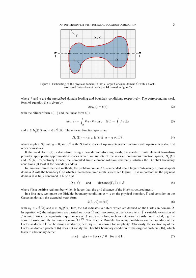
Figure 1. Embedding of the physical domain Ω into a larger Cartesian domain Ω with a block-structured finite element mesh (cut I-I is used in figure 2)

where f and g are the prescribed domain loading and boundary conditions, respectively. The corresponding weakform of equation (1) is given by

a(u, v) = `(v) (2)

with the bilinear form a(·, ·) and the linear form `(·)

a(u, v) =∫

Ω

∇u · ∇v dx , `(v) =∫

Ω

f v dx (3)

and u ∈ H1g (Ω) and v ∈ H1

0 (Ω). The relevant function spaces are

H1g (Ω) = u ∈ H1(Ω) |u = g on Γ , (4)

which implies H10 with g = 0, and H1 is the Sobolev space of square-integrable functions with square-integrable first

order derivatives.If the weak form (2) is discretized using a boundary-conforming mesh, the standard finite element formalism

provides appropriate approximation spaces which are subsets of the relevant continuous function spaces, H1g (Ω)

and H10 (Ω), respectively. Hence, the computed finite element solution inherently satisfies the Dirichlet boundary

conditions (at least at the boundary nodes).In immersed finite element methods, the problem domain Ω is embedded into a larger Cartesian (i.e., box-shaped)

domain Ω with the boundary Γ on which a block-structured mesh is used, see Figure 1. It is important that the physicaldomain Ω is fully contained in Ω so that

Ω ⊂ Ω and distance(Γ, Γ) > δ , (5)

where δ is a positive real number which is larger than the grid distance of the block-structured mesh.In a first step, we ignore the Dirichlet boundary conditions u = g on the physical boundary Γ and consider on the

Cartesian domain the extended weak forma(u1, v) = ˆ(v) (6)

with u1 ∈ H10 (Ω) and v ∈ H1

0 (Ω). Here, the hat indicates variables which are defined on the Cartesian domain Ω.In equation (6) the integrations are carried out over Ω and, moreover, as the source term f a suitable extension off is used. Since the regularity requirements on f are usually low, such an extension is easily constructed, e.g., byzero extension into the fictitious domain Ω \ Ω. Note that the Dirichlet boundary conditions on the boundary of theCartesian domain Γ can be chosen arbitrarily; here, u1 = 0 is chosen for simplicity. Obviously, the solution u1 of theCartesian domain problem (6) does not satisfy the Dirichlet boundary condition of the original problem (1b), whichleads to a boundary defect

h(x) = g(x)− u1(x) 6= 0 for x ∈ Γ . (7)


Γ ΓΓ ΓΩ

g g

u1

u2

u = u1 + u2

g g

h h

u1|Γ u1|Γ

(a)

(b)

(c)

(d)

Figure 2. Components of the solution along the cut I-I shown in figure 1: (a) boundary condition u = g on the physical boundaryΓ, (b) solution u1 of the Cartesian domain problem, (c) corrector u2 with defect h = g − u1|Γ and (d) final solution u

To enforce the Dirichlet boundary conditions of the original problem (1) we consider an auxiliary homogeneousboundary value problem on the physical domain Ω with

−(∇2u2)(x) = 0 for x ∈ Ωu2(x) = h(x) for x ∈ Γ .

(8)

The solution u of the original problem can now be recovered as the sum of the restriction of the Cartesian domainsolution u1 to the original (physical) domain Ω and the corrector u2

u = (u1)|Ω + u2 = u1 + u2 . (9)

In fact, the components u1 and u2 can be viewed as a combination of a particular and the corresponding homogeneoussolution of the original problem.

It remains to specify the discretization method for the auxiliary boundary value problem (8). This problem ishomogeneous but inherits the geometric complexity of the physical domain Ω. Staying with a classical finite elementapproach, the difficulty of constructing suitable approximation spaces for the original problem would be deferred tothis auxiliary problem. Therefore, we use an integral equation method for computing u2. The advantage of this choiceis that only a surface triangulation is needed for the discretization of the corresponding integral equation.

In figure 2, the section along the cut I-I shown in figure 1 is depicted. With this illustration at hand, the presentedsolution method consists of the following steps:

1. compute the solution u1 of the Cartesian domain problem (6) using a block-structured grid and the finiteelement method,

2. evaluate the boundary defect h along the physical boundary according to equation (7),3. compute the corrector u2 as the solution of the auxiliary problem (8) using an integral equation formulation,4. compute the final solution u as the superposition of the restriction of u1 to the physical domain Ω and the

corrector u2.

2.2. Finite element solution u1

Due to the extension Ω → Ω, it is straightforward to construct suitable approximations of the solution space H10 (Ω).

In particular, the choice of a Cartesian domain for Ω enables to use a simple block-structured mesh. The corresponding


trial functions ϕI are the piecewise polynomials on the elements associated with the grid nodes in the interior of Ω,which span the subspace

V h = spanϕI ⊂ H10 (Ω) . (10)

Then, the finite element approximation is of the form

u1(x) ≈ uh1 (x) =

N1∑I=1

ϕI(x)u1,I , (11)

where N1 = dim(V h) is the dimension of the finite element space V h. The subsequent steps in computing the finiteelement solution u1 are the same as in standard finite elements and can be found in any finite element textbook.

2.3. Integral equation correction u2

The solution u2 of the auxiliary homogeneous boundary value problem (8) can be represented by means of a singlelayer potential

u2(x) =∫

Γ

U∗(x− y)q(y) dsy , x ∈ Ω , (12)

where U∗(x− y) is the fundamental solution of the Laplace operator

U∗(x− y) = − 12π

log |x− y| . (13)

The function q : Γ→ R is the, yet unknown, surface density which is determined from

h(x) =∫

Γ

U∗(x− y)q(y) dsy , x ∈ Γ . (14)

This integral equation is obtained by taking the limit Ω 3 x → x ∈ Γ in equation (12) and using the Dirichletboundary condition of problem (8). Note that the integration in equation (14) has to be understood in an impropersense, because the integrand has a weak singularity as y approaches x (see, e.g., [16]). To obtain an approximation tou2 using equation (12), first a suitable discretization of the integral equation (14) has to be introduced. To this end thesurface density q and the boundary value h are approximated with

q(x) ≈∑

J

ψJ(x)qJ and h(x) ≈∑K

χK(x)hK , (15)

where ψJ and χK are the shape functions. Owing to the mapping properties of the boundary integral operator inequation (14), it is possible to use piecewise constant polynomials for the trial functions ψJ and piecewise linearcontinuous polynomials for the interpolation functions χK , see [8, 10, 16]. For higher order approximations it isimportant that the trial functions ψJ allow for discontinuous source distributions at domain corners.

To solve integral equation (14) a collocation method is used. Hence, at each collocation point x∗L ∈ Γ on thephysical boundary the condition to be satisfied is∑

J

∫Γ

U∗(x∗L − y)ψJ(y) dsy qJ =∑K

hKχK(x∗L) . (16)

Choosing sufficiently many and well-placed collocation points x∗L, equation (16) yields a system of linear equationsfor determining the unknown source densities qJ . Note that the related matrix coefficients are in general non-zero forall combinations of ψJ and x∗L so that the resulting system matrix is fully populated. Once, the source densities qJhave been computed, the approximate correction is computed with the single layer potential at any point x inside thephysical domain Ω:

uh2 (x) =

∑J

∫Γ

U∗(x− y)ψJ(y) dsyqJ . (17)

To avoid the rather involved analytical computation of the integrals in equations (16) and (17), numerical quadratureis used. The application of quadrature rules to these integrals is not straightforward due to the divergent behaviour of


the integral kernels as the integration variable y approaches the collocation point x∗L. In the integration in equation (16)two cases can be distinguished: (i) singular integration if x∗L is in the support of ψJ(y) or (ii) regular integration ifthis is not the case. In the singular case, first a coordinate transformation is applied which removes the singularity. Inthe two-dimensional implementation presented in this work the semi-sigmoidal transform suggested by Johnston [17]is used. Although there is no distinct singularity in the regular case, it is possible that the point x∗L is very closeto the support of ψJ(y). For this so-called quasi-singular integration, an adaptive quadrature rule is used whichrecursively subdivides the integration interval according to some heuristic rule depending on the size of this intervaland its minimal distance to the collocation point. For further details on this approach see [18]. Note that the adaptiveintegration is also well suited for evaluating the integrals appearing in equation (17).

2.4. Implicit boundary representation

In the proposed method, it is necessary to determine the position of the finite element nodes of the structured meshwith respect to the physical domain boundary Γ. It is, for instance, necessary to know if a node is located inside oroutside the physical domain Ω. To this end, a level set representation of the domain surface Γ in form of a signeddistance field φ(x, Γ) is used, see [19],

φ(x, Γ) =

distance(x,Γ) if x ∈ Ω0 if x ∈ Γ−distance(x,Γ) otherwise .

(18)

This functions yields the distance between the point x and the domain surface Γ and is positive if x is inside Ω andnegative else. The domain surface Γ coincides with the zero contour of the level set function φ(x, Γ). In this work,the signed distance function is computed using the highly efficient closest point algorithm given in [20].

2.5. Illustrative example

As an illustrative example we consider the Poisson equation

−∇2u = 1 for x ∈ Ω , u = 0 for x ∈ Γ (19)

on a circular domain of radius 0.5, i.e., Ω = x ∈ R2 | |x| < 0.5. The analytical solution of this equation is

u(x) =116

(1− 4|x|2

). (20)

The Cartesian domain is chosen to be Ω = (−0.6, 0.6)× (−0.6, 0.6) which is discretized with four-node rectangularfinite elements. The surface is discretized with piecewise linear functions for the boundary defect h and piecewiseconstant functions for the surface density q. This example is solved using different mesh combinations which aredenoted by the numbers NFE/NIE . NFE represents the number of finite element nodes in each direction (resultingin N2

FE total nodes). NIE refers to the number of boundary segments. Figure 3 shows a representative numericalsolution and its finite element and integral equation components with a mesh combination 41/40.

The error in the solution e(x) = |u(x) − uh(x)| is computed with the known analytical solution (20). The errordistribution along the diagonal x1 = x2 from the centre of the circle to its boundary is plotted in figure 4 for differentmesh sizes. The coarsest mesh combination is 41/40 and three finer meshes are obtained by quadrisecting the bilinearfinite elements and bisecting the boundary elements. Clearly, the error decreases in overall magnitude for decreasingmesh sizes. Moreover, one can detect from the oscillatory pattern of the error curves (which is most pronounced for thefinest mesh), the higher accuracy when boundary segments pass through superconvergent points of the finite elementmesh. On the other hand, the results appear to be less accurate for points closer to the surface Γ. This is explained bythe loss of accuracy in evaluating the single layer potential (12) when the evaluation point gets closer to the integrationrange. Hence, this is an artifact of post-processing and, notably, it disappears with decreasing mesh size.


(a) Mesh and domain boundary (b) u1

(c) u2 (d) u = u1 + u2

Figure 3. Solution of the Poisson equation on a circular domain: (a) Cartesian domain with the structured mesh and thecircle describing the domain boundary, (b) finite element solution u1 on the Cartesian domain, (c) integral equation

solution u2 and (d) the solution u = (u1)|Ω + u2 of the original problem

1e-07

1e-06

1e-05

1e-04

1e-03

0 0.1 0.2 0.3 0.4 0.5

|u –

uh|

radial coordinate |x|

41/4081/80

161/160321/320

Figure 4. Error in the solution along the diagonal (x1 = x2) of the circle for four different meshes


3. VISCOUS INCOMPRESSIBLE FLOW

3.1. Navier-Stokes equations

Viscous incompressible fluid flow is described by the Navier-Stokes equations which can be expressed in the stress-divergence form as

ρDu

Dt−∇ · σ(u, p) = f , ∇ · u = 0 , (21)

where u = u(x, t) denotes the velocity vector and ρ the mass density. The Newtonian fluid stress tensor σ is definedas

σ(u, p) = −pI + µ[∇u + (∇u)>] . (22)

where p = p(x, t) is the hydrostatic pressure, I the identity tensor, and µ is the dynamic viscosity. The first equationin (21) is the momentum balance with the total time derivative

Du

Dt=∂u

∂t+ (u · ∇)u . (23)

The second equation in (21) is the so-called incompressibility condition∇·u = 0, which represents the mass balancefor an incompressible fluid with constant mass density. Inserting the expression for the stress tensor (22) and the totaltime derivative (23) into the momentum balance equation (21) and making use of the incompressibility condition,yields the initial boundary value problem for viscous incompressible flow

∂u

∂t+ (u · ∇)u− ν∇2u +

1ρ∇p =

1ρf , ∇ · u = 0 for x ∈ Ω

u = g for x ∈ Γu(·, t = 0) = 0 for x ∈ Ω

(24)

with the prescribed boundary velocities g and the kinematic viscosity ν = µ/ρ.To derive the semi-discrete Navier-Stokes equations, the time variable is subdivided into subintervals t0 = 0 <

t1 < · · · < tn < tn+1. Furthermore, the shorthand notation un = uh(·, tn), pn = ph(·, tn), fn = f(·, tn) and∆t = tn+1 − tn is introduced. The time discretization of the Navier-Stokes equations (24) with the backward Eulermethod gives the nonlinear recurrence relation

1∆t

un+1 + (un+1 · ∇)un+1 − ν∇2un+1 +1ρ∇pn+1 =

1∆t

un +1ρfn+1 (25)

subject to ∇ · un+1 = 0. If the solutions un and pn at time tn are known, the solution at tn+1 can be computed witha fixed point iteration (see, e.g., [21])

1∆t

u(k+1) + (u(k) · ∇)u(k+1) − ν∇2u(k+1) +1ρ∇p(k+1) =

1∆t

un +1ρfn+1

∇ · u(k+1) = 0 ,(26)

where some of the time indices have been dropped and the superscripts (·)(k) refer to the k-th iterate. This iterationscheme is initialised with the predictor u(k) = un and converges to the new solution un+1 = u(k+1) at tn+1.Importantly, equation (26) is linear in the unknowns u(k+1) and p(k+1). Therefore, these unknowns can again bewritten as the superposition of a finite element solution on a Cartesian domain u1 and integral equation correction u2

u(k+1) = u1 + u2 . (27)

There is a slight abuse of notation here since the indices in u1 and u2 do not refer to time. After introducing thesedecompositions into the fixed point iteration equation (26) two linear system of equations are obtained for computingu1 and u2.


3.2. Finite element solution (u1, p1)

The solution pair (u1, p1) is obtained by solving the following linear equation system using a finite element method

1∆t

u1 + (u(k) · ∇)u1 − ν∇2u1 +1ρ∇p1 =

1∆t

un +1ρfn+1 − (u(k) · ∇)u2 for x ∈ Ω

∇ · u1 = 0 for x ∈ Ω

u1 = 0 for x ∈ Γ

(28)

where Ω is the Cartesian domain and Γ is its boundary. Further, recall that u1 and p1 denote the extensions of u1 andp1 from the physical domain to the Cartesian domain, respectively. The specification of these extensions is deferredto section 3.4. In equation (28), note the appearance of the unknown integral equation correction u2 on the right handside. Since the advection term has to be treated in an explicit manner for the boundary integral correction part (theoperator would otherwise be inhomogeneous), it has to be handled as a body force in the finite element solution stepin order to maintain consistency.

The finite element discretization of the equation (28) requires a weak form which reads

1∆t

(u1, v)Ω + c(u(k), u1, v) + a(u1, v)− b(p1, v) = ˜(v)

b(γ, u1) = 0(29)

with the trial functions (u1, p1) ∈ [H10 (Ω)]d × L0

2(Ω) and the test functions (v, γ) ∈ [H10 (Ω)]d × L0

2(Ω). Theabbreviations in equation (29) are as follows

a(u1, v) =∫

Ω

ν∇u1 : ∇v dx ,

c(w, u1, v) =∫

Ω

[(w · ∇)u1] · v dx ,

b(γ, v) =∫

Ω

1ργ(∇ · v) dx ,

˜(v) =1ρ

∫Ω

fn+1 · v dx +1

∆t(un, v)Ω − c(u

(k), u(k)2 , v) ,

(30)

where (a, b)Ω =∫Ω

a · bdx is the L2-product, and L02(Ω) = γ ∈ L2 |

∫Ωγ dx = 0 is the space of all square-

integrable functions whose mean vanishes. This special space is introduced because the pressure is only known upto an arbitrary constant for the Navier-Stokes equations with only Dirichlet boundary conditions. In order to ensurethis vanishing mean and thus guarantee solvability, the second equation in (29) is actually augmented by the termd(p1, γ) = (p, 1)Ω(γ, 1)Ω = 0. As well known, the finite element discretization of the variational statement (29)has to be performed with care in order to avoid stability problems (see, e.g., [22]). Here, the Taylor-Hood element ischosen which is inherently LBB-stable [22].

3.3. Integral equation correction (u2, p2)

The correction component u2 of the solution is obtained from the linear homogeneous boundary value problemρ

∆tu2 − µ∇2u2 +∇p2 = 0 , ∇ · u2 = 0 for x ∈ Ω

u2 = h for x ∈ Γ(31)

with the boundary defect h = g − (u1)|Γ. Recall that g is the prescribed velocity boundary condition of the originalproblem and u1 is the finite element solution on the Cartesian domain. Equation (31) is known as the Brinkman ormodified Stokes problem and the corresponding fundamental solution is given in the appendix in equation (50). Usingthe fundamental solution for the velocities, u2 can be represented with the single layer potential

u2(x) =∫

Γ

U∗(x− y)q(y) dsy , x ∈ Ω , (32)


where q is the unknown vectorial surface density, which is determined from the integral equation

h(x) =∫

Γ

U∗(x− y)q(y) dsy , x ∈ Γ . (33)

The discretization and solution of this equation is carried out along the lines of the scalar problem introduced insection 2.3.

The pressure distribution is computed with the pressure single layer potential

p2(x) =∫

Γ

P ∗(x− y)q(y) dsy , x ∈ Ω (34)

using the surface density q determined by equation (33). For Navier-Stokes equations with pure Dirichlet boundaryconditions, the pressure distribution p can only be determined up to a constant c. The same is true for the surfacetraction t = σ(u, p) · n, where n is the unit surface normal. According to the stress definition (22), replacing p bysome shifted value p + c alters the traction by −cn. This deficiency carries over to the single layer potential (32),see [16] for mathematical details in case of the Stokes system. As a result, the vector field n is an eigensolution of thesingle layer integral equation with corresponding zero eigenvalue, or formally,∫

Γ

U∗(x− y)n dsy = 0 . (35)

Therefore, the discretized integral equations are ill-conditioned. In fact, the corresponding system matrix has a zeroeigenvalue and the associated eigenvector is a discrete representation of the surface normal field n. In order to resolvethis problem, the stabilisation presented in [23] for the Galerkin boundary element method is adapted to the usedcollocation method. This stabilisation is carried out by adding to each d× d-matrix block of the system matrix (here,d = 2 for two-dimensional problems), the matrix block of the form

NLJ =1µ

n(x∗L)⊗∫

Γ

n(y)ψJ(y) dsy , (36)

which corresponds to the collocation point x∗L and the shape function ψJ . Note that this procedure is equivalent to adeflation of the corresponding eigenvalues in matrix analysis [24]. The factor of 1/µ in equation (36) is introduced toensure that the extra matrix entries are of similar magnitude as the original matrix entries stemming from equation (16).In case of a multiply connected boundary surface, this stabilisation technique has to be generalised accordingly,see [23] for details.

All the expressions given so far in this section refer to the unsteady flow case. Nevertheless, the steady statelimit is recovered by neglecting the expressions with the partial time derivatives from the governing and subsequentequations. The only noteworthy change involves the integral equation solution which reduces to a Stokes equationwith the corresponding stokeslet as the fundamental solution (see appendix, equation (48)).

3.4. Extrapolation of the physical domain variables

In order to ensure the convergence and robustness of the proposed algorithm, special care needs to be taken inextending physical domain variables into the fictitious domain. In particular, in the iteration (28) for computing thefinite element solution u1, the integral equation solution u2 over the entire Cartesian domain is required. However,the integral equation solution outside of the physical domain is not defined and is not of physical relevance. Thus, itcan be chosen in Ω \ Ω based on ease of numerical implementation.

To motivate our particular choice of the extension operator used, consider the situation depicted in figure 5. Thefinite element nodes are represented by squares and the nodes of the surface mesh by circles. Moreover, the nodes xI

and xI+1 are located in the physical domain Ω and the nodes xM and xM+1 are in the fictitious domain Ω \ Ω. Forthe nodes inside the physical domain, the finite element solution u1 as well as the integral equation solution u2 areavailable and their superposition yields the solution u = u1 + u2. In contrast, for the nodes in the fictitious domainonly the finite element solution is available, but not the integral equation solution. In our implementation the velocitiesu2 for the nodes outside physical domain Ω are determined by constant extrapolation from the closest point on thedomain boundary (indicated by the dotted lines in figure 5). The function value at this point is given by evaluating theboundary element approximation (15). In order to obtain the closest point, the closest point algorithm of Mauch [20]is used, which delivers the necessary quantities with optimal computational complexity.


ΓΩ

Ω \ Ω

xJ

xJ−1

xJ+1

xI xI+1

xM xM+1

Figure 5. Quadrilateral finite element mesh traversed by a surface mesh

3.5. Evaluation of the boundary defect

Another remark concerns the computation of the boundary defect h. For flow problems, the finite element velocitiesu1 are interpolated with piecewise bi-quadratic polynomials and the defect h in the velocities is interpolated withpiecewise linear functions. For such a combination, the interpolation of the nodal defect values using the finite elementshape functions with

hK = g(xK)− uh1 (xK) = g(xK)−

∑I

ϕI(xK)u1,I (37)

does not lead to satisfactory results. This equation contains the difference between a linear polynomial (approximationof g) and a polynomial with up to fourth order terms. In order to mitigate this mismatch, the interpolation shapefunctions ϕI in equation (37) are replaced with piecewise linear shape functions.

3.6. Fluid traction

In some applications, in addition to the velocity-pressure pair (u, p) also the traction field t = σ(u, p) · n on thesurface Γ needs to be computed. Since the integral equation solution pair (u2, p2) is not available outside the physicaldomain Ω, the contribution of the integral equation solution is computed using

t2(x) = (Cq)(x) +∫

Γ

T ∗(x− y)q(y) dsy , (38)

which is commonly referred to as the adjoint double layer potential. This expression is obtained by inserting the singlelayer potentials for the velocity (12) and pressure (34) into the definition of the fluid stress tensor (22), moving theevaluation point to the surface and multiplying the result with the surface normal vector n(x). This yields the newintegral kernel T ∗ and the jump term Cq due to the limiting process [10, 16]. If the evaluation point x is positionedon a smooth part of the boundary Γ, the jump term is simply (Cq)(x) = 1

2q(x). To ensure the sufficient smoothnessof the adjoint double layer potential (38), it is evaluated inside the boundary elements and not at their vertices. Notethat for the applications presented in this work, the integral kernel T ∗ remains weakly singular, whereas, for instance,in the case of linear elasticity the integration in (38) has to be carried out in the sense of a Cauchy principal value (see,e.g. [16]). An explicit expression of T ∗ can be found in [25].

3.7. Examples

3.7.1. Circular Couette flow. As a first example for the Navier-Stokes equations, the circular Couette flow isconsidered (see, e.g., [26]). This flow occurs between two coaxial cylindrical surfaces Γ1 and Γ2 with radii r1 andr2 which rotate with constant angular velocities ω1 and ω2, respectively. The stationary flow pattern is axisymmetricand, hence, is best described in polar coordinates (r, φ). The analytical solution for the velocity and pressure is

ur = 0 , uφ(r) = Ar +B

r, p(r) =

A2

2r2 + 2AB log r − B2

2r2+ C (39)


2

4

6

8

10

0.5 0.6 0.7 0.8 0.9 1

vel

oci

ty u

φ

radial coordinate r

-15

-10

-5

0

5

10

0.5 0.6 0.7 0.8 0.9 1

pre

ssure

p

radial coordinate r

Figure 6. Tangential velocity uφ (left) and the pressure p (right) across the radius; the solid lines represent theanalytical solution according to equation (39) and the crosses the computed values

with

A =ω1r

21 − ω2r

22

r21 − r22, B =

(ω1 − ω2)r21r22

r22 − r21. (40)

The pressure is defined up to an arbitrary constant C. The torque on the cylinders is T = ±4πµB, where the plussign refers to the outer and the minus sign to the inner cylinder. For the numerical computations, a physical domain Ωwith an internal radius r1 = 0.5 and an external radius r2 = 1 is chosen. The internal cylinder rotates with the angularvelocity ω1 = 0.1 and the external with ω2 = 10, which give, according to equation (40), A = 13.3 and B = −3.3.The Cartesian domain is a square with Ω = (−1.2, 1.2)× (−1.2, 1.2) and is discretized with 7 569 Q2-Q1 rectangles.The surfaces of the cylinders are discretized with 320 (outer cylinder) and 160 (inner cylinder) line elements witha piecewise constant approximation for the surface density q and continuous piecewise linear interpolation of theDirichlet datum h. In the numerical computations the viscosity of the fluid is chosen as µ = 0.1 and its density asρ = 1. Note that the analytical solution of the circular Couette flow is independent of the viscosity and density.

In Figure 6, the analytical and numerical solutions of the tangential velocity uφ and the pressure p across the radiusare compared. The very good agreement between the analytical and numerical solutions is evident. A closer lookreveals only a slight deviation of the pressure solution towards the boundaries. The constant C in equation (39)is adjusted such that the numerical and analytical solutions agree at the midpoint, i.e., ph(rm) = p(rm) forrm = (r1 + r2)/2.

In addition, the torque T acting on the two cylinders is computed with

Ti =∫

Γi

(x− x0)× [σ(u, p) · n] dsx (41)

where the origin x0 is chosen as the centre of the rotation and the index i = 1, 2 refers to the outer or inner surface,respectively. The vector product ’×’ in equation (41) is to be understood in the usual vectorial sense with the resultingtorque vector pointing in the third coordinate direction. The temporal change of the torque magnitudes is given infigure 7, where one can clearly observe how they converge in the course of time. The exact stationary solution is givenas the solid line in the same figure. The relative numerical error in the computed torques is given in table I. Here, thenumerical solution of the steady problem is provided in addition to the unsteady solution. In both cases, the resultsfor the outer cylinder are less accurate than the results for the inner cylinder, which can be attributed to the relativecoarseness of the finite element mesh for the outer cylinder in comparison to the inner cylinder.

3.7.2. Driven cavity. The next verification example is the driven cavity which has been extensively used as a test casein literature. The physical fluid domain is a unit square Ω = (−0.5, 0.5)× (−0.5, 0.5) with a prescribed unit velocityalong its top boundary and no-slip boundary along the remaining boundaries. The fluid has a density of ρ = 1 so thatthe Reynolds number is controlled by Re = 1/µ. The Cartesian domain is a square Ω = (−0.6, 0.6) × (−0.6, 0.6),which is discretized with (NFE − 1)2/4 finite elements with Q2-Q1 interpolation. The surface discretization


0

2

4

6

8

10

0 0.5 1 1.5 2 2.5 3

torq

ue T

time t

outerinner

exact limit

Figure 7. Magnitude of the torque against time for the outer and inner cylinder and the exact stationary solution

steady unsteady exact

inner 4.158 (0.27%) 4.179 (0.74%) 4.147outer 4.264 (2.8%) 4.311 (4.0%) 4.147

Table I. Magnitudes and relative errors of the torques on the cylinders

consists of 4NIE line elements with constant shape functions. In all computations the convergence criterion is|u(k+1) − u(k)| < 10−5.

In figure 8, the contour lines for the velocity magnitude and the pressure are plotted for Re = 400. Additionally,the streamlines computed from the velocity field are also given in figure 8. This flow field is obtained by a steady stateanalysis with NFE = 161 and NIE = 160, i.e., 6400 quadrilateral finite elements and 640 line elements. The keyfeatures of the driven cavity flow at Re = 400 are a core vortex and two smaller vortices at the bottom corners, whichare all well reproduced by the computation.

(a) Velocity magnitude (b) Pressure (c) Streamlines

Figure 8. Contour lines of velocity magnitude |u|, pressure p and streamlines for Re = 400

This example is subjected to a more systematic mesh convergence study using the reference solutions of Ghia etal. [27] for Reynolds numbers 100, 400 and 1000. In a first set of computations, the mesh parameters NFE and NIE

are simultaneously varied. Figure 9 shows the u1 component of the computed velocities along the x2-axis and theiru2 component along the x1-axis for the considered three Reynolds numbers and three different mesh sizes togetherwith the reference solutions. The plotted data were obtained with a steady state analysis. In each case, there is a good


agreement between the reference and numerical solutions and in most cases already relatively coarse meshes give verygood results. Note that for higher Reynolds numbers, the used element sizes are always a step smaller in line withhigher resolution requirements.

In a second set of computations, the mesh parametersNFE andNIE are independently varied for the problem withReynolds number 400. In figure 10, the finite element mesh stays the same with NFE = 41 and for the surface meshNIE is 20, 40 or 80. Figure 11 shows the results for the opposite case, where the surface mesh stays the same withNIE = 40 and for the finite element mesh NFE is 21, 41 and 81. In the first case, where the surface mesh is refinedand the finite element mesh size is fixed, the numerical solution converges to the reference result with successivemesh refinement. In the second case, where the finite mesh is refined and the surface mesh size is fixed, the numericalsolution slightly deteriorates with successive mesh refinement. From these numerical studies can be concluded thatthe characteristic element size of the finite element mesh and the surface mesh have to be comparable in order toachieve maximum accuracy.

Next, in order to investigate how the relative placement of the surface mesh with respect to the structured finiteelement mesh influences the results, the physical domain is rotated by an angle of 30 and 45 degrees. The meshparameter of the surface mesh is NIE = 80. In order to accommodate for the rotated surface, the Cartesian domain isenlarged to Ω = (−0.8, 0.8) × (−0.8, 0.8). Its mesh parameter is NFE = 107, which is comparable to NFE = 81for the smaller domain used previously. In figure 12, the velocity profiles for Re = 400 are given, which clearly showthat the numerical results are only slightly influenced by the domain rotation.

4. FLUID-RIGID BODY INTERACTION

4.1. Problem formulation

A key advantage of the proposed discretization method is that the finite element mesh on the Cartesian domain does notdepend on the location of the immersed domain boundaries. This is particularly appealing for applications with movingboundaries. As an example for such an application, the settling of a particle in a closed tank filled with a viscous fluidis considered. Finite element simulations of particle settling with adaptive remeshing have been presented, amongstothers, in [28] and [29].

The considered setup is depicted in figure 13, where a circular particle P is located at the position (x1, x2) =(X1, X2) with an orientation angle ϑwith respect to the horizontal axis. The tank ΩT with boundary ΓT is rectangularand has the dimensions W × H . The velocity of the particle is U = (U1, U2) and it rotates around its centreX = (X1, X2) with the angular velocity ω = ϑ. The gravity field g = (0,−g) acts vertically downwards. If themass density of the particle is larger than the fluid density, its weight will accelerate it downwards. At the same time,the fluid in the tank exerts a drag force on the particle which depends on the fluid flow in the tank.

This coupled problem is described by Newton’s law for the particle and the Navier-Stokes equations forincompressible viscous fluid flow (21). The boundary conditions of the fluid problem are no-slip conditions at thetank walls and at the particle surface

u = 0 x ∈ ΓT (42)u = U + ω × (x−X) x ∈ ∂P (t) , (43)

wherein the vector product × has to be understood in a three-dimensional sense. Equation (43) emphasises that thelocation of the boundary ∂P , i.e., the surface of the particle, is a function of time. The fluid problem thus consistsof the Navier-Stokes equations (21) with gravity as a body force and equations (42) and (43) as velocity boundaryconditions. The fluid is assumed to be initially at rest so that the initial condition is u0 = 0.

The motion of the particle itself is governed by Newton’s law, i.e.,

mdU

dt= F ,

dX

dt= U , (44a)

Jdωdt

= T ,dϑdt

= ω . (44b)

The first equation (44a) describes the translational motion and m denotes the particle mass. The rotational motion isdescribed by equation (44b), where J refers to the polar moment of inertia.


-0.4

-0.2

0

0.2

0.4

0.6

0.8

1

0 0.2 0.4 0.6 0.8 1

vel

oci

ty u

1

coordinate x2

Ghia et al.11/1021/2041/40

-0.3

-0.2

-0.1

0

0.1

0.2

0 0.2 0.4 0.6 0.8 1

vel

oci

ty u

2

coordinate x1

Ghia et al.11/1021/2041/40

(a) Re = 100

-0.4

-0.2

0

0.2

0.4

0.6

0.8

1

0 0.2 0.4 0.6 0.8 1

vel

oci

ty u

1

coordinate x2

Ghia et al.21/2041/4081/80

-0.6

-0.4

-0.2

0

0.2

0.4

0 0.2 0.4 0.6 0.8 1

vel

oci

ty u

2

coordinate x1

Ghia et al.21/2041/4081/80

(b) Re = 400

-0.4

-0.2

0

0.2

0.4

0.6

0.8

1

0 0.2 0.4 0.6 0.8 1

vel

oci

ty u

1

coordinate x2

Ghia et al.41/4081/80

161/160

-0.6

-0.4

-0.2

0

0.2

0.4

0 0.2 0.4 0.6 0.8 1

vel

oci

ty u

2

coordinate x1

Ghia et al.41/4081/80

161/160

(c) Re = 1000

Figure 9. Velocity profiles of the driven cavity for Reynolds numbers 100, 400 and 1000; the number pairs NFE/NIE

in the legends refer to the mesh parameters (see text)


-0.4

-0.2

0

0.2

0.4

0.6

0.8

1

0 0.2 0.4 0.6 0.8 1

vel

oci

ty u

1

coordinate x2

Ghia et al.41/2041/4041/80

-0.6

-0.4

-0.2

0

0.2

0.4

0 0.2 0.4 0.6 0.8 1

vel

oci

ty u

2

coordinate x1

Ghia et al.41/2041/4041/80

Figure 10. Velocity profiles of the driven cavity for Re = 400 for fixed finite element mesh and successively refinedsurface meshes

-0.4

-0.2

0

0.2

0.4

0.6

0.8

1

0 0.2 0.4 0.6 0.8 1

vel

oci

ty u

1

coordinate x2

Ghia et al.21/4041/4081/40

-0.6

-0.4

-0.2

0

0.2

0.4

0 0.2 0.4 0.6 0.8 1

vel

oci

ty u

2

coordinate x1

Ghia et al.21/4041/4081/40

Figure 11. Velocity profiles of the driven cavity for Re = 400 for fixed surface mesh and successively refined finiteelement meshes

-0.4

-0.2

0

0.2

0.4

0.6

0.8

1

0 0.2 0.4 0.6 0.8 1

vel

oci

ty u

1

coordinate x2

Ghia et al.0°

30°

45°

-0.6

-0.4

-0.2

0

0.2

0.4

0 0.2 0.4 0.6 0.8 1

vel

oci

ty u

2

coordinate x1

Ghia et al.0°

30°

45°

Figure 12. Velocity profiles of the driven cavity for Re = 400 for different rotations of the surface


It remains to specify the force F and the torque T which act on the particle. The force and the torque on the particlewith the surface normal n are given by

F = mg −∫

∂P (t)

σ(u, p) · n ds and T = −∫

∂P (t)

(x−X)× [σ(u, p) · n] ds . (45)

Note that the minus signs appear due to the orientation of the normal vector n which points by definition to the insideof the particle (or, outside of the fluid).

4.2. Coupling algorithm

The solution strategy used in this work is the semi-implicit predictor-corrector algorithm introduced by Hu et al. [28].It is assumed that the solution of the fluid-particle system is known at the current time step t = tn. Hence, thequantities Xn, ϑn, Un, ωn (i.e., the state of the particle) and un, pn (i.e., the state of the fluid) are known. Thenthe implicit iteration loop within each time step begins with the following predictor values for the particle force andtorque

F (0) = F (un, pn) and T (0) = T (un, pn) (46)

The subsequent nonlinear iterations consist of the following substeps:

1. Compute particle velocities U (k+1) = Un + α(∆t/m)F (k) and ω(k+1) = ωn + α(∆t/J)T (k).2. Solve the fluid problem for velocity u(k+1) and pressure p(k+1) with boundary conditions according to (43)

using the immersed finite element method described in section 3.3. Compute the force F (k+1) and torque T (k+1) with equation (45) based on the current fluid state

(u(k+1), p(k+1)).4. Iterate k ← k + 1.

Once this nonlinear iteration is converged, the new particle velocities are assigned, i.e. Un+1 = U (k+1) andωn+1 = ω(k+1), and the new particle position and orientation is computed with a forward Euler step

Xn+1 = Xn + ∆tUn+1 and ϑn+1 = ϑ+ ∆tωn+1 . (47)

U1

U2

ω

g

x1

x2

W

H

Figure 13. Circular particle in a closed tank


As realised by Hu et al. [28], an under-relaxation improves the convergence of the coupling algorithm. Therefore, therelaxation parameter α is introduced in step 1, which is chosen with α = 0.4 as suggested in [28]. Note that step 2of the coupling algorithm still involves the solution of a fully nonlinear problem which requires sub-iterations. In thecomputations usually only two to three such sub-iterations are sufficient.

4.3. Example

Two sets of computations using the above described coupling algorithm are carried out. In the first set of computations,the particle is released from the symmetry axis of the tank. In the second set, the particle is released from anoff-centre position. All other parameters are identical for both computations. The closed tank occupies the regionΩT = (−0.05, 0.05) × (0, 0.5) and the particle is of circular shape with radius rp = 0.01. The fluid has unit densityρ = 1 and the particle is twice as heavy with ρp = 2. The gravitation constant is chosen simply as g = 10. Theviscosity of the fluid is chosen as µ = 0.001. Based on the terminal settling velocity of about |U2| = 0.155 (seefigure 15), the particle Reynolds number is Re = 2rρU2/µ ≈ 3.1, which is well below the values for which vortexshedding can be expected.

The Cartesian domain is chosen as Ω = (−0.06, 0.06) × (−0.01, 0.51) and is discretized with 45 × 197 = 8 865Q2-Q1 finite elements. The boundary surfaces of the particle ∂P and the tank ΓT are discretized with 80 and 240 lineelements, respectively, using constant shape functions for the surface density. The temporal discretization begins witha time step size of ∆t = 0.001 which is increased for the first ten time steps by ten percent in each step yielding a finalstep size of approximately ∆t = 0.0026. Since in the computation the particle is suddenly equipped with its excessweight, numerical instabilities are likely to occur at the beginning of the computation. Therefore, it is reasonable tobegin the computation with a smaller time step size. Numerical instabilities also occur when the particle gets close tothe bottom wall. This effect is a lot more pronounced for the particle which was released from an eccentric position.For this reason, the computation was stopped after 800 time steps at approximately t = 2.0 or X2 = 0.18.

In the first computation the particle is released at position X = (0, 0.475) and in the second computation atX = (−0.03, 0.475). In figure 14 the particle paths for both computations are shown with the tank being rotatedby 90 degrees. Whereas the centred particle simply falls straight down due to its own weight, the initially eccentricparticle also moves horizontally. A closer look at its motion at the beginning reveals that it moves slightly towards theleft wall before reversing the direction and heading for the centre line X1 = 0. It overshoots a little and then returnsto the centre.

-0.05

0

0.05

0.1 0.2 0.3 0.4 0.5

X1

X2

centered excentric

Figure 14. Particle paths (rotated by 90 degrees)

Figure 15 shows the vertical particle position, its settling velocity and the force acting on it against time. Clearly, inboth cases the particle reaches the same terminal settling velocity of approximately U2 ≈ −0.155. This steady statesituation corresponds to an equilibrium of the particle excess weight of Wp = πr2p(ρp − ρ)g ≈ 3.1416 · 10−3 andthe drag force FD on the particle. The particle excess weight is indicated with a dotted horizontal line in figure 15(c),which serves as an asymptote for the drag force in both cases. The pictures in figure 15 also indicate that the verticalmotion of the particle with the initially eccentric position deviates noticeably from the particle which is initiallycentred in the acceleration phase t < 0.8. Its downward acceleration is clearly inhibited by its vicinity to the wall andit lags behind in terms of its vertical position.

The sequence of snapshots in figure 16 show the streamlines and pressure contours in the fluid at time instants0.25, 0.5, 1.0, 1.5 and 2.0 for the eccentric particle. Similarly, figure 17 shows the vorticity isolines and the velocity


0.2

0.3

0.4

0.5

0 0.5 1 1.5 2

vert

ical posi

tion X

2

time t

centeredexcentric

(a) Vertical position

-0.15

-0.1

-0.05

0

0 0.5 1 1.5 2

ver

tica

l vel

oci

ty U

2

time t

centeredexcentric

(b) Settling velocity

-0.003

-0.002

-0.001

0 0.5 1 1.5 2

vertic

al fo

rce F

2

time t

centered

excentric

(c) Particle force

Figure 15. Vertical position and velocity of the particle and fluid force acting on the particle

magnitude contours at the same time instants.

5. CONCLUSION

We have presented a new immersed finite element method for computing problems with complex, time-dependentdomains. In common with other immersed discretization methods only a surface mesh of the domain is required.The discretization of the embedding Cartesian domain relies on a non-body-conforming structured mesh, which canbe easily generated without resorting to specialised mesh generation algorithms. A unique feature of the proposedmethod is that the solution of the original problem is computed as the superposition of a finite element and an integralequation solution. As a result, the conditioning of the discretized equations does not depend on the shape and numberof cut-elements (i.e., finite elements traversed by the boundary mesh).

In the finite element solution on the Cartesian domain, the consideration of the physical domain leads only toa modified forcing term. This is relevant for using any pre-existing fast solver packages for finite elements, sinceonly suitably chosen boundary forces need to be prescribed. Furthermore, the structured mesh on the Cartesiandomain facilitates the use of solvers based on Fourier transforms or multigrid methods (see [13]). There are alsowell-established fast integral equation solvers that can be used for solving the integral equations, which appear in theproposed method (see, e.g., [30]). In this regard, it is important that the integral equations in the proposed methodcorrespond to homogeneous boundary value problems so that no costly Newton potentials need to be evaluated.


(a) t = 0.25 (b) t = 0.50 (c) t = 1.00 (d) t = 1.50 (e) t = 2.00

Figure 16. Streamlines and pressure contours at different time instants (excentric settling, bottom of tank is truncated)

(a) t = 0.25 (b) t = 0.50 (c) t = 1.00 (d) t = 1.50 (e) t = 2.00

Figure 17. Vorticity isolines and velocity magnitude contours at different time instants (excentric settling, bottom oftank is truncated)


ACKNOWLEDGEMENT

The support of the EPSRC through grant # EP/G008531/1 is gratefully acknowledged.

APPENDIX

FUNDAMENTAL SOLUTIONS

In the following, the two-dimensional fundamental solutions used in this work are given for completeness. In these equationsthe integration point is denoted with y and the collocation or evaluation point with x and I denotes the 2 × 2-identity matrix.References for the given fundamental solutions are, amongst others, [25, 10, 16].

Stokes system. The fundamental solutions of the Stokes system −µ∇2u +∇p = f , ∇ · u = 0 are of the form

U∗(x− y) =1

4πµ

„− log |x− y|I +

(x− y)⊗ (x− y)

|x− y|2

«(48)

P ∗(x− y) = − 1

2π

x− y

|x− y|2 . (49)

Brinkman system. The Brinkman or modified Stokes system reads (ρ/∆t)−µ∇2u+∇p = f ,∇·u = 0. With the abbreviationz = |x− y|

pρ/(µ∆t), the fundamental solutions are

U∗(x− y) =1

2πµz2

ˆ`z K1(z) + z2 K0(z)− 1

´I

+`2− 2z K1(z)− z2 K0(z)

´ (x− y)⊗ (x− y)

|x− y|2

–(50)

P ∗(x− y) = − 1

2π

x− y

|x− y|2 . (51)

where K0(z) and K1(z) are the modified Bessel functions of the second kind. In the numerical computations K0(z) and K1(z)are replaced by their asymptotic expansions for very small (z < 10−6) or very large (z > 500) arguments.

REFERENCES

1. Glowinski R, Pan TW, Periaux J. A fictitious domain method for Dirichlet problem and applications. Computer Methods in Applied Mechanicsand Engineering 1994; 111:283–303.

2. Peskin C. The immersed boundary method. Acta Numerica 2002; 11:1–39.3. Fedkiw R, T A, Merriman B, Osher S. A non-oscillatory Eulerian approach to interfaces in multimaterial flows (the ghost fluid method).

Journal of Computational Physics 1999; 152:457–492.4. Mittal R, Iaccarino G. Immersed boundary methods. Annual Review of Fluid Mechanics 2005; 37:239–261.5. Sukumar N, Chopp D, Moes N, Belytschko T. Modeling holes and inclusions by level sets in the extended finite element method. Computer

Methods in Applied Mechanics and Engineering 2001; 190:6183–6200.6. Belytschko T, Parimi C, Moes N, Sukumar N, Usui S. Structured extended finite element methods for solids defined by implicit surfaces.

International Journal for Numerical Methods in Engineering 2003; 56:609–635.7. Hansbo A, Hansbo P. An unfitted finite element method, based on Nitsche’s method, for elliptic interface problems. Computer Methods in

Applied Mechanics and Engineering 2002; 191:5537–5552.8. Banerjee P, Butterfield R. Boundary element methods in engineering science. McGraw-Hill, 1981.9. Aliabadi M. The boundary element method; applications in solids and structures, vol. 2. John Wiley & Sons Ltd., 2002.

10. Steinbach O. Numerical Approximation Methods for Elliptic Boundary Value Problems. Springer, 2008.11. Jung M, Steinbach O. A finite element-boundary element algorithm for inhomogeneous boundary value problems. Computing 2002; 68:1–17.12. Mayo A. The fast solution of Poisson’s and the biharmonic equations on irregular regions. SIAM Journal on Numerical Analysis 1984;

21:285–299.13. Biros G, Ying L, Zorin D. A fast solver for the Stokes equations with distributed forces in complex geometries. Journal of Computational

Physics 2004; 193:317–348.14. Tornberg AK, Shelley MJ. Simulating the dynamics and interactions of flexible fibers in Stokes flows. Journal of Computational Physics

2004; 196:8–40.15. Veerapaneni S, Gueyffier D, Zorin D, Biros G. A boundary integral method for simulating the dynamics of inextensible vesicles suspended in

a viscous fluid in 2D. Journal of Computational Physics 2009; 228:2334–2353.16. Hsiao G, Wendland W. Boundary Integral Equations. Springer, 2008.


17. Johnston P. Semi-sigmoidal transformations for evaluating weakly singular boundary element integrals. International Journal for NumericalMethods in Engineering 2000; 47:1709–1730.

18. Ruberg T, Schanz M. An alternative collocation boundary element method for static and dynamic problems. Computational Mechanics 2009;44:247–261.

19. Cirak F, Deiterding R, Mauch S. Large-scale fluid-structure interaction simulation of viscoplastic and fracturing thin-shells subjected to shocksand detonations. Computers & Structures 2007; 85:1049–1065.

20. Mauch S. A fast algorithm for computing the closest point and distance transform. Technical Report, California Institute of Technology 2000.21. Gresho P, Sani R. Incompressible Flow and the Finite Element Method. 1998, John Wiley & Sons.22. Ern A, Guermond JL. Theory and Practice of Finite Elements. Springer, 2003.23. Reidinger B, Steinbach O. A symmetric boundary element method for the Stokes problem in multiple connected domains. Mathematical

Methods in the Applied Sciences 2002; 26:77–93.24. Golub G, van Loan C. Matrix Computations. Johns Hopkins University Press, 1996.25. Pozrikidis C. A practical guide to Boundary Element Methods with the Software Library BEMLIB. Chapman & Hall/CRC, 2002.26. Batchelor G. An Introduction to Fluid Dynamics. Cambridge University Press, 1967.27. Ghia U, Ghia K, Shin C. High-Re solutions for incompressible flow using the Navier-Stokes equations and a multigrid method. Journal of

Computational Physics 1982; 48:387–411.28. Hu H, Joseph D, Crochet M. Direct simulation of fluid particle motions. Theoretical and Computational Fluid Dynamics 1992; 3:285–306.29. Saksono P, Dettmer W, Peric D. An adaptive remeshing strategy for flows with moving boundaries and fluid-structure interaction. International

Journal for Numerical Methods in Engineering 2007; 71:1009–1050.30. Bebendorf M. Hierarchical Matrices — A Means to Efficiently Solve Elliptic Boundary Value Problems. Springer, 2008.

an immersed finite element method with integral equation correction · pdf file ·...

Documents