an implementation of the finite element method for the

An Implementation of the Finite Element Method for the Velocity-CurrentMagnetohydrodynamics Equations

by

K. Daniel Brauss

A dissertation submitted to the Graduate Faculty ofAuburn University

in partial fulfillment of therequirements for the Degree of

Doctor of Philosophy

Auburn, AlabamaAugust 2, 2014

Keywords: magnetohydrodynamics, finite element method, numerical solution

Copyright 2014 by K. Daniel Brauss

Approved by

A. J. Meir, Chair, Professor of Mathematics and StatisticsPaul G. Schmidt, Professor of Mathematics and Statistics

Yanzhao Cao, Professor of Mathematics and StatisticsDmitry Glotov, Professor of Mathematics and Statistics

Abstract

The aim of this research is to extend the numerical results in [78] of a velocity-current

magnetohydrodynamics formulation proposed by A.J. Meir and Paul G. Schmidt in [74]

for a stationary flow that models a conductive fluid in a bounded domain. A parallel fi-

nite element algorithm was successfully implemented on a high-performance computing,

distributed-memory architecture at the Alabama Supercomputer Center (ASC) using the

freely available, open-source academic and government libraries deal.ii, p4est and Trilinos.

Extending the work of Elman, Silvester and Wathen [37] for the Navier-Stokes equations,

a Schur complement preconditioner was developed for the current saddle-point problem to

successfully utilize the iterative Krylov subspace solver GMRES (generalized minimal resid-

ual method) and solve large linear systems of equations arising from mesh refinement. To

simplify and lower operation costs in forming the preconditioner, spectral equivalence was

established between the Schur complement and a mass matrix. The resulting C++ code was

tested succesfully on problems from [78] with similar results.

ii

Acknowledgments

I have to thank God for the opportunity to continue my studies here at Auburn University. I

have to thank my wife Minvera Rosario Brauss Blanco for her unwavering support. Without

my wife, I would not have made it this far. Thank you Rose. I thank Eliana Catherine

Brauss, my daughter, for being here and filling our lives. I thank all of my family for their

support with all that we do. I thank all of my teachers for the passion that they have given

to me. I thank Dr. A. J. Meir for his much appreciated support, patience and guidance as

my Ph.D. advisor. Dr. Meir is a positive influence and a well-respected role model. I have

learned a deeper independence from him that has helped me to grow. I thank Dr. Paul G.

Schmidt for his support and his courses in functional analysis. Thanks to my other committee

members Dr. Yanzhao Cao and Dr. Dmitry Glotov. Lastly, thanks to Dr. Narendra Govil

and Dr. Geraldo DeSouza.

iii

Table of Contents

Abstract . . . . . . . . . . . . . . . . . . . . . . . . . . . . . . . . . . . . . . . . . . . ii

Acknowledgments . . . . . . . . . . . . . . . . . . . . . . . . . . . . . . . . . . . . . . iii

List of Figures . . . . . . . . . . . . . . . . . . . . . . . . . . . . . . . . . . . . . . . vii

List of Tables . . . . . . . . . . . . . . . . . . . . . . . . . . . . . . . . . . . . . . . . ix

1 Introduction . . . . . . . . . . . . . . . . . . . . . . . . . . . . . . . . . . . . . . 1

1.1 Overview . . . . . . . . . . . . . . . . . . . . . . . . . . . . . . . . . . . . . . 1

1.2 Solver . . . . . . . . . . . . . . . . . . . . . . . . . . . . . . . . . . . . . . . 4

1.3 Preconditioner . . . . . . . . . . . . . . . . . . . . . . . . . . . . . . . . . . . 8

1.4 Implementation . . . . . . . . . . . . . . . . . . . . . . . . . . . . . . . . . . 8

2 The Problem . . . . . . . . . . . . . . . . . . . . . . . . . . . . . . . . . . . . . 11

2.1 Problem Formulation . . . . . . . . . . . . . . . . . . . . . . . . . . . . . . . 11

2.2 Weak Formulation . . . . . . . . . . . . . . . . . . . . . . . . . . . . . . . . 15

2.3 Linearization . . . . . . . . . . . . . . . . . . . . . . . . . . . . . . . . . . . 21

3 Matrix System and Preconditioner . . . . . . . . . . . . . . . . . . . . . . . . . 26

3.1 Matrix Formulation . . . . . . . . . . . . . . . . . . . . . . . . . . . . . . . . 26

3.2 Finite Element Spaces . . . . . . . . . . . . . . . . . . . . . . . . . . . . . . 29

3.3 Preconditioner . . . . . . . . . . . . . . . . . . . . . . . . . . . . . . . . . . . 31

iv

4 Computational Experiments and Results . . . . . . . . . . . . . . . . . . . . . . 47

4.1 Introduction to the Computational Environment . . . . . . . . . . . . . . . . 47

4.1.1 Choice of the Libraries . . . . . . . . . . . . . . . . . . . . . . . . . . 47

4.1.2 Working with the Libraries . . . . . . . . . . . . . . . . . . . . . . . . 49

4.2 Example 1 - A Problem with an Exact Solution . . . . . . . . . . . . . . . . 51

4.3 Example 2 - An Applied Problem . . . . . . . . . . . . . . . . . . . . . . . . 54

4.3.1 Preconditioning Results . . . . . . . . . . . . . . . . . . . . . . . . . 58

5 Conclusion and Future Work . . . . . . . . . . . . . . . . . . . . . . . . . . . . . 62

5.1 Summary . . . . . . . . . . . . . . . . . . . . . . . . . . . . . . . . . . . . . 62

5.2 Torus Domain . . . . . . . . . . . . . . . . . . . . . . . . . . . . . . . . . . . 62

5.3 Code Speedup . . . . . . . . . . . . . . . . . . . . . . . . . . . . . . . . . . . 66

Appendices . . . . . . . . . . . . . . . . . . . . . . . . . . . . . . . . . . . . . . . . . 71

A Weak Formulation and Identities . . . . . . . . . . . . . . . . . . . . . . . . . . 72

A.1 Navier-Stokes Identities . . . . . . . . . . . . . . . . . . . . . . . . . . . . . . 72

A.1.1 Pressure Term . . . . . . . . . . . . . . . . . . . . . . . . . . . . . . . 72

A.1.2 Diffusion Term . . . . . . . . . . . . . . . . . . . . . . . . . . . . . . 73

A.1.3 Advection Term . . . . . . . . . . . . . . . . . . . . . . . . . . . . . . 75

A.2 Ohms Law . . . . . . . . . . . . . . . . . . . . . . . . . . . . . . . . . . . . . 78

B Newton’s Method Linearization . . . . . . . . . . . . . . . . . . . . . . . . . . . 81

C Iterative Solvers . . . . . . . . . . . . . . . . . . . . . . . . . . . . . . . . . . . . 89

C.1 Conjugate Gradient (CG) Method . . . . . . . . . . . . . . . . . . . . . . . . 89

v

C.2 Generalized Minimal Residual (GMRES) Method . . . . . . . . . . . . . . . 91

D Exact Solution . . . . . . . . . . . . . . . . . . . . . . . . . . . . . . . . . . . . 95

Bibliography . . . . . . . . . . . . . . . . . . . . . . . . . . . . . . . . . . . . . . . . 102

vi

List of Figures

2.1 Newton’s Method. . . . . . . . . . . . . . . . . . . . . . . . . . . . . . . . . . . 22

3.1 2-D Example of Q1 Basis Function for Pressure . . . . . . . . . . . . . . . . . . 30

3.2 2-D Example of Q2 Basis Function for Velocity . . . . . . . . . . . . . . . . . . 30

4.1 Schafer Turek Benchmark . . . . . . . . . . . . . . . . . . . . . . . . . . . . . . 48

4.2 Example 1 for Cube Domain . . . . . . . . . . . . . . . . . . . . . . . . . . . . 54

4.3 Example 1 for Lshaped Domain . . . . . . . . . . . . . . . . . . . . . . . . . . . 55

4.4 Example 2 for Cube Domain . . . . . . . . . . . . . . . . . . . . . . . . . . . . 56


4.6 Eigenvalues for System Matrix . . . . . . . . . . . . . . . . . . . . . . . . . . . 59

4.7 Eigenvalues for Preconditioned Stokes-Ohms System . . . . . . . . . . . . . . . 60

4.8 Eigenvalues for Preconditioned Stokes-Ohms System with Inertial Term . . . . . 61

4.9 Eigenvalues for Preconditioned System Matrix . . . . . . . . . . . . . . . . . . . 61

vii


5.2 Example 2 for Torus Domain . . . . . . . . . . . . . . . . . . . . . . . . . . . . 65

5.3 Example 2 for Full Torus Domain . . . . . . . . . . . . . . . . . . . . . . . . . . 66

5.4 CPU Time Versus Number of Processors . . . . . . . . . . . . . . . . . . . . . . 68

5.5 CPU Time Versus Number of Processors . . . . . . . . . . . . . . . . . . . . . . 70

viii

List of Tables

4.1 Errors and Convergence Rates for the Unit Cube Domain . . . . . . . . . . . . 53

4.2 Errors and Convergence Rates for the Lshaped Domain . . . . . . . . . . . . . . 53

5.1 Errors and Convergence Rates for the Quarter Torus Domain . . . . . . . . . . 63

ix

Chapter 1

Introduction

1.1 Overview

Scientific theories often have a quantitative, mathematical nature to them, such as a well-

founded set of governing equations developed through experimental tests and results. The

equations ususally depict a variable, quantity or quantities that are of scientific interest and

may be a direct measure of the success of a process or system (e.g., velocity in mass transfer)

or an indirect measure of a system’s state (e.g., pressure or concentration profiles indicating

compression or swelling). Models whose governing equations involve complex multiphysics

and systems of partial differential equations often arise in physics and engineering. Advances

in scientific computing make it possible to numerically approximate solutions to the quanti-

ties of interest in such equations with increased accuracy and less simplifying assumptions.

Numerically approximating and visualizing solutions to complex multiphysics models can

then allow a scientist to investigate and analyze a process, assess its conditions, and address

possible optimizations. With growth in computing, the area of computational science and

applied mathematics has established itself as a the third pillar of scientific investigation [31].

By way of visualization, scientific computing can offer a deep understanding of phenomena

being scientifically investigated as well as the limits of our theory and understanding of

natural phenomena [23].

In this research, our interests are in the predictions of scientific quantities according to

governing equations for electrically conducting fluid flow. We are interested in the dynamics

of electrically conductive fluids in the presence of electromagnetic fields, placing our research

1

in the area of magnetohydrodynamics. We study viscous, incompressible, homogeneous,

conductive fluids and therefore the governing incompressible Navier-Stokes equations [69]

ρ∂v

∂t− η∆u + ρ (u · ∇) u +∇p = F + J×B

∇ · v = 0.

We consider the Lorentz force J × B to act on the fluid by way of electrical and magnetic

fields governed by the Maxwell equations [51, 38] and Ohm’s Law

∇ · E =q

ε0(Gauss’s Law for Electric Field),

∇ ·B = 0 (Gauss’s Law for Magnetic Field),

∇× E = −∂B

∂t(Faraday’s law),

∇×B = µ0

(J + ε0

∂E

∂t

)(Ampere-Maxwell law),

and

J = σ (E + u×B) (Ohm’s Law)

The quantities of interest are the current J, velocity u, pressure p, electric potential φ, and

magnetic field B.

Magnetohydrodynamics (MHD) is the study of the dynamics of electrically conducting fluids

under electromagnetic fields. Our focus is on the interaction of electrically conducting fluids

with electromagnetic fields at the macroscopic level [29]. Applications modeled by such

equations arise in liquid metal solidification processes [77, 83, 84, 41, 42, 70, 90, 49, 79,

32, 18] and silicon crystal growth processes used in the semiconductor and microelectronics

2

industry [50, 73, 56, 55] to hold, liquify and stir melts, control undesired convection, and filter

out impurities. Other example applications are electromagnetic pumping, nuclear reactor

cooling, plasmas in nuclear fusion and propulsion devices [66, 54, 76, 52, 62, 57, 3, 72, 71,

88]. We note that these studies address grand challenges seen in the National Academy of

Engineering’s (NAE) 21st Century’s Grand Challenges for Engineering [82] and the 5 Grand

Challenges from the Basic Energy Sciences Advisory Committee (BESAC) [39, 58] of the

U.S. Department of Energy (DOE). One particular grand challenge from NAE is providing

energy from thermonuclear fusion - the harnessing of the sun’s energy. The above research

also addresses the main theme of the BESAC grand challenges - designing and controlling

material processes.

The velocity-current formulation of the MHD equations that we study was proposed by A.J.

Meir and Paul G. Schmidt [74]. They have established existence and uniqueness of a solution

to the equations as well as a convergent finite element iterative numerical approximation

method [78]. The equations are a stationary (steady-state) form of the equations above and

will be reviewed in chapter 2.

The main goal of this research was to extend the work conducted by A.J. Meir and Paul

G. Schmidt in the numerical solution of the velocity-current MHD equations on three-

dimensional domains by implementing a finite element method using parallel computing

and a high-performance distributed memory cluster. To provide some motivation for this

effort, we consider the flow of a fluid contained in a simple domain such as the unit cube.

If we partition the unit cube in each coordinate direction into 101 segments to create a

100-by-100-by-100 domain mesh, and we perform the finite element method on this mesh,

then the resulting linear system of equations will have unknowns that reach well into the

millions. We have interest to apply our method to more complicated and larger domains as

well as extend our work to include further multiphysics. This would mean that the number

of unknowns could reach into the billions. We note that we are solving a nonlinear system

of the partial differential equations using the finite element method and a picard iteration

3

scheme, and therefore solve this size of a system repeatedly to convergence. As might be

expected, a large portion of computational time is spent solving the linear system and is

common in scientific computing [99, 94].

1.2 Solver

We therefore wish to set up and efficiently solve a linear system Ax = b. Two general

choices for solving a linear system are a direct solver or an iterative solver. A direct solver

can be viewed as a form of Gaussian elimination performed on the system to decompose

it into lower L and upper U triangular factors, A = LU . Many iterative solvers can be

viewed as projection methods [85, 95] where the iterative solution to the system is obtained

by projecting the exact solution to the system onto a particular subspace using a technique

such as least squares. As our linear system is large, our interest is in the operations and

memory required for such solvers. We summarize from a serial point of view.

The operation count for Gaussian elimination on a n × n matrix A, excluding row inter-

changes, is O(n3). Indeed, the pivot on the main diagonal element at the (1,1) position

results in n multiplications across the first row. The elimination (zeroing) of the element

below the pivot in the first column requires a multiplication on the first row (n flops) and

a row addition (n flops). Performing elimination for each of the n− 1 rows below the pivot

results in a total of n+ (n+n)(n− 1) = n+ 2n(n− 1) flops (floating point operations). The

total number of operations across each column can be written as a series

n−1∑i=0

(n− i) + 2(n− i)(n− 1− i) =n−1∑i=1

i+ 2(i)(i− 1) = 2n−1∑i=1

i2 −n−1∑i=1

i

=(n− 1)(n)(2n− 1)

3− (n− 1)(n)

2= O(n3).

4

To solve the system Ax = b, the same operations are applied to the system’s right-hand side

b creating a column vector we call c and requiring

n+n−1∑i=1

2(i− 1) = n(n− 1)− n = O(n2)

floating point operations. Upon completion, the system of equations has been transformed

to Ux = c. To obtain the solution x, a backsolve is performed, starting from the lower row

of U and working upward. The number of operations to solve the ith element of x is one

multiplication and i − 1 additions. The complexity for solving all the elements of x, the

entire backsolve, is

n∑i=1

1 +n∑i=1

(i− 1) =n∑i=1

i =n(n+ 1)

2= O(n2).

The order of operations for the entire solution process is therefore O(n3). We note that bands

in the system matrix are common for numerical approximation techniques to solutions of

partial differential equations, such as the finite element method, and this matrix structure is

taken advantage of by direct solvers. For a banded matrix with b nonzero diagonals below the

main diagonal, the complexity when solving with Gaussian elimiation is less and dependent

on the band size O(nb2) [44].

To compare the number of operations between a direct and iterative solver, we take as an

example a second order PDE discretized using the finite element method over an irregular

three-dimensional grid to obtain the system of equations Ax = b. A typical bandwith for

this problem is b = O(n2/3) [97]. The number of operations using the banded direct solver

would therefore be O(nb2) = O(n7/3). For an iterative solver, the symmetry and positive

definiteness of the system matrix makes the conjugate gradient (CG) method a natural

choice. Per iteration the number of floating point operations is O(n), see appendix C. To

5

estimate the number of operations for the complete iterative solve, we use an error bound

after l iterations of the method given in the following theorem [44].

Theorem 1.1 Suppose that A ∈ Rn×n is symmetric positive definite and b ∈ Rn. The error

after l iterations of the CG algorithm in solving the system Ax = b can be bounded as follows:

‖x− xl‖A ≤ 2

(√κ(A)− 1√κ(A) + 1

)l

‖x− x0‖A ,

where κ(A) is the condition number of A.

For discretized second order PDEs, it can be shown that κ(A) = O(n2/3) [97]. Setting the

iterative solver error tolerance to ε, we estimate the required number of iterations l to achieve

the tolerance ε by using the error estimate from the theorem above. Here we have assumed

that n is large and used κ(A) = O(n2/3) to simplify.

(1− 1/

√κ(A)

1 + 1/√κ(A)

)l

<

(1− 2√

κ(A)

)l

< e−2l√κ(A) < ε

Solving for l, we have the number of conjugate gradient iterations bounded l < − ln(ε)√κ(A)

2=

O(n1/3). With this estimate, the number of floating point operations for the method would

be O(n4/3). For large matrix sizes n, this example indicates the conjugate gradient method

would require less floating point operations. It would make sense to choose the CG solver

using this measurement.

Another important aspect of the solver is memory requirements. As can be seen with the

conjugate gradient method, iterative solvers can require only the memory to store the sparse

matrix A. If A has m nonzero entries per row and m << n, then the memory requirement

would be O(n). In comparison, the factorization that occurs during a direct solve often

creates fill-in and increases memory consumption. Memory requirements for Krylov iterative

solvers such as the conjugate gradient method can also be reduced by the use of matrix-free

6

methods. Matrix-free methods do not store the matrix A itself, but only the action of A on

a vector.

It must be noted that iterative solvers are not as robust as direct solvers in terms of dealing

with arbitrary and ill-conditioned matrices. Slow convergence can be a likely scenario for

fluid dynamics and electronic device simulations [85]. Further, modern sparse direct solvers

can tackle problems with several million unknowns [101]. These solvers efficiently handle

and minimize the fill-in that may occur in the factors L and U . To achieve such efficiency,

two steps are commonly employed before factorization by such solvers: (i) an ordering of

rows and columns that can minimize fill and (ii) a symbolic analysis of the matrix structure

to determine a good pivot sequence that can reduce memory requirements and floating-point

operations [45].

To solve our system we have considered Krylov subspace iterative solvers that project the

solution of the system Ax = b into the Krylov space, span (b, Ab,A2b, ...). Two examples of

commonly-used Krylov iterative solver methods are the conjugate gradient (CG) method and

the generalized minimal residual (GMRES) method, see appendix C. The CG method is both

an iterative and direct solver, designed to solve symmetric, positive definite systems in a finite

number of steps - at most the size of the matrix. GMRES is an iterative least squares solver

developed for nonsymmetric indefinite systems. As our system is nonsymmetric indefinite,

we have decided to use GMRES. [97].

For system matrices having sizes numbering into the millions and larger, the benefits men-

tioned for a Krylov iterative solver, like GMRES, over a direct solver can be significant.

There is one stipulation to success with a solver like GMRES. A critical component of such

a method must be obtained - a preconditioner. [15, 95]. Indeed, without a preconditioner

we have seen GMRES fail to converge for our system.

7

1.3 Preconditioner

Having chosen the iterative solver GMRES, the main focus of our research was finding and

implementing a good preconditioner. In the development of the theory of the solvability of

our magnetohydrodynamic equations and MHD equations in general [77, 2] work is often

extended from the analysis of the Navier-Stokes equations. With no known preconditioners

available for our system, it seems natural to start our search for an effective preconditioner

in work done for numerically solving the Navier-Stokes equations. Two common methods,

to solve these equations are ILU (incomplete LU factorization method) and block precondi-

tioning using the Schur complement [98, 40]. ILU is a general preconditioning method for

linear systems, where Schur complement methods are applicable to saddle-point problems.

Preconditioners for the Stokes and Navier-Stokes problems based on the Schur complement

have been shown to be effective and independent of mesh size where the ILU method may

not [91, 37, 36, 34, 35, 33]. In chapter 3 we review and extend the work of Elman, Silvester

and Wathen and exploit similarities of our matrix system, developing a preconditioner for

our system of equations. In this direction we note the works on general and particular sad-

dlepoint problems related to maxwell and navier-stokes equations [102, 48, 16]. In chapter

4 we show results from implementation of the preconditioner on examples from [77] for two

different domains.

1.4 Implementation

One research goal was to implement our method using current computing capabilities. This

included using high performance computing, a distributed memory architecture, object-

oriented programming, and freely available open-source software libraries. We have in

mind ease in extension of the research to more complex physics and problem types. A

necessary choice to start the implementation was the operating platform. A commonly-

used operating system platform for HPC (High Performance Computing) systems is linux.

8

Motivation to use the linux operating system becomes evident when viewing the top 500

fastest HPC systems in the world at http://www.top500.org. Running approximately

one million cores at ten petaFLOPs per second, the five fasted distributed-memory high

performance supercomputers, as of November 2013, use the linux operating system http:

//en.wikipedia.org/wiki/TOP500.

Several advantages of freely available open source libraries are (i) code that constitutes build-

ing blocks for a certain types of solution methods (e.g., finite element method) and eliminates

the necessity to reinvent efficient components, (ii) code that has been tested, revised and

written to exploit high performance computing architectures, (iii) a generalized tool for later

use to develop code for other types of applied problems, (iv) exposure to software engi-

neering standards through open-source files, (v) contributions to software development with

advanced programming techniques, (vi) development of networks with peers and discussions

of options for such solution methods.

Object oriented programming allows for modularization and implementation of design pat-

terns for effective use of code, particularly important for large codes and libraries. Library

development can be hidden from the interface between the user and the library, allowing

users to operate from a high level without an in-depth understanding of the complete work-

ings that make up each component of the library. Without object-oriented programming,

the user may have to understand the underpinnings of a large portion (hundreds of thou-

sands of lines of code) of the library code to realize the purpose of a specific part. The

library can advance in the development of its objects (e.g., revised data structures) while

letting the user implement these advances in a familiar setting. Combining this technique

with version control, such as the subversion version control system (SVN) [25, 80], teams of

programmers, developers and software engineers can tackle various parts of the library sep-

arately and at the same time - having interfaces well defined. Open-source software libraries

that are object-oriented and well-documented allow the user the opportunity to modify the

library’s code to fit user needs. Object-oriented, open-source programming can further the

9

development of the library through implementation of user modifications that may benefit

the library community.

In searching for such a library, we found deal.ii. deal.ii (Differential Equations Analysis

Library) is a software library having these qualities and geared toward the finite element

method. The library is actively developed. Initially developed at the University of Heidelberg

in Heidelberg, Germany [10, 8, 11, 9, 12], deal.ii became the main support library for code

development in this research. deal.ii interfaces to several libraries. For parallel iterative and

direct solutions of systems of equations, deal.ii interfaces to the libraries Trilinos and PETSc

from the Sandia National Laboratory and the Argonne National Laboratory [60, 59, 86, 7],

respectively. deal.ii also interfaces to the library p4est, developed at the University of Texas

at Austin, for domain decomposition [20, 65] over the distributed memory architecture. We

mention these three libraries in particular, since they were the main support libraries used

in parallel development. At the time of this research project, Trilinos and p4est were being

incorporated and tested on thousands of cores by the deal.ii developers. PETSc was also

capable of utilization for parallel solution methods with domain decomposition using the

library METIS. However, this technique required each cluster’s node to keep the domain’s

entire mesh in memory. In comparison, p4est decomposes the domain mesh and distributes

pieces to each node. As our code developed, we switched from PETSc and METIS to Trilinos

and p4est due to this efficiency in use of memory.

Two important components for successful use of a software library are active development

and quality documentation. The quality of the deal.ii documentation made for effective use

of the library. The tutorials were particularly helpful. In particular, the tutorial step-32 [68]

became a skeleton (with the multi-threading removed) for the current code with respect to

the use of p4est and trilinos. Another contribution to the successful use of deal.ii was its

active mailing list. The developers and community of users were very helpful in answering

questions concerning the library and troubleshooting the installation of software.

10

Chapter 2

The Problem

2.1 Problem Formulation

The velocity-current formulation developed by Meir and Schmidt assumes the fluid to be

incompressible and finitely conducting. The fluid is contained in a bounded domain, and

is allowed to interact with magnetic fields both within and outside of the domain. The

boundaries of the fluid domain are assumed to be nonideal. Ideal boundaries refer to per-

fectly conducting walls [89]. In the presence of perfectly conducting walls, one can restrict

attention to only the domain containing the body of conducting fluid and neglect the fluid’s

electromagnetic interaction with the rest of Euclidean space. The model problem that we

study is the steady flow of a conducting fluid in a bounded three-dimensional domain. The

flow is driven by currents entering and exiting the domain at the boundary as well as induced

magnetic fields in the domain and known magnetic fields external to the domain.

The stationary (steady-state) flow of a viscous electrically-conducting incompressible fluid

in a bounded domain was modelled by the Navier-Stokes equations

−η∆u + ρ (u · ∇) u +∇p− J×B = F, (2.1)

where the parameters are the viscosity η and the density ρ, and the variables are the velocity

u, the pressure p, the current density J, the magnetic field B and the given body forces F.

The flow was allowed to interact with electric currents and magnetic fields through the

11

coupling of the Navier-Stokes equations and Ohm’s Law

σ−1J +∇φ− u×B = E, (2.2)

via the Lorentz force J×B and the magnetic induction u×B. The new quantities introduced

in Ohm’s law are a parameter, the conductivity σ, a variable, the electric potential φ, and

the externally generated electric field E.

Incompressibility, conservation of mass and conservation of charge were accounted for by the

continuity equations

∇ · u = 0 and ∇ · J = 0. (2.3)

To eliminate the magnetic field as an unknown, superposition was used

B = B0 + B (J) , (2.4)

where B0 is the sum of the fields due to external sources and B (J) is the field generated by

the fluid through induction. The field B (J) was obtained from the Biot-Savart law

B (J) (x) = − µ

4π

∫Ω

x− y

|x− y|3× J (y) dy (2.5)

where x ∈ R3 and µ is the magnetic permeability. The fields due to external sources were

decomposed into their components as well

B0 (x) = Bext (x)− µ

4π

∫R3\Ω

x− y

|x− y|3× Jext (y) dy (2.6)

for x ∈ R3. Bext consisted of external magnetic fields other than the one induced by

known current(s) Jext outside the domain. Further constraints were conservation of charge

∇ · Jext = 0 for the external current(s) and ∇ ·Bext = 0 in R3 and ∇×Bext = 0 in Ω.

12

For the system 2.1 - 2.3 to be well-posed, boundary conditions for u and J on the boundary

Γ are necessary. The conditions

u = g on Γ (2.7)

and

J · n = Jext · n on Γ (2.8)

were imposed.

We let L2 and H1 denote the usual Lebesgue and Sobolev spaces of square-integrable func-

tions and square-integrable functions with a generalized square-integrable derivative, on the

implied domains (i.e., Ω, R \ Ω, or R3). Let H1/2 (Γ) denote the trace space of H1 (Ω). Let

H10 denote the subspace of functions from H1 (Ω) that vanish on the boundary Γ (in the

sense of traces) and let H−1 (Ω) denote its dual. Finally we let boldface type denote spaces

consisting of R3 vector-valued functions. For example, L2 (Ω) = (L2 (Ω))3. Let W1 (R3) be

the Beppo-Levi space whose inner product is given by 〈f ,g〉W1(R3) =∫R3∇f · ∇g.

With the given spaces, we state a problem formulation such that the equations and the

singular integrals in the decomposition of B are well-defined in the weak formulation that

will follow.

Problem P0: Given parameters η, ρ, σ, µ > 0 and data

F ∈ H−1 (Ω) ,E ∈ L2 (Ω) ,

g ∈ H1/2 (Γ) with

∫Γ

g · n = 0,

Jext ∈ L2(R3 \ Ω

)with ∇ · Jext = 0 in R3 \ Ω and

∫Γ

Jext · n = 0,

and

Bext ∈W1(R3)

with ∇ ·Bext = 0 in R3 and ∇×Bext = 0 in Ω,

13

find functions u ∈ H1 (Ω) ,J ∈ L2 (Ω) , p ∈ L2 (Ω/R) , and φ ∈ H1 (Ω/R), such that

−η∆u + ρ (u · ∇) u +∇p− J×B = F in Ω,

σ−1J +∇φ− u×B = E in Ω,

∇ · u = 0 and ∇ · J = 0 in Ω,

u = g and J · n = Jext · n on Γ,

and

B = B0 + B (J) ,

B (J) (x) = − µ

4π

∫Ω

x− y

|x− y|3× J (y) dy,

B0 (x) = Bext (x)− µ

4π

∫R3\Ω

x− y

|x− y|3× Jext (y) dy.

are satisfied.

Letting J ∈ L2 (R3) be defined as J in Ω and Jext in R3 \ Ω then ∇ · J = 0 (in the sense of

distributions on R3) and B = Bext + B with B given by

B (x) = − µ

4π

∫R3

x− y

|x− y|3× J (y) dy

for x ∈ R3. B ∈W1 (R3) is the unique solution of Maxwell’s equations

∇ · B = 0 and ∇× B = µJ (2.9)

in W1 (R3). We require Bext to belong to W1 (R3) as well [78].

14

2.2 Weak Formulation

A mixed weak formulation of the original problem is obtained by multiplying the system

equations (2.1) - (2.3) by test functions v ∈ H10 (Ω), K ∈ L2 (Ω), q ∈ L2 (Ω) /R, and

ψ ∈ H1 (Ω) /R, respectively and integrating over the domain Ω.

−η∫

Ω

∆u · v + ρ

∫Ω

((u · ∇) u) · v +

∫Ω

∇p · v −∫

Ω

(J×B) · v =

∫Ω

F · v

σ−1

∫Ω

J ·K +

∫Ω

∇φ ·K−∫

Ω

(u×B) ·K =

∫Ω

E ·K∫Ω

(∇ · u) q = 0 and

∫Ω

(∇ · J)ψ = 0

We add the first two equations and the third and fourth. Using integration by parts, the

divergence theorem and some identities (see Appendix A) we obtain

η

∫Ω

∇u : ∇v +ρ

2

(∫Ω

((u · ∇) u) · v −∫

Ω

((u · ∇) v) · u)−∫

Ω

p∇ · v −∫

Ω

(J×B) · v

+σ−1

∫Ω

J ·K +

∫Ω

∇φ ·K +

∫Ω

(K×B) · u =

∫Ω

F · v +

∫Ω

E ·K∫Ω

(∇ · u) q +

∫Ω

J · ∇ψ =

∫Γ

J · n

Combining together Navier-Stokes and Ohm’s Law and then the continuity equations, we

have the system in terms of the multilinear forms

a0 ((u,J) , (v,K)) + a1 ((u,J) , (u,J) , (v,K)) + b ((v,K) , (p, φ)) =

∫Ω

F · v +

∫Ω

E ·K,

b ((u,J) , (q, ψ)) =

∫Γ

Jext · n,

where a0 : (H1 (Ω)× L2 (Ω))× (H1 (Ω)× L2 (Ω))→ R is defined as

a0 ((u,J) , (v,K)) = η

∫Ω

(∇u) : (∇v) + σ−1

∫Ω

J ·K +

∫Ω

((K×B0) · u− (J×B0) · v) ,

15

a1 : (H1 (Ω)× L2 (Ω))× (H1 (Ω)× L2 (Ω))× (H1 (Ω)× L2 (Ω))→ R as

a1 ((u,J) , (u,J) , (v,K)) =ρ

2

∫Ω

(((u · ∇) u) · v − ((u · ∇) v) · u)

+

∫Ω

((K× B (J)) · u− (J× B (J)) · v) ,

and b : (H1 (Ω)× L2 (Ω))× (L2 (Ω) /R×H1 (Ω) /R)→ R as

b ((v,K) , (p, φ)) = −∫

Ω

(∇ · v)P (p) +

∫Ω

K · (∇φ)

The pressure solution p to the system is only unique up to a constant, and therefore the L2

orthogonal projection P has been introduced for uniqueness and is given by

P (f) := f − 1

|Ω|

∫Ω

f.

Hence,

P (p+ c) = (p+ c)− 1

|Ω|

∫Ω

p+ c

= p+ c− 1

|Ω|

∫Ω

p− 1

|Ω|

∫Ω

c = p− 1

|Ω|

∫Ω

p

= P (p)

To shorten the notation above, define Y := H1 (Ω) × L2 (Ω), M := L2 (Ω) /R ×H1 (Ω) /R,

and X := H10 (Ω)× L2 (Ω).

To help establish existence and uniqueness, the interial term of the Navier-Stokes equa-

tions has been “skew-symmetrized”, making the bilinear form a1 ((v0,K0) , (·, ·) , (·, ·)) skew-

symmetric on Y ×Y.

1

2

∫Ω

(((v1 · ∇) v2) · v3 − ((v1 · ∇) v3) · v2) =

∫Ω

((v1 · ∇) v2) · v3

16

whenever ∇ · v1 = 0 and v3

∣∣Γ

= 0. Given below is a second version of our problem.

Problem P1: Given parameters η, ρ, σ, µ > 0 and data

F ∈ H−1 (Ω) ,E ∈ L2 (Ω) ,

g ∈ H1/2 (Γ) with

∫Γ

g · n = 0

Jext ∈ L2(R3 \ Ω

)with ∇ · Jext = 0 in R3 \ Ω and

∫Γ

Jext · n = 0, and

Bext ∈W1(R3)

with ∇ ·Bext = 0 in R3 and ∇×Bext = 0 in Ω,

find functions (u,J) ∈ Y with u∣∣Γ

= g and (p, φ) ∈M , such that

a0 ((u,J) , (v,K)) + a1 ((u,J) , (u,J) , (v,K)) + b ((v,K) , (p, φ)) =

∫Ω

F · v +

∫Ω

E ·K,

b ((u,J) , (q, ψ)) =

∫Γ

Jext · n

for all (q, ψ) ∈M and (v,K) ∈ X. B : L2 (Ω)→W1 (R3) defined by

B (f) (x) := − µ

4π

∫Ω

x− y|x− y|3

× f (y) dy ∀x ∈ R3

is a bounded linear operator from L2 (Ω) to W1 (R3) [75] and B0 is the component of the

magnetic field that is generated by outside sources, previously defined.

The properties of a0, a1 and b needed to establish existence and uniqueness are collected in

the lemma below.

Lemma 1

1. The forms a0, a1 and b are bounded on on Y×Y, Y×Y×Y, and Y×M , respectively,

with norms

‖a0‖ ≤ cmax

1, η, σ−1, µ(

1 + ‖Jext‖L2(R3\Ω) +∥∥Bext

∣∣Ω

∥∥L3(Ω)

)17

‖a1‖ ≤ cmax ρ, µ , and ‖b‖ ≤√

3,

where c depends only on Ω (c = c (Ω)).

2. The form a0 is positive definite on X × X with a number α ≥ c−1 min η, σ−1 such

that

a0 ((v,K) , (v,K)) ≥ α ‖(v,K)‖2Y ∀ (v,K) ∈ X

(where c = c (Ω)).

3. The form b satisfies the Ladyzhenskaya-Babuska-Brezzi condition (LBB-condition) on

X×M with a number β (Ω) > 0 such that

inf(q,ψ)∈M

sup(v,K)∈X

b ((v,K) , (q, ψ))

‖(v,K)‖Y ‖(q, ψ)‖M≥ β.

We note that the two conditions

infq∈L2(Ω)/R

supv∈H1(Ω)

∫Ω

(∇ · v) q

‖v‖H1(Ω) ‖q‖L2(Ω)/R≥ β1 and

infψ∈H1(Ω)/R

supK∈L2(Ω)

∫Ω

K · (∇ψ)

‖K‖L2(Ω) ‖ψ‖H1(Ω)/R≥ β2

are sufficient to establish the last part of the lemma [21].

Thanks to the LBB-condition, there exist u0 ∈ H1 (Ω) and J0 ∈ L2 (Ω) [78] such that

∇ · u0 = 0 in Ω, u0 = j on Γ and ∇ · J0 = 0 in Ω, J0 · n = j on Γ.

Therefore, the problem can be reduced by writing

u = u0 + u and J = J0 + J

18

and defining the forms a : X×X×X→ R and l ∈ X∗ by

a ((v1,K1) , (v2,K2) , (v3,K3))

:= a0 ((v2,K2) , (v3,K3)) + a1 ((v1,K2) , (v2,K2) , (v3,K3))

+a1 ((v2,K2) , (u0,J0) , (v3,K3)) + a1 ((u0,J0) , (v2,K2) , (v3,K3))

and

l (v,K) :=

∫Ω

F · v +

∫Ω

E ·K

−a0 ((u0,J0) , (v,K))− a1 ((u0,J0) , (u0,J0) , (v,K)) .

With the space V := (v,K) ∈ X : b ((v,K) , (q, ψ)) = 0 ∀ (q, ψ) ∈M, we have a final

problem version.

Problem P2: Find(u, J

)∈ V such that a

((u, J

),(u, J

), (v,K)

)= l (v,K) for all

(v,K) ∈ V.

We refer to [78] for the equivalence of problem versions. To establish existence and uniqueness

we have the lemma and theorem below.

Lemma 2

1. The mapping (v,K) → a ((v,K) , (v,K) , (v0,K0)), for any (v0,K0) ∈ V, is weakly

sequentially continuous on V.

2. For every (v0,K0) ∈ V and all (v,K) ∈ V, we have

a ((v0,K0) , (v,K) , (v,K)) ≥ (α− λ ‖a1‖ ‖(g, j)‖) ‖(v,K)‖2Y

where α and λ are constants established in [78] and ‖(g, j)‖ denotes the norm of (g, j) ∈

H1/2 (Γ)×H−1/2 (Γ).

19

3. The mapping (v0,K0) → a ((v0,K0) , (·, ·) , (·, ·)) is uniformly Lipschitz continuous,

with Lipschitz constant ‖a1‖ from V into the space L (V,V∗) of bounded linear oper-

ators from V into V∗.

Theorem 2.1 Let N = N (F,E,g,Jext,Bext) denote the norm of the functional l∣∣V

. Let

‖(g, j)‖ denote the norm of (g, j) in H1/2 (Γ) × H−1/2 (Γ), where j = Jext · n, and choose

constants α and λ (mentioned above). For Problem P (Version 3) we have the following

1. If ‖(g, j)‖ < αλ‖a1‖ , then there exists at least one solution

(u, J

)that satisfies

∥∥∥(u, J)∥∥∥

Y≤ N

α− λ ‖a1‖ ‖(g, j)‖.

2. If ‖(g, j)‖ < αλ‖a1‖ , then the solution is unique.

The theorem asserts the existence of a solution for all versions of the problem if the boundary

data g and j = Jext · n are sufficiently small, and uniqueness is guaranteed if all the data

F,E,g,Jext, and Bext are sufficiently small with the constants α, λ, and ‖a1‖ independent

of the data [78].

In steps similar to the infinite-dimensional problem, existence and uniqueness was established

for a finite-dimensional approximation to the problem [78]. In that direction, we introduce

the notation B for a Banach space and(Bh)h∈I for a family of finite-dimensional subspaces

of B. I is a subset of the interval (0, 1) such that 0 is its only limit point.(Bh)h∈I is said to

be a finite-dimensional approximation of B if ∀f ∈ B, we have inffh∈Bh∥∥f − fh∥∥

B→ 0 as

h→ 0.

To continue, we assume that(Yh

1

)h∈I ,

(Yh

1

)h∈I ,

(Mh

1

)h∈I , and

(Mh

2

)h∈I are finite-dimensional

approximations of Y1 = H1 (Ω), Y2 = L2 (Ω), M1 = L2 (Ω) \ R, and M2 = H1 (Ω) \ R,

respectively. Therefore, Yh := Yh1 × Yh

2 and Mh := Mh1 × Mh

2 approximate Y and M ,

respectively. With X1 := H10 (Ω), X2 := Y2 and X := X1 ×X2 we define Xh

1 := Yh1

⋂Xh

1 ,

20

Xh2 := Yh

2 , Xh := Xh1 ×Xh

2 , and let Yh1,Γ denote the trace space of Yh

1

Yh1,Γ =

vh∣∣Γ

: vh ∈ Yh1

of Y1,Γ := H1/2 (Γ). For further details, please see [78].

With the set of parameters η, ρ, σ, µ and data F,E,g,Jext, and Bext given and j := Jext · n,

we choose a family(gh)h∈I of approximate boundary values gh ∈ Yh

1,Γ such that gh → g in

Y1,Γ as h→ 0. Finally, we consider a family P h1 (h ∈ I) of finite-dimensional approximations

to Problem P1, as follows

Problem P h1 : Find

(uh,Jh

)∈ Yh with uh

∣∣Γ

= gh and(ph, φh

)∈Mh such that

a0

((uh,Jh

),(vh,Kh

))+ a1

((uh,Jh

),(uh,Jh

),(vh,Kh

))+b((

vh,Kh),(ph, φh

))=

∫Ω

F · v +

∫Ω

E ·K

and

b((

uh,Jh),(qh, ψh

))=

∫Γ

(Jext · n)ψh,

for all(qh, ψh

)∈Mh and

(vh,Kh

)∈ Xh. With existence and uniqueness established for the

finite-dimensional problem, we consider a convergent finite element iteration scheme [78] to

numerically approximate the infinite-dimensional solution to the problem.

2.3 Linearization

We use Newton’s method

X(k+1) = X(k) −H(X(k)

)H′ (X(k))

(2.10)

21

Figure 2.1: Newton’s Method.

as a heuristic tool to develop the convergent iterative scheme introduced in [78], where the

vector function H (X)

H (X) =

η∆u1 + ρ (u · ∇)u1 + ∂p∂x − (J2B3 − J3B2)− F1

η∆u2 + ρ (u · ∇)u2 + ∂p∂y + (J1B3 − J3B1)− F2

η∆u3 + ρ (u · ∇)u3 + ∂p∂z − (J1B2 − J2B1)− F3

σ−1J1 + ∂φ∂x − (u2B3 − u3B2)−E1

σ−1J2 + ∂φ∂y − (u1B3 − u3B1)−E2

σ−1J3 + ∂φ∂z − (u1B2 − u2B1)−E3

∂u1

∂x + ∂u2

∂y + ∂u3

∂z

∂J1

∂x + ∂J2

∂y + ∂J3

∂z

and the variable X = (u1,u2,u3, p,J1,J2,J3, φ) were obtained from the equations

−η∆u + ρ (u · ∇) u +∇p− J×B = F

σ−1J +∇φ− u×B = E,

∇ · u = 0 and ∇ · J = 0.

Since

B = B0 + B (J)

22

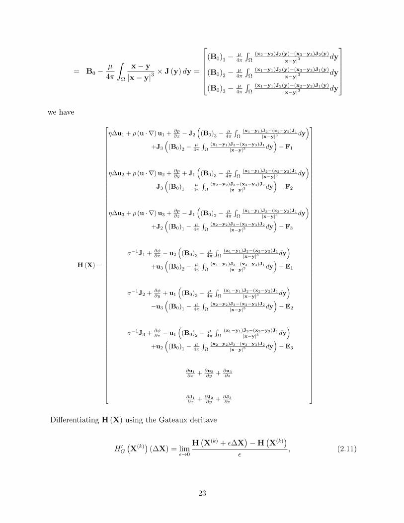
= B0 −µ

4π

∫Ω

x− y

|x− y|3× J (y) dy =

(B0)1 −

µ4π

∫Ω

(x2−y2)J3(y)−(x3−y3)J2(y)

|x−y|3 dy

(B0)2 −µ4π

∫Ω

(x1−y1)J3(y)−(x3−y3)J1(y)

|x−y|3 dy

(B0)3 −µ4π

∫Ω

(x1−y1)J2(y)−(x2−y2)J1(y)

|x−y|3 dy

we have

H (X) =

η∆u1 + ρ (u · ∇)u1 + ∂p∂x − J2

((B0)3 −

µ4π

∫Ω

(x1−y1)J2−(x2−y2)J1

|x−y|3 dy)

+J3

((B0)2 −

µ4π

∫Ω

(x1−y1)J3−(x3−y3)J1

|x−y|3 dy)− F1

η∆u2 + ρ (u · ∇)u2 + ∂p∂y + J1

((B0)3 −

µ4π

∫Ω

(x1−y1)J2−(x2−y2)J1

|x−y|3 dy)

−J3

((B0)1 −

µ4π

∫Ω

(x2−y2)J3−(x3−y3)J2

|x−y|3 dy)− F2

η∆u3 + ρ (u · ∇)u3 + ∂p∂z − J1

((B0)2 −

µ4π

∫Ω

(x1−y1)J3−(x3−y3)J1

|x−y|3 dy)

+J2

((B0)1 −

µ4π

∫Ω

(x2−y2)J3−(x3−y3)J2

|x−y|3 dy)− F3

σ−1J1 + ∂φ∂x − u2

((B0)3 −

µ4π

∫Ω

(x1−y1)J2−(x2−y2)J1

|x−y|3 dy)

+u3

((B0)2 −

µ4π

∫Ω

(x1−y1)J3−(x3−y3)J1

|x−y|3 dy)−E1

σ−1J2 + ∂φ∂y + u1

((B0)3 −

µ4π

∫Ω

(x1−y1)J2−(x2−y2)J1

|x−y|3 dy)

−u3

((B0)1 −

µ4π

∫Ω

(x2−y2)J3−(x3−y3)J2

|x−y|3 dy)−E2

σ−1J3 + ∂φ∂z − u1

((B0)2 −

µ4π

∫Ω

(x1−y1)J3−(x3−y3)J1

|x−y|3 dy)

+u2

((B0)1 −

µ4π

∫Ω

(x2−y2)J3−(x3−y3)J2

|x−y|3 dy)−E3

∂u1

∂x + ∂u2

∂y + ∂u3

∂z

∂J1

∂x + ∂J2

∂y + ∂J3

∂z

Differentiating H (X) using the Gateaux deritave

H ′G(X(k)

)(∆X) = lim

ε→0

H(X(k) + ε∆X

)−H

(X(k)

)ε

, (2.11)

23

where ∆X = X(k+1) − X(k) and ε∆X = ε (∆u1,∆u2,∆u3,∆p,∆J1,∆J2,∆J3) , we obtain

(see Appendix B) the Newton iteration

−η∇ · ∇u(k+1) + ρ(u(k+1) · ∇

)u(k) − ρ

(u(k) · ∇

)u(k) + ρ

(u(k) · ∇

)u(k+1)

+∇p(k+1) − J(k) × B(J(k+1)

)+ J(k) × B

(J(k)

)− J(k+1) ×B

(J(k)

)

σ−1J(k+1) +∇φ(k+1) − u(k) × B(J(k+1)

)+ u(k) × B

(J(k)

)− u(k+1) ×B

(J(k)

)

∇ · u(k+1)

∇ · J(k+1)

=

F

E

0

0

. (2.12)

Dropping off the first two terms from the linearization of each of the three nonlinear terms

of the equations, we have a Picard iteration [53]

−η∇ · ∇u(k+1) + ρ(u(k) · ∇

)u(k+1) +∇p(k+1) − J(k+1) ×B

(J(k)

)

σ−1J(k+1) +∇φ(k+1) − u(k+1) ×B(J(k)

)

∇ · u(k+1)

∇ · J(k+1)

=

F

E

0

0

.

We can see that these are the original equations with a component of each nonlinear term

being lagged to create the linearization. The corresponding weak formulation would then

be

η

∫Ω

(∇u(k+1)

): (∇v) + ρ+

∫Ω

((u(k) · ∇

)u(k+1)

)· v −

∫Ω

p(k+1) (∇ · v)−∫

Ω

(J(k+1) × B

(J(k)

))· v

−∫

Ω

(J(k+1) ×B0

)· v + σ−1

∫Ω

J(k+1) ·K +

∫Ω

∇φ(k+1) ·K−∫

Ω

(u(k+1) × B

(J(k)

))·K

−∫

Ω

(u(k+1) ×B0

)·K =

∫Ω

F · v +

∫Ω

E ·K∫Ω

(∇ · u(k+1)

)q +

∫Ω

J(k+1) · ∇ψ =

∫Γ

(Jext · n)ψ

24

Recalling the forms

a0 ((v1,K1) , (v2,K2)) := η

∫Ω

(∇v1) : (∇v2) + σ−1

∫Ω

K1 ·K2

+

∫Ω

((K2 ×B0) · v1 − (K1 ×B0) · v2) , (2.13)

a1 ((v1,K1) , (v2,K2) , (v3,K3)) :=ρ

2

∫Ω

(((v1 · ∇) v2) · v3 − ((v1 · ∇) v3) · v2)

+

∫Ω

((K3 × B (K1)) · v2 − (K2 × B (K1)) · v3) , (2.14)

and

b ((v,K) , (q, ψ)) := −∫

Ω

(∇ · v)P (q) +

∫Ω

K · (∇ψ) , (2.15)

we are now ready to state the convergent Picard iteration scheme proposed by Meir and

Schmidt for the numerical solution of Problem P h1 .

Iteration Scheme. Given(uh0 ,J

h0

)∈ Yh with uh0

∣∣Γ

= gh, for n ∈ N, find(uhn,J

hn

)∈ Yh

with uhn∣∣Γ

= gh and(phn, φ

hn

)∈Mh such that

a0

((uh(k+1),J

h(k+1)

),(vh,Kh

))+ a1

((uh(k),J

h(k)

),(uh(k+1),J

h(k+1)

),(vh,Kh

))+ b((

vh,Kh),(ph(k+1), φ

h(k+1)

))=

∫Ω

F · vh +

∫Ω

E ·Kh

and

b((

uh(k+1),Jh(k+1)

),(qh, ψh

))=

∫Γ

(Jext · n)ψh

for all(vh,Kh

)∈ Xh and

(qh, ψh

)∈Mh. For further details, we refer to [78].

25

Chapter 3

Matrix System and Preconditioner

3.1 Matrix Formulation

Restating the convergent Picard iteration scheme with n in place of k + 1,

a0

((uh(n),J

h(n)

),(vh,Kh

))+ a1

((uh(n−1),J

h(n−1)

),(uh(n),J

h(n)

),(vh,Kh

))+ b((

vh,Kh),(ph(n), φ

h(n)

))=

∫Ω

F · vh +

∫Ω

E ·Kh

and

b((

uh(n),Jh(n)

),(qh, ψh

))=

∫Γ

(Jext · n)ψh

for all(vh,Kh

)∈ Xh and

(qh, ψh

)∈ Mh. The scheme is expanded using the definition of

a0, a1, and b

η

∫Ω

∇uh(n) : ∇vh + σ−1

∫Ω

Jh(n) ·Kh +

∫Ω

(Kh ×B0

)· uh(n) −

∫Ω

(Jh(n) ×B0

)· vh

+ρ

∫Ω

((uh(n−1) · ∇

)uh(n)

)· vh +

∫Ω

(Kh × B

(Jh(n−1)

))· uh(n) −

∫Ω

(Jh(n) × B

(Jh(n−1)

))· vh

−∫

Ω

ph(n)∇ · vh +

∫Ω

∇φh(n) ·Kh =

∫Ω

F · vh +

∫Ω

E ·Kh

−∫

Ω

∇ · uh(n)q +

∫Ω

Jh(n)∇ψh =

∫Γ

(Jext · n)ψ

Choosing a basis for each of the finite-dimensional subspaces~φuk

nhuk=1⊂ Yh

1 ,~φJk

nhJk=1⊂ Yh

2 ,

φpknhpk=1 ⊂ Mh

1 , andφφk

nhφk=1⊂ Mh

2 , we can write the unknowns of problem P h1 as a linear

26

combination of the respective basis

ph(n) =

nhp∑k=1

c(p,n)k ϕ

(p)k

uh(n) =

nhu∑k=1

c(u,n)k ~ϕ

(u)k

φh(n) =

nhφ∑k=1

c(φ,n)k ϕ

(φ)k

Jh(n) =

nhJ∑k=1

c(J,n)k ~ϕ

(J)k

Substituting this representation into the iteration scheme and and using distributive prop-

erties of the gradient, divergence, cross product and dot product we have

nhu∑i=1

c(u,n)i η

∫Ω

∇~ϕ(u)i : ∇~ϕ(u)

j +

nhJ∑i=1

c(J,n)i σ−1

∫Ω

~ϕ(J)i · ~ϕ

(J)k

+

nhu∑i=1

c(u,n)i

∫Ω

(~ϕ

(J)k × ~B0

)· ~ϕ(u)

i −nhJ∑i=1

c(J,n)i

∫Ω

(~ϕ

(J)i × ~B0

)· ~ϕ(u)

j

+

nhu∑i=1

c(u,n)i ρ

∫Ω

((~uh(n−1) · ∇

)~ϕ

(u)i

)· ~ϕ(u)

j +

nhu∑i=1

c(u,n)i

∫Ω

(~ϕ

(J)k × ~B

(~Jh(n−1)

))· ~ϕ(u)

i

−nhJ∑i=1

c(J,n)i

∫Ω

(~ϕ

(J)i × ~B

(~Jh(n−1)

))· ~ϕ(u)

j −nhp∑i=1

c(p,n)i

∫Ω

ϕ(p)i ∇ · ~ϕ

(u)j

+

nhφ∑i=1

c(φ,n)i

∫Ω

∇ϕ(φ)i · ~ϕ

(J)k =

∫Ω

F · ~ϕ(u)j +

∫Ω

E · ~ϕ(J)k

and

−nhu∑i=1

c(u,n)i

∫Ω

∇ · ~ϕ(u)i ϕ

(p)l +

nhJ∑i=1

c(J,n)i

∫Ω

~ϕ(J)i · ∇ϕ(φ)

m =

∫Γ

( ~Jext · ~n)ϕ(φ)l .

27

Letting

A(u) =[a

(u)(i,j)

]:=

[η

∫Ω

∇~ϕ(u)i : ∇~ϕ(u)

j

]1 ≤ i ≤ nu, 1 ≤ j ≤ nu,

A(J) =[a

(J)(i,k)

]:=

[σ−1

∫Ω

~ϕ(J)i · ~ϕ

(J)k

]1 ≤ i ≤ nJ , 1 ≤ k ≤ nJ ,

B(p) =[b

(p)(i,l)

]:=

[∫Ω

ϕ(p)l ∇ · ~ϕ

(u)i

]1 ≤ i ≤ nu, 1 ≤ l ≤ np,

B(φ) =[b

(φ)(i,m)

]:=

[∫Ω

~ϕ(J)i · ∇ϕ(φ)

m

]1 ≤ i ≤ nJ , 1 ≤ m ≤ nφ,

C =[c(i,k)

]:=

[∫Ω

(~ϕ

(J)k × ~B0

)· ~ϕ(u)

i

]1 ≤ i ≤ nu, 1 ≤ k ≤ nJ ,

N(u) =[n

(u)(i,j)

]:=

[ρ

∫Ω

((~uh(n−1) · ∇

)~ϕ

(u)i

)· ~ϕ(u)

j

]1 ≤ i ≤ nu, 1 ≤ j ≤ nu,

and

N(J) =[n

(J)(i,k)

]:=

[∫Ω

(~ϕ

(J)k × ~B

(~Jh(n−1)

))· ~ϕ(u)

i

]1 ≤ i ≤ nu, 1 ≤ k ≤ nJ

denote the matrices formed by the respective terms of the iteration scheme, given on the

right-hand side of each definition. We group the coordinates from each linear combination of

the uknowns of problem P h1 into a vector. We do that same for the respective right-hand sides

of each equation of the iteration scheme, and for the sake of simplicity reuse the notations

F and E.

c(u,n) :=[c

(u,n)1 . . . c

(u,n)i . . . c(u,n)

nu

]t,

c(p,n) :=[c

(p,n)1 . . . c

(p,n)i . . . c(p,n)

np

]t,

c(J,n) :=[c

(J,n)1 . . . c

(J,n)i . . . c(J,n)

nJ

]t,

c(φ,n) :=[c

(φ,n)1 . . . c

(φ,n)i . . . c(φ,n)

nφ

]t,

F =

[∫Ω

F · φ(u)1 . . .

∫Ω

F · φ(u)j . . .

∫Ω

F · φ(u)nu

]t,

E =

[∫Ω

E · φ(J)1 . . .

∫Ω

E · φ(J)k . . .

∫Ω

E · φ(J)nJ

]t,

28

and

G =

[∫Γ

~Jextϕ(φ)1 . . .

∫Γ

~Jextϕ(φ)l . . .

∫Γ

~Jextϕ(φ)nφ

]t.

With these definitions we can write the iterative scheme in a matrix form

A(u) +N(u) Bt(p) −

(N(J) + C

)t0

B(p) 0 0 0

N(J) + C 0 A(J) Bt(φ)

0 0 B(φ) 0

c(u,n)

c(p,n)

c(J,n)

c(φ,n)

=

F

0

E

G

.

3.2 Finite Element Spaces

We choose finite element spaces for our finite-dimensional spaces. Recalling from [78] that

the spaces must satisfying the LBB-conditions

infqh∈Mh

1

supvh∈Yh

1

∫Ω

(∇ · vh

)qh

‖vh‖Yh1‖qh‖Mh

1

≥ β1 > 0

and

infψh∈Mh

2

supKh∈Yh

2

∫Ω

Kh ·(∇ψh

)‖Kh‖Yh

2‖ψh‖Mh

2

≥ β2 > 0,

we determine velocity-pressure pairs(Xh

1 ,Mh1

)and the current-potential pairs

(Xh

2 ,Mh2

).

The LBB condition for the velocity-pressure pair appears in the theory on the Stokes and

Navier-Stokes equations. Taylor-Hood elements are examples of velocity-pressure finite-

element pairs that satisfy the condition. For Taylor-Hood elements we choose triquadratics

for the velocity and trilinears for the pressure.

29

(a) Q1 Trilinear Nodes. (b) Q1 Basis Function.

Figure 3.1: 2-D Example of Q1 Basis Function for Pressure

(a) Q2 Triquadratic Nodes.(b) 2D Q2 Basis Function.

Figure 3.2: 2-D Example of Q2 Basis Function for Velocity

For each component k of the velocity vector basis function ~ϕ(u)i we use triquadratic elements

of the form

(ϕ

(φ)i (x)

)k

=∑

i1, i2, i3 ≥ 0

i1 + i2 + i3 ≤ 2

αi1,i2,i3xi11 x

i22 x

i33 ∈

Π1≤i≤3

(αi0 + αi1xi + αi2x

2i

): αij ∈ R

.

For the pressure basis functions ϕ(p)i , we use trilinears

ϕ(p)i (x) =

∑i1, i2, i3 ≥ 0

i1 + i2 + i3 ≤ 1

αi1,i2,i3xi11 x

i22 x

i33 ∈ Π1≤i≤3 (αi0 + αi1xi) : αij ∈ R .

To satisfy the LBB condition for the current density and electric potential pairs, we chose

triquadratic elements for the electric potential and Nedelec elements of the first kind and

30

second degree for the current density [81, 92, 17],

~ϕ(J)i (x)Pk =

u =

u1

u2

u3

: u1 ∈ Qk−1,k,k, u2 ∈ Qk,k−1,k, u3 ∈ Qk,k,k−1

.

where k = 2. For example, with k = 2 the first component u1 is located in the tensor product

of a linear in x, quadratic in y, and quadratic in z. u1 will be linear and discontinuous in x

and quadratic and continuous in y and z. These properties of the Nedelec element are due

to the degrees of freedom having the form [17]

∫e

u · τ qds ∀q ∈ Pk−1 (e) ,

1

|f |

∫f

(u× n) · qdA, ∀q ∈ (Pk−2 (f))3 ,

and ∫K

u · qdV, ∀q ∈ (Pk−3 (K))3 ,

where K is a reference element, e is an edge of K, f is a face of K, τ is the unit vector along

the edge e, and Pk is the linear space of polynomials of degree ≤ k. Note p ∈ Pk if and only

if

p(x) =∑

i1, i2, i3 ≥ 0

i1 + i2 + i3 ≤ k

αi1,i2,i2xi11 x

i22 x

i33

3.3 Preconditioner

We are now in a position to numerically solve the linear system. Having chosen GMRES to

solve the system, we consider the preconditioner. To solve the system efficiently, we wish to

minimize the number of iterations to convergence of the iterative solver. Hence we consider

31

bounds on the size of the residual rn = b − Axn, since the tolerance on this value indicates

when the solver has converged. In particular, we have the theorem [95]

Theorem 3.1 At step n of the GMRES iteration for the system Ax = b, the residual rn =

b− Axn satisfies

‖rn‖ = ‖pn(A)b‖ ≤ infpn∈Pn

‖pn(A)‖ ‖b‖ ≤ κ(V ) infpn∈Pn

‖pn‖Λ(A) ‖b‖

where Λ (A) is the set of eigenvalues of A, V is a nonsingular matrix of eigenvectors (as-

suming A is diagonalizable), Pn = p a polynomial : degree (p) ≤ n, p(0) = 1 and ‖pn‖Λ(A)

is defined by

‖pn‖Λ(A) = supz∈Λ(A)

pn (z) : z ∈ Λ (A) ⊂ R, pn ∈ Pn

From the theorem, we conclude that if the system matrix A is normal, then a small condition

number for the matrix of eigenvectors V will decrease the estimate on ‖rn‖ and help to reduce

the number of iterations to reach convergence. Perhaps more importantly, polynomials in

Pn existing such that their values when applied to A have a small norm will also decrease

the bound on the residual. More can be said if the matrix A is normal. The norm on the

polynomials is considered over the spectrum of A (Λ (A)). If n is small then the zeros of the

polynomial would also be small. For this to occur, the number of eigenvalues of A would

have to be small or grouped together in a small number of clusters m. With this in mind,

we consider our matrix system

A(u) +N(u) Bt(p) −

(N(J) + C

)t0

B(p) 0 0 0

N(J) + C 0 A(J) Bt(φ)

0 0 B(φ) 0

c(u,n)

c(p,n)

c(J,n)

c(φ,n)

=

F

0

E

G

.

32

To construct a preconditioner, we start by considering the work done for the Stokes and

Navier-Stokes equations. These equations correspond to the upper left 2-by-2 block of our

system matrix. Successful constructions of preconditioners for this system have been carried

out by Elman, Silvester and Wathen [37]. The lower-right two-by-two block of our system

is similar in form to the Navier-Stokes system. We therefore plan to extend the work of

Elman, Silvester and Wathen to this portion of our system. To the best of our knowledge,

this extension to our system can not be found in the literature. As a first preconditioner

we construct one that is block-diagonal, and based on the system after removal of the terms

due to the nonlinearities u×B (magnetic induction), J×B (the Lorentz force), and u · ∇u

(the interial term). We therefore plan to construct a preconditioner for the system

A(u) Bt(p) 0 0

B(p) 0 0 0

0 0 A(J) Bt(φ)

0 0 B(φ) 0

and

A Bt

B 0

=

A(u)... Bt

(p) 0

0 A(J)... 0 Bt

(φ)

. . . . . . . . . . . .

B(p) 0... 0 0

0 B(φ)... 0 0

.

For the Stokes equations, Elman, Silvester and Wathen developed a block-diagonal precon-

ditioner using the pressure Schur complement S(p) = BpA−1u Bt

p. Their preconditioner was

P1 =

A−1u 0

0 BpA−1u Bt

p

To extend their work, we consider the potential Schur complement S(φ) = B(φ)A

−1(J)B

t(φ)

and make plans to use it to precondition the lower-right 2-by-2 block of our system in a

similar manner. Following their work, we recall the definition of the pressure mass matrix

Q(p) =[q

(p)ij

]=[∫

Ωϕ

(p)i ϕ

(p)j

]along with the following theorem about its spectral equivalence

with the pressure Schur complement matrix S(p) [37].

33

Theorem 3.2 For any flow problem with a Dirichlet boundary condition and discretized

using a uniformly stable mixed approximation on a shape regular, quasi-uniform subdivision

of R3, the pressure Schur complement matrix B(p)A−1(u)B

t(p) is spectrally equivalent to the

pressure mass matrix Q(p):

β21 ≤

⟨B(p)A

−1(u)B

t(p)q,q

⟩⟨Q(p)q,q

⟩ ≤ 1 ∀q ∈ Rnp such that q 6= 1

and further

β21 ≤

⟨Bt

(p)Q−1(p)B(p)v,v

⟩⟨A(u)v,v

⟩ ≤ 1 for all v ∈ Rnu with v /∈ null(B(p)

).

A definition for spectral equivalence is given below [96].

Definition 1 Consider two sequences of Hermitian positive definite matrices Ah and Ch

and assume that all the eigenvalues λ of C−1h Ah satisfy c1 < λ < c2 with positive c1 and c2

independent of h. Then Ah and Ch are said to be spectrally equivalent.

From the definition, we can see that Ch is a good preconditioner for the system matrix Ah

in terms of GMRES, since the preconditioned system’s eigenvalues cluster between c1 and

c2. The definition holds for Q(p) and B(p)A−1(u)B

t(p) upon considering the eigenvalue problem

Q−1(p)B(p)A

−1(u)B

t(p)x = λx. and the resultant inner product

⟨B(p)A

−1(u)B

t(p)x,x

⟩= λ

⟨Q−1

(p)x,x⟩

.

The bounds from the theorem give the desired result. Hence, pressure mass matrix Q(p) is a

good preconditioner for pressure Schur complement B(p)A−1(u)B

t(p).

To construct, a preconditioner for the lower right 2-by-2 block, we define the laplace potential

mass matrix Q(∇φ) =[q

(∇φ)ij

]=[∫

Ω∇ϕ(φ)

i · ∇ϕ(φ)j

]and state and prove a corresponding

theorem.

34

Theorem 3.3 For any uniformly stable mixed approximation for the electric potential and

current-density on a shape regular, quasi-uniform subdivision of R3, the potential Schur

complement matrix S(φ) = B(φ)A−1(J)B

t(φ) is spectrally equivalent to the laplace potential mass

matrix Q(∇φ):

β22 ≤

⟨B(φ)A

−1(J)B

t(φ)q,q

⟩⟨Q(∇φ)q,q

⟩ ≤ 1 ∀q ∈ Rnφ such that q 6= 1.

The condition number of the potential Schur complement satisfies

κ(S(φ)

)=λmax (Sφ)

λmin (Sφ)<

C

β22c.

To make clear some of the statements in the theorem, we give definitions for shape regular

and quasi-uniform [37] and prove a lemma. Let Th be a decomposition of a convex polyhedral

domain of interest into hexahedral “brick” elements ∆k, and let h(k)x , h

(k)y , and h

(k)z be the

lengths of the brick element ∆k in the x, y, and z directions, respectively. We call a sequence

of hexahedral meshes Th shape regular [37] if there exists a maximum brick edge ratio

γ∗ such that every brick element ∆k ∈ Th satisfies 1 ≤ γ∆k≤ γ∗, where

γ∆k= max

(h

(k)x

h(k)y

,h

(k)x

h(k)z

,h

(k)y

h(k)x

,h

(k)y

h(k)z

,h

(k)z

h(k)x

,h

(k)z

h(k)y

).

From this definition, we see that the ratio of the longest edge to the shortest edge of each

element ∆k is bounded from above and below, and the uniform boundedness guarantees

that the elements do not degenerate with refinement. Letting hk denote the length of the

longest edge of ∆k, we call the sequence of meshes Th quasi-uniform [37] if there exists

a constant ρ > 0 such that

min∆k∈Th

hk ≥ ρ max∆k∈Th

hk

(with max

∆k∈Thhk ≥ min

∆k∈Thhk

).

35

for every mesh in the sequence. The definition implies that the local mesh size hk is about

constant for each mesh, with the ratio of the largest local mesh size to the smallest local

mesh size bounded between 1ρ

and 1, and these bounds carry over with each refinement.

Lemma 3 Using a Q2 triquadratic element approximation of the electric potential on a

shape-regular subdivision in R3 for which a shape regular condition holds, the laplace potential

mass matrix Q(∇φ) approximates the scaled identity matrix in the sense that

ch3 ≤⟨Q(∇φ)q,q

⟩〈q,q〉

≤ Ch3 ∀q ∈ Rnφ ,

where h = max∆k∈Th hk and the constants c and C are independent of h.

Proof:

First, note that Q(∇φ) =[∫

Ω∇ϕ(φ)

i · ∇ϕ(φ)j

]is symmetric and positive definite. In particular,

0 ≤∥∥∥∇φh∥∥∥2

L2(Ω)=

∫Ω∇φh · ∇φh =

∫Ω∇φh · ∇

nφ∑i=1

c(φ)i ϕ

(φ)i =

nφ∑i=1

c(φ)i

∫Ω∇φh · ∇ϕ(φ)

i

=

[∫Ω∇φ

h · ∇ϕ(φ)1 . . .

∫Ω∇φ

h · ∇ϕ(φ)nφ

]c

(φ)1

...

c(φ)nφ

=

[∑nφj=1 c

(φ)j

∫Ω∇ϕ

(φ)j · ∇ϕ

(φ)1 . . .

∑nφj=1 c

(φ)j

∫Ω∇ϕ

(φ)j · ∇ϕ

(φ)nφ

]c

(φ)1

...

c(φ)nφ

=

[c

(φ)1 . . . c

(φ)nφ

]∫

Ω∇ϕ(φ)1 · ∇ϕ(φ)

1 . . .∫

Ω∇ϕ(φ)1 · ∇ϕ(φ)

nφ

.... . .

...∫Ω∇ϕ

(φ)nφ · ∇ϕ

(φ)1 . . .

∫Ω∇ϕ

(φ)nφ · ∇ϕ

(φ)nφ

c

(φ)1

...

c(φ)nφ

=⟨Q(∇φ)c

(φ), c(φ)⟩.

36

We can therefore form a basis for Rnφ out of the eigenvectors of Q(∇φ) and denote the

minimum and maximum eigenvalues as λmin and λmax respectively, with

λmin 〈q,q〉 ≤⟨Q(∇φ)q,q

⟩≤ λmax 〈q,q〉 ∀q ∈ Rnφ .

Consider an arbitrary element ∆k of the grid Th. Letting Q(k)(∇φ) =

[∫∆k∇ϕ(φ)

i · ∇ϕ(φ)j

], we

have Q(∇φ) =∑

k∈Th Q(k)(∇φ) and

0 ≤∥∥φh∥∥2

L2(∆k)=⟨Q

(k)(∇φ)c

(φ), c(φ)⟩.

With Q(k)(∇φ) symmetric and positive definite, the same is true for 1

h(k)x h

(k)y h

(k)z

Q(k)(∇φ). Similar to

Q(∇φ), we have

λ(k)min 〈q,q〉 ≤

⟨1

h(k)x h

(k)y h

(k)z

Q(k)(∇φ)q,q

⟩≤ λ(k)

max 〈q,q〉 ∀q ∈ Rnφ .

Shape regularity of the triangulations Th implies that there exists a maximum brick edge

ratio γ∗ such that every element ∆k ∈ Th satisfies 1 ≤ γ∆k≤ γ∗. Without loss of generality,

let h(k)x ≤ h

(k)y ≤ h

(k)z = hk. Then h

(k)x

h(k)z

<h

(k)y

h(k)z

< 1 and γ∆k= h

(k)z

h(k)x

>h

(k)y

h(k)x

> 1. With

h(k)x h(k)

y h(k)z =

h(k)x

h(k)z

h(k)y

h(k)z

(h(k)z

)3=

1

γ∆k

h(k)y

h(k)z

h3k ≥

1

γ∆k

h(k)x

h(k)z

h3k ≥

1

γ2∆k

h3k ≥

1

γ∗h3k

and

h(k)x h(k)

y h(k)z =

h(k)y

h(k)x

h(k)z

h(k)x

(h(k)x

)3 ≤ h(k)y

h(k)x

h(k)z

h(k)x

h3k ≤

h(k)z

h(k)x

h(k)z

h(k)x

h3k = γ2

∆kh3k ≤ γ2

∗h3k,

we have

h3k

1

γ2∗λ

(k)min 〈q,q〉 ≤ h(k)

x h(k)y h(k)

z λ(k)min 〈q,q〉 ≤

⟨Q

(k)(∇φ)q,q

⟩≤ h(k)

x h(k)y h(k)

z λ(k)max 〈q,q〉 ≤ h3

kγ2∗λ

(k)max 〈q,q〉 .

37

The sequence of triangulations Th are quasi-uniform and there exists a constant ρ > 0

such that min∆k∈Th hk ≥ ρmax∆k∈Th hk. With h = max∆k∈Th hk we have

ρ3h3 1

γ2∗λ

(k)min 〈q,q〉 ≤

⟨Q

(k)(∇φ)q,q

⟩≤ h3γ2

∗λ(k)max 〈q,q〉

and since⟨Q(∇φ)q,q

⟩=∑

∆k∈Th

⟨Q(k)q,q

⟩we have

ρ3h3 1

γ2∗〈q,q〉

n∆k∑k=1

λ(k)min ≤

⟨Q(∇φ)q,q

⟩≤ h3γ2

∗ 〈q,q〉n∆k∑k=1

λ(k)max.

Letting c = ρ3

γ2∗

∑n∆

k=1 λ(k)min and C = γ2

∗∑n∆k

k=1 λ(k)max, gives

ch3 ≤⟨Q(∇φ)q,q

⟩〈q,q〉

≤ Ch3 q ∈ Rnφ .

We now prove Theorem 3.3.

Proof:

The lower bound of the inequality that we wish to establish is a consequence of the LBB

condition

β2 ≤ minψh 6=constant

max~Kh 6=~0

∣∣(Kh,∇ψh)∣∣

‖ψh‖1,Ω ‖Kh‖0,Ω

.

We start first with the upper bound. Writing the components from the numerator of the

LBB condition as linear combinations of basis functions

Kh =

nJ∑i=1

ki~ϕ(J)i = ϕt(J)k and ψh =

nφ∑i=1

qiϕ(φ)i = ϕt(φ)q,

38

the integral in the numerator of the LBB condition can then be written as

∫Ω

Kh · ∇ψh =

nJ∑i=1

ki

nφ∑j=1

qj

∫Ω

~ϕ(J)i · ∇ψhj =

⟨k, Bt

(φ)q⟩.

For the denominator we have

∥∥∥ ~Kh∥∥∥2

L2(Ω)=

∫Ω

~Kh · ~Kh =

nJ∑i=1

ki

nJ∑j=1

kj

∫Ω

~ϕ(J)i · ~ϕ

(J)j =

⟨A(J)k,k

⟩and

∥∥ψh∥∥2

L2(Ω)=

∫Ω

ψhψh +∇ψh · ∇ψh

=

nφ∑i=1

qi

nφ∑j=1

qj

∫Ω

ϕ(φ)i ϕ

(φ)j +

nφ∑i=1

qi

nφ∑j=1

qj

∫Ω

∇ϕ(φ)i · ∇ϕ

(φ)j

=⟨q, Q(φ)q

⟩+⟨q, Q(∇φ)q

⟩=⟨q,(Q(φ) +Q(∇φ)

)q⟩≤⟨q, Q(∇φ)q

⟩,

since Q(φ) and Q(∇φ) are symmetric positive definite. With A(J) symmetric positive definite

we can diagonalize it with a matrix P and define its root

A(J) = PDP−1 and A1/2(J) = PD1/2P−1.

Thus,

∣∣⟨k, Bt(φ)q

⟩∣∣ =∣∣∣( ~Kh,∇ψh

)∣∣∣ ≤ ∥∥Kh∥∥

(L2(Ω))3

∥∥∇ψh∥∥L2(Ω)

=√⟨

k, A(J)k⟩√〈q, Q∇φq〉

and we obtain the upper bound

∣∣∣⟨k, Bt(φ)q

⟩∣∣∣√⟨k, A(J)k

⟩√〈q, Q∇+φq〉

≤ 1 ∀k ∈ RnJ ∀q ∈ Rnφ .

39

In particular, for k = A−1(J)B

t(φ)q we have

√⟨B(φ)A

−1(J)B

t(φ)q,q

⟩√⟨

q, Q(∇φ)q⟩ ≤ 1 ∀q ∈ Rnφ .

For the lower bound, we start with the LBB condition

β2 ≤ minψh 6=const

max~Kh 6=~0

∣∣∣∫Ω~Kh · (∇ψh)

∣∣∣∥∥∥ ~Kh∥∥∥

(L2(Ω))3‖ψh‖H1(Ω)

= minq 6=1

maxk 6=0

∣∣∣⟨k, Bt(φ)q

⟩∣∣∣√⟨k, A(J)k

⟩√⟨q,(Q(φ) +Q(∇φ)

)q⟩

≤ minq 6=1

maxk 6=0

∣∣∣⟨k, Bt(φ)q

⟩∣∣∣√⟨k, A(J)k

⟩√⟨q, Q(∇φ)q

⟩ = minq 6=1

1√⟨q, Q(∇φ)q

⟩ maxk 6=0

∣∣∣⟨k, Bt(φ)q

⟩∣∣∣√⟨k, A(J)k

⟩= min

q 6=1

1√⟨q, Q(∇φ)q

⟩ maxw 6=0

∣∣∣⟨A−1/2(J) w, Bt

(φ)q⟩∣∣∣√⟨

A1/2(J)k, A

1/2(J)k

⟩ = minq 6=1

1√⟨q, Q(∇φ)q

⟩ maxw 6=0

∣∣∣⟨w, A−1/2(J) Bt

(φ)q⟩∣∣∣√

〈w,w〉

= minq 6=1

1√⟨q, Q(∇φ)q

⟩⟨A−1/2(J) Bt

(φ)q, A−1/2(J) Bt

(φ)q⟩

√⟨A−1/2(J) Bt

(φ)q, A−1/2(J) Bt

(φ)q⟩ = min

q 6=1

√⟨B(φ)A

−1(J)B

t(φ)q,q

⟩√⟨

q, Q(∇φ)q⟩ .

The maximum is attained when w = ±A−1/2(J) Bt

(φ)q. This can be seen by incorporating the

norm of w in the denominator into the first term of inner product in the numerator and

recalling the scalar product formula |a| |b| cos (θ) = 〈a,b〉. The largest absolute value will

occur when the unit vector w√〈w,w〉

is in the same direction or opposite direction of the other

vector. The two inequalities yield the result

β22 ≤

⟨B(φ)A

−1(J)B

t(φ)q,q

⟩⟨Q(∇φ)q,q

⟩ ≤ 1 ∀q ∈ Rnφ such that q 6= 1

Using the previous lemma, we have the bounds

β22ch

3 < λmin

(B(φ)A

−1(J)B

t(φ)

)〈q,q〉 ≤

⟨B(φ)A

−1(J)B

t(φ)q,q

⟩≤ λmax

(B(φ)A

−1(J)B

t(φ)

)< Ch3 ∀q ∈ Rnφ with q 6= 1

40

and the condition number of the potential Schur complement satisfies

κ(B(φ)A

−1(J)B

t(φ)

)=λmax

(B(φ)A

−1(J)B

t(φ)

)λmin

(B(φ)A

−1(J)B

t(φ)

) <C

β22c

Corollary 1 From the eigenvalues σ of

A−1(J) 0

0 Q−1

0 Bt

(φ)

B(φ) 0

k

ψ

= σ

k

ψ

we have that

β22 ≤

⟨Bt

(φ)Q−1(∇φ)B(φ)k,k

⟩⟨A(J)k,k

⟩ ≤ 1 ∀k ∈ RnJ such that k /∈ null(B(φ)

)

Proof: We consider two cases σ = 0 and σ 6= 0. For the case σ = 0 with

[kt ψt

]t6= 0

(eigenvalue problem), the preconditioning matrix on the left is nonsingular and therefore

implies that Bt(φ)ψ = 0 and B(φ)k = 0. Conversely, if k 6= 0 and ψ 6= 0 with Bt

(φ)ψ = 0 and

B(φ)k = 0, then σ = 0. Looking at the individual rows we have

Bt(φ)ψ = σA(J)k and B(φ)k = σQψ.

Therefore ⟨k, Bt

(φ)ψ⟩

= σ⟨A(J)k,k

⟩and

⟨ψ, B(φ)k

⟩= σ 〈Qψ,ψ〉 .

Further,⟨A(J)k,k

⟩= 〈Qψ,ψ〉, if σ 6= 0. From this equality and the positive definiteness of

A(J) and Q(∇ψ), σ 6= 0 implies k 6= 0 and ψ 6= 0. Our interest is thus in the case σ 6= 0.

41

Multiplying the system by the diagonal matrix shown below

B(φ) 0

0 Bt(φ)

A−1

(J) 0

0 Q−1

0 Bt

(φ)

B(φ) 0

k

ψ

= σ

B(φ) 0

0 Bt(φ)

k

ψ

we can write each row in terms of a single component of the eigenvector

B(φ)A−1(J)B

t(φ)ψ = σB(φ)k = σ2Qψ and Bt

(φ)Q−1(φ)B(φ)k = σBt

(φ)ψ = σ2A(J)k.

Hence, we obtain two related eigenvalue problems

Q−1B(φ)A−1(J)B

t(φ)ψ = σ2ψ and A−1

(J)Bt(φ)Q

−1(φ)B(φ)k = σ2k.

Further, ⟨B(φ)A

−1(J)B

t(φ)ψ,ψ

⟩〈Qψ,ψ〉

= σ2 =

⟨Bt


⟩⟨A(J)k,k

⟩ .

The positive definiteness of Q(∇φ) and that of the potential Schur complement from the

previous theorem, we have nφ positive eigenvalues σ2. By this relation and the previous

theorem, we obtain

β22 ≤

⟨Bt


⟩⟨A(J)k,k

⟩ ≤ 1

as desired.

Following similar arguments as in [37] we formulate the block-diagonal preconditioner that

we will use for our problem. In the following theorem we look at its effects on the eigenvalues

of the simplified system.

Theorem 3.4 If uh, ph and Jh,φh have uniformly stable mixed approximations such that

spectral equivalence of the Schur complements with the mass matrices hold, then for the

42

system

A−1(u) 0 0 0

0 A−1(J) 0 0

0 0 Q−1(p) 0

0 0 0 Q−1(∇φ)

A(u) 0 Bt(p) 0

0 A(J) 0 Bt(φ)

B(p) 0 0 0

0 B(φ) 0 0

u

J

p

φ

= λ

u

J

p

φ

all negative eigenvalues satisfy

−1 ≤ λ ≤ 1

2−√

1 + 4 min (β1, β2)

2,

and all positive eigenvalues satisfy

1 ≤ λ ≤ 1

2+

√5

2.

Upon replacing Q(p) and Q(∇φ) by the corresponding Schur complements, the system has

exactly three eigenvalues λ = 1, 12±√

52

.

Proof:

Let x =

u

J

and y =

p

φ

. Define A,B, and Q by

A Bt

B 0

x

y

: =

A(u) 0 Bt(p) 0

0 A(J) 0 Bt(φ)

B(p) 0 0 0

0 B(φ) 0 0

u

J

p

φ

43

= λ

A(u) 0 0 0

0 A(J) 0 0

0 0 Q(p) 0

0 0 0 Q(∇φ)

u

J

p

φ

=: λ

A 0

0 Q

x

y

.

Proving the last part of the theorem first, replace Q by the block diagonal matrix BA−1Bt

of the pressure and potential Schur complements . The result follows from consideration of

two cases: y = 0 and y 6= 0.

For y = 0 we have x 6= 0 else our eigenvector is the zero vector. Looking at the second row

of the system: Ax +Bty = λAx, we see Ax = λAx. Using the positive definiteness of A, we

have 〈Ax,x〉 > 0 and therefore λ = 1.

For y 6= 0, we set the first and second row of the system equal to each other. From the

second row of the system, we have Bx = λQy = λBA−1Bty and therefore

(λ− 1)Bx = (λ− 1)λBA−1Bty.

Solving the first row Ax +Bty = λAx for Bty and multiplying by BA−1 we have

Bty = (λ− 1)Ax =⇒ BA−1Bty = (λ− 1)Bx.

Therefore, BA−1Bty = (λ− 1)λBA−1Bty and with BA−1Bt positive definite (from the last

theorem) we have 〈BA−1Bty,y〉 > 0 and

1 = (λ− 1)λ with λ =1

2±√

5

2.

using the quadratic formula.

44

To determine the intervals from the first part of the theorem, we consider the two cases λ < 0

and λ > 0. Suppose that λ < 0 is an eigenvalue of the system. We claim this implies that

y 6= 0. In contradiction, suppose that y = 0. Then x 6= 0 to have a meaningful eigenvalue

problem. Looking at the first row of the system, we have Ax + Bty = λAx. Since y = 0,

Ax = λAx. With A positive definite, and x 6= 0 it must be that λ = 1 > 0, a contradiction.

The first row of the system Ax + Bty = λAx also implies that x = 1λ−1

A−1Bty. We can

substitute this result for x into the second row of the system Bx = λQy, and obtain

1

λ− 1BA−1Bty = λQy and BA−1Bty = λ (λ− 1)Qy = −λ (1− λ)Qy.

The positive definiteness and spectral equivalence of the Schur complements with their cor-

responding mass matrices along with λ < 0 imply

−λ 〈Qy,y〉 ≤ −λ (1− λ) 〈Qy,y〉 =⟨BA−1By,y

⟩≤ 〈Qy,y〉 .

With y 6= 0 we have λ ≥ −1. From the lower bounds of the spectral equivalences

−λ (1− λ) 〈Qy,y〉 =⟨BA−1Bty,y

⟩≥ min (β1, β2) 〈Qy,y〉 .

Hence, λ2 − λ−min (β1, β2) ≥ 0. Factorizing, we have (λ− λ+) (λ− λ−) ≥ 0, where

λ± =1

2±√

1 + 4 min (β1, β2)

2.

From λ ≥ λ+ or λ ≤ λ−, and we obtain the upper bound λ ≤ 12−√

1+4 min(β1,β2)

2. With the

bounds −1 ≤ λ ≤ 12−√

1+4 min(β1,β2)

2established for λ < 0, we are ready to look at the last

case λ > 0.

For λ > 0 we have that x 6= 0. Suppose by contradiction that x = 0. Then, having an

eigenvalue problem with λ > 0 it must be that y 6= 0. Taking an inner product of the second

45

row of the system Bx = 0 = λQy with y implies that y = 0, since Q(∇φ) positive definite

and λ > 0.

Equating the first and second row of the system by way of the inner product 〈Bty,x〉 =

〈Bx,y〉, we have

(λ− 1) 〈Ax,x〉 = λ 〈Qy,y〉 ≥ 0.

And with x 6= 0, we have λ ≥ 1. For the upper bound, the second row provides y = 1λQ−1Bx,

and we substitute this into the first row

(λ− 1)Ax = Bty =1

λBtQ−1Bx.

From the previous corollary, we have

(λ− 1) 〈Ax,x〉 =1

λ

⟨1

λBtQ−1Bx,x

⟩≤ 1

λ〈Ax,x〉

and x 6= 0 implies that λ2 − λ− 1 ≤ 0. Completing the square, we have(λ− 1

2

)2 −√

52

2≤ 0

and the difference of squares gives the upper bound λ ≤ 12

+√

52

.

The theorem on the block-diagonal preconditioner can be made more general as in [37].

Rather than using A in the preconditioner, spectral equivalence of A with a simpler matrix

is used in establishing eigenvalue bounds, However, the theorem above will allow us to make

comparisons in the next chapter. In particular, we will see the effect of the preconditioner

from the theorem on eigenvalues of the simplified system for a particular example.

46

Chapter 4

Computational Experiments and Results

4.1 Introduction to the Computational Environment

4.1.1 Choice of the Libraries

The deal.ii library was used to implement the finite element method, p4est was used to

partition the domain to the nodes of the distributed memory cluster, and a GMRES im-

plementation from Trilinos was used to approximate the solution of the linear system in

parallel as well invoke part of the preconditioner. Freely available libraries were also used for

mesh generation and solution visualization. The open source library Gmsh [43] was used to

generate several meshes, and the open-source library VisIt [22, 23, 100] was used to visualize

the approximated solution.

Successful meshes were generated using Gmsh with particular coding techniques applied to

the Gmsh script file and alterations to output .msh files (removing all but volume elements).

The techniques were necessary, since Gmsh generates meshes using triangles in two dimen-

sions and tetrahedrons in three dimensions (n-simplices), where deal.ii works with meshes

that are quadrilaterals in two dimensions and and hexahedrals in three dimensions. There-

fore, using Gmsh required unconventional coding in its script language in order to obtain

hexahedral three-dimensional meshes.

The need for care with Gmsh was first noticed with Navier-Stokes benchmark tests for flow

around a cylinder discussed by Turek and Schaefer [87]. During these tests it became evident

47

(a) Velocity Field with Presure Contours

(b) Velocity Vector Field

Figure 4.1: Schafer Turek Benchmark

that boundary conditions were not being properly enforced for the velocity. Nonzero veloc-

ities were occurring on the boundary where zero velocities were prescribed. After trouble-

shooting the code, it became clear that the grid was causing problems. Some web research

48

concerning Gmsh and hexahedrals lead to editing of the Gmsh script files and the output

.msh files. The problem with the boundary was fixed by removing elements in the out-

put .msh file that were not volume elements (see GMSH manual http://geuz.org/gmsh/).

Results comparable to Schafer and Turek were obtained as seen in the figure 4.1. With in-

creasing library of meshes offered by newer versions of deal.ii and continued obstacles using

Gmsh for generation, Gmsh was replaced by the deal.ii library for mesh generation toward

the end of this research. In particular, code was added to the deal.ii library to create a

toroidal mesh. A factor that appears to have influenced this decision was the activity of the

mailing list. The depth of resources and documentation became important with increased

investment in a library.

All of the visualization of data conducted during this research was performed using the library

VisIt. VisIt was initially developed and is supported by the Lawrence Livermore National

Lab. VisIt has decent documentation. However, the lack of documentation on movies with

resolution providing crisp clarity have brought into consideration review of other libraries

such as Paraview for comparison of capabilities and documentation.

4.1.2 Working with the Libraries

It should be mentioned that problems running code with the libraries can, do and have

occurred during development. It is difficult to recall all bugs and problems encountered.

They range from a variety of sources. Problems may occur in the installation process of the

open-source libraries. This can be due to compiling a library with a faulty or unsupported

compiler, attempting to link different libraries that have not been compiled with the same

compiler, trying to link to versions of libraries that a particular library does not support,

trying to link shared and static libraries, or not being able to properly locate and link to

a compiler that has been installed by a system administrator. Bugs may also occur in the

code being developed, such as a segmentation fault for an incorrectly set vector size. Bugs

49

may be found in the codes of the libraries that are being used, such as a bug encountered

with the deal.ii PETSc vector values associated with ghost cells not being properly zeroed or

a bug encountered with deal.ii function calls that work properly for serial code but corrupt

for parallel code - as in mesh generation problems for an L-shaped domain. Bugs may

occur that allow the code to compile and run but give unexpected results. An example

is the approximate solution to the continuous pressure solutions of example 1 that gave

discontinuous pressure contours. Rather than set the pressure at a node, the mean value

pressure was calculated and then subtracted off the solution. This change in determining

the unique solution eliminated the discontinuity appearing in the pressure contours. As the

code was developed this problem eventually disappeared when both methods were retested.

Attempts to recreate the bug have been unsuccessful. Most problems can be traced to a

source, however some may disappear for uknown reasons with code development.

Bugs can occur outside of code run time, such as during visualization or mesh creation. An

example of this type of problem is mentioned with the opensource software Gmsh opensource

software when creating the flow around a cylinder to test out the Navier Stokes code while

developing toward the MHD code. The problem appeared to be creating hexahedral elements

using software designed to create tetrahedral elements. The problem was successfully over-

come for a mesh used to model the flow around a cylinder in a rectangular duct. However,

the problem was encountered again with the torus mesh with no apparent fix. Fortunately,

deal.ii’s mesh generation capabilities were developed enough to add code to the library to

create a torus from hexhedral elements.

The use of multiple libraries can be forboding. The cause of an error may appear (and can

be) difficult to determine or understand. In troubleshooting all the bugs encountered, the

location of the bug was found first. Then, to understand the bug’s behavior, adjustments to

the code were made. Examples are changing the sample problem being tested or the size of

a vector. The most common bugs occurred at interfaces between libraries. Important tips

50

to minimize work in tracking bugs are developing, programming, compiling and testing code

frequently and in increments.

4.2 Example 1 - A Problem with an Exact Solution

The parallel finite element code was tested for expected convergence rates on two different

domains: the cube [0, 1]3 and an L-shaped domain

[0, 1]3⋃

x+ (0, 1, 0) : x ∈ [0, 1]3⋃

x+ (1, 1, 0) : x ∈ [0, 1]3,

Using the example problem from [78]

u (x, y, z) :=

0

−π cos(πx) exp(−s)(

12− z)

−π cos(πx) exp(−s)(y − 1

2

)

J (x, y, z) :=

2 sin(πx)(1− s) exp(−s)


2

)−π cos(πx) exp(−s)

(z − 1

2

)

p (x, y, z) := −1

2sin2 (πx) s exp(−2s),

φ (x, y, z) :=2

πcos(πx),

B (x, y, z) :=

1

sin(πx) exp(−s)(

12− z)

sin(πx) exp(−s)(y − 1

2

)

with r =(0, y − 1

2, z − 1

2

)and s = |r|2 =

(y − 1

2

)2+(z − 1

2

)2. Note that u and B are

divergence free and ∇×B = J (see Appendix D). The above set of equations is therefore a

smooth solution to the velocity-current magnetohydrodynmaic equations with all parameters

51

η, ρ,σ, and µ equal to unity and the data F, E, g, Jext, and Bext defined by

F := −∆u + (u · ∇)u +∇p− J×B,= −

∇ · ∇u1

∇ · ∇u2

∇ · ∇u3

+

u · ∇u1

u · ∇u2

u · ∇u3

+

px

py

pz

−J2B3 − J3B2

J3B1 − J1B3

J1B2 − J2B1

=

0

π cos(πx) exp(−s)(z − 1

2

) (π2 + 9− 4s

)+ sin2(πx) exp(−2s)

(y − 1

2

)−π2 cos2(πx) exp(−2s)

(y − 1

2


(y − 1

2

) (π2 + 9− 4s


(z − 1

2


(z − 1

2

)

E := J +∇φ− u×B =

2 sin(πx) ((1− s) exp(−s)− 1)

0

0

and

g := u∣∣Γ, Jext := J

∣∣R3\Ω, Bext := i.

Further, instead of integrating the Biot-Savart formula over R3\Ω, the magnetic field induced

by Jext can be obtained from B −Bext − B(J∣∣Ω

). For uniqueness of the pressure and the

electric potential, the exact solutions above for the pressure and potential were adjusted by

a constant

p (x, y, z) := −1

2sin2 (πx) s exp(−2s)− p,

φ (x, y, z) :=2

πcos(πx)− 2

π,

52

where p = 1Ω

∫Ω−1

2sin2 (πx) s exp(−2s)dx was the mean pressure value of the exact solution

over the domain Ω. For the electric potential φ one of the degrees of freedom on the x = 0

boundary of the domain [0, 1]3 was set to the value of the electric potential φ at x = 0 (

φ(0) = 0 ) by using the deal.ii constraint matrix.

The rates of convergence on the cube and the L-shaped domain are given in the tables 4.1

and 4.2.

Table 4.1: Errors and Convergence Rates for the Unit Cube Domain

Domain Infomation u J p φ# Cells # DOFs Cell size (h) H1-error L2-error L2-error H1-error

H1-rate L2-rate L2-rate H1-rate

512 34,253 0.125 0.015004 0.000573 0.008111 0.006400(8x8x8)

4096 253,205 0.0625 0.003751 0.000136 0.002031 0.001602(16x16x16) 2.000000 2.019216 1.999429 1.999674

32,768 1,945,637 0.03125 0.000938 0.000034 0.000508 0.000401(32x32x32) 1.999615 2.000000 1.999290 1.998200

Table 4.2: Errors and Convergence Rates for the Lshaped Domain



24 2183 0.5 0.404921 0.146763 0.0154336 0.217988(2x2x2)

192 13,969 0.25 0.102145 0.037215 0.00490111 0.00558378(4x4x4) 2.000000 2.076676 1.997737 1.998621

1536 44,508 0.125 0.02557343 0.00933088 0.000997906 0.0140478(8x8x8) 2.000001 2.019216 1.999429 1.999674

Visualizations of the numerical approximations to the solution of this example (see Figure

4.2) show symmetry about the line at the intersection of the planes x = 12

and y = 12. Note

that to obtain illustrative perspectives in the plots for each variable, the point of view for

each variable’s plot is slightly different as indicated by the axes in the lower left corner. In

particular, to compare the velocity vector field with the pressure contour plot, the pressure

53

(a) Current in Cube Domain - Example 1 (b) Potential in Cube Domain - Example 1

(c) Velocity in Cube Domain - Example 1 (d) Pressure in Cube Domain - Example 1

Figure 4.2: Example 1 for Cube Domain

plot would have to be rotated 90 degrees counter-clockwise around the z-axis. The symmetry

in each plot would then match.

Approximate solutions to the problem on an L-shaped domain were also obtained. with

graphs of the results shown in figure 4.3. From the figure, we see that the L-shaped domain

extends the profiles of each approximated function occurring on the cube domain.

4.3 Example 2 - An Applied Problem

Approximate solutions to a second problem with more realistic conditions were also obtained

for the unit cube and L-shaped domains. The problem prescribed a current entering at one

54

(a) Current in L-shaped Domain - Ex 1 (b) Potential in L-shaped Domain - Ex 1

(c) Velocity in L-shaped Domain - Ex 1 (d) Pressure in L-shaped Domain - Ex 1

Figure 4.3: Example 1 for Lshaped Domain

55

end (part of a domain face parallel to the z-axis) of the domain and exiting at the an end

opposite to the entrance. The Dirichlet boundary conditions for the velocity were zero and

the external magnetic field was zero for the problem as well. The magnitude of the current

entering and exiting the domain through the boundary was fixed at |Jext| = 100. In order

to obtain a unique solution for the electric potential and pressure, the problem was handled

similar to the previous problem with an exact solution. In particular, the pressure mean

value was calculated in a post process and subtracted from the solved pressure solution. The

results can be seen in Figures 4.4, 4.5 and 5.2.

(a) Current in Cube Domain - Example 2 (b) Potential in Cube Domain - Example 2

(c) Velocity in Cube Domain - Example 2 (d) Pressure in Cube Domain - Example 2

Figure 4.4: Example 2 for Cube Domain

The current density vector field plots exhibit the current entering and exiting the domain, as

indicated above. This can be seen for both the cube and L-shaped domains, where the current

56

(a) Current in L-shaped Domain - Ex 2 (b) Potential in L-shaped Domain - Ex 2

(c) Velocity in L-shaped Domain - Ex 2 (d) Pressure in L-shaped Domain - Ex 2


travels into and out of the domain in the same direction. Since the external magnetic field is

zero, the induced magnetic field described by the Biot-Savart formula is the only contributor

to the forces experienced by the fluid - the Lorentz force J×B in the momentum equation.

In the vector field plot for the velocity, we can see that maximum fluid speeds are occurring

in the center of the domain with an upward direction. Again, the only driving force for this

flow is the Lorentz force J × B due to the induced magnetic field. In consideration of the

Biot-Savart formula and the symmetry of the current-density in the domain, we see that

the upward maximum velocity occurring in the center may be expected. The BiotSavart

formula provides for large contributions to the induced magnetic field in regions where the

57

magnitudes J (y) of the current are large as well as where the distances |x− y| are small. We

see that the current magnitudes are largest at the boundary. In calculating the Biot-Savart

integrand at the center of the domain x = (1/2, 1/2, 1/2) and incorporating the negative

sign from outside the integral, vectors pointing in the direction of the negative x-axis for

both exiting and entering currents on the boundary are obtained. Likewise, close to the

center of the domain y where the distance |x− y| to the center x is small, the negative

cross-product of the integrand again gives a direction toward the negative x-axis. With the

induced magnetic field at the center having this direction, we can determine the body force

acting on the fluid at this location by taking the cross product of this field with the current

moving in the direction of the positive y-axis. This cross product yields an upward-pointing

Lorentz force in the positive z-direction. This upward body force acting on the fluid does

indeed correspond to the upward velocity profile seen at the center of the domain. Further,

the contributions noted on both sides of the plane y = 1/2 can only occur near the center

of the cube and imply a maximum magnitude there. The lack of domain symmetry with

respect to the entering and exiting current density of the L-shaped domain makes it harder

to argue the velocity profiles seen for this case.

4.3.1 Preconditioning Results

Returning to the second problem with the more realistic conditions and the cube domain, we

compare the expected theoretical results to computed computational results for the eigen-

values of this problem. Recall the form of our preconditioner

P =

A−1(u) 0 0 0

0 Q−1(p) 0 0

0 0 A−1(J) 0

0 0 0 Q−1(∇φ)

,

58

where Q(p) is the pressure mass matrix and Q(∇φ) is the laplacian mass matrix.

For each eigenvalue plot, we have considered the second iteration in the Picard iteration

sequence. We plot the eigenvalues on the complex plane for the unit cube refined once

in each direction to yield 8 cells. We start with the plot of the eigenvalues of the system

matrix before preconditioning, shown in 4.6. From this plot, we can see that the eigenvalues

are not clustered in groups, especially near the origin. We may expect that the number of

GMRES iterations to convergence to be high, and indeed without a preconditioner GMRES

fails converge (for the default tolerance and maximum number of iterations).

Figure 4.6: Eigenvalues for System Matrix

Next, we examine the eigenvalue plot in figure 4.7 for simplified system of theorem 3.4 after

applying our preconditioner. From the plot, we can see clustering in three locations. Looking

closely, we see the locations are exactly the eigenvalues stated in the last part of the theorem

when constructing the preconditioner by using the Schur complements instead of the mass

59

matrices. It appears that constructing with the mass matrices gives the same result. Roughly

twenty eigenvalues are located away from the three clusters. These eigenvalues are believed

to be due to the velocity boundary conditions enforced by deal.ii by way of the system matrix

[12, 1]. Further, a zero eigenvalue can be seen in the graph. This was determined to be due

to the null space of the pressure having dimension one. We note that GMRES did not have

a problem with convergence for such a system.

Figure 4.7: Eigenvalues for Preconditioned Stokes-Ohms System

Finally, we look at the effects of preconditioning on the eigenvalues for the simplified system

with the inertial term, figure 4.8, and for the simplified system with both the inertial term

and Lorentz force terms (the entire system matrix), figure 4.9. From these plots, we see

that clustering of eigenvalues is still occurring, though not as well as for only the simplified

system. We note that GMRES still converged with less than 100 iterations.

60

Figure 4.8: Eigenvalues for Preconditioned Stokes-Ohms System with Inertial Term

Figure 4.9: Eigenvalues for Preconditioned System Matrix

61

Chapter 5

Conclusion and Future Work

5.1 Summary

We have implemented a parallel, object-oriented, finite element code that utilizes open-

source, academic and government software libraries. The code is capable of approximating

the solution to the velocity-current MHD equations on high performance computer clusters.

We have established a preconditioner that permits using GMRES to approximate the solution

to the system of equations iteratively. We have successfully tested the code on the unit cube

and an L-shaped domain for two problem types. For the problem with an exact solution we

have obtained expected orders of convergence [78]. We have also successfully run the code

with millions of unknowns on a 64 node distributed memory architecture at the Alabama

Supercomputer Center DMC. From these results and opportunities to discuss our work, we

have a couple different directions that we would like to develop in the future that will be

outlined in the upcoming sections.

5.2 Torus Domain

Discussions with physicists have indicated a potential for the velocity-current equations

to model plasma in fusion reactors. Two general types of fusion reactors are stellarators

(named after the devices purpose of harnessing the power of a stellar object - the sun) and

tokomaks (a Russion acronym, due to its origin). The main difference between a tokomak

and a stellarator are their methods of generating the magnetic fields that confine the plasma.

The stellarator uses two magnetic fields generated by currents running through coils that

62

surround the plasma. The tokomak generates one field by running current through a set

of coils encircling the plasma, but creates the second field by sending current through the

plasma. Our system of equations appears to apply naturally to the tokamak reactor design,

with a current being applied to the domain to create the second magnetic field. We note that

research on fusion energy is active, with fusion energy being an engineering grand challenge

problem for the 21st century and grants being available through the NSF on fusion energy

research. In fact, the ITER (International Thermonuclear Experimental Reactor) project

located in the south of France is the largest tokomak reactor in the world and has been

designed to be the first full scale fusion power plant. We can see that With the domain

of a tokomak being essentially a torus, we have interest in approximating solutions to our

equations for a toroidal domain. We have started testing out equations on this domain. In

particular, we are testing the first problem from chapter 3, having an exact solution, on a

quarter torus. Results at this time are located in in the figure 5.1 and table 5.1.

Table 5.1: Errors and Convergence Rates for the Quarter Torus Domain



80 5553 h1 0.132016 0.0270524 0.0257992 0.0828241

640 40,261 12h1 0.0349727 0.00647049 0.0134858 0.0214727

1.916412 2.063810 0.935884 1.947547

5120 306,597 14h1 0.00894921 0.00164881 0.0129277 0.00552349

1.966397 1.972450 0.060975 1.958852

From the convergence table for the quarter-torus we see the expected rates of approximation,

except for the pressure. Work continues on this problem to understand the problematic rate

of convergence for the pressure. We have seen a similar situation with the L-shaped domain

and will be testing our code with this in mind.

63

(a) Current in Torus Domain - Ex 1 (b) Potential in Torus Domain - Ex 1

(c) Velocity in Torus Domain - Ex 1 (d) Pressure in Torus Domain - Ex 1


(a) Current in Torus Domain - Ex 2 (b) Potential in Torus Domain - Ex 2

64

(c) Velocity in Torus Domain - Ex 2 (d) Pressure in Torus Domain - Ex 2

Figure 5.2: Example 2 for Torus Domain

We have also obtained results on the quarter-torus domain for the second example of chapter

3. In this case the current can be seen entering and exiting through the cross-sections of

the torus (see Figure 5.2), with the directions of entry and departure perpendicular to each

other. The predictions for the velocity and the pressure are interesting. According to the

velocity vector field, the fluid does not appear to be cycling through to torus in the xy-plane,

but rather the movement is vertical and along the torus’s radial cross-sections. At the angle

of capture of the velocity graph, this may be difficult to see. The layers of the pressure

contours also correspond to the movement of the fluid into and out of the torus’ radial axis,

with high pressures located along that axis.

Finally, we have started numerical approximations of the equations on a full torus. Related

to the second example of chapter three with the velocity at the boundary being zero and

the current entering and exiting a particular part of the domain, we have the results seen in

figure 5.3

65

(a) Current in Full Torus Domain - Ex 2 (b) Potential in Full Torus Domain - Ex 2

(c) Velocity in Full Torus Domain - Ex 2 (d) Pressure in Full Torus Domain - Ex 2

Figure 5.3: Example 2 for Full Torus Domain

5.3 Code Speedup

Another research direction is the consideration of code bottlenecks. We have started work in

this direction by comparing the three slowest components of the code: the assembly of the

equation system, the solution of the system and the calculation of the Biot-Savart integral at

each quadrature point during the assembly. In the plots in figure 5.4, we quickly see that the

slowest component of the code during runtime is the calculation of the Biot-Savart integral.

Figure 5.4 considers strong scaling, where the problem size (the number of unknowns or

domain refinement) has been fixed and the number of processors is varied. We recall that

the speedup for a parallel program under a fixed problem size is the ratio of the parallel

66

program’s time over the sequential program’s time. Ideally, if two processors are used instead

of one, then the time to complete a portion of code should decrease by a factor of two, and

the speedup would be 2. In our observations, as we double the number of processors we

use to numerically approximation the solution to the equations of fixed mesh size, we see

(in the plot on the left in figure 5.4) that the time to completion is roughly halved for each

of the components of the code being considered. Recall that parallel efficiency is the ratio

of speedup over the number of processors, and that ideal efficiency has a value of 1. We

conclude from the graphs that the libraries being used in the assembly (deal.ii) and the

solution (trilinos) of the system of equations have good parallel efficiency in this range of

processors for this particular problem size. From the graphs as well, the in-house MPI code

for the BiotSavart integral also exhibits the same level of efficiency in this processor range.

To see the speedup and efficiency more clearly, we use a log-log plot with a base of two.

Doubling the number of processors corresponds to incrementing by one unit on the x-axis,

and halving the cpu time corresponds to a decrease on the y-axis by one unit. We expect

in the ideal case that an increment of one unit along the x-axis would result in a decrease

of one unit along the y-axis, and that we would see a linear trend in the log-log plot with a

slope of negative one. The plot on the right in figure 5.4 does indeed show trends close to

ideal.

With the three slowest components working near optimal efficiency with respect to strong

scaling observations, we would like to address the slowest component of the code, the Biot-

Savart integral. The Biot-Savart integral calculates the magnetic field induced by the current

density in the domain. The code does this using quadrature. Each processor contains

information - previous current densities and quadrature points - needed to perform the

quadrature calculation over the domain for a particular location x in

B (Jn−1) (x) = − µ

4π

∫Ω

x− y|x− y|3

× Jn−1 (y) dy

67

Figure 5.4: CPU Time Versus Number of Processors

to determine the value of the Biot-Savart integral at that particular location. With all

the information readily available on each processor (after a numerical solve), the major

component of the calculation is the MPI communication between processors. To see if

we can shorten the time to approximate the induced magnetic field at these locations, we

consider approximating the solution to the magnetic field in the Maxwell equations

∇ ·B = 0 and ∇×B = J(n−1) on Ω

with the boundary condition

68

B · n = B (Jn−1) · n

by a parallel finite element method, using deal.ii. We approximate the solution to the system

of equations using the least squares finite element method [67, 19]. Just as with the solution

method using only the Biot-Savart integral, the obtained magnetic field values are used in

the next solve for the four uknowns J, u, p, φ. For the first example problem from chapter

three with exact solutions, we look at strong scaling using this method, and compare this

to the Biot-Savart method. Note that the method using only the Biot-Savart integral was

optimized to make the comparison as fair as possible - leading to considerable reductions

that can be seen when comparing figure 5.5 to 5.4. However, even with optimizations to the

communication occurring during the Biot-Savart method, we can see that the solution of the

div-curl system is almost an order of magnitude faster and appears to parallelize well.

As can be seen in the figure 5.5, we even tested an approximation to the BiotSavart integral

method, where we used the fact that the denominator in the integrand of the BiotSavart

integral caused the magnetic field values to be small with large distances between x and y.

This method was a first step toward a fast multipole method for the integral [24, 47, 13, 46,

93, 64]. However, the least squares finite element method to calculate the induced magnetic

field in the domain outperformed this simplifying approximation to the quadrature method

for the BiotSavart integral. This div-curl finite element solver for the induced magnetic field

seems to be a natural direction for future work. For future work, we would like to do some

analysis on this code and extend this code to domains that are nonconvex. A major issue

is the possible occurrence of singularities in such a domains [26]. Hence, the geometry of

the domain must be taken into consideration [27, 14, 63, 28] with the possible use of the

discontinuous finite element method. It may also be of interest to address the problem from

the point of view of finite element exterior calculus [61, 6, 4, 5].

69

Figure 5.5: CPU Time Versus Number of Processors

70

Appendices

71

Appendix A

Weak Formulation and Identities

A.1 Navier-Stokes Identities

Here, we go over the identities

∫Ω

v · ∇p = −∫

Ω

p∇ · v +

∫∂Ω

pn · v

−∫

Ω

v · ∇2u =

∫Ω

∇u : ∇v −∫∂Ω

(n · ∇u) · v

ρ

∫Ω

((u · ∇) u) · v =ρ

2

(∫Ω

((u · ∇) u) · v −∫

Ω

((u · ∇) v) · u)

to write Navier-Stokes equations in the form below.

∫Ω

F · v = −η∫

Ω

∆u · v + ρ

∫Ω

((u · ∇) u) · v +

∫Ω

∇p · v

= η

∫Ω

∇u : ∇v +ρ

2

(∫Ω

((u · ∇) u) · v −∫

Ω

((u · ∇) v) · u)−∫

Ω

p∇ · v

A.1.1 Pressure Term

We weaken the pressure in the term∫

Ω∇p · v by using

∂

∂x(v · a) =

∂

∂x(v1a1 + v2a2 + v3a3)

= v1∂a1

∂x+∂v1

∂xa1 + v2

∂a2

∂x+∂v2

∂xa2 + v3

∂a3

∂x+∂v3

∂xa3

72

= v ·(∂

∂xa

)+

(∂

∂xv

)· a

to form the identity

∇ · (pv) =

⟨∂pv1

∂x,∂pv2

∂y,∂pv3

∂z

⟩=

⟨p∂v1

∂x+ v1

∂p

∂x, p∂v2

∂y+ v2

∂p

∂y, p∂v3

∂z+ v3

∂p

∂z

⟩= v · ∇p+ p∇ · v.

Using this result with the divergence theorem∫

Ω∇ · v =

∫∂Ω

v · n we have

∫Ω

v · ∇p = −∫

Ω

p∇ · v +

∫Ω

∇ · (pv)

= −∫

Ω

p∇ · v +

∫∂Ω

pn · v

A.1.2 Diffusion Term

The diffusion term∫

Ω∇2u · v is weakened using integration by parts and the identity

∇ · (∇~u · ~v) = ∇~u : ∇~v + ~v · ∇2~u

Writing the gradient of the velocity vector in matrix form

∇u =

∂∂x

∂∂y

∂∂z

[u1 u2 u3

]=

∂u1

∂x∂u2

∂x∂u3

∂x

∂u1

∂y∂u2

∂y∂u3

∂y

∂u1

∂z∂u2

∂z∂u3

∂z

(A.1)

73

The diffusion term can then be written as

∆u = ∇2u = ∇ · (∇u) =

[∂∂x1

∂∂x2

∂∂x3

]u1,x u2,x u3,x

u1,y u2,y u3,y

u1,z u2,z u3,z

=

∂2u1

∂x2 + ∂2u1

∂y2 + ∂2u1

∂z2

∂2u2

∂x2 + ∂2u2

∂y2 + ∂2u2

∂z2

∂2u3

∂x2 + ∂2u3

∂y2 + ∂2u3

∂z2

=

∇ · ∇u1

∇ · ∇u2

∇ · ∇u3

=⟨∇2u1,∇2u2,∇2u3

⟩

Here we will write the tensor-tensor product ∇u : ∇v as

∇u : ∇v =

∂u1

∂x∂u2

∂x∂u3

∂x

∂u1

∂y∂u2

∂y∂u3

∂y

∂u1

∂z∂u2

∂z∂u3

∂z

:

∂v1

∂x∂v2

∂x∂v3

∂x

∂v1

∂y∂v2

∂y∂v3

∂y

∂v1

∂z∂v2

∂z∂v3

∂z

= u1,xv1,x + u1,yv1,y + u1,zv1,z + u1,xv2,x + u2,yv2,y + u2,zv2,z

+ u3,xv3,x + u3,yv3,y + u3,zv3,z

= (∇u1 · ∇v1) + (∇u2 · ∇v2) + (∇u3 · ∇v3)

(A.2)

Consider the divergence of the tensor-vector product ∇u · v

∇ · (∇u · v) = ∇ ·

∂u1

∂x∂u2

∂x∂u3

∂x

∂u1

∂y∂u2

∂y∂u3

∂y

∂u1

∂z∂u2

∂z∂u3

∂z

· v = ∇ ·

⟨(∂

∂xu

)· v,(∂

∂yu

)· v,(∂

∂zu

)· v⟩

=∂

∂x

(∂

∂xu · v

)+

∂

∂y

(∂

∂yu · v

)+

∂

∂z

(∂

∂zu · v

)=

(∂2u

∂x2· v +

∂v

∂x· ∂u

∂x

)+

(∂2u

∂y2· v +

∂v

∂y· ∂u

∂y

)(∂2u

∂z2· v +

∂v

∂z· ∂u

∂z

)= v · 〈∇ · ∇u1,∇ · ∇u2,∇ · ∇u3〉+ (∇v1 · ∇u1 +∇v2 · ∇u2 +∇v3 · ∇u3)

= v ·⟨∇2u1,∇2u2,∇2u3

⟩+∇v : ∇u = v · ∇2u +∇v : ∇u

74

Hence,

∫Ω

∇ · (∇u · v) =

∫Ω

v · (∇ · ∇u) +

∫Ω

∇u : ∇v

With the help of the divergence thereom, we can rewrite the diffusion term −∫

Ω∇2u · v in

Navier Stokes

−∫

Ω

v · ∇2u =

∫Ω

∇u : ∇v −∫

Ω

∇ · (∇u · v)

=

∫Ω

∇u : ∇v −∫∂Ω

(∇u · v) · n

=

∫Ω

∇u : ∇v −∫∂Ω

(n · ∇u) · v.

The last equality is true since

(∇u · v) · n =

∂u1

∂x∂u2

∂x∂u3

∂x

∂u1

∂y∂u2

∂y∂u3

∂y

∂u1

∂z∂u2

∂z∂u3

∂z

· v · n =

v · ∂

∂xu

v · ∂∂y

u

v · ∂∂z

u

· n= n1v ·

∂

∂xu + n2v ·

∂

∂yu + n3v ·

∂

∂zu =

(n1

∂

∂xu + n2

∂

∂yu + n3

∂

∂zu

)· v

=

(n ·⟨∂

∂xu,

∂

∂yu,

∂

∂zu

⟩)· v =

n ·

∂u1

∂x∂u2

∂x∂u3

∂x

∂u1

∂y∂u2

∂y∂u3

∂y

∂u1

∂z∂u2

∂z∂u3

∂z

· v

= (n · ∇u) · v

A.1.3 Advection Term

For the advection term, we wish to show

ρ

∫Ω

((u · ∇) u) · v =ρ

2

(∫Ω

((u · ∇) u) · v −∫

Ω

((u · ∇) v) · u)

75

To start,

ρ

∫Ω

((u · ∇) u) · v =ρ

2

∫Ω

((u · ∇) u) · v +ρ

2

∫Ω

((u · ∇) u) · v

=ρ

2

(∫Ω

((u · ∇) u) · v +

∫Ω

((u · ∇) u) · v)

We wish to show that

−∫

Ω

((u · ∇) u) · v =

∫Ω

((u · ∇) v) · u

we have that

((u · ∇) u) · v =

u1

∂u1

∂x+ u2

∂u1

∂y+ u3

∂u1

∂z

u1∂u2

∂x+ u2

∂u2

∂y+ u3

∂u2

∂z

u1∂u3

∂x+ u2

∂u3

∂y+ u3

∂u3

∂z

· v= v1

(u1∂u1

∂x+ u2

∂u1

∂y+ u3

∂u1

∂z

)+ v2

(u1∂u2

∂x+ u2

∂u2

∂y+ u3

∂u2

∂z

)+ v3

(u1∂u3

∂x+ +u2

∂u3

∂y+ u3

∂u3

∂z

)(A.3)

and that

((u · ∇) v) · u =

u1

∂v1

∂x+ u2

∂v1

∂y+ u3

∂v1

∂z

u1∂v2

∂x+ u2

∂v2

∂y+ u3

∂v2

∂z

u1∂v3

∂x+ u2

∂v3

∂y+ u3

∂v3

∂z

· u= u1

(u1∂v1

∂x+ u2

∂v1

∂y+ u3

∂v1

∂z

)+ u2

(u1∂v2

∂x+ u2

∂v2

∂y+ u3

∂v2

∂z

)+ v3

(u1∂v3

∂x+ +u2

∂v3

∂y+ u3

∂v3

∂z

)(A.4)

Using Integration-By-Parts and assuming that u∣∣Γ

= 0, we have

∫Ω

u1∂u1

∂x1

v1 =

∫Ω

(u1v1)∂u1

∂x1

= −∫

Ω

∂ (v1u1)

∂x1

u1 +

∫Γ

v1u1u1dS

76

= −∫

Ω

∂ (v1u1)

∂x1

u1 = −∫

Ω

v1∂ (u1)

∂x1

u1 −∫

Ω

u1∂ (v1)

∂x1

u1

Therefore,

∫Ω

v1

(u1∂u1

∂x+ u2

∂u1

∂y+ u3

∂u1

∂z

)+

∫Ω

v2

(u1∂u2

∂x+ u2

∂u2

∂y+ u3

∂u2

∂z

)+

∫Ω

v3

(u1∂u3

∂x+ +u2

∂u3

∂y+ u3

∂u3

∂z

)= −

∫Ω

v1∂u1

∂xu1 −

∫Ω

u1∂v1

∂xu1 −

∫Ω

v1∂u2

∂yu1 −

∫Ω

u2∂v1

∂yu1 −

∫Ω

v1∂u3

∂zu1 −

∫Ω

u3∂v1

∂zu1

−∫

Ω

v2∂u1

∂xu2 −

∫Ω

u1∂v2

∂xu2 −

∫Ω

v2∂u2

∂yu2 −

∫Ω

u2∂v2

∂yu2 −

∫Ω

v2∂u3

∂zu2 −

∫Ω

u3∂v2

∂zu2

−∫

Ω

v3∂u1

∂xu3 −

∫Ω

u1∂v3

∂xu3 −

∫Ω

v3∂u2

∂yu3 −

∫Ω

u2∂v3

∂yu3 −

∫Ω

v3∂u3

∂zu3 −

∫Ω

u3∂v3

∂zu3

(A.5)

Therefore, collecting terms we have

∫Ωv1

(u1∂u1

∂x+ u2

∂u1

∂y+ u3

∂u1

∂z

)+

∫Ωv2

(u1∂u2

∂x+ u2

∂u2

∂y+ u3

∂u2

∂z

)+

∫Ωv3

(u1∂u3

∂x+ +u2

∂u3

∂y+ u3

∂u3

∂z

)= −

(∫Ωu1∂v1

∂xu1 +

∫Ωu2∂v1

∂yu1 +

∫Ωu3∂v1

∂zu1

)−(∫

Ωv1∂u1

∂xu1 +

∫Ωv1∂u2

∂yu1 +

∫Ωv1∂u3

∂zu1

)−(∫

Ωu1∂v2

∂xu2 +

∫Ωu2∂v2

∂yu2 +

∫Ωu3∂v2

∂zu2

)−(∫

Ωv2∂u1

∂xu2 +

∫Ωv2∂u2

∂yu2 +

∫Ωv2∂u3

∂zu2

)−(∫

Ωu1∂v3

∂xu3 +

∫Ωu2∂v3

∂yu3 +

∫Ωu3∂v3

∂zu3

)−(∫

Ωv3∂u1

∂xu3 +

∫Ωv3∂u2

∂yu3 +

∫Ωv3∂u3

∂zu3

)(A.6)

Writing this in vector notation, we have

77

∫Ω

((u · ∇) u) · v =

∫Ω

(u · ∇u1) v1 + (u · ∇u2) v2 + (u · ∇u3) v3

= −∫

Ω

(u · ∇v1)u1 −∫

Ω

v1 (∇ · u)u1 −∫

Ω

(u · ∇v2)u2 −∫

Ω

v2 (∇ · u)u2

−∫

Ω

(u · ∇v3)u3 −∫

Ω

v3 (∇ · u)u3

= −∫

Ω

(u · ∇v1)u1 −∫

Ω

(u · ∇v2)u2 −∫

Ω

(u · ∇v3)u3 = −∫

Ω

((u · ∇) v) · u (A.7)

Hence,

ρ

∫Ω

((u · ∇) u) · v =ρ

2

(∫Ω

((u · ∇) u) · v +

∫Ω

((u · ∇) u) · v)

=ρ

2

(∫Ω

((u · ∇) u) · v −∫

Ω

((u · ∇) v) · u)

A.2 Ohms Law

We wish to show

∫Ω

(u×B) ·K = −∫

Ω

(K×B) · u.

This amounts to show that for any vector a, b, and c

∫Ω

(a× b) · c = −∫

Ω

(c× b) · a (A.8)

To start, recall that the cross product between two vectors a and b is

78

a× b = 〈a1, a2, a3〉 × 〈b1, b2, b3〉 =

∣∣∣∣∣∣∣∣∣∣i j k

a1 a2 a3

b1 b2 b3

∣∣∣∣∣∣∣∣∣∣=

∣∣∣∣∣∣∣a2 a3

b2 b3

∣∣∣∣∣∣∣ i−∣∣∣∣∣∣∣a1 a3

b1 b3

∣∣∣∣∣∣∣ j +

∣∣∣∣∣∣∣a1 a2

b1 b2

∣∣∣∣∣∣∣k= (a2b3 − a3b2) i− (a1b3 − a3b1) j + (a1b2 − a2b1) k (A.9)

Now, we wish to show that the identity

∫Ω

(a× b) · c = −∫

Ω

(c× b) · a (A.10)

is true.

First, note that a · (b× c) = (a× b) · c

a · (b× c) = 〈a1, a2, a3〉 · (〈b1, b2, b3〉 × 〈c1, c2, c3〉)

= 〈a1, a2, a3〉 · ((b2c3 − b3c2) i− (b1c3 − b3c1) j + (b1c2 − b2c1) k)

= a1 (b2c3 − b3c2)− a2 (b1c3 − b3c1) + a3 (b1c2 − b2c1)

= a1b2c3 − a1b3c2 − a2b1c3 + a2b3c1 + a3b1c2 − a3b2c1

= (a2b3 − a3b2) c1 − (a1b3 − a3b1) c2 + (a1b2 − a2b1) c3 = (a× b) · c (A.11)

Since a× b = −b× a and a · b = b · a

(a× b) · c = a · (b× c) = (b× c) · a = − (c× b) · a (A.12)

Therefore,

79

∫Ω

(a× b) · c = −∫

Ω

(c× b) · a (A.13)

80

Appendix B

Newton’s Method Linearization

Recalling Newton’s method

X(k+1) = X(k) −H(X(k)

)H′ (X(k))

(B.1)

with

H (X) =

η∆u1 + ρ (u · ∇)u1 + ∂p∂x − (J2B3 − J3B2)− F1

η∆u2 + ρ (u · ∇)u2 + ∂p∂y + (J1B3 − J3B1)− F2

η∆u3 + ρ (u · ∇)u3 + ∂p∂z − (J1B2 − J2B1)− F3

σ−1J1 + ∂φ∂x − (u2B3 − u3B2)−E1

σ−1J2 + ∂φ∂y − (u1B3 − u3B1)−E2

σ−1J3 + ∂φ∂z − (u1B2 − u2B1)−E3

∂u1

∂x + ∂u2

∂y + ∂u3

∂z

∂J1

∂x + ∂J2

∂y + ∂J3

∂z

and the variable X = (u1,u2,u3, p,J1,J2,J3, φ) obtained from the equations

−η∆u + ρ (u · ∇) u +∇p− J×B = F

σ−1J +∇φ− u×B = E,

∇ · u = 0 and ∇ · J = 0.

Also recall the Gateaux deritave

H ′G(X(k)

)(∆X) = lim

ε→0

H(X(k) + ε∆X

)−H

(X(k)

)ε

, (B.2)

81

where ∆X = X(k+1)−X(k) and ε∆X = ε (∆u1,∆u2,∆u3,∆p,∆J1,∆J2,∆J3) . Note that ∆

will be used for increment as opposed to using it for the Laplacian.

Since

B = B0 + B (J)

= B0 −µ

4π

∫Ω

x− y

|x− y|3× J (y) dy =

(B0)1 −

µ4π

∫Ω

(x2−y2)J3(y)−(x3−y3)J2(y)

|x−y|3 dy

(B0)2 −µ4π

∫Ω

(x1−y1)J3(y)−(x3−y3)J1(y)

|x−y|3 dy

(B0)3 −µ4π

∫Ω

(x1−y1)J2(y)−(x2−y2)J1(y)

|x−y|3 dy

82

we have

H(X(k)

)=

η∇ · ∇u(k)1 + ρ

(u(k) · ∇

)u

(k)1 + ∂p(k)

∂x

−J(k)2

((B0)3 −

µ4π

∫Ω

(x1−y1)J(k)2 −(x2−y2)J

(k)1

|x−y|3 dy

)+J

(k)3

((B0)2 −

µ4π

∫Ω

(x1−y1)J(k)3 −(x3−y3)J

(k)1

|x−y|3 dy

)− F1

η∇ · ∇u(k)2 + ρ

(u(k) · ∇

)u

(k)2 + ∂p(k)

∂y

+J(k)1

((B0)3 −

µ4π

∫Ω

(x1−y1)J(k)2 −(x2−y2)J

(k)1

|x−y|3 dy

)−J(k)

3

((B0)1 −

µ4π

∫Ω

(x2−y2)J(k)3 −(x3−y3)J

(k)2

|x−y|3 dy

)− F2

η∇ · ∇u(k)3 + ρ

(u(k) · ∇

)u

(k)3 + ∂p(k)

∂z

−J(k)1

((B0)2 −

µ4π

∫Ω

(x1−y1)J(k)3 −(x3−y3)J

(k)1

|x−y|3 dy

)+J

(k)2

((B0)1 −

µ4π

∫Ω

(x2−y2)J(k)3 −(x3−y3)J

(k)2

|x−y|3 dy

)− F3

σ−1J(k)1 + ∂φ(k)

∂x − u(k)2

((B0)3 −

µ4π

∫Ω

(x1−y1)J(k)2 −(x2−y2)J

(k)1

|x−y|3 dy

)+u

(k)3

((B0)2 −

µ4π

∫Ω

(x1−y1)J(k)3 −(x3−y3)J

(k)1

|x−y|3 dy

)−E1

σ−1J(k)2 + ∂φ(k)

∂y − u(k)1

((B0)3 −

µ4π

∫Ω

(x1−y1)J(k)2 −(x2−y2)J

(k)1

|x−y|3 dy

)+u

(k)3

((B0)1 −

µ4π

∫Ω

(x2−y2)J(k)3 −(x3−y3)J

(k)2

|x−y|3 dy

)−E2

σ−1J(k)3 + ∂φ(k)

∂z − u(k)1

((B0)2 −

µ4π

∫Ω

(x1−y1)J(k)3 −(x3−y3)J

(k)1

|x−y|3 dy

)+u

(k)2

((B0)1 −

µ4π

∫Ω

(x2−y2)J(k)3 −(x3−y3)J

(k)2

|x−y|3 dy

)−E3

∂u(k)1

∂x +∂u

(k)2

∂y +∂u

(k)3

∂z

∂J(k)1

∂x +∂J

(k)2

∂y +∂J

(k)3

∂z

and

83

H(X(k) + ε∆X

)=

η∇ · ∇(u

(k)1 + ε∆u1

)+ ρ

((u(k) + ε∆u

)· ∇) (

u(k)1 + ε∆u1

)+∂(p(k)+ε∆p)

∂x −(J

(k)2 + ε∆J2

)((B0)3 −

µ4π

∫Ω

(x1−y1)(J(k)2 +ε∆J2

)−(x2−y2)

(J(k)1 +ε∆J1

)|x−y|3 dy

)+(J

(k)3 + ε∆J3

)((B0)2 −

µ4π

∫Ω

(x1−y1)(J(k)3 +ε∆J3

)−(x3−y3)

(J(k)1 +ε∆J1

)|x−y|3 dy

)− F1

η∇ · ∇(u

(k)2 + ε∆u2

)+ ρ

((u(k) + ε∆u

)· ∇) (

u(k)2 + ε∆u2

)+

∂(p(k)+ε∆p)∂y

+(J

(k)1 + ε∆J1

)((B0)3 −

µ4π

∫Ω

(x1−y1)(J(k)2 +ε∆J2

)−(x2−y2)

(J(k)1 +ε∆J1

)|x−y|3 dy

)−(J

(k)3 + ε∆J3

)((B0)1 −

µ4π

∫Ω

(x2−y2)(J(k)3 +ε∆J3

)−(x3−y3)

(J(k)2 +ε∆J2

)|x−y|3 dy

)− F2

η∇ · ∇(u

(k)3 + ε∆u3

)+ ρ

((u(k) + ε∆u

)· ∇) (

u(k)3 + ε∆u3

)+

∂(p(k)+ε∆p)∂z

−(J

(k)1 + ε∆J1

)((B0)2 −

µ4π

∫Ω

(x1−y1)(J(k)3 +ε∆J3

)−(x3−y3)

(J(k)1 +ε∆J1

)|x−y|3 dy

)+(J

(k)2 + ε∆J2

)((B0)1 −

µ4π

∫Ω

(x2−y2)(J(k)3 +ε∆J3

)−(x3−y3)

(J(k)2 +ε∆J2

)|x−y|3 dy

)− F3

σ−1(J

(k)1 + ε∆J1

)+

∂(φ(k)+ε∆φ)∂x

−(u

(k)2 + ε∆u2

)((B0)3 −

µ4π

∫Ω

(x1−y1)(J(k)2 +ε∆J2

)−(x2−y2)

(J(k)1 +ε∆J1

)|x−y|3 dy

)+(u

(k)3 + ε∆u3

)((B0)2 −

µ4π

∫Ω

(x1−y1)(J(k)3 +ε∆J3

)−(x3−y3)

(J(k)1 +ε∆J1

)|x−y|3 dy

)−E1

σ−1(J

(k)2 + ε∆J2

)+

∂(φ(k)+ε∆φ)∂y

−(u

(k)1 + ε∆u1

)((B0)3 −

µ4π

∫Ω

(x1−y1)(J(k)2 +ε∆J2

)−(x2−y2)

(J(k)1 +ε∆J1

)|x−y|3 dy

)+(u

(k)3 + ε∆u3

)((B0)1 −

µ4π

∫Ω

(x2−y2)(J(k)3 +ε∆J3

)−(x3−y3)

(J(k)2 +ε∆J2

)|x−y|3 dy

)−E2

σ−1(J

(k)3 + ε∆J3

)+

∂(φ(k)+ε∆φ)∂z

−(u

(k)1 + ε∆u1

)((B0)2 −

µ4π

∫Ω

(x1−y1)(J(k)3 +ε∆J3

)−(x3−y3)

(J(k)1 +ε∆J1

)|x−y|3 dy

)+(u

(k)2 + ε∆u2

)((B0)1 −

µ4π

∫Ω

(x2−y2)(J(k)3 +ε∆J3

)−(x3−y3)

(J(k)2 +ε∆J2

)|x−y|3 dy

)−E3

∂(u

(k)1 +ε∆u1

)∂x +

∂(u

(k)2 +ε∆u2

)∂y +

∂(u

(k)3 +ε∆u3

)∂z

∂(J(k)1 +ε∆J1

)∂x +

∂(J(k)2 +ε∆J2

)∂y +

∂(J(k)3 +ε∆J3

)∂z

84

Then, since

ρ((

u(k) + ε∆u)· ∇)(

u(k)1 + ε∆u1

)= ρ

((u(k) + ε∆u

)· ∇)u

(k)1 + ρ

((u(k) + ε∆u

)· ∇)ε∆u1

= ρ(u(k) · ∇

)u

(k)1 + ρ (ε∆u · ∇)u

(k)1 + ρ

(u(k) · ∇

)ε∆u1

+ρ (ε∆u · ∇) ε∆u1

(J

(k)2 + ε∆J2

)(B0)3 −µ

4π

∫Ω

(x1 − y1)(J

(k)2 + ε∆J2

)− (x2 − y2)

(J

(k)1 + ε∆J1

)|x− y|3

dy

= J

(k)2

(B0)3 −µ

4π

∫Ω

(x1 − y1)(J

(k)2 + ε∆J2

)− (x2 − y2)

(J

(k)1 + ε∆J1

)|x− y|3

dy

+ε∆J2

(B0)3 −µ

4π

∫Ω

(x1 − y1)(J

(k)2 + ε∆J2

)− (x2 − y2)

(J

(k)1 + ε∆J1

)|x− y|3

dy

= J

(k)2

((B0)3 −

µ

4π

∫Ω

(x1 − y1)J(k)2 − (x2 − y2)J

(k)1

|x− y|3dy

)

+εJ(k)2

(0− µ

4π

∫Ω

(x1 − y1) ∆J2 − (x2 − y2) ∆J1

|x− y|3dy

)

+ε∆J2

((B0)3 −

µ

4π

∫Ω

(x1 − y1)J(k)2 − (x2 − y2)J

(k)1

|x− y|3dy

)

+ε∆J2

(0− µ

4π

∫Ω

(x1 − y1) ε∆J2 − (x2 − y2) ε∆J1

|x− y|3dy

)

limε→0

H(X(k) + ε∆X

)−H

(X(k)

)ε

85

=

−η∇ · ∇ (∆u1) + ρ (∆u · ∇)u(k)1 + ρ

(u(k) · ∇

)∆u1 + ∂∆p

∂x

−J(k)2

(0− µ

4π

∫Ω

(x1−y1)∆J2−(x2−y2)∆J1

|x−y|3 dy)−∆J2

((B0)3 −

µ4π

∫Ω

(x1−y1)J(k)2 −(x2−y2)J

(k)1

|x−y|3 dy

)+J

(k)3

(0− µ

4π

∫Ω

(x1−y1)∆J3−(x3−y3)∆J1

|x−y|3 dy)

+ ∆J(k)3

((B0)2 −

µ4π

∫Ω

(x1−y1)J(k)3 −(x3−y3)J

(k)1

|x−y|3 dy

)

η∇ · ∇∆u2 + ρ (∆u · ∇)u(k)2 + ρ

(u(k) · ∇

)∆u2 + ∂∆p

∂y

+J(k)1

(0− µ

4π

∫Ω

(x1−y1)∆J2−(x2−y2)∆J1

|x−y|3 dy)

+ ∆J(k)1

((B0)3 −

µ4π

∫Ω

(x1−y1)J(k)2 −(x2−y2)J

(k)1

|x−y|3 dy

)−J(k)

3

(0− µ

4π

∫Ω

(x2−y2)∆J3−(x3−y3)∆J2

|x−y|3 dy)−∆J

(k)3

((B0)1 −

µ4π

∫Ω

(x2−y2)J(k)3 −(x3−y3)J

(k)2

|x−y|3 dy

)

η∇ · ∇∆u3 + ρ (∆u · ∇)u(k)3 + ρ

(u(k) · ∇

)∆u3 + ∂∆p

∂z

−J(k)1

(0− µ

4π

∫Ω

(x1−y1)∆J3−(x3−y3)∆J1

|x−y|3 dy)−∆J1

((B0)2 −

µ4π

∫Ω

(x1−y1)J(k)3 −(x3−y3)J

(k)1

|x−y|3 dy

)+J

(k)2

(0− µ

4π

∫Ω

(x2−y2)∆J3−(x3−y3)∆J2

|x−y|3 dy)

+ ∆J(k)2

((B0)1 −

µ4π

∫Ω

(x2−y2)J(k)3 −(x3−y3)J

(k)2

|x−y|3 dy

)

σ−1∆J1 + ∂∆φ∂x

−u(k)2

(0− µ

4π

∫Ω

(x1−y1)∆J2−(x2−y2)∆J1

|x−y|3 dy)−∆u2

((B0)3 −

µ4π

∫Ω

(x1−y1)J(k)2 −(x2−y2)J

(k)1

|x−y|3 dy

)+u

(k)3

(0− µ

4π

∫Ω

(x1−y1)∆J3−(x3−y3)∆J1

|x−y|3 dy)

+ ∆u3

((B0)2 −

µ4π

∫Ω

(x1−y1)J(k)3 −(x3−y3)J

(k)1

|x−y|3 dy

)

σ−1∆J2 + ∂∆φ∂y

−u(k)1

(0− µ

4π

∫Ω

(x1−y1)∆J2−(x2−y2)∆J1

|x−y|3 dy)−∆u1

((B0)3 −

µ4π

∫Ω

(x1−y1)J(k)2 −(x2−y2)J

(k)1

|x−y|3 dy

)+u

(k)3

(0− µ

4π

∫Ω

(x2−y2)∆J3−(x3−y3)∆J2

|x−y|3 dy)

+ ∆u3

((B0)1 −

µ4π

∫Ω

(x2−y2)J(k)3 −(x3−y3)J

(k)2

|x−y|3 dy

)

σ−1∆J3 + ∂∆φ∂z

−u(k)1

(0− µ

4π

∫Ω

(x1−y1)∆J3−(x3−y3)∆J1

|x−y|3 dy)−∆u1

((B0)2 −

µ4π

∫Ω

(x1−y1)J(k)3 −(x3−y3)J

(k)1

|x−y|3 dy

)+u

(k)2

(0− µ

4π

∫Ω

(x2−y2)∆J3−(x3−y3)∆J2

|x−y|3 dy)

+ ∆u2

((B0)1 −

µ4π

∫Ω

(x2−y2)J(k)3 −(x3−y3)J

(k)2

|x−y|3 dy

)

∂∆u1

∂x + ∂∆u2

∂y + ∂∆u3

∂z

∂∆J1

∂x + ∂∆J2

∂y + ∂∆J3

∂z

86

=

∇ · ∇ (∆u) + ρ ((∆u) · ∇)u(k) + ρ(u(k) · ∇

)(∆u) +∇ (∆p)− J(k) × B (∆J)− (∆J)×B

(J(k)

)σ−1 (∆J) +∇ (∆φ)− u(k) × B (∆J)− (∆u)×B

(J(k)

)∇ · (∆u)

∇ · (∆J)

So, we have

H′G(X(k)

)(∆X) =

∇ · ∇ (∆u) + ρ ((∆u) · ∇) u(k) + ρ(u(k) · ∇

)(∆u) +∇ (∆p)

−J(k) × B (∆J)− (∆J)×B(J(k))

σ−1 (∆J) +∇ (∆φ)− u(k) × B (∆J)− (∆u)×B(J(k))

∇ · (∆u)

∇ · (∆J)

(B.3)

Recalling ∆X = X(k+1) −X(k), ∆X = (∆u1,∆u2,∆u3,∆p,∆J1,∆J2,∆J3), and Newton’s

method H′(X(k)

)(∆X) = −H

(X(k)

), we have

−η∇ · ∇u(k+1) + ρ(u(k+1) · ∇

)u(k) + ρ

(u(k) · ∇

)u(k+1) +∇p(k+1) − J(k) × B

(J(k+1)

)− J(k+1) ×B

(J(k)

)σ−1J(k+1) +∇φ(k+1) − u(k) × B

(J(k+1)

)− u(k+1) ×B

(J(k)

)∇ · u(k+1)

∇ · J(k+1)

−

−η∇ · ∇u(k) + ρ(u(k) · ∇

)u(k) + ρ

(u(k) · ∇

)u(k) +∇p(k) − J(k) × B

(J(k)

)− J(k) ×B

(J(k)

)σ−1J(k) +∇φ(k) − u(k) × B

(J(k)

)− u(k) ×B

(J(k)

)∇ · u(k)

∇ · J(k)

= −H

(X(k)

)

87

Therefore

−η∇ · ∇u(k+1) + ρ(u(k+1) · ∇

)u(k) − ρ

(u(k) · ∇

)u(k) + ρ

(u(k) · ∇

)u(k+1)

+∇p(k+1) − J(k) × B(J(k+1)

)+ J(k) × B

(J(k))− J(k+1) ×B

(J(k))

σ−1J(k+1) +∇φ(k+1) − u(k) × B(J(k+1)

)+ u(k) × B

(J(k))− u(k+1) ×B

(J(k))

∇ · u(k+1)

∇ · J(k+1)

=

F

E

0

0

88

Appendix C

Iterative Solvers

C.1 Conjugate Gradient (CG) Method

We recall the conjugate gradient method from the point of view of steepest descent, where

we try to find the minimum of the function φ(x) = 12xtAx−xtb where b ∈ Rn and A ∈ Rn×n

is symmetric positive definite. With ∇φ (x) =[

∂∂x1φ(x), . . . , ∂

∂xkφ(x), . . . , ∂

∂xnφ(x)

], consider

∂

∂xkφ(x) =

∂

∂xk

(1

2xtAx− xtb

)=

∂

∂xk

(1

2〈Ax, x〉 − 〈b, x〉

)=

∂

∂xk

(1

2

n∑i=1

xi

n∑j=1

aijxj −n∑i=1

bixi

)

=1

2

n∑i=1

n∑j=1

aijxj∂

∂xkxi +

1

2

n∑i=1

n∑j=1

aijxi∂

∂xkxj −

n∑i=1

bi∂

∂xkxi

=1

2

n∑j=1

akjxj +1

2

n∑i=1

xiaik − bk =n∑j=1

akjxj − bk = rowk (A)x− bk

Then ∇φ(x) = Ax− b and an extreme value is attained when ∇φ = 0, Ax = b, and we have

solve our system of equations. Recalling that at a location xn, a function decreases greatest

in the opposite direction of its gradient −∇φ(xn) = b − Axn = rn and in the direction

of steepest descent. If the gradient is nonzero, we can decrease φ(xn) by moving in the

direction of rn. Due to the symmetry and positive definiteness of A, the quadratic form

φ(x) will attain a minimum at some location xn + αrn in this direction. A good example to

illustrate φ(x) is when n = 2, x = (x1, x2), and φ(x) is the elliptic paraboloid. To determine

89

α and the location of the minimum in the direction rn, we find the critical value of

φ (α) = φ (xn + αrn)

=1

2(xnαrn)tA (xnαrn)− (xn + αrn)t b

=1

2〈Axn, xn〉+ α 〈Axn, rn〉+ α2 〈Arn, rn〉 − 〈b, xn〉 − α 〈b, rn〉 .

Differentiating,

∂

∂αφ (α) = 〈Axn, rn〉+ 2α 〈Arn, rn〉 − α 〈b, rn〉

= 〈Axn − b, rn〉+ 2α 〈Arn, rn〉 = −〈rn, rn〉+ 2α 〈Arn, rn〉 .

Setting the derivative to zero, ∂∂αφ (α) = 0, we have α = 〈rn,rn〉

2〈Arn,rn〉 . The steepest descent

algorithm is given below.

Method of Steepest Descent

int k = 0;

vector xk; // initial guess x0

vector rk = b − Axk; // initial residual r0

while rk 6= 0

k = k + 1;

αk = 〈rk−1, rk−1〉 / 〈Ark−1, rk−1〉;

xk = xk−1 + αkrk−1;

rk = b − Axk;

However, if the matrix A is ill-conditioned, the method of determining search directions

using the gradients and steepest descent may not be the most efficient in terms of the

number of iterations to convergence. By bringing the structure of A into the algorithm to

more effectively determine search directions we can obtain the conjugate gradient method

90

[44] shown below. With βk = 0 the conjugate gradient algorithm returns to the method of

steepest descent.

Conjugate Gradient (CG) Method

int k = 0;

vector xk; // initial guess x0

vector rk = b − Axk; // initial residual r0

while rk 6= 0

k = k + 1;

if k = 1

p1 = r0

else

βk = 〈rk−1, rk−1〉 / 〈rk−2, rk−2〉;

pk = rk−1 + βk pk−1

end

αk = 〈rk−1, rk−1〉 / 〈Apk, pk〉;

xk = xk−1 + αkpk;

rk = rk−1 − α A pk;

The operations per iteration for this algorithm are two inner products, one matrix-vector

product, three scalar-vector products, two scalar-scalar multiplications and three additions.

If the system matrix A is sparse with m nonzeros per row and m << n, then the resulting

number of floating point operations per iteration is O(n).

C.2 Generalized Minimal Residual (GMRES) Method

The GMRES method was developed as an extension of the Minimal Residual Method to

treat systems of equations that were not necessary symmetric, where the minimal residual

method had extended the conjugate gradient method to symmetric indefinite systems. The

91

GMRES algorithm iteratively solves the system Ax = b using two major steps. The first

is the orthonormalization of the Krylov vectors b, Ab,A2b, . . . , An−1b spanning a Krylov

space. The second step is a least squares solution to the best approximation xn in this space

with respect to the minimization of the size of the residual ‖rn‖ = ‖b− Axn‖. The algorithm

is given below.

Generalized Minimal Residual (GMRES) Method

vector r0 = b − Ax0;

scalar γ = ‖r0‖2;

vector v1 = r0 / γ ; // first orthonormal vector of Krylov space

for j = 1, ...,m // orthonomalizing Krylov vectors

w = A vj;

for i = 1, ..., j

hi,j = 〈w, vi〉 // projecting w onto previous vectors vi

w = w − hi,j vi // orthogonalizing w w.r.t. vi

end

hj+1,j = ‖w‖2;

vj+1 = w / hj+1,j; // normalizing w

end

Vm = [v1, ..., vm];

Hm = [hi,j] (1 ≤ i ≤ j + 1, 1 ≤ j ≤ m);

ym = miny

∥∥∥γ e1 − Hm y∥∥∥

2; xm = x0 + Vm ym;

if (‖rm‖2 = ‖b− Axm‖2 < ε)

stop;

else

x0 = xm; return to start;

end

92

To take a closer look at the least squares solve at the end of the algorithm, consider the

matrices Vm, Vm+1, and Hm formed by the algorithm

Vm+1 =

| | | |

v1 v2 . . . vm vm+1

| | | |

and Hm =

h1,1 . . . . . . h1,n

h2,1 h2,2 . . . h2,n

0. . . . . .

...

.... . . hm,m−1 hm,m

0 . . . 0 hm+1,m

Looking closely at the algorithm, we can identify the matrix equation AVm = Vm+1Hm with

the Gram-Schmidt orthonormalization process. Indeed, the equality of the first columns

resulting from the matrix products in the equation yield the first orthonormalized vector

Av1 = h11v1 + h21v2 =⇒ v2 =1

h21

(Av1 − h11v1) .

Continuing in a similar manner we see

Av2 = h12v1 + h22v2 + h32v3 =⇒ v3 =1

h32

(Av2 − h12v1 − h22v2) .

With the matrix equation AVm = Vm+1Hm, we elaborate on the least squares step at the

end of the algorithm. Recall that we wish to minimize the l2 norm of the residual vector rm

and that our approximate solution xm for the mth iteration resides in the space x0 + Km =

x0 + span v1, Av1, ..., Am−1v1, where v1 = r0

γ= b−Ax0

‖b−Ax0‖2. Further, the vectors v1, v2, . . . vm

form an orthonormal basis for Km. Therefore, for some y ∈ Rm, such that xm is a linear

combination of the orthonormal basis, we have

‖rm‖22 = ‖b− Axm‖2

2 = ‖b− A (x0 + Vmy)‖22 = ‖r0 − AVmy‖2

2

=∥∥∥γv1 − Vm+1Hmy

∥∥∥2

2=∥∥∥Vm+1

(γe1 − Hmy

)∥∥∥2

2=∥∥∥γe1 − Hmy

∥∥∥2

2

93

=∥∥∥Qmγe1 −QmHmy

∥∥∥2

2=∥∥∥g − Rmy

∥∥∥2

2= |gm+1|2 + ‖g −Rmy‖2

2 ,

where e1 is the standard Euclidean basis vector in the first coordinate direction, Vm+1 being

orthonormal is norm preserving, and Qm is the product of Givens rotations that put the

upper Hessenberg matrix Hm in upper right-triangular form Rm. Since the last row of Rm

is therefore a row of zeros, the last row of g − Rmy will be equal to the last element of g -

gm+1. Defining g and Rm to be all but the last row of g and Rm, respectively, we obtain the

last equality. Noting that Rm is invertible, we see there is a y such that g − Rmy = 0 and

therefore ‖rm‖22 = |gm+1|2.

Looking at the operation count for one iteration of GMRES, we see that the algorithm starts

off with a vector subtraction (n flops), a vector inner product, a square root and a scalar

division (n + 2 flops). We assume that A is sparse with approximately k << n nonzeros

per row and that the dimension of the Krylov space m << n as well. A Gram-Schmidt

orthogonalization iteration consists of a matrix-vector product (kn flops), a vector inner

product (jn < mn flops), vector subtraction (jn < mn flops), another vector inner product

with a square root and a scalar division (n+2 flops). This is carried out m times. If m2 << n

then the Gram-Schmidt operations are O(m2n) = O(n). The least squares methods consists

of Givens rotations (O(m2) flops each) and backsolve to obtain y (O(m2) flops. Therefore,

with m2 << n the GMRES flop count is O(n).

94

Appendix D

Exact Solution

Recall the first example of chapter 4 having the exact solution given below.

u (x, y, z) :=

0


12− z)


2

)

J (x, y, z) :=

2 sin(πx)(1− s) exp(−s)


2


(z − 1

2

)

p (x, y, z) := −1

2sin2 (πx) s exp(−2s),

φ (x, y, z) :=2

πcos(πx),

B (x, y, z) :=

1

sin(πx) exp(−s)(

12− z)


2

)

with r =(0, y − 1

2, z − 1

2

)and s = |r|2 =

(y − 1

2

)2+(z − 1

2

)2. Note that u and B are

divergence free and ∇×B = J

∇ ·B = B1,x +B2,y +B3,z

=∂

∂x(1) +

∂

∂ysin(πx) exp (−s)

(1

2− z)

+∂

∂zsin (πx) exp (−s)

(y −

1

2

)= 0 + sin(πx)

(1

2− z)

∂

∂yexp

(−(y −

1

2

)2

−(z −

1

2

)2)

+ sin(πx)

(y −

1

2

)∂

∂zexp

(−(y −

1

2

)2

−(z −

1

2

)2)

95

= −2 sin(πx)

(1

2− z)(

y −1

2

)exp (−s)− 2 sin(πx)

(y −

1

2

)(z −

1

2

)exp (−s) = 0

∇ · u = u1,x + u2,y + u3,z

=∂

∂x(0)− π

∂

∂ycos(πx) exp (−s)

(1

2− z)− π

∂

∂zcos(πx) exp (−s)

(y −

1

2

)= 0− π cos(πx)

(1

2− z)

∂

∂yexp

(−(y −

1

2

)2

−(z −

1

2

)2)− π cos(πx)

(y −

1

2

)∂

∂zexp

(−(y −

1

2

)2

−(z −

1

2

)2)

= 2π cos(πx)

(1

2− z)(

y −1

2

)exp (−s) + 2π cos(πx)

(y −

1

2

)(z −

1

2

)exp (−s) = 0

and ∇×B = J:

∇×B =

B3,y −B2,z

B1,z −B3,x

B2,x −B1,y

=

∂∂y


2

)− ∂

∂zsin(πx) exp(−s)

(12− z)

∂∂z

(1)− ∂∂x


2

)∂∂x

sin(πx) exp(−s)(

12− z)− ∂

∂y(1)

=

sin(πx) ∂

∂yexp(−s)

(y − 1

2

)− sin(πx) ∂

∂zexp(−s)

(12− z)


2


(z − 1

2

)

=

sin(πx) exp(−s)

(1− 2

(y − 1

2

)2)− sin(πx) exp(−s)

(−1 + 2

(z − 1

2

)2)


2


(z − 1

2

)

=

2(1− s) sin(πx) exp(−s)


2


(z − 1

2

) = J,

96

F := −∆u + (u · ∇)u +∇p− J×B,

= −

∇ · ∇u1

∇ · ∇u2

∇ · ∇u3

+

u · ∇u1

u · ∇u2

u · ∇u3

+

px

py

pz

−J2B3 − J3B2

J3B1 − J1B3

J1B2 − J2B1

=

−u1,xx − u1,yy − u1,zz + u1

∂u1

∂x + u2∂u1

∂y + u3∂u1

∂z + px − J2B3 + J3B2

−u2,xx − u2,yy − u2,zz + u1∂u2

∂x + u2∂u2

∂y + u3∂u2

∂z + py − J3B1 + J1B3

−u3,xx − u3,yy − u3,zz + u1∂u3

∂x + u2∂u3

∂y + u3∂u3

∂z + pz − J1B2 + J2B1

=

−0 + 0− πs sin(πx) cos(πx) exp(−2s) + πs sin(πx) cos(πx) exp(−2s)


12 − z

) (π2 + 8− 4s

)− π2 cos2(πx) exp(−2s)

(y − 1

2


(y − 1

2

)(2s− 1) + π cos(πx) exp(−s)

(z − 1

2

)+2 (1− s) sin2(πx) exp(−2s)

(y − 1

2


(y − 1

2

) (π2 + 8− 4s

)− π2 cos2(πx) exp(−2s)

(z − 1

2


(z − 1

2

)(2s− 1)− 2 (1− s) sin2(πx) exp(−2s)

(12 − z


(y − 1

2

)

=

0

π cos(πx) exp(−s)(z − 1

2

) (π2 + 9− 4s


(y − 1

2


(y − 1

2


(y − 1

2

) (π2 + 9− 4s


(z − 1

2


(z − 1

2

)

E := J +∇φ− u×B

=

2 sin(πx)(1− s) exp(−s)− 2 sin(πx)− 0


2

)+ 0 + π cos(πx) exp(−s)

(y − 1

2


(z − 1

2

)+ 0− π cos(πx) exp(−s)

(12 − z

)

=

2 sin(πx) ((1− s) exp(−s)− 1)

0

0

and

97

g := u∣∣Γ, Jext := J

∣∣R3\Ω, Bext := i.

To determine F and E we form the components of the laplacian

u2,xx =∂

∂x

(∂

∂x

(−π cos(πx) exp(−s)

(1

2− z)))

=∂

∂x

(π2 sin(πx) exp(−s)

(1

2− z))

= π3 cos(πx) exp(−s)(

1

2− z)

u2,yy =∂

∂y

(∂

∂y


(1

2− z)))

=∂

∂y

(−π cos(πx)

(1

2− z)(−2

(y −

1

2

)exp(−s)

))=

∂

∂y

(2π cos(πx) exp(−s)

(y −

1

2

)(1

2− z))

= 2π cos(πx)

(1

2− z)(

exp(−s)− 2

(y −

1

2

)2

exp(−s))

= −2π cos(πx) exp(−s)(z −

1

2

)(1− 2

(y −

1

2

)2)

u2,zz =∂

∂z

(∂

∂z


(1

2− z)))

=∂

∂z

(−π cos(πx)

(− exp(−s) +

(1

2− z)(−2

(z −

1

2

)exp(−s)

)))=

∂

∂z

(π cos(πx) exp(−s)

(1− 2

(z −

1

2

)2))

= π cos(πx)

(−4

(z −

1

2

)exp(−s) +

(1− 2

(z −

1

2

)2)(−2

(z −

1

2

))exp(−s)

)

= −2π cos(πx) exp(−s)(z −

1

2

)(3− 2

(z −

1

2

)2)

u2,xx + u2,yy + u2,zz = π3 cos(πx) exp(−s)(

1

2− z)

+ 2π cos(πx) exp(−s)(

1

2− z)

(4− 2s)

= π cos(πx) exp(−s)(

1

2− z)(

π2 + 8− 4s)

u3,xx =∂

∂x

(∂

∂x


(y −

1

2

)))=

∂

∂x

(π2 sin(πx) exp(−s)

(y −

1

2

))= π3 cos(πx) exp(−s)

(y −

1

2

)u3,yy =

∂

∂y

(∂

∂y


(y −

1

2

)))=

∂

∂y

(−π cos(πx)

(exp(−s)− 2

(y −

1

2

)2

exp(−s)))

=∂

∂y


(1− 2

(y −

1

2

)2))

98

= −π cos(πx)

(exp(−s)

(−4

(y −

1

2

))− 2

(y −

1

2

)(1− 2

(y −

1

2

)2)

exp(−s))

= 2π cos(πx) exp(−s)(y −

1

2

)(3− 2

(y −

1

2

)2)

u3,zz =∂

∂z

(∂

∂z


(y −

1

2

)))=

∂

∂z

(−π cos(πx)

(y −

1

2

)(−2

(z −

1

2

)exp(−s)

))=

∂

∂z


(y −

1

2

)(z −

1

2

))= 2π cos(πx)

(y −

1

2

)(exp(−s)− 2

(z −

1

2

)2

exp(−s))

= 2π cos(πx) exp(−s)(y −

1

2

)(1− 2

(z −

1

2

)2)

u3,xx + u3,yy + u3,zz = π3 cos(πx) exp(−s)(y −

1

2

)+ 2π cos(πx) exp(−s)

(y −

1

2

)(4− 2s)

= π cos(πx) exp(−s)(y −

1

2

)(π2 + 8− 4s

)

∆u =

∇ · ∇u1

∇ · ∇u2

∇ · ∇u3

=

u1,xx + u1,yy + u1,zz



=

0

π cos(πx) exp(−s)(

12− z) (π2 + 8− 4s

)π cos(πx) exp(−s)

(y − 1

2

) (π2 + 8− 4s

)

the inertial term

u · ∇u =

u · ∇u1

u · ∇u2

u · ∇u3

=

u1

∂u1

∂x + u2∂u1

∂y + u3∂u1

∂z

u1∂u2

∂x + u2∂u2

∂y + u3∂u2

∂z

u1∂u3

∂x + u2∂u3

∂y + u3∂u3

∂z

=

0

(u2)(2π cos(πx) exp(−s)

(12 − z

) (y − 1

2

))+ (u3)


(−1 + 2

(12 − z

)2))(u2)


(1− 2

(y − 1

2

)2))+ (u3)


(z − 1

2

) (y − 1

2

))

=

0

−2π2 cos2(πx) exp(−2s)(

12 − z

)2 (y − 1

2

)+ π2 cos2(πx) exp(−2s)

(y − 1

2

) (−1 + 2

(12 − z

)2)π2 cos2(πx) exp(−2s)

(12 − z

) (1− 2

(y − 1

2

)2)− 2π2 cos(πx) exp(−2s)(y − 1

2

)2 (z − 1

2

)

99

=

0

−π2 cos2(πx) exp(−2s)(y − 1

2


(z − 1

2

)

the gradient of the pressure

∇p =

px

py

pz

=

−1

2∂∂x

sin2(πx)s exp(−2s)

−12∂∂y


−12∂∂z


=

−π sin(πx) cos(πx)s exp(−2s)

−12

sin2(πx)(s exp(−2s)

(−4(y − 1

2

))+ exp(−2s)

(2(y − 1

2

)))−1

2sin2(πx)

(s exp(−2s)

(−4(z − 1

2

))+ exp(−2s)

(2(z − 1

2

)))

=

−πs sin(πx) cos(πx) exp(−2s)

sin2(πx) exp(−2s)(y − 1

2

)(2s− 1)

sin2(πx) exp(−2s)(z − 1

2

)(2s− 1)

the cross-product of the current density with the magnetic field

J×B =

J2B3 − J3B2

J3B1 − J1B3

J1B2 − J2B1

=

−π sin(πx) cos(πx) exp(−2s)

(y − 1

2

)2 − π sin(πx) cos(πx) exp(−2s)(z − 1

2

)2−π cos(πx) exp(−s)

(z − 1

2

)− 2(1− s) sin2(πx) exp(−2s)

(y − 1

2

)2(1− s) sin2(πx) exp(−2s)

(12 − z

)+ π cos(πx) exp(−s)

(z − 1

2

)

=

−πs sin(πx) cos(πx) exp(−2s)

−π cos(πx) exp(−s)(z − 1

2

)− 2(1− s) sin2(πx) exp(−2s)

(y − 1

2

)2(1− s) sin2(πx) exp(−2s)

(12 − z

)+ π cos(πx) exp(−s)

(y − 1

2

)

the gradient of the electric potential

100

∇φ =

φx

φy

φz

=

−2 sin(πx)

0

0

and the cross-product of the velocity with the magnetic field

u×B =

u2B3 − u3B2

u3B1 − u1B3

u1B2 − u2B1

=


12 − z

)sin(πx) exp(−s)

(y − 1

2

)+π cos(πx) exp(−s)

(y − 1

2

)sin(πx) exp(−s)

(12 − z


(y − 1

2

)− 0

0 + π cos(πx) exp(−s)(

12 − z

)

=

0


2

)π cos(πx) exp(−s)

(12 − z

)

The equations were checked for correctness against output from the symbolic package maxima

(wxMaxima).

101

Bibliography

[1] M. Ainsworth. Essential boundary conditions and multi-point constraints in fi-nite element analysis. Computer Methods in Applied Mechanics and Engineering,190(48):6323–6339, 2001.

[2] G. Alekseev. Solvability of control problems for stationary equations of magnetohy-drodynamics of a viscous fluid. Siberian Mathematical Journal, 45(2):197–213, 2004.

[3] D. Anderson, W. Cooper, R. Gruber, S. Merazzi, and U. Schwenn. Methods for theefficient calculation of the (mhd) magnetohydrodynamic stability properties of magnet-ically confined fusion plasmas. International Journal of High Performance ComputingApplications, 4(3):34–47, 1990.

[4] D. Arnold. Differential complexes and numerical stability. arXiv preprintmath/0212391, 2002.

[5] D. Arnold, R. Falk, and R. Winther. Differential complexes and stability of finiteelement methods i. the de rham complex. In Compatible spatial discretizations, pages23–46. Springer, 2006.

[6] D. Arnold, R. Falk, and R. Winther. Finite element exterior calculus, homologicaltechniques, and applications. Acta numerica, 15:1–155, 2006.

[7] S. Balay, J. Brown, K. Buschelman, V. Eijkhout, W. Gropp, D. Kaushik, M. Knepley,L. Curfman McInnes, B. Smith, and H. Zhang. Petsc users manual revision 3.4. 2013.

[8] W. Bangerth. Assembling matrices in deal. ii. Technical report, Technical report, ETHZurich, 2002.

[9] W. Bangerth, C. Burstedde, T. Heister, and M. Kronbichler. Algorithms and datastructures for massively parallel generic adaptive finite element codes. ACM Transac-tions on Mathematical Software (TOMS), 38(2):14, 2011.

[10] W. Bangerth, R. Hartmann, and G. Kanschat. deal. ii—a general-purpose object-oriented finite element library. ACM Transactions on Mathematical Software (TOMS),33(4):24, 2007.

[11] W. Bangerth and G. Kanschat. Concepts for Object Oriented Finite Element Software:The Dea1. II Library. IWR, 1999.

102

[12] W. Bangerth and O. Kayser-Herold. Data structures and requirements for hp finiteelement software. ACM Transactions on Mathematical Software (TOMS), 36(1):28,2009.

[13] R. Beatson and L. Greengard. A short course on fast multipole methods. Wavelets,multilevel methods and elliptic PDEs, 1:1–37, 1997.

[14] R. Bensow and M. Larson. Discontinuous least-squares finite element method for thediv-curl problem. Numerische Mathematik, 101(4):601–617, 2005.

[15] M. Benzi. Preconditioning techniques for large linear systems: a survey. Journal ofComputational Physics, 182(2):418–477, 2002.

[16] M. Benzi and A. Wathen. Some preconditioning techniques for saddle point problems.In Model order reduction: theory, research aspects and applications, pages 195–211.Springer, 2008.

[17] M. Bergot and P. Lacoste. Generation of higher-order polynomial basis of nedelec h(curl) finite elements for maxwell’s equations. Journal of Computational and AppliedMathematics, 234(6):1937–1944, 2010.

[18] O. Besson, J. Bourgeois, P. Chevalier, J. Rappaz, and R. Touzani. Numerical modellingof electromagnetic casting processes. Journal of computational physics, 92(2):482–507,1991.

[19] P. Bochev and M. Gunzburger. Least-Squares Finite Element Methods: Finite ElementMethods, volume 166. Springer, 2009.

[20] C. Burstedde, L. Wilcox, and O. Ghattas. p4est: Scalable algorithms for paralleladaptive mesh refinement on forests of octrees. SIAM Journal on Scientific Computing,33(3):1103–1133, 2011.

[21] M. Charina-Kehrein. A MHD free boundary value problem. PhD thesis, Auburn Uni-versity, Auburn, Alabama, 2002.

[22] H. Childs. Visit: An end-user tool for visualizing and analyzing very large data. 2013.

[23] H. Childs, D. Pugmire, S. Ahern, B. Whitlock, M. Howison, M. Prabhat, G. We-ber, and W. Bethel. Extreme scaling of production visualization software on diversearchitectures. 2010.

[24] R. Coifman, V. Rokhlin, and S. Wandzura. The fast multipole method for the waveequation: A pedestrian prescription. Antennas and Propagation Magazine, IEEE,35(3):7–12, 1993.

[25] B. Collins-Sussman, B. Fitzpatrick, and M. Pilato. Version control with subversion.O’Reilly Media, Inc., 2004.

[26] M. Costabel and M. Dauge. Singularities of electromagnetic fields in polyhedral do-mains. Archive for Rational Mechanics and Analysis, 151(3):221–276, 2000.

103

[27] M. Costabel and M. Dauge. Weighted regularization of maxwell equations in polyhedraldomains. Numerische Mathematik, 93(2):239–277, 2002.

[28] M. Costabel, M. Dauge, and C. Schwab. Exponential convergence of hp-fem formaxwell equations with weighted regularization in polygonal domains. Mathemati-cal Models and Methods in Applied Sciences, 15(04):575–622, 2005.

[29] P. Davidson. An Introduction to Magnetohydrodynamics. Cambridge University Press,Cambridge, UK, 2001.

[30] J. Dongarra, J. Hittinger, J. Bell, L. Chacon, R. Falgout, M. Heroux, P. Hovland,E. Ng, C. Webster, S. Wild, et al. Applied mathematics research for exascale comput-ing, 2014.

[31] J. Dongarra, D. Reed, R. Bajcsy, M. Fernandez, J. Griffiths, R. Mott, C. Johnson,A. Inouye, W. Miner, M. Matzke, et al. Computational science: Ensuring america’scompetitiveness, 2005.

[32] P. Dreyfuss and J. Rappaz. Numerical modelling of induction heating for two dimen-sional geometries. Preprint EPFL, 2001.

[33] H. Elman, V. Howle, J. Shadid, D. Silvester, and R. Tuminaro. Least squares precon-ditioners for stabilized discretizations of the navier-stokes equations. SIAM Journalon Scientific Computing, 30(1):290–311, 2007.

[34] H. Elman, D. Silvester, and A. Wathen. Iterative methods for problems in computa-tional fluid dynamics. 1998.

[35] H. Elman, D. Silvester, and A. Wathen. Block preconditioners for the discrete in-compressible navier–stokes equations. International journal for numerical methods influids, 40(3-4):333–344, 2002.

[36] H. Elman, D. Silvester, and A. Wathen. Performance and analysis of saddle point pre-conditioners for the discrete steady-state navier-stokes equations. Numerische Mathe-matik, 90(4):665–688, 2002.

[37] H. Elman, D. Silvester, and A. Wathen. Finite Elements and Fast Iterative Solvers:with Applications in Incompressible Fluid Dynamics. Oxford University Press, Oxford,UK, 2006.

[38] D. Fleisch. A Student’s guide to Maxwell’s equations. Cambridge University Press,2008.

[39] G. Fleming and M. Ratner. Grand challenges in basic energy sciences. Physics Today,28, 2008.

[40] T. Geenen, C. Vuik, G. Segal, S. MacLachlan, et al. On iterative methods for theincompressible stokes problem. International Journal for Numerical methods in fluids,65(10):1180–1200, 2011.

104

[41] J. Gerbeau. A stabilized finite element method for the incompressible magnetohydro-dynamic equations. Numerische Mathematik, 87(1):83–111, 2000.

[42] J. Gerbeau, C. Le Bris, et al. Existence of solution for a density-dependent magneto-hydrodynamic equation. Advances in Differential Equations, 2(3):427–452, 1997.

[43] C. Geuzaine and J. Remacle. Gmsh: A 3-d finite element mesh generator with built-in pre-and post-processing facilities. International Journal for Numerical Methods inEngineering, 79(11):1309–1331, 2009.

[44] G. Golub and C. Van Loan. Matrix computations, volume 3. JHU Press, 1996.

[45] N. Gould, J. Scott, and Y. Hu. A numerical evaluation of sparse direct solvers for thesolution of large sparse symmetric linear systems of equations. ACM Transactions onMathematical Software (TOMS), 33(2):10, 2007.

[46] L. Greengard. The rapid evaluation of potential fields in particle systems. MIT press,1988.

[47] L. Greengard and V. Rokhlin. A fast algorithm for particle simulations. Journal ofcomputational physics, 73(2):325–348, 1987.

[48] C. Greif and D. Schotzau. Preconditioners for the discretized time-harmonic maxwellequations in mixed form. Numerical Linear Algebra with Applications, 14(4):281–297,2007.

[49] R. Griesse and K. Kunisch. Optimal control for a stationary mhd system in velocity-current formulation. SIAM Journal on Control and Optimization, 45(5):1822–1845,2006.

[50] R. Griesse and A. Meir. Modelling of a magnetohydrodynamics free surface prob-lem arising in czochralski crystal growth. Mathematical and Computer Modelling ofDynamical Systems, 15(2):163–175, 2009.

[51] D. Griffiths. Introduction to electrodynamics, volume 3. prentice Hall Upper SaddleRiver, NJ, 1999.

[52] R. Gruber and J. Rappaz. Finite element methods in linear ideal magnetohydrody-namics. Berlin and New York, Springer-Verlag, 1985, 189 p., 1, 1985.

[53] M. Gunzburger. Finite element methods for viscous incompressible flows: a guide totheory, practice, and algorithms. Academic Press, Computer Science and ScientificComputing, Boston, MA, 1989.

[54] M. Gunzburger, A. Meir, and J. Peterson. On the existence, uniqueness, and finiteelement approximation of solutions of the equations of stationary, incompressible mag-netohydrodynamics. Mathematics of Computation, 56(194):523–563, 1991.

105

[55] M. Gunzburger, E. Ozugurlu, J. Turner, and H. Zhang. Magnetic control of transportphenomena in cz crystal growth processes. ASME-PUBLICATIONS-HTD, 369:123–130, 2001.

[56] M. Gunzburger, E. Ozugurlu, J. Turner, and H. Zhang. Controlling transport phenom-ena in the czochralski crystal growth process. Journal of Crystal Growth, 234(1):47–62,2002.

[57] M. Gunzburger and C. Trenchea. Analysis and discretization of an optimal controlproblem for the time-periodic mhd equations. Journal of mathematical analysis andapplications, 308(2):440–466, 2005.

[58] J. Hemminger, G. Fleming, and M. Ratner. Directing matter and energy: Five chal-lenges for science and the imagination, 2007.

[59] M. Heroux, R. Bartlett, V. Howle, R. Hoekstra, J. Hu, T. Kolda, R. Lehoucq, K. Long,R. Pawlowski, E. Phipps, et al. An overview of the trilinos project. ACM Transactionson Mathematical Software (TOMS), 31(3):397–423, 2005.

[60] M. Heroux and J. Willenbring. Trilinos users guide. United States. Department ofEnergy, 2003.

[61] R. Hiptmair. Finite elements in computational electromagnetism. Acta Numerica,11:237–339, 2002.

[62] L. Hou and A. Meir. Boundary optimal control of mhd flows. Applied Mathematicsand Optimization, 32(2):143–162, 1995.

[63] P. Houston, I. Perugia, and D. Schotzau. Mixed discontinuous galerkin approximationof the maxwell operator. SIAM Journal on Numerical Analysis, 42(1):434–459, 2004.

[64] A. Ihler. An overview of fast multipole methods. Area Exam, April, 2004.

[65] T. Isaac, C. Burstedde, and O. Ghattas. Low-cost parallel algorithms for 2: 1 octreebalance. In Parallel & Distributed Processing Symposium (IPDPS), 2012 IEEE 26thInternational, pages 426–437. IEEE, 2012.

[66] S. Jardin. Review of implicit methods for the magnetohydrodynamic description ofmagnetically confined plasmas. Journal of Computational Physics, 231(3):822–838,2012.

[67] B. Jiang. The least-squares finite element method: theory and applications in compu-tational fluid dynamics and electromagnetics. Springer, 1998.

[68] M. Kronbichler, T. Heister, and W. Bangerth. High accuracy mantle convectionsimulation through modern numerical methods. Geophysical Journal International,191(1):12–29, 2012.

[69] L. Landau. Fluid mechanics: volume 6 (course of theoretical physics) Author: LDLandau, EM Lifshitz, Publisher: Bu. Butterworth-Heinemann, 1987.

106

[70] C. Le Bris, T. Lelievre, et al. Mathematical methods for the magnetohydrodynamics ofliquid metals. Oxford University Press, 2006.

[71] A. Meir. Thermally coupled magnetohydrodynamics flow. Applied mathematics andcomputation, 65(1):79–94, 1994.

[72] A. Meir. Thermally coupled, stationary, incompressible mhd flow; existence, unique-ness, and finite element approximation. Numerical Methods for Partial DifferentialEquations, 11(4):311–337, 1995.

[73] A. Meir, S. Bakhtiyarov, R. Overfelt, and P. Schmidt. Numerical simulation of steadyliquid-metal flow in the presence of a static magnetic field. Journal of applied mechan-ics, 71(6):786–795, 2004.

[74] A. Meir and P. Schmidt. A velocity current formulation for stationary mhd flow.Applied Mathematics and Computation, 65(1–3):95–109, 1994.

[75] A. Meir and P. Schmidt. Variational methods for stationary mhd flow under naturalinterface conditions. Nonlinear Analysis: Theory, Methods & Applications, 26(4):659–689, 1996.

[76] A. Meir and P. Schmidt. Analysis and finite element simulation of mhd flows, with anapplication to seawater drag reduction. In Proceedings of an International Symposiumon Seawater Drag Reduction, pages 401–406. Citeseer, 1998.

[77] A. Meir and P. Schmidt. Analysis and finite element simulation of mhd flows, with anapplication to liquid metal processing. In Fluid Flow Phenomena in Metals Processing,Proceedings, 1999 TMS Annual Meeting, pages 561–569, 1999.

[78] A. Meir and P. Schmidt. Analysis and numerical approximation of a stationarymhd flow problem with nonideal boundary. SIAM Journal on Numerical Analysis,36(4):1304–1332, 1999.

[79] A. Meir, P. Schmidt, S. Bakhtiyarov, and R. Overfelt. Velocity, potential, and temper-ature distributions in molten metals during electromagnetic stirring: Part ii-numericalsimulations. ASME-PUBLICATIONS-FED, 249:87–96, 1999.

[80] W. Nagel. Subversion Version Control: Using the Subversion Version Control Systemin Development Projects. Prentice Hall PTR, 2005.

[81] J. Nedelec. Mixed finite elements in r3. Numerische Mathematik, 35(3):315–341, 1980.

[82] W. Perry, A. Broers, F. El-Baz, W. Harris, B. Healy, W. Hillis, et al. Grand challengesfor engineering. National Academy of Engineering, Washington, DC, 2008.

[83] J. Rappaz and R. Touzani. On a two-dimensional magnetohydrodynamic problem.i. modelling and analysis. ESAIM: Mathematical Modelling and Numerical Analysis-Modelisation Mathematique et Analyse Numerique, 26(2):347–364, 1992.

107

[84] J. Rappaz and R. Touzani. On a two-dimensional magnetohydrodynamic problem. ii.numerical analysis. Modelisation mathematique et Analyse numerique, 30(2):215–235,1996.

[85] Y. Saad. Iterative Methods for Sparse Linear Systems. Society of Industrial andApplied Mathematics, Philadelphi, PA, 2003.

[86] M. Sala, M. Heroux, and D. Day. Trilinos tutorial. Sandia National Laboratories, Tech.Rep. SAND2004-2189, 2004.

[87] M. Schafer, S. Turek, F. Durst, E. Krause, and R. Rannacher. Benchmark computationsof laminar flow around a cylinder. Springer, 1996.

[88] P. Schmidt. On a magnetohydrodynamic problem of euler type. Journal of differentialequations, 74(2):318–335, 1988.

[89] P. Schmidt. A galerkin method for time-dependent mhd flow with nonideal boundaries.Communications in Applied Analysis, 3(3):383–398, 1999.

[90] D. Schotzau. Mixed finite element methods for stationary incompressible magneto–hydrodynamics. Numerische Mathematik, 96(4):771–800, 2004.

[91] D. Silvester, H. Elman, D. Kay, and A. Wathen. Efficient preconditioning of thelinearized navier–stokes equations for incompressible flow. Journal of Computationaland Applied Mathematics, 128(1):261–279, 2001.

[92] P. Solin, K. Segeth, and I. Dolezel. Higher-order finite element methods. CRC Press,2004.

[93] J. Strickland and R. Baty. An overview of fast multipole methods. Technical report,Sandia National Labs., Albuquerque, NM (United States), 1995.

[94] E. Strohmaier, S. Williams, A. Kaiser, K. Madduri, K. Ibrahim, D. Bailey, J. Demmel,T. Simos, G. Psihoyios, and C. Tsitouras. A kernel testbed for parallel architecture,language, and performance research. In AIP Conference Proceedings, volume 1281,page 1297, 2010.

[95] L. Trefethen and D. Bau III. Numerical Linear Algebra. Society of Industrial andApplied Mathematics, Philadelphi, PA, 1997.

[96] E. Tyrtyshnikov and R. Chan. Spectral equivalence and proper clusters for matricesfrom the boundary element method. International Journal for Numerical Methods inEngineering, 49(9):1211–1224, 2000.

[97] H. Van der Vorst. Iterative Krylov methods for large linear systems, volume 13. Cam-bridge University Press, 2003.

[98] C. Vuik, G. Segal, et al. A comparison of preconditioners for incompressible navier–stokes solvers. International Journal for Numerical methods in fluids, 57(12):1731–1751, 2008.

108

[99] J. Wetzl. The landscape of parallel computing research. 2012.

[100] B. Whitlock, J. Favre, and J. Meredith. Parallel in situ coupling of simulation witha fully featured visualization system. In Proceedings of the 11th Eurographics confer-ence on Parallel Graphics and Visualization, pages 101–109. Eurographics Association,2011.

[101] P. Wriggers. Nonlinear finite element methods, volume 4. Springer, 2008.

[102] S. Wu, T. Huang, and C. Li. Modified block preconditioners for the discretized time-harmonic maxwell equations in mixed form. Journal of Computational and AppliedMathematics, 237(1):419–431, 2013.

109

an implementation of the finite element method for the

Documents