an improved image compression using … · the most common image format on the web stores 1 to...

@IJMTER-2016, All rights Reserved 188

AN IMPROVED IMAGE COMPRESSION USING CURVELET

TRANSFORM IN IRIS IMAGES FOR AUTHENTICATION

M.Shobana1

and R Poomurugan2

1,2ECE, Gnanamani college of technology

Abstract - Methodologies for visually lossless compression of monochrome stereoscopic 3D images

are measured for quantization distortion in JPEG2000. These thresholds are found to be functions of

not only spatial frequency, but also of wavelet coefficient variance, as well as the gray level in both

the left and right images. The left image and right image of a stereo pair are then compressed jointly

using the visibility thresholds obtained from this model to ensure that quantization errors in each

image are imperceptible to both eyes but can’t use this model for authentication purpose. In this

proposed system the new method of Curvelet Transform in blend with Lifting Scheme and Huffman

coding are used to compress iris images for secure authentication. In different types of wavelet

transforms, the C u r v e l e t transform provides better results for the curvy portions of iris

images. Along with Curvelet transform, Lifting Wavelet transform is applied to the co-efficient of

the Curvelet transformed image which will provide the high detailed image.

Keywords - Authentication, jpeg2000, Curvelet transform, lifting scheme, Huffman coding

I. INTRODUCTION

Basically, an image is a rectangular array of dots, called pixels. The size of the image is

the number of pixels (width x height). Every pixel in an image is a certain colour. When dealing

with a black and white (where each pixel is either totally white, or totally black) image, the

choices are limited since only a single bit is needed for each pixel. This type of image is good for

line art, such as a cartoon in a newspaper.Another type of colorless image is a gray scale image. A

gray scale image, often wrongly called “Black and white” as well, uses 8 bits per pixel, which is

enough to represent every shade of gray that a human eye can distinguish.When dealing with color

images, things get a little trickier. The number of bits per pixel is called the depth of the image (or

bit plane). A bit plane of n bits cans have2n colours. The human eye can distinguish about 224

colours, although some claim that the number of colours the eye can distinguish is much higher.

The most common colour depths are 8, 16, and 24 (although 2-bit and 4-bit images are quite

common, especially on older systems).

There are two basic ways to store colour information in an image. The most direct way is to

represent each pixel's colour by giving an ordered triple of numbers, which is the combination of

red, green, and blue that comprises that particular colour. This is referred to as an RGB image.

The second way to store information about colour is to use a table to store the triples, and use a

reference into the table for each pixel. This can markedly improve the storage requirements of an

image.

Transparency refers to the technique where certain pixels are layered on top of other

pixels so that the bottom pixels will show through the top pixels. This is sometime useful in

combining two images on top of each other. It is possible to use varying degrees of transparency,

where the degree of transparency is known as an alpha value. In the context of the Web, this

technique is often used to get an image to blend in well w i t h t h e b r o w s e r ’ s background.

Adding transparency can be as simple as choosing an unused colour in the image to be the “special

transparent” colour, and wherever that colour occurs, the program displaying the image knows

to let the background show through.

International Journal of Modern Trends in Engineering and Research (IJMTER) Volume 03, Issue 03, [March – 2016] ISSN (Online):2349–9745; ISSN (Print):2393-8161


File formats

There are a large number of file formats (hundreds) used to represent an image, some more

common than others. Among the most popular are:

Gif (graphics interchange format) The most common image format on the Web Stores 1 to 8-bit colour or gray scale images.

Tiff (tagged image file format) The standard image format found in most paint, imaging, and desktop publishing programs

Supports 1- to 24- bit images and several different compression schemes.

Sgi image Silicon Graphics' native image file format Stores data in 24-bit RGB colour.

Sun raster Sun's native image file format; produced by many programs that run on Sun workstations.

Pict Macintosh's native image file format; produced by many programs that run on Macs

Stores up to 24-bit colour.

Bmp (microsoft windows bitmap) Main format supported by Microsoft Windows Stores 1-bit, 4-bit, 8-bit, and 24-bit

images.

XBM (X Bitmap) A format for monochrome (1-bit) images common in the X Windows system.

JPEG File Interchange Format Developed by the Joint Photographic Experts Group, sometimes simply called the JPEG file

format. It can store up to 24-bits of colour. Some Web browsers can display JPEG images

inline (in particular, Netscape can), but this feature is not a part of the HTML standard.

The following features are common to most bitmap files:

1. Header: Found at the beginning of the file, and containing information such as the

image's size, number of colours, the compression scheme used, etc.

2. Colour Table: If applicable, this is usually found in the header.

3. Pixel Data: The actual data values in the image.

4. Footer: Not all formats include a footer, which is used to signal the end of the data.

Bandwidth and transmission

In our high stress, high productivity society, efficiency is key. Most people do not have

the time or patience to wait for extended periods of time while an image is downloaded or retrieved.

In fact, it has been shown that the average person will only wait 20 seconds for an image to appear on

a web page. Given the fact that the average Internet user still has a 28k or 56k modem, it is essential

to keep image sizes under control. Without some type of compression, most images would be too

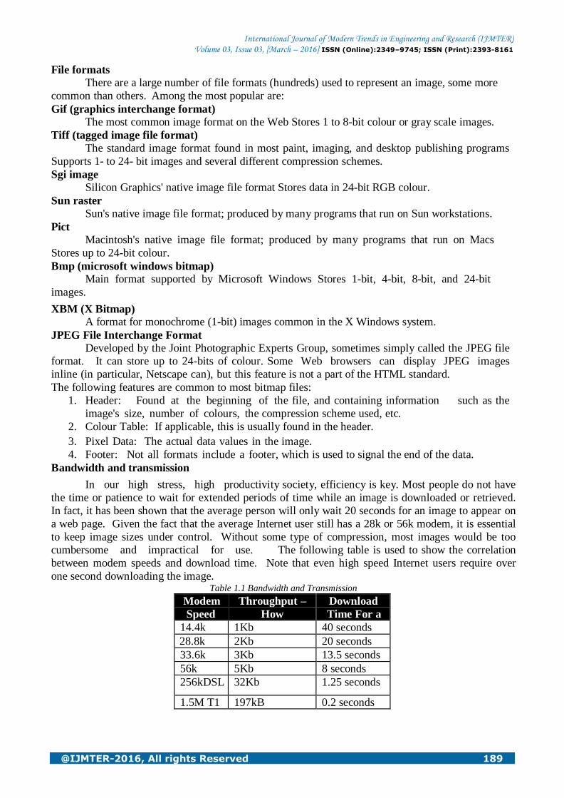
cumbersome and impractical for use. The following table is used to show the correlation

between modem speeds and download time. Note that even high speed Internet users require over

one second downloading the image. Table 1.1 Bandwidth and Transmission

Modem

Speed

Throughput –

How

Much Data

Per

Secon

d

Download

Time For a

40k Image 14.4k 1Kb 40 seconds

28.8k 2Kb 20 seconds

33.6k 3Kb 13.5 seconds

56k 5Kb 8 seconds

256kDSL 32Kb 1.25 seconds

1.5M T1 197kB 0.2 seconds



1.1 Download time comparison an introduction to image compression

Image compression is the process of reducing the amount of data required to represent a

digital image. This is done by removing all redundant or unnecessary information. An

uncompressed image requires an enormous amount of data to represent it as an example, a

standard 8.5" by 11" sheet of paper scanned at 100 dpi and restricted to black and white requires

more than 100k bytes to represent. Another example is the 276-pixel by 110-pixel banner that

appears at the top of Google.com. Uncompressed, it requires 728k of space. Image compression is

thus essential for the efficient storage, retrieval and transmission of images. In general, there are

two main categories of compression. Lossless compression involves the preservation of the image as

is (with no information and thus no detail lost).Lossy compression on the other hand, allows less

than perfect reproductions of the original image. The advantage being that, with a lossy algorithm,

one can achieve higher levels of compression because less information is needed. Various amounts

of data may be used to represent the same amount of information. Some representations may be

less efficient than others,depending on the amount of redundancy eliminated from the data. When

talking about images there are three main sources of redundant information:

1. Coding Redundancy- This refers to the binary code used to represent grey values.

2. Interpixel Redundancy- This refers to the correlation between adjacent pixels in an image.

3. Psycho visual Redundancy - This refers to the unequal sensitivity of the human eye to

different visual information.

In comparing how much compression one algorithm achieves verses another, many

people talk about a compression ratio. A higher compression ratio indicates that one algorithm

removes more redundancy then another (and thus is more efficient). If n1 and n2 are the number of

bits in two datasets that represent the same image, the relative redundancy of the first dataset is

defined as:

Rd=1/CR, where CR (the compression ratio) =n1/n2

The benefits of compression are immense. If an image is compressed at a ratio of 100:1, it

may be transmitted in one hundredth of the time, or transmitted at the same speed through a channel

of one-hundredth the bandwidth (ignoring the compression/decompression overhead). Since

images have become so commonplace and so essential to the function of computers, it is hard to see

how we would function without them.

1.2 The image compression model

Although image compression models differ in the way they compress data, there are

many general features that can be described which represent most image compression algorithms.

The source encoder is used to remove redundancy in the input image. The channel encoder is used

as overhead in order to combat channel noise.A common example of this would be the

introduction of a parity bit. By introducing this overhead, a certain level of immunity is gained

from noise that is inherent in any storage or transmission system. The channel in this model could

be either a communication link or a storage/retrieval system. The job of the channel and source

decoders is to basically undo the work of the source and channel encoders in order to restore the

image to the user.

Fidelity criterion A measure is needed in order to measure the amount of data lost (if any) due to a

compression scheme. This measure is called a fidelity criterion. There are two main categories of

fidelity criterion: subjective and objective. Objective fidelity criterion, involve a quantitative

approach to error criterion. Perhaps the most common example of this is the root mean square

error. A very much related measure is the mean square signal to noise ratio. Although objective

field criteria may be useful in analyzing the amount of error involved in a compression scheme, our

eyes do not always see things as they are which is why the second category of fidelity criterion is



important. Subjective field criteria are quality evaluations based on a human observer. These ratings

are often averaged to come up with an evaluation of a compression scheme. There are absolute

comparison scales, which are based solely on the decompressed image, and there are relative

comparison scales that involve viewing the original and decompressed images side by side in

comparison.

Table 1.2 Absolute Comparisons Scale

Value Rating Description 1 Excellent An i m a g e of ex t r em e l y high quality.

As good as desired.

2 Fine An image of high quality, providing

enjoyable viewing.

3 Passable An image of acceptable quality.

4 Marginal An image of poor quality one

Wish to improve it.

5 Inferior A very poor image, but one can see it.

6 Unusable An image so bad, one can't see it.

An obvious problem that arises is that subjective fidelity criterion may vary from person

to person. What one person sees a marginal, another may view as passable, etc.

II.PROPOSED SYSTEM

In this proposed system the new method of Curvelet Transform in blend with Lifting Scheme

and Huffman coding are used to compress iris images. In different types of wavelet transforms, the

Curvelet transform provides better results for the curvy portions of iris images. Along with

Curvelet transform, Lifting Wavelet transform is applied to the co-efficient of the Curvelet

transformed image which will provide the high detailed image. Then, after the decomposition of

iris image by Curvelet and Lifting wavelet transform, Huffman encoding is used to compress

the decomposed medical image. The reconstruction of the medical image is done by applying the

inverse lifting transform and Curvelet transform which resembles the original image exactly.

2.1Theory of Curvelet transform

2.1.1 Need for Curvelet transform

Wavelet transform is useful smooth functions in one dimension. Still Wavelet transform has

following Disadvantage Compare to Curvelet transform. 2-D line singularities - piecewise

smooth signals resembling images have 1- Dimensional Singularities. These smooth regions are

separated by edges. Normally edges are discontinuous across the image. Lack of shift invariance-

these results from the down sampling operation. Lack of directional selectivity- as the DWT filters

are real and separable the DWT cannot distinguish between the opposing diagonal directions. The

first problem of the DWT an anisotropic geometric is solved by the first order Curvelet transform

which deals with the 2-D line singularities. The second order Curvelet transform deals with the image

boundaries and it is very effective in various image processing applications. The second and third

problems of wavelet transform can be overcome by the fast discrete Curvelet transform which is

also called 2D digital Curvelet transform. In which the directional selectivity and shift invariance

is improved compare to conventional DWT.

2.2 Importance of Curvelet compare to wavelets Curvelet will be superior over wavelets in following cases:

i. This transform is optimally sparse representation of Objects with edges.



ii. This transform is optimal image reconstruction in severely ill-posed problems.

iii. This transform is optimal sparse representation of Wave Propagators.

The Curvelet represents optimal sparseness for curved punctured smooth images where the

image is smooth with the exception of discontinuity of C2 curves.

2.3 C ontinuous Curvelet transform

The first Curvelet transform used as a complex series of steps involving the Ridge let

analysis of the radon transform of an image. Performance of the Ridge let transform is very slow.

So the use of Ridge let transform was discarded and thus new method and approach to Curvelet as

tight frame is taken using tight frame, an individual Curvelet has frequency support in a parabolic

wedge area of the frequency domain.

In a heuristic argument is made that all Curvelet fall into one of three categories.

i. The Curvelet coefficient magnitude will be zero. Whose length wise support does not

intersect discontinuity?

ii. A Curvelet whose length-wise support intersects with a Discontinuity, but not at its critical

angle. At this point The Curvelet Coefficient magnitude will be close to zero.

iii. A Curvelet whose length-wise support intersects with a Discontinuity, at there the Curvelet

coefficient magnitude will be much larger than zero.

2.4 Discrete Curvelet transform The second generation Curvelet transform has two different implementations: Curvelet via

USFFT (Unequally spaced Fast Fourier transform) and frequency wrapping. Both of this Curvelet

are simpler, faster and less redundant compare to first generation Curvelet (Ridge let transform).In

this work Curvelet based on frequency wrapping technique is used.

Basically multi resolution discrete Curvelet transform have the advantage of FFT (Fast

Fourier transform).during the FFT both the image and the Curvelet at a given scale and orientation

are transformed into the Fast Fourier domain. In the spatial domain the convolution of the

Curvelet transform becomes product in their Fourier domain. Curvelet coefficients are obtained by

applying inverse FFT to the spectral product after the end of the whole computation process.

All the coefficients of the scale and orientation are in ascending order. Inverse FFT cannot be

applied on the obtained frequency spectrum because the frequency response of a Curvelet is a

trapezoidal wedge which needs to be wrapped into a rectangular support to perform the inverse

Fourier transform.The Frequency wrapping of this trapezoidal wedge which needs to be wrapped

into a rectangular support to perform the inverse Fourier domain. The wrapping of this trapezoidal

wedge is done by periodically tilting the spectrum inside the wedge and then collecting the

rectangular coefficients area in the origin. Due to this periodic tilting the rectangular region

collects the wedge’s corresponding fragmented portions from the surrounding parallelograms. For

this wedge wrapping process, this approach of Curvelet transform is known as the “wrapping

based Curvelet transform”.

Wrapping DCT Algorithm:

1. Take FFT of the Image.

2. Divide FFT into collection of Digital Tiles.

3. For each tile,

(a) Translate the tile to the origin

(b) Wrap the parallelogram shaped support of the tile around a rectangle centred at the

origin.

(c) Take the inverse FFT of the wrapped support.

(d) Add the curvelet array to the collection of curvelet coefficients.



Figure 2.1 conventional wavelet (maxican hat)

Figure 2.2 Curvelet transform

Figure 2.3 Proposed system block diagram



2.3 Proposed system block diagram modules

Step 1: In pre-processing step the wiener filter is used for removal of blur in images

due to Linear motion or unfocussed optics removes the noise.

Step 2: Pre-processed image is decomposed by discrete Curvelet transform.

Step 3: After that Integer wavelet transform is applied on the transformed image for

separating The more decorrelated coefficients.

Step4: Finally, the coefficients are encoded by Huffman encoder.

Step 5: analyze the compression ratio.

Step 6: Inverse IWT and Curvelet transform used for reconstructing the image.

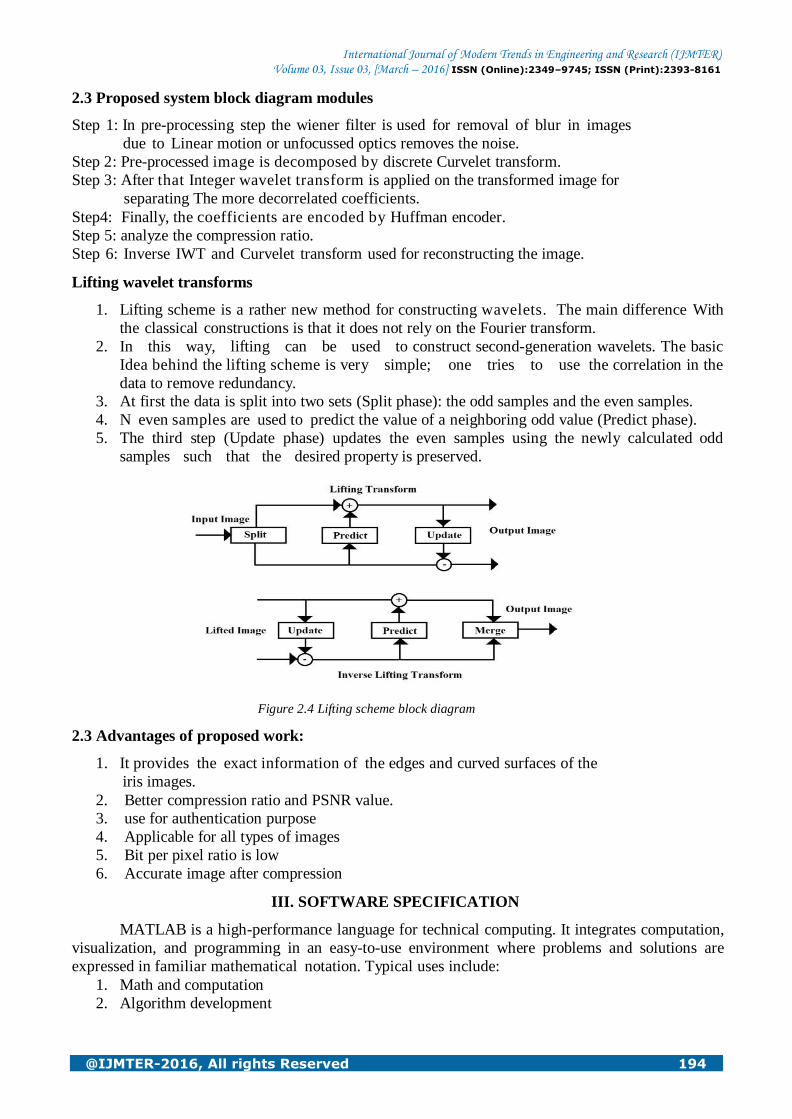
Lifting wavelet transforms

1. Lifting scheme is a rather new method for constructing wavelets. The main difference With

the classical constructions is that it does not rely on the Fourier transform.

2. In this way, lifting can be used to construct second-generation wavelets. The basic

Idea behind the lifting scheme is very simple; one tries to use the correlation in the

data to remove redundancy.

3. At first the data is split into two sets (Split phase): the odd samples and the even samples.

4. N even samples are used to predict the value of a neighboring odd value (Predict phase).

5. The third step (Update phase) updates the even samples using the newly calculated odd

samples such that the desired property is preserved.

Figure 2.4 Lifting scheme block diagram

2.3 Advantages of proposed work:

1. It provides the exact information of the edges and curved surfaces of the

iris images.

2. Better compression ratio and PSNR value.

3. use for authentication purpose

4. Applicable for all types of images

5. Bit per pixel ratio is low

6. Accurate image after compression

III. SOFTWARE SPECIFICATION

MATLAB is a high-performance language for technical computing. It integrates computation,

visualization, and programming in an easy-to-use environment where problems and solutions are

expressed in familiar mathematical notation. Typical uses include:

1. Math and computation

2. Algorithm development



3. Modeling, simulation, and prototyping

4. Data a n a l ys i s , e x p l o r a t i o n , a n d visualization

5. Scientific and engineering graphics

6. Application development, including graphical user interface building.

MATLAB is an interactive system whose basic data element is an array that does not

require dimensioning. This allows you to solve many technical computing problems, especially

those with matrix and vector formulations, in a fraction of the time it would take to write a program

in a scalar no interactive language such as C or FORTRAN.

The name MATLAB stands for matrix laboratory. MATLAB was originally written to

provide easy access to matrix software developed by the LINPACK and EISPACK projects. Today,

MATLAB uses software developed by the LAPACK and ARPACK projects, which together

represent the state-of-the-art in software for matrix computation.

MATLAB has evolved over a period of years with input from many users. In university

environments, it is the standard instructional tool for introductory and advanced courses in

mathematics, engineering, and science. In industry, MATLAB is the tool of choice for high-

productivity research, development, and analysis.

MATLAB features a family of application-specific solutions called toolboxes. Very important

to most users of MATLAB, toolboxes allow learning and applying specialized technology. Toolboxes

are comprehensive collections of MATLAB functions (M-files) that extend the MATLAB

environment to solve particular classes of problems. Areas in which toolboxes are available include

signal processing, control systems, neural networks, fuzzy logic, wavelets, simulation, and many

others.

In MATLAB, we should start by reading Manipulating Matrices. The most important

things to learn are how to enter matrices: (colon) operator, and invoke functions. At the heart of

MATLAB is a new language we must learn before we can fully exploit its power. The basics of

MATLAB can be studied quickly, and mastery comes shortly after. It can get high productivity, high-

creativity computing power that will change the way work.

Starting and quitting mat lab starting mat lab On the Microsoft Windows platform, to start MATLAB, double-click the MATLAB shortcut

icon on Windows d e s k t o p . On the U N I X platform, to start MATLAB, type MATLAB

at the operating system prompt. After starting MATLAB, the MATLAB desktop opens - see

MATLAB Desktop. It can change the directory in which MATLAB starts, define start up options

including running a script upon start up, and reduce start up time in some situations.

Quitting mat lab To end the MATLAB session, select Exit MATLAB f r o m the F i l e m e n u i n the

desktop, or type quit in the Command Window. To execute specified functions each time

MATLAB quits, such as saving the workspace, it can create and run a finish m script.

MATLAB desktop When start the MATLAB, the MATLAB desktop appears, containing tools (graphical user

interfaces) for managing files, variables, and applications associated with MATLAB.

The first time MATLAB starts, the desktop appears as shown in the following illustration,

although your launch pad may contain different entries Use the Command Window to enter

variables and run functions and M-files.



Figure 3.1 Matlab window

Features of Matlab manipulating matrices The best way for us to get started with MATLAB is to learn how to handle matrices.

Start MATLAB and follow along with each example.

It enters matrices into MATLAB in several different ways:

1. Enter an explicit list of elements.

2. Load matrices from external data files.

3. Generate matrices using built-in functions.

4. Create matrices with your own functions in M-files.

Start by entering Durer’s matrix as a list of its elements. Few basic conventions are:

1. Separate the elements of a row with blanks or commas.

2. Use a semicolon; to indicate the end of each row.

3. Surround the entire list of elements with square brackets, [ ].

To enter Durer’s matrix, simply type in the Command Window

A = [16 3 2 13; 5 10 11 8; 9 6 7 12; 4 15 14 1]

MATLAB displays the matrix you just entered.

A =16 3 2 13

5 10 11 8

9 6 7 12

4 15 14 1

This exactly matches the numbers in the engraving. Once we have entered the matrix, it is

automatically remembered in the MATLAB workspace. It refers to it simply as A.

Expressions Like most other programming languages, MATLAB provides mathematical expressions,

but unlike most programming languages, these expressions involve entire matrices.

The building blocks of expressions are:

1. Variables

2. Numbers

3. Operators

4. Functions



Variables MATLAB does not require any type declarations or dimension statements. When MATLAB

encounters a new variable name, it automatically creates the variable and allocates the appropriate

amount of storage.

If the variable already exists, MATLAB changes its contents and, if necessary, allocates new

storage. For example, num_ students =

25.Creates a 1-by-1 matrix named num_ students and stores the value 25 in its single element.

Variable names consist of a letter, followed by any number of letters, digits, or underscores.

MATLAB uses only the first 31 characters of a variable name.

MATLAB is case sensitive; it distinguishes between uppercase and lowercase letters. A and

B are not the same variable. To view the matrix assigned to any variable, simply enter the

variable name.

Numbers MATLAB uses conventional decimal notation, with an optional decimal point and leading

plus or minus sign, for numbers. Scientific notation uses the letter e to specify a power-of-ten

scale factor. Imaginary numbers use either i or j as a suffix. All numbers are stored internally using

the long format specified by the IEEE floating-point standard. Floating-point numbers have a finite

precision of roughly 16 significant decimal digits and a finite range of roughly 10-308 to

10+308.

Some of the functions, like sqrt and sin, are built-in. They are part of the MATLAB core so

they are very efficient, but the computational details are not readily accessible. Other functions, like

gamma and sinh, are implemented in M-files. We can see the code and even modify it if we

want. Several special functions provide values of useful constants.

Operators

Expressions use familiar arithmetic operators and precedence rules.

Table 3.2 Arithmetic operators and precedence rule

+ Addition

- Subtraction

* Multiplication

/ Division

\ Left division (described in "Matrices

and Linear Algebra" in Using

MATLAB)

^ Power

' Complex conjugate transpose

( ) Specify evaluation order

Functions MATLAB provides a large number of standard elementary mathematical functions,

including abs, sqrt, exp, and sin. Taking the square root or logarithm of a negative number is

not an error; the appropriate complex result is produced automatically. MATLAB also

provides many more advanced mathematical functions, including Bessel and gamma functions.

Most of these functions accept complex arguments.



Table 3.3 Functions

Pi 3.14159265...

I Imaginary unit, √-1

Eps Floating-point relative

precision, 2-52

Realmin Smallest floating-point

number, 2-1022

Realmax Largest floating-point

number, (2- ε)21023

Inf Infinity

NaN Not-a-number

List of matlab commands

1. Imread Read image from graphics file

Syntax: Imread (filename, fmt)

Description: A = Imread (filename, fmt) reads a greyscale or colour image from the file specified by

the string filename. If the file is not in the current folder, or in a folder on the MATLAB

path, specify the full pathname.

2. Imwrite: Write image to graphics file

syntax: Imwrite (A, filename, fmt)

Description: Imwrite (A, filename, fmt) writes the image A to the file specified by filename in the

format specified by fmt.

3. Imshow: Display image

Syntax: Imshow(I)

Description: imshow(I) displays the grayscale image I

4. RGB2GRAY Convert RGB image or colourmap to grayscale

Syntax: I=rgb2gray (RGB);

Description: I = rgb2gray(RGB) converts the true colour image RGB to the grayscale intensity image I.

rgb2gray converts RGB images to grayscale by eliminating the hue and saturation information

while retaining the luminance.

5. Im2double Convert image to double precision

Syntax: I2 = im2double (I)

Description:



I2 = im2double (I) converts the intensity image I to double precision, rescaling the data if

necessary. If the input image is of class double, the output image is identical.

6. Imresize Resize image

Syntax: B = imresize (A, [mrows ncols])

Description: B = imresize (A, [mrows ncols]) returns image B that has the number of rows and

columns specified by [mrows ncols]. Either NUMROWS or NUMCOLS may be NaN, in which case

imresize computes the number of rows or columns automatically to preserve the image aspect ratio.

7. Zeros Create array of all zeros

Syntax: B=zeros (n) B = zeros(m,n)

Description: B = zeros (n) returns an n-by-n matrix of zeros. An error message appears if n is not a

scalar.

8. Max Largest elements in array

Syntax: C=max(A) C=max (A,B) C=max (A,[],dim) [C,I] = max (...)

Description: C = max (A) returns the largest elements along different dimensions of an array.

If A is a vector, max (A) returns the largest element in A.

If A is a matrix, max (A) treats the columns of A as vectors, returning a row vector

containing the maximum element from each column.

If A is a multidimensional array, max (A) treats the values along the first non-singleton

dimension as vectors, returning the maximum value of each vector.

C = max (A, B) returns an array the same size as A and B with the largest elements taken

from A or B. The dimensions of A and B must match, or they may be scalar.

C = max (A, [], dim) returns the largest elements along the dimension of A specified by

scalar dim. For example, max (A, [], 1) produces the maximum values along the first dimension

(the rows) of A.

[C, I] = max (...) finds the indices of the maximum values of A, and returns them in output

vector I. If there are several identical maximum values, the index of the first one found is

returned.

B = zeros (m, n) or B = zeros ([m n]) returns an m-by-n matrix of zeros.

9. Min Smallest elements in array

Syntax:

C=min(A) C=min(A,B) C=min(A,[],dim) [C,I] = min(...)

Description: C = min (A) returns the smallest elements along different dimensions of an array.

If A is a vector, min (A) returns the smallest element in A.

If A is a matrix, min (A) treats the columns of A as vectors, returning a row vector

containing the minimum element from each column.

If A is a multidimensional array, min operates along the first nonsingleton dimension.

C = min (A, B) returns an array the same size as A and B with the smallest elements taken

from A or B. The dimensions of A and B must match, or they may be scalar.



C = min (A, [], dim) returns the smallest elements along the dimension of A specified by

scalar dim. For example, min (A, [], 1) produces the minimum values along the first dimension

(the rows) of A.

[C, I] = min (...) finds the indices of the minimum values of A, and returns them in output

vector I. If there are several identical minimum values, the index of the first one found is returned.

IV.CONCLUSION

The bit rate required for visually lossless compression of 3D monochrome stereo pairs is

larger than that required for visually lossless 2D compression of the individual left and right

images. However, the resulting left and right images Obtained v i a t h e e x i s t i n g m e t h o d a r e

v i s u a l l y lossless in both 2D and 3D mode, while the images compressed individually are not

visually lossless in 3D mode. The existing method results in a significantly higher bit rate

than proposed scheme. I will use for authentication purpose and applicable for 2D images also.

Compression ratio is to be high when comparing to existing system.

REFERENCES

[1] P. Dal Poz, R. A. B. Gallis, J. F. C. da Silva, and E. F. O. Martins, “Object-space road extraction in rural areas using

stereoscopic aerial images,” IEEE Geosci. Remote Sens. Lett, vol. 9, no. 2, pp. 654–658, Jul. 2012.

[2] D. P. Noonan, P. Mountney, D. S. Elson, A. Darzi, and G.-Z. Yang, “A stereoscopic fibroscope for camera motion

and 3D depth recovery during minimally invasive surgery,” in Proc. IEEE Int. Conf. Robot. Autom., Kobe,

Japan, May 2009, pp. 4463–4468.

[3] L. Lipton, “The stereoscopic cinema: From film to digital projection,” SMPTE J., pp. 586–593, Sep.2001.

[4] D. A. Bowman, 3D User Interfaces: Theory and Practice. Boston, MA, USA: Addison-Wesley,2005.

[5] S. Pastoor and M. Wöpking, “3D displays: A review of current technologies,” Displays, vol. 17, no. 2, pp. 100–110,

Apr. 1997.

[6] H. Urey, K. V. Chellappan, E. Erden, and P.Surman, “State of the art in stereoscopic and autostereoscopic

displays,” Proc. IEEE, vol. 99, no. 4, pp. 540–555, Apr. 2011.

[7] M. Barkowsky, S. Tourancheau, K. Brunnström, K. Wang, and B. Andrén, “Crosstalk measurements of shutter

glasses 3D displays,” in Proc. SID Int. Symp., 2011, pp. 812–815.

an improved image compression using … · the most common image format on the web stores 1 to...

Documents