An Introduction to HyperSpy:The multi-dimensional data analysis toolbox

Josh Taillon and Andy Herzing

April 5, 2018

A quick note rst:

This isn't your parents' Powerpoint...

...because everything is interactive!

In [3]:

Today is April 05, 2018!

import datetimeimport timedatestring = datetime.datetime.now().strftime('%B %d, %Y')for c in 'Today is {}!'.format(datestring): print(c, end='') time.sleep(.1)

Made possible with:

Jupyter notebook — https://jupyter.org/

RISE (Reveal.js IPython/Jupyter Slideshow Extension) — https://github.com/damianavila/RISE

2 . 4

Introduction

3 . 1

What is HyperSpy?

Open-source Python library for interactive data analysis of multi-dimensional datasets

Makes it easy to operate on multi-dimensional arrays as you would a single spectrum (or image)

Easy access to cutting-edge signal processing tools

Modular structure makes it easy to add custom features

4 . 1

Why   ?

4 . 2

Why   ?

Quickly becoming the de facto standard of scienti c computing

Free (as in speech and as in beer)

No pesky licenses to checkout

Vast array of scienti c libraries available:

pip install antigravity

Thanks to numpy and other libraries, similar (or often better) performance than MATLAB

History of HyperSpy

Developed by in 2007 — 2012 as part of Ph.D. ThesisFrancisco de la Peña

Originally called EELSLab:

Open-sourced (on ) in 2010Github

Renamed to HyperSpy in 2011

Now... over 100 citations, and rapidly growing!

4 . 5

Design philosophy of HyperSpy

HyperSpy is a Python library, rather than standalone program

Part of the greater scienti c Python ecosystem

Data storage is in an open hierarchical format (HDF5)

Analysis done via reproducible notebooks

Feature development is completely open-source

5 . 1

How we came to love HyperSpy

6 . 1

Josh:

Became interested in multivariate statistical analysis of EELS spectrum images

No easy way to do that in commercial software

The entire scienti c Python ecosystem is available from HyperSpy —

machine learning, clustering, signal separation, etc.

Came for the data analysis, stayed because of the community

6 . 2

Andy:

Needed a way to ef ciently and objectively process chemical tomography data based on

hyperspectral images

No available commercial options except brute force

Quickly realized that HyperSpy was ideally set up to enable reproducible and well documented data

analysis

You know, science!

6 . 3

Getting Started

6 . 4

Installation

Easiest method on Windows — HyperSpy bundle

Installs a Python distribution with HyperSpy included

Best method if you have no prior Python experience

http://hyperspy.org/download.html#windows-bundle-installers

For more control (on Windows, Mac, and Linux) — Anaconda Python

After installing Anaconda, simply run conda install hyperspy

This method is preferred by the developers

https://www.anaconda.com/download/

7 . 1

How to use HyperSpy?

Console/Command line

Integrated development environment (IDE)

Jupyter Notebook (and JupyterLab)

HyperSpyUI

Important note:

Because HyperSpy is a library, all of these are just generic ways to access Python, and not speci c to HyperSpy! (except the last one)

Console/Command line

The simplest way to run is with a pre-written script directly from the command line:

$ python analysis_script.py

There are also "advanced Python interpreters", such as Jupyter QTConsole, bpython , ipython , etc.

Integrated Development Environments

Spyder (live example)

PyCharm

NetBeans

Jupyter Notebook

The Jupyter project ( ) exists to:

"...develop open-source software, open-standards, and services for interactive computing across dozens ofprogramming languages."

https://jupyter.org

The "Notebook" is a human-readable format for storing both the inputs and outputs of code (see)...

Inspired by Mathematica and Maple; has been adopted in many languages

https://en.wikipedia.org/wiki/Notebook_interface

8 . 6

Features of the notebook:

Separation of the kernel (for calculation) and the front-end (for display)

Runs completely in the web-browser (no special software needed)

Kernel can be run on a central server — users connect with a web browser

.ipynb les are JSON format and can be versioned

Language-agnostic (can be used with Python, R, Java, Julia, etc.)

8 . 7

Jupyter Lab

An exciting new project that is more fully-featured and will eventually replace the Notebook interface

Aims to be an IDE like Spyder or RStudio, but running within the browser

Incorporates notebooks, the terminal, text editor, le browser, rich outputs, etc. into one interface

8 . 8

HyperSpyUI ( )https://github.com/hyperspy/hyperspyui

Developed in parallel to HyperSpy as a more "user-friendly" experience

Many commonly used features from HyperSpy are available

Deviation for a short view of HyperSpyUI (loading EELS signal, view metadata, signal separation,

macro recorder)

Most use Jupyter notebooks, but the UI is useful for quick investigations, or for those without

programming experience

8 . 9

How to get help?

Well-documented user guide and documentation: http://hyperspy.org/hyperspy-

doc/current/user_guide/index.html

Tutorials and demos: https://github.com/hyperspy/hyperspy-demos

User group list: hyperspy-users@googlegroups.com

Gitter chat: https://gitter.im/hyperspy/hyperspy

If all else fails, Andy and Josh

9 . 1

HyperSpy's Signal Class

The "heart" of HyperSpy's data structure

Every dataset stored within HyperSpy is a sub-class of Signal

10 . 1

Structure of a Signal

Signal is a wrapper around the raw data

Data is stored in a numpy array

Calibration information is stored in two types of Axes objects:

Navigation and Signal dimensions

In [4]:

Out[4]:< Axes manager, axes: (20, 10|30) >

Navigation axis name size index offset scale units

20 0 0.0 1.0

10 0 0.0 1.0

Signal axis name size offset scale units

30 0.0 1.0

hs.signals.Signal1D(np.random.random((10, 20, 30))).axes_manager

10 . 2

Structure of a Signal

Examples of signal dimensionality:

Navigation Signal

Single spectrum 0 1

Line scan spectrum image 1 1

Areal spectrum image 2 1

Single image 0 2

Time series image stack 1 2

4D STEM diffraction image 2 2

10 . 3

Structure of a Signal

Signals can be sliced by index, or by axis units, on either type of axis

Signal axis slicing:

In [5]:

<EDSSEMSpectrum, title: EDS SEM Spectrum, dimensions: (|1024)> <EDSSEMSpectrum, title: EDS SEM Spectrum, dimensions: (|400)> <EDSSEMSpectrum, title: EDS SEM Spectrum, dimensions: (|80)>

s = hs.datasets.example_signals.EDS_SEM_Spectrum()print(s) # Slice by axis units with floats:print(s.isig[1.0:5.0]) # Slice by index with integers:print(s.isig[20:100])

10 . 4

Navigation axis slicing:

In [6]:

<Signal2D, title: 03_5Mx_scale_corrected, dimensions: (|512, 512)> <Signal2D, title: 03_5Mx_scale_corrected, dimensions: (|83, 40)>

im = hs.load('examples/HRSTEM.dm3')print(im) # Slice by axis units and index:im_crop = im.isig[1.0:10.5, 20:60]print(im_crop)im_crop.plot()

10 . 5

Getting your data in (and out) of HyperSpy

Many data readers have been written for experimental tools:

11 . 2

Loading data is simple!

Example of Gatan's dm3 format:

In [7]:

In [8]:

In [9]:

Out[8]: <Signal2D, title: 03_5Mx_scale_corrected, dimensions: (|512, 512)>

Out[9]: ├── Acquisition_instrument │ └── TEM │ ├── acquisition_mode = STEM │ ├── beam_current = 0.0 │ ├── beam_energy = 200.0 │ ├── camera_length = 20.0 │ ├── dwell_time = 0.00012989999389648437 │ ├── magnification = 5000000.0 │ └── microscope = JEOL COM ├── General │ ├── date = 2016-05-07 │ ├── original_filename = HRSTEM.dm3 │ ├── time = 12:58:18 │ └── title = 03_5Mx_scale_corrected └── Signal ├── Noise_properties │ └── Variance_linear_model │ ├── gain_factor = 1.0 │ └── gain_offset = 0.0 ├── binned = False ├── quantity = Intensity └── signal_type =

im = hs.load('examples/HRSTEM.dm3')

im

im.metadata

Original metadata is maintained:

In [10]:

Out[10]: ├── ApplicationBounds = (0, 0, 984, 1920) ├── DocumentObjectList │ └── TagGroup0 │ ├── AnnotationGroupList │ │ └── TagGroup0 │ │ ├── AnnotationType = 31 │ │ ├── BackgroundColor = (0, 0, 0) │ │ ├── BackgroundMode = 2 │ │ ├── FillMode = 2 │ │ ├── Font │ │ │ ├── Attributes = 0 │ │ │ ├── FamilyName = Microsoft Sans Serif │ │ │ └── Size = 7 │ │ ├── ForegroundColor = (-1, -1, -1) │ │ ├── HasBackground = 0 │ │ ├── IsMoveable = 1 │ │ ├── IsResizable = 1 │ │ ├── IsSelectable = 1 │ │ ├── IsTranslatable = 1 │ │ ├── IsVisible = 1 │ │ ├── ObjectTags │ │ ├── Rectangle = (482.0, 16.0, 496.0, 142.0)

im.original_metadata

11 . 4

Plotting is also simple within the notebook:

In [11]: im.plot()

11 . 5

EDAX EDS mapping data

In [12]:

In [13]:

In [14]:

Out[13]: <EDSSEMSpectrum, title: EDS Spectrum Image, dimensions: (256, 231|2000)>

Out[14]:

< Axes manager, axes: (256, 231|2000) >

Navigation axis name size index offset scale units

x 256 0 0.0 0.02440594509243965

y 231 0 0.0 0.022832725197076797

Signal axis name size offset scale units

Energy 2000 0.0 0.005 keV

μm

μm

s = hs.load('examples/SEM_EDS_map.spd')

s

s.axes_manager

11 . 6

In [15]: s.plot()

11 . 7

In [16]: sbin = s.rebin(new_shape=[64, 56, 500])sbin.plot()

11 . 8

Generic data access

A Signal can be created from any data that can be expressed as a numpy array

If your tool can output raw data, it can be loaded into HyperSpy with little fuss

Using general Python features, data from other sources can be loaded easily as well

Loading a .csv spectrum le

In [17]:

# Energy (eV), Counts 9.000000134110450745e+01,1.090600000000000000e+04 9.020000134408473969e+01,1.090400000000000000e+04 9.040000134706497192e+01,1.069800000000000000e+04 9.060000135004520416e+01,1.044400000000000000e+04 9.080000135302543640e+01,1.038000000000000000e+04 9.100000135600566864e+01,1.030400000000000000e+04 9.120000135898590088e+01,1.019400000000000000e+04 9.140000136196613312e+01,1.022700000000000000e+04 9.160000136494636536e+01,1.006700000000000000e+04

# Print the first few lines of the .csv file for inspection:with open('examples/spectrum.csv', 'r') as f: for i in range(10): print(f.readline(), end='')

12 . 2

In [18]:

In [19]:

Out[18]: <Signal1D, title: , dimensions: (|2041)>

Out[19]:

< Axes manager, axes: (|2041) >

Signal axis name size offset scale units

Energy 2041 90.00000134110451 0.20000000298023224 eV

# Load the data into a numpy array from the .csv file:d = np.loadtxt("examples/spectrum.csv", delimiter=',') # Create a signal from the second column of data (the spectral counts)s = hs.signals.Signal1D(d[:,1])s

# Take the first column of values and set the energy axis accordingly:energy_data = d[:,0]s.axes_manager[0].scale = np.diff(energy_data).mean()s.axes_manager[0].units = 'eV's.axes_manager[0].offset = energy_data[0]s.axes_manager[0].name = 'Energy's.axes_manager

12 . 3

In [21]: s.plot()

12 . 4

Loading and saving MATLAB les

The SciPy project provides a Matlab reader and saver that makes this easy:

In [22]:

In [23]:

b'MATLAB 5.0 MAT-file, Platform: PCWIN64, Created on: Mon Sep 11 14:27:46 2017'

Out[23]:< Axes manager, axes: (|256, 256) >

Signal axis name size offset scale units

256 0.0 1.0

256 0.0 1.0

├── General │ └── title = └── Signal ├── binned = False └── signal_type =

from scipy.io import loadmat, savemathouse = loadmat('examples/house_image.mat')print(house['__header__'])

s = hs.signals.Signal2D(house['IMin0'])print(s.metadata)s.axes_manager

12 . 5

In [24]: s.plot()

12 . 6

"Lazy" signal access

HyperSpy makes it easy to work with big data (bigger than your system's memory)

Uses the excellent library for chunking operationsdask

Almost all the regular features of HyperSpy can operate on "lazy" signals (see )User Guide

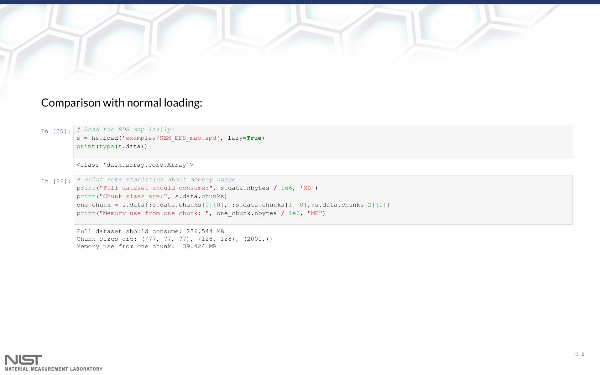
Comparison with normal loading:

In [25]:

In [26]:

<class 'dask.array.core.Array'>

Full dataset should consume: 236.544 MB Chunk sizes are: ((77, 77, 77), (128, 128), (2000,)) Memory use from one chunk: 39.424 MB

# Load the EDS map lazily:s = hs.load('examples/SEM_EDS_map.spd', lazy=True)print(type(s.data))

# Print some statistics about memory usageprint("Full dataset should consume:", s.data.nbytes / 1e6, 'MB')print("Chunk sizes are:", s.data.chunks)one_chunk = s.data[:s.data.chunks[0][0], :s.data.chunks[1][0],:s.data.chunks[2][0]]print("Memory use from one chunk: ", one_chunk.nbytes / 1e6, "MB")

13 . 2

Saving data from HyperSpy — HDF5

The default format for HyperSpy data is an .hspy le in formatHDF5

Open, hierarchical data format supporting compression and full read/write capability

All HyperSpy signals can be saved as .hspy les

Saves full metadata about signal, including critical processing parameters

Modeling, signal separation, elemental information

Saving data from HyperSpy — data interchange

Other formats can be easily written:

Single spectra — .msa format

Images — TIFF, JPG, etc.

Spectrum images — Lispix-style .rpl/.raw pairs

14 . 2

Electron microscopy-speci c tools

HyperSpy is incredibly exible, but was developed from a microscopy perspective

Has in-depth features related to image, EDS, and EELS processing

Many of the tools are applicable to multiple modalities

Some other EM tools available:

Dielectric function analysis (for plasmon EELS)

Electron holography

"Extension" projects that build upon HyperSpy (like Andy's tomotools )

Provides a robust framework on which to develop new processing pipelines

15 . 1

EDS Processing

EDS support is implemented as EDSSpectrum , a subclass of Signal for EDS-speci c features

Open metadata structure holds relevant info about instrument and detectors:

In [27]:

Also holds all the compositional information:

In [28]:

Out[27]: └── EDS ├── azimuth_angle = 0.0 ├── detector = Super-X 4 detectors Brucker ├── elevation_angle = 22.0 └── energy_resolution_MnKa = 133.312296

['Fe' 'Pt'] ['Cu', 'Fe', 'Pt']

s = hs.datasets.example_signals.EDS_TEM_Spectrum()s.metadata.Acquisition_instrument.TEM.Detector

print(s.metadata.Sample.elements) # Elements can be added easily:s.add_elements(['Cu'])print(s.metadata.Sample.elements)

16 . 1

Processing tools

All the "basic" EDS processing tools are included:

Background removal

Net intensity line map extraction

Quanti cation using Cliff-Lorimer (k-factors), -factors, and ionization cross sectionsζ

Can also use the general HyperSpy tools for more advanced analysis:

Curve tting

Machine learning

Factor reduction

Signal separation ("phase mapping")

Look to the extensive documentation in the and for helpUser Guide Tutorials

16 . 2

EELS Processing

EELS is a " rst-class citizen" — software was originally called "EELSLab"

EELS support is implemented as EELSSpectrum , a subclass of Signal for EELS-speci c features

Like EDS, open metadata structure holds relevant info about instrument and detectors:

In [29]:

Out[29]: └── TEM ├── Detector │ └── EELS │ └── collection_angle = 20.829999923706055 ├── beam_energy = 200.0 ├── convergence_angle = 12.0 └── dwell_time = 0.20000000000000001

s = hs.load('examples/signal_separation_EELS_SI.hdf5')s.metadata.Acquisition_instrument

17 . 1

Processing tools

Almost all of Egerton's EELS methods are built in:

Core-loss background subtraction

Estimating thickness

Low-loss deconvolution

Estimating elastic scattering threshold

Kramers-Kronig analysis

Can also use the general HyperSpy tools for more advanced analysis:

Curve tting

Machine learning

Factor reduction

Signal separation ("phase mapping")

Look to the extensive documentation in the and for helpUser Guide Tutorials

17 . 2

Extensibility of HyperSpy

For most, HyperSpy already does everything a microscopist might need

Open framework means if it doesn't, you can make it so!

Some examples:

Andy's tomotools

— Pythonic Crystallographic Electron Microscopy

— Quantifying atomic columns in ADF STEM images

— Fast Pixelated Detector processing

pyXem

Atomap

fpd_data_processing

18 . 1

Interactive demos

(and it's application to EELS spectrum images)Curve tting

(including source separation)Processing TEM EDS data

Extensibility (Andy's tomotools package)

19 . 1