AN INNOVATIVE WIRELESS SENSOR BASED VITAL TRAIN DETECTION AND WARNING SYSTEM

Ahtasham Ashraf*, David Baldwin and Xin Zhou Central Signal, LLC

2912 Syene Rd, Madison, WI 53713 Tel: (608) 237 1780, Fax: (608) 237 1817

{aashraf, dbaldwin, xzhou}@centralsig.com *corresponding author, Total 5816 words

ABSTRACT Adapting innovative and novel technologies for vital, fail-safe and reliable operation in a railroad

environment requires selecting a technology that is well suited to the purpose. Developing

methods to assure vital operation is equally important. Central Signal has developed a method of

vitally detecting trains using anisotropic magneto-resistive (AMR) sensors, low power spread

spectrum radios, and a central vital processing unit all powered by photo-voltaic/battery power

systems. The proposed low-cost, power-efficient wireless sensors process multi-dimensional

AMR sensor waveform data to generate a unique train signature and provide vital train detection.

This train detection and signature identification by multiple wireless sensor nodes distributed

within range of a railroad track provides the basis for a vital train detection system. A Vital

Processing Device communicates with these wireless sensors and provides an output signal

consistent with conditional state of the train detection zone. Time defined sensor polling, of

paired sensors assure a reliable and vital system that will revert to safest condition should any

element or device fail to perform it intended function. The detection method includes a unique

application of Dynamic Time Warping (DTW) method for matching the essential features of a

train signature. This train detection and signature identification by multiple wireless sensors

provides the basis for a vital train detection system.

1. INTRODUCTION AND BACKGROUND

Train detection is the fundamental task of any railroad signal system. Acceptable methods for

accomplishing this essential task must be based on designs that guarantee a train occupying a

detection zone will be detected. A corollary requirement is in the event that any element

necessary to the detection of a train fails to perform its intended function, the train detection

device must revert to safest condition. Signal engineers call devices that incorporate these

design requirements “vital” devices and describe them as “fail-safe” meaning, literally, that these

devices become safe when they fail. “Safe” means that the device reverts to its most restrictive

condition. The Federal Railroad Administration requires that all vital circuits be designed on the

closed circuit principle (1).

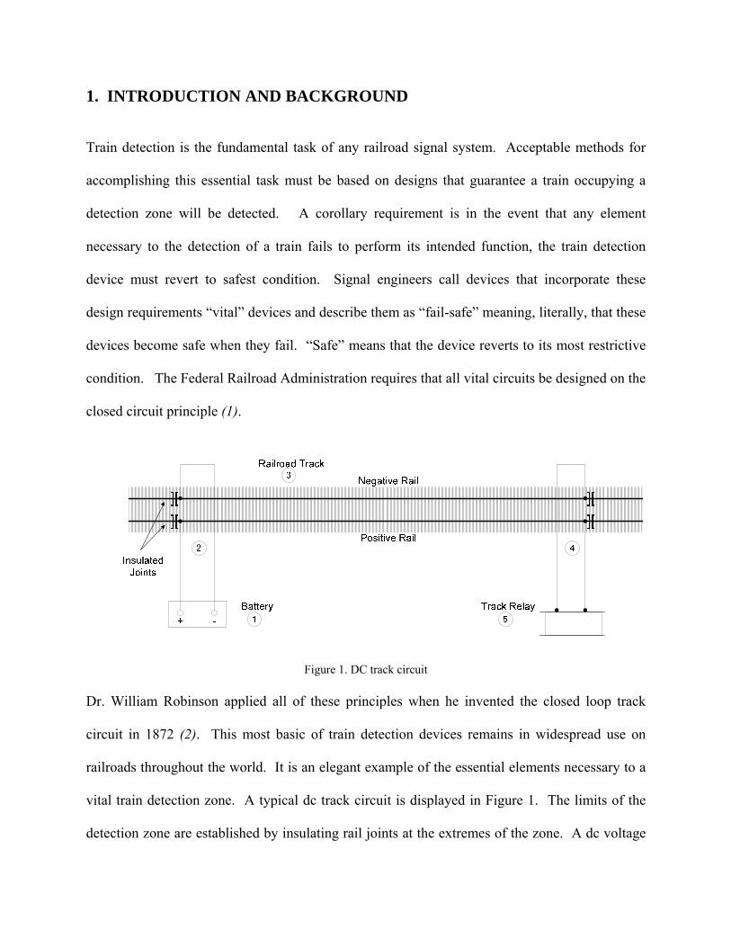
Figure 1. DC track circuit Dr. William Robinson applied all of these principles when he invented the closed loop track

circuit in 1872 (2). This most basic of train detection devices remains in widespread use on

railroads throughout the world. It is an elegant example of the essential elements necessary to a

vital train detection zone. A typical dc track circuit is displayed in Figure 1. The limits of the

detection zone are established by insulating rail joints at the extremes of the zone. A dc voltage

is connected to the track rails at one end of the zone and a dc relay is connected to the track rails

at the other end of the zone. A dc current will flow through the positive rail, through the relay

coil and return to the dc voltage source through the negative rail. This is a closed loop or closed

circuit design. The elements of the detection zone are: 1) the voltage source, 2) the connection to

the track rails, 3) each track rail, 4) connections from the track rails to the relay coil, and 5) the

track relay coil. In this series dc circuit, every element of the closed loop must function as

intended for current to flow through the track relay coil. If this track circuit is functioning as

designed, the track relay will be energized or “up” and the heel-front contacts of the relay will be

closed. The design of the track relay is a subcomponent of the track circuit and is subject to vital

design requirements as well. The electromechanical design of the relay is based upon the

requirement that if current is not flowing through the relay coil, the relay contacts will be

“down”, i.e. the heel-front relay contacts will be open. When a train occupies the track circuit,

the wheels and axles of the train provide alternate current paths of less resistance than the relay

coil. Most of the current available from the dc voltage source flows through the trains wheels

and axles leaving inadequate current to energize the track relay. The relay contacts are “down”

indicating that a train occupies the circuit. The Federal Railroad Administration requires that a

track circuit relay must be “in its most restrictive state,” i.e. in this example, “down,” when, “a

0.06 ohm resistive shunt is connected across the track rails of the circuit” (3). Notice that the

most restrictive state of the track relay is de-energized or “down” and that, by design, a properly

adjusted track circuit is down whenever it is occupied by a train or if any of the five elements of

the circuit fail to function as intended. Broken wires, broken rail (or rail bonding failures),

failure of voltage source, or relay coil faults will all result in a de-energized or “down” relay.

There are several variations of the dc track circuit, including type ac/dc, type ac feeding an ac

relay coil, coded dc or ac current sources and matching relays and numerous electronic and solid

state variations used throughout the world including audio frequency transmitter/receiver

combinations that eliminate the need to insulate rail joints to define circuit limits. In the 1950s

Stanford Research, at the request of Southern Pacific Company, developed a constant warning

device for at-grade crossing signal control. Constant warning devices and similar motion

sensitive devices transmit an audio frequency into a rail detection zone defined by shunts

connected between the track rails at the detection zone outer limits. The amplitude difference

and phase shift of audio frequency signals are detected by the device’s receiver to determine

status of the detection zone. The track zone presents a primarily inductive load to the transmitted

signal and is tuned upon installation of the device to a “normal” level that corresponds to an un-

occupied track. A failure of track connections or of the rail or of the termination will “detune”

the device. This deviation from normal will cause the device to revert to its most restrictive

state. When a train enters the “normalized” detection zone, the wheels and axles provide a

rolling or moving shunt to the audio frequency signal effectively changing the impedance of the

track detection zone. The amplitude and phase of the audio frequency as detected by the receiver

correlates with the dynamic impedance load resulting from a moving train within the track zone.

Amplitude and phase data is processed according to defined algorithms to determine if a detected

train is moving toward or away from the transmitter/receiver and speed of movement (including

detection of no movement or a standing train within the zone). Constant warning devices utilize

additional algorithms to determine speed, distance, and probable time of arrival of a train moving

toward a crossing. These state-of-the-art, very sophisticated devices are the preferred detection

system for modern grade crossing signal systems. Through several generations of devices,

railroad signal designers have resolved issues related to the use of microprocessor based systems

to provide vital railroad signal functions.

Today, all viable train detection devices and systems include a rail component necessary to vital

operation. All of the devices from dc track circuits to constant warning devices are vital. When

properly installed and adjusted, they detect trains occupying the detection zone and they revert to

most restrictive condition when the essential elements of the system are disarranged or fail.

They are excellent tools in the signal engineer’s kit but they are not perfect. Maintaining

electrical continuity of track rails, insulated rail joints, insulated track switch appliances and

device wiring connections to track rails requires continuous and constant effort. The devices are

designed to exacting standards, electronic devices are heavily redundant to increase reliability

and their cost reflects this. Most of the devices are not power efficient. System design changes

or upgrades frequently require field rewiring or full replacement. All of the devices are

susceptible to rail and ballast conditions including weather variations. Rusty or contaminated

rail may interfere with reliable or consistent detection of trains within the device’s detection

zone, the most egregious error possible for any train detection device. Contaminated track

ballast may provide sufficient alternative current paths between track rails to cause all of these

devices to revert to most restrictive condition until the contamination is resolved. None of these

devices function reliably if the track rails are under water. Northern latitude grade crossing

roadways are frequently treated with snow and ice melting agents during the winter months. It

is not unusual for de-icing contamination of the roadway or “island” train detection zone to

interfere and sometimes to prevent the proper operation of track based train detection devices.

There are a variety of innovative and novel technologies recently available that have been

suggested as additional productive tools for signal engineering vital train detection systems. The

final consideration is the cost of the vitally configured technology. The best new technology

choices will have excellent train detection characteristics, will be readily configurable as a vital

device or as an element of a vital system, will be fully compatible with current signal technology

and will cost less than technology currently in use. Various magnetometer configurations have

been explored by a number of companies searching for innovative train detection solutions.

None of those efforts have succeeded in discovering a vital design solution.

There are two types of low field magnetic sensors: 1) Coils and 2) Magneto-resistive bridges.

Coils, such as magneto-inductive and flux-gate sensors, require active oscillator circuits to detect

magnetic flux changes. Two types of magneto-resistive sensors are currently available: 1) Giant

Magneto-Resistive (GMR) and 2) Anisotropic Magneto-Resistive (AMR). GMR sensors require

a magnetic bias field to achieve the linearity necessary to train detection.

AMR sensors provide a directional one dimensional response to magnetic fields in their

magnetic sensitive axis and bridge voltage amplitude correlates linearly with field strength.

AMR elements may be combined and oriented to provide two dimensional and three dimensional

measurements. AMR devices manufactured by Honeywell, “have patented coils interleaved with

the bridge elements” (4) that can be used to offset element response to magnetic fields or to reset

magnetic domains of the sensor elements. These features are useful for eliminating temperature

drift and for compensating exposures to large magnetic fields generated by rail cars and

locomotives. AMR sensors have been evaluated for vehicle detection applications in general (4)

(5) and to train detection (4) (5) (6). Between 2002 and 2005, Central Signal deployed and

tested a magneto-inductive coil sensor, concluding that the electrical engineering necessary to

adapt this sensor type to the requirements of a vital train detection system were significant. It

was also apparent that coil type sensors lacked sufficient sensitivity to support the requirements

of a vital train detection device. Central Signal began a research and development effort in 2005

using the AMR sensor as the sensing element for train detection. Beginning in 2005, several

AMR sensor types and configurations have been deployed for extensive periods at a test site

provided by the Wisconsin & Southern Railroad at its Johnson St yard facility in Madison, WI.

2. MAGNETIC TRAIN DETECTION SYSTEM

AMR sensors have been demonstrated to reliably detect railroad trains, engines, and individual

cars at distances exceeding 60 feet. The fact that sensor output signals are affected by trains is

not, however, sufficient to vital detection. Track rail based detection schemes provide

continuous coverage of the detection zone and occupancy of the zone by a train is sampled

continuously from the time that the train enters the zone until the time that the train leaves the

zone. Discrete sensor schemes, whether they are wheel counters, vibration sensors, acoustic

detectors, photo detectors, or magnetometers cannot provide vital train detection by relying on

leading edge or leading/trailing edge detection unless the sensor distribution density

approximates continuous detection throughout the detection zone. This approximation is

invariably cost prohibitive and in actual practice may be extremely difficult to achieve.

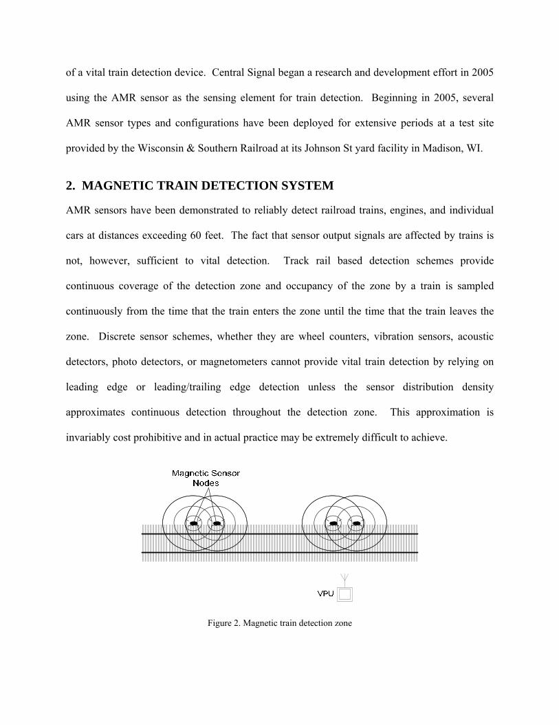
Figure 2. Magnetic train detection zone

Central Signal has invented a method to deploy AMR sensors to vitally detect trains occupying

the zone (Figure 2). The ARM sensors are one element of a sensor node configuration that

converts the analog waveform data produced by one or more AMR bridges to digital data that is

delivered to a microprocessor for analysis and evaluation. The microprocessor generates a

Unique Train Identification Signature (UTIS) that is time stamped and sent to an on-board spread

spectrum data radio that transmits the UTIS to a Vital Processing Unit (VPU). The VPU

controls other vital signal devices through its vital I/O. The VPU output is HI for unoccupied

track zones and all sensors reporting normal status within specified time frames. When a train

enters the range of a sensor, the magnitude of the AMR sensor response is evaluated. If the

required threshold is satisfied, the sensor node transmits a detection notice to the VPU which

then changes its output to LO. The sensor continues to evaluate the waveform generated by the

train event. If the train stops within range of the sensor node, that data is transmitted to the VPU.

The VPU evaluates data from this sensor node and compares data from all other sensor nodes to

determine actual train movement. If other sensor nodes report a stopped train, the VPU will

change output to HI after a delay based upon predicted location of leading edge of train at time

stop is confirmed by all sensor nodes within range of train. A continuous train movement

through the detection zone will generate at least one UTIS from two different sensor nodes as it

enters the detection zone and at least one UTIS from two different sensor nodes as it leaves the

detection zone. All UTIS must match for the VPU to conclude that the detection zone is

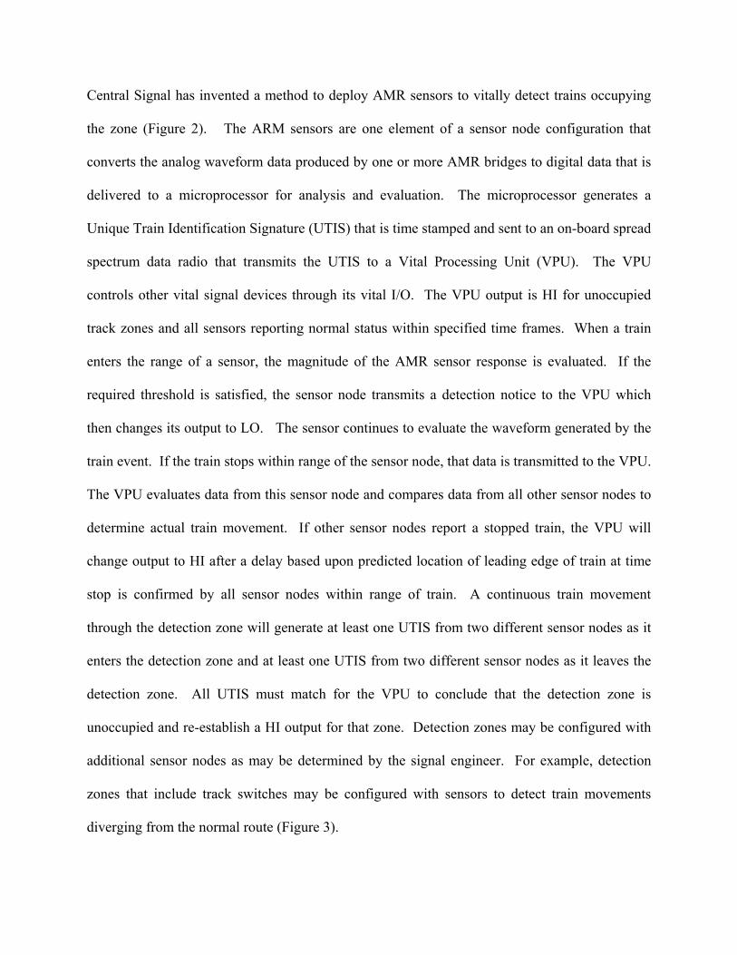
unoccupied and re-establish a HI output for that zone. Detection zones may be configured with

additional sensor nodes as may be determined by the signal engineer. For example, detection

zones that include track switches may be configured with sensors to detect train movements

diverging from the normal route (Figure 3).

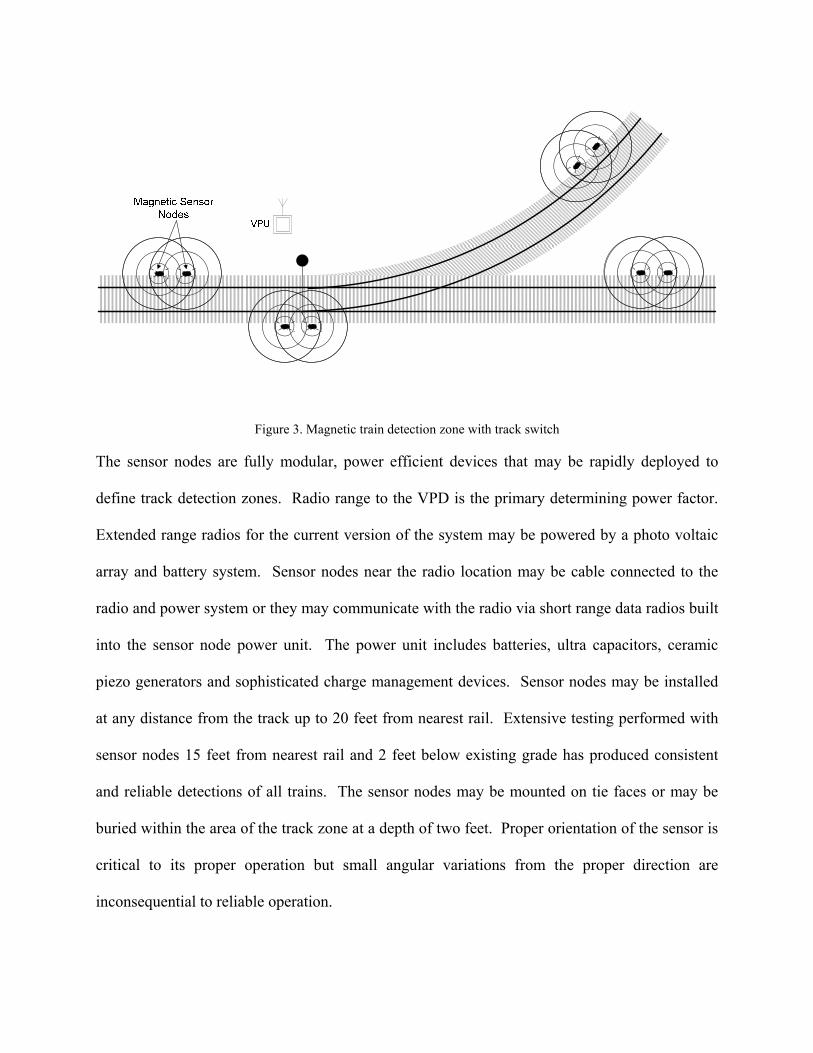
Figure 3. Magnetic train detection zone with track switch

The sensor nodes are fully modular, power efficient devices that may be rapidly deployed to

define track detection zones. Radio range to the VPD is the primary determining power factor.

Extended range radios for the current version of the system may be powered by a photo voltaic

array and battery system. Sensor nodes near the radio location may be cable connected to the

radio and power system or they may communicate with the radio via short range data radios built

into the sensor node power unit. The power unit includes batteries, ultra capacitors, ceramic

piezo generators and sophisticated charge management devices. Sensor nodes may be installed

at any distance from the track up to 20 feet from nearest rail. Extensive testing performed with

sensor nodes 15 feet from nearest rail and 2 feet below existing grade has produced consistent

and reliable detections of all trains. The sensor nodes may be mounted on tie faces or may be

buried within the area of the track zone at a depth of two feet. Proper orientation of the sensor is

critical to its proper operation but small angular variations from the proper direction are

inconsequential to reliable operation.

The VPU design satisfies all vital design requirements for processor-based signal and train

control devices. Its power efficient design with radio option enables it to be powered by a photo-

voltaic/battery power system. The VPU is deployable to any remote location. VPUs may be

configured to communicate via spread spectrum data radio with adjacent VPUs, enabling

extensive systems to be rapidly deployed.

Figure 4 shows three dimensional waveforms generated by AMR sensors housed in one sensor

node. The sensors are oriented in three dimensions within the sensor node. Axis X corresponds

to a vector perpendicular to the track rails. Axis Y corresponds to a vector that is parallel to the

track rails. Axis Z corresponds to a vector that is perpendicular to the ground plane in the area of

the sensor. Each graph of the three waveforms plots magnetic flux variation in milli-Gauss along

the vertical axis and elapsed time in seconds along the horizontal axis. Notice that the un-

occupied reference level for X axis waveform data is -0.35 mGauss between zero and about 12

seconds and between about 178 and 188 seconds. This is the base reference for the X axis sensor

of this sensor node. The base reference value for the same time frames on the Y axis waveform

is 0.45 mGauss and for the Z axis waveform it is -0.95 mGauss. These waveforms were

generated by a locomotive pushing a train within range of and past the sensor node. The square

wave immediately above the waveform shows the output of the sensor node detection algorithm.

Upward deflection of the square wave corresponds to the algorithm declaring the presence of a

train. The train event lasted from 13 to 178 seconds or 165 seconds total. The waveform

equations for each axis are given by:

0 20 40 60 80 100 120 140 160 180 200-1

-0.8

-0.6

-0.4

-0.2

0

0.2

0.4

Seconds

mG

auss

X-axis waveform data

0 20 40 60 80 100 120 140 160 180 200-0.2

0

0.2

0.4

0.6

0.8

1

1.2

Seconds

mG

auss

Y-axis waveform data

0 20 40 60 80 100 120 140 160 180 200-1

-0.95

-0.9

-0.85

-0.8

-0.75

Seconds

mG

auss

Z-axis waveform data

Figure 4. Three dimensional AMR sensor waveform data of a train and detection results

Each of the waveforms show clear and distinct magnetic flux changes during the time the train is

within range of the sensor node. The characteristic magnetic signature of each train car is

dependent on its ferrous content. Locomotives are equipped with traction motors, so operating

locomotives typically generate a unique and easily distinguishable waveform. The locomotive

can be identified by the sharply increased waveform amplitude between 138 and 175 seconds.

The waveform signature of a complete train depends on the sequence of train cars connected

together to form a train. Same number of train cars arranged in a different sequence will generate

a different waveform. Each sensor node will generate similar waveform data as the train moves

into range and then past each sensor node. Each sensor node will evaluate the waveform data

with a detection algorithm. The detection algorithm computes the standard deviation of the

waveform during a fixed time interval and compares it to a predefined threshold. It also

calculates the energy of the waveform and compares that to another predefined threshold. If

either of these calculations exceeds the thresholds during three consecutive detection time

periods, the sensor node has identified a train detection event. If the calculations do not exceed

the thresholds for five consecutive detection time periods, the sensor node has identified a train

exit event. The detection algorithm may be computed for waveform data generated by one or

more AMR sensor axes. Comparing waveform data generated by X, Y and Z axes shown in

Figure 4, confirms that each axis generates a different waveform

3. FEATURE EXTRACTION AND MATCHING

0 10 20 30 40 50 60 70 80 90 100-0.8

-0.6

-0.4

-0.2

0

0.2

0.4

0.6

0.8

1

1.2

Seconds

mG

auss

Z-axis waveform data

F

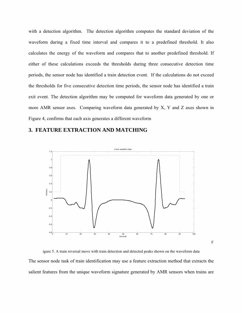
igure 5. A train reversal move with train detection and detected peaks shown on the waveform data

The sensor node task of train identification may use a feature extraction method that extracts the

salient features from the unique waveform signature generated by AMR sensors when trains are

within range of a sensor node. Figure 5 displays Z axis waveform data and sensor node train

detection results for a train that moved within sensor node range, stopped and reversed direction,

moving out of sensor node range in the opposite direction of the initial movement. The AMR

sensor waveform data displayed in Figure 5 shows base reference at 0.03 mGauss between zero

and 5 seconds and between 93 and 95 seconds. The train entered sensor node range at 5 seconds,

continuing to move by the sensor node until about 42 seconds. The essentially flat waveform

between 42 and 50 seconds corresponds to a stopped train. This is confirmed by noting that the

flat waveform is shifted from the base reference of 0.03 mGauss to -0.01 mGauss. At 50 seconds

the train begins to reverse it movement and continues to move in the opposite direction past the

sensor node between 50 and 93 seconds when it moves beyond range of the sensor node. Notice

that the reverse direction waveform (between 50 and 93 seconds) is essentially the mirror image

of the original direction waveform (between 5 and 42 seconds).

Waveform features selected for identification purposes may include the number, magnitude,

sequence of peaks (maxima and minima), and prominent frequency content. Selecting waveform

peaks has the advantage that peaks features remain the same regardless of train speed.

Increasing train speed compresses waveform peaks and decreasing train speed expands

waveform peaks. Peak sequence and important waveform details are preserved with peak

analysis which substantially reduces volume of data that must be processed, transmitted, stored

and compared by the sensor nodes and the VPU, reducing the complexity of the UTIS matching

algorithm. The results of the following peak detection algorithm are indicated in Figure 5 by

small squares ‘□’ placed at the peak locations along the waveform data (z1, z2, z3,………, zn).

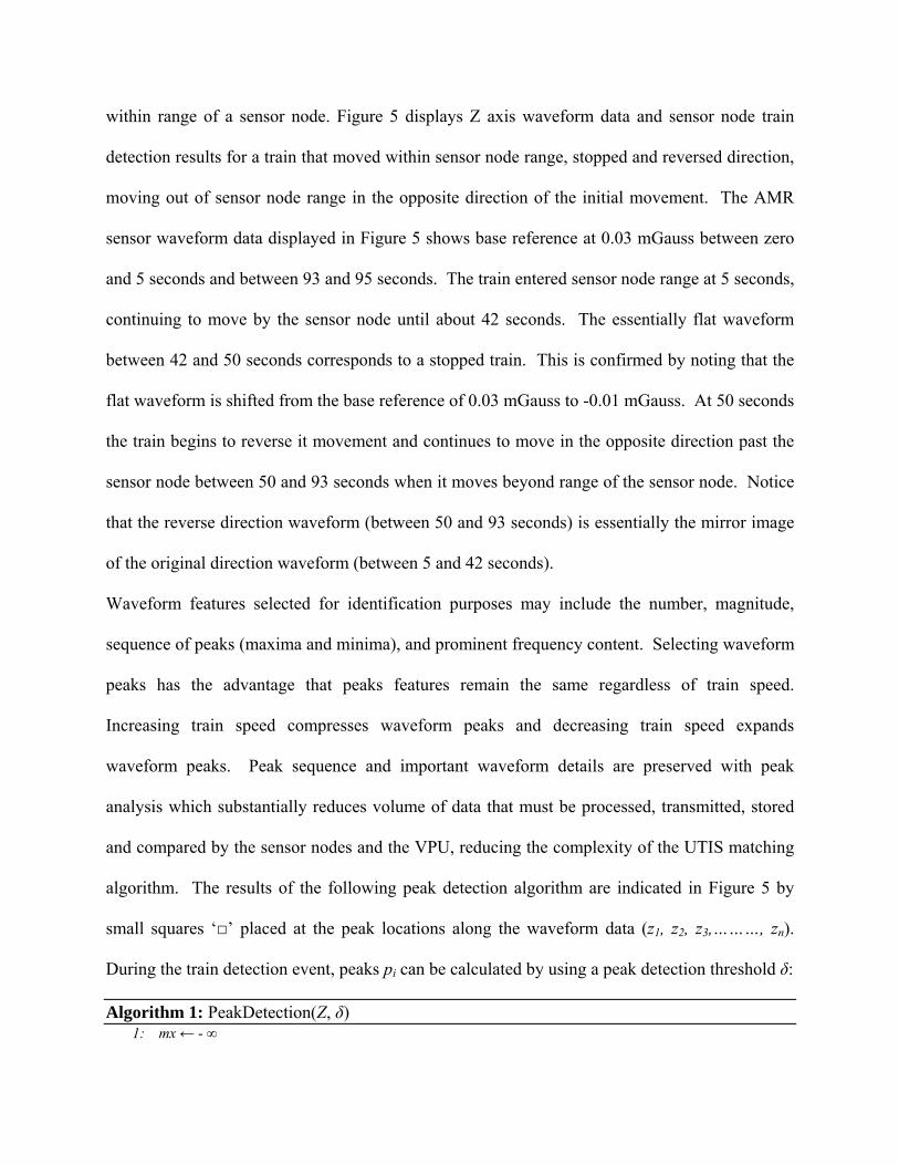
During the train detection event, peaks pi can be calculated by using a peak detection threshold δ:

Algorithm 1: PeakDetection(Z, δ) 1: mx ← - ∞

2: mn ← +∞

3: p[] ← new

4: searchmaxima ← 0

5: for i = 1; i≤ n; i++ do

6: if zi > mx + δ, then

7: mx ← zi

8: end if

9: if zi < mx - δ, then

10: mx ← zi

11: end if

12: if searchmaxima == 1 then

13: if zi < mx - δ, then

14: pi ← zi

15: mn ← zi

16: serachmaxima ← 0

17: end if

18: else

19: if zi > mn + δ, then

20: pi = ← zi,

21: mx = ← zi

22: serachmaxima ← 1

23: end if

24: end if

25: end for

26: return p The series of detected peaks for a given train detection event are given by:

The sequence and time stamped peak values derived from the AMR sensor generated waveform

of a train moving within the train detection zone are calculated and temporarily stored by each

sensor node. Time stamped sequence and peak value data is transmitted by all train detection

zone sensor nodes to the VPU where data from each sensor node is evaluated and compared to

determine if sensor node data matches.

There may be great variability in train movements that occupy the train detection zone. A train

may enter the zone at a certain speed and continue through the entire zone, exiting at the same

speed. A train may enter the zone and increase or decrease speed while transiting the zone. A

train may enter the zone and stop within the zone, eventually resuming the original direction of

movement or reversing its movement within the zone. A train may enter the zone and, with or

without stopping and reverse movements, diverge from the main route, picking up and/or leaving

rail cars and changing the order of cars within the composition of the train, finally resuming or

reversing the original movement into the detection zone. Additional processing is required at the

sensor node to track variations in train movement and composition. In order to provide feature

extraction for a train event without peaks redundancy due to train reversals, it is essential to

detect when a train stops based on the waveform data processing. The following train stop

detection algorithm looks for continuous waveform variation and compares consecutive changes

in waveform to a threshold while also comparing the largest difference in variation to another

predefined threshold. If is the mean value of the waveform data taken over n samples

and is its derivative then following criteria is used to declare vehicle’s motion state by

comparing to thresholds and over M number of derivatives. The thresholds and are

decided empirically from actual train waveform data.

Once the vehicle’s state of motion is identified, further processing will remove peak redundancy.

Figure 5 shows the z-axis waveform data and train detection results of a train that moved within

range of a sensor node, stopped and then reversed out. The train stop detection algorithm will

indicate the stopped train of Figure 5. This indication helps in sub-grouping the peaks that exist

between train stop events or between train stop events and end of detection events. Generally,

the sequence of peaks selected for a train detection event can be represented by:

Where m is the number of stops made by the train in a particular train detection event and ni is

the number of peaks detected in the interval before an ith stop. These sub-groups can be matched

against each other for possible train reversal detection. It is critical to identify train reversal, in

order to remove redundancy in the waveform peaks. Therefore a logic is required that checks for

reverse train movements and tracks direction of movement changes during the train detection

event.

Each subgroup of peaks is matched with its following neighboring subgroup to check for reversal

detection using a Dynamic Time Warping (DTW) method (7). Given two subgroup of peaks,

such that n1=M and n2=N, DTW gives the optimal

solution in the O(MN) time which may be refined further through different techniques such as

multi-scaling (8) (9). If these peaks or sequences are taken from some feature space then for

comparison purposes a local distance measure between can be given by:

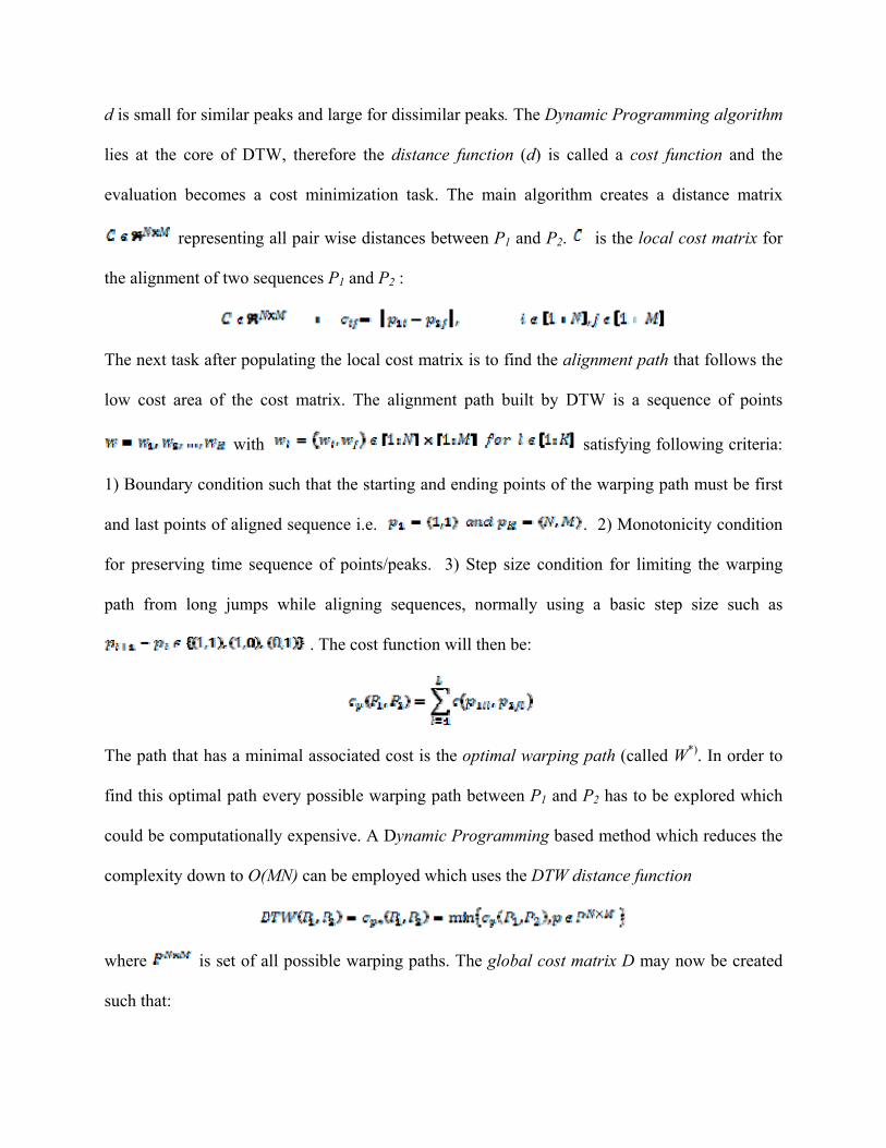
d is small for similar peaks and large for dissimilar peaks. The Dynamic Programming algorithm

lies at the core of DTW, therefore the distance function (d) is called a cost function and the

evaluation becomes a cost minimization task. The main algorithm creates a distance matrix

representing all pair wise distances between P1 and P2. is the local cost matrix for

the alignment of two sequences P1 and P2 :

The next task after populating the local cost matrix is to find the alignment path that follows the

low cost area of the cost matrix. The alignment path built by DTW is a sequence of points

with satisfying following criteria:

1) Boundary condition such that the starting and ending points of the warping path must be first

and last points of aligned sequence i.e. . 2) Monotonicity condition

for preserving time sequence of points/peaks. 3) Step size condition for limiting the warping

path from long jumps while aligning sequences, normally using a basic step size such as

. The cost function will then be:

The path that has a minimal associated cost is the optimal warping path (called W*). In order to

find this optimal path every possible warping path between P1 and P2 has to be explored which

could be computationally expensive. A Dynamic Programming based method which reduces the

complexity down to O(MN) can be employed which uses the DTW distance function

where is set of all possible warping paths. The global cost matrix D may now be created

such that:

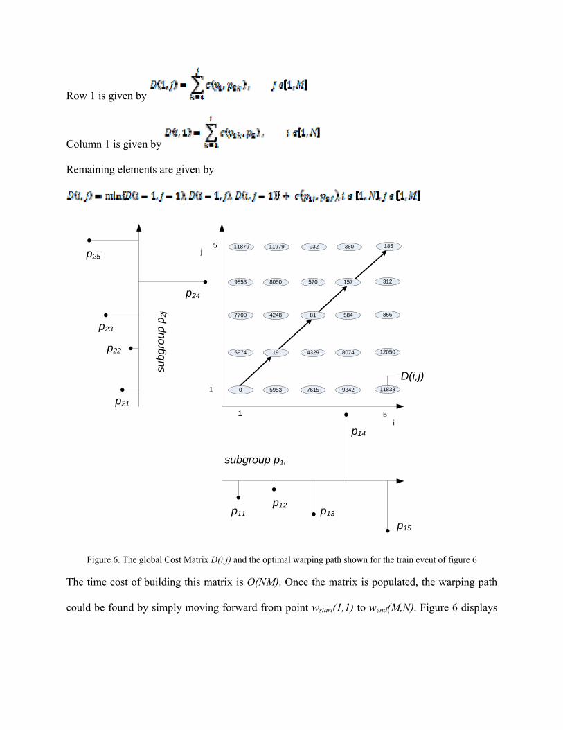
Row 1 is given by

Column 1 is given by

Remaining elements are given by

i

j

1

1

5

5

0 5953 7615 9842 11838

5974 19 4329 8074 12050

7700 4248 81 584 856

9853 8050 570 157 312

11879 11979 932 360 185

p11p12

p13

p14

p15

p21

p22

p23

p24

p25

subgroup p1i

subg

roup

p2

j

D(i,j)

Figure 6. The global Cost Matrix D(i,j) and the optimal warping path shown for the train event of figure 6

The time cost of building this matrix is O(NM). Once the matrix is populated, the warping path

could be found by simply moving forward from point wstart(1,1) to wend(M,N). Figure 6 displays

the Cost Matrix D(i,j) calculated for the waveform data and peaks shown in Figure 5. The

optimal warping path, lowest cost associated, is shown by solid arrows.

The warping path has been established, but the task of matching the two subgroups of peaks

remains. Due to empirical peak detection threshold δ and changing magnetic flux density at a

sensor location, the number and magnitude of peaks detected, even for an exactly same portion

of a train, can be different. Two subgroups of peaks being compared may also differ due to the

number of train cars they represent. For example, one subgroup may represent a partial straight

move of five train cars while the other may represent a partial reverse move of 10 cars.

Therefore, it is essential that the above algorithm be refined to accommodate these variations and

still deliver the best possible match. The method selected examines the subgroups for a sequence

of consecutive low cost matches. If a minimum number of consecutive low cost matches are

found, the following algorithm determines a satisfactory match:

Algorithm 2: FindMatch(P1, P2, w, D, θ1, θ2, θ3) 1: n ← max(|P1|,|P2|)

2: diff ← 0

3: matchfound ← 0

4: LessThanθ1 ← 0

5: LessThanθ2 ← 0

6: LessThanθ3 ← 0

7: for i=1; i ≤ n; i++ do

8: diff ← D(w(i+1,1),w(i+1,2)) - D(w(i,1),w(i,2))

9: if ( diff < θ1 ) then

10: LessThanθ1 ← LessThanθ1 + 1

11: LessThanθ2← 0

12: LessThanθ3 ← 0

13: elseif ( diff < θ2 ) then

14: LessThanθ2 ← LessThanθ2 + 1

15: LessThanθ1 ← 0

16: LessThanθ3 ← 0

17: elseif ( diff < θ3 ) then

18: LessThanθ3 ← LessThanθ3 + 1

19: LessThanθ1← 0

20: LessThanθ2 ← 0

21: end if

22: if (LessThanθ1 == 2) then

23: matchfound ← 1

24: break

25: end if

26: if(LessThanθ2 == 3) then

27: matchfound ← 1

28: break

29: end if

30: if (LessThanθ3 == 4) then

31: matchfound ← 1

32: break

33: end if

34: end for

35: return matchfound

This matching algorithm will identify reversals of train direction. This is accomplished by

matching one subgroup, with a mirror image of the neighboring subgroup of peaks. A match

indicates movement direction has been reversed. The algorithm updates direction of travel every

time movement resumes after a train stop is detected.

Each sensor node transmits a train detection report to the VPU when the train detection event is

complete at that sensor node. This report includes essential features of the AMR waveform

derived by sensor node processing techniques such as peak detection. These techniques remove

redundancies via the sensor node matching algorithm before the train detection report is

transmitted to the VPU. This technique simplifies matching multiple sensor node UTIS

matching at the VPU using the DTW method. These techniques have the flexibility to provide

reliable UTIS matching in spite of variable magnetic fields, train movements and fixed threshold

criteria. If the VPD determines that the UTIS received from all sensor nodes in a train detection

zone match, and all sensor nodes report normal operational status, the VPD output will be

changed from LO to HI, indicating an un-occupied train detection zone.

Data derived from the AMR sensor response to magnetic flux changes caused by locomotives

and rail cars is critical to the vital, fail-safe, closed loop performance of a magnetometer-based

train detection zone. Methods for digitally evaluating and processing the analog data generated

by the AMR sensors are critical to the vitality of the detection zone.

4. CONCLUSION

A vital train detection system utilizing track rail independent magnetometers to establish discrete

train detection zones is feasible. Success requires the use of AMR sensors and dynamic

waveform processing techniques that enable reliable and conclusive matching of unique train

identification signatures derived by multiple sensor nodes reporting to a central vital processing

unit. AMR sensor generated waveform characteristics, appropriate waveform processing, and

robust central processor matching methods are necessary to the vitality and reliability of this

train detection system. This innovative magnetic detection system is compatible with

conventional railroad signal devices and systems. It satisfies vital, fail-safe and closed loop

design principles. It may be deployed as an enhancement of conventional devices or configured

as a stand alone system. It is immune to the effects of rail and ballast contamination, including

salt or other snow-melting/de-icing agents. The sensor nodes and vital processor unit are power

efficient and fully modular. Low power requirements enable the sensor nodes and the vital

processor unit to operate off grid. The system is designed for rapid deployment and remains

easily reconfigurable. Adding or removing sensor nodes from a train detection zone requires

only user programming changes at the central vital processing unit. Possible applications include

stand alone rural crossing train detection systems, auxiliary train detection device for grade

crossing systems installed on poor track or contaminated ballast, auxiliary control system for

railroad crossing highway traffic preemption, and switch protection in classification yards. The

system may be configured to emulate the performance of any track based train detection circuit

from dc track circuit to constant warning devices.

5. ACKNOWLEDGMENTS

The research described herein has been partially funded by USDA SBIR research grants 2007-

33610-18611 and 2006-33610-16783. Railroad test site facilities are provided by Wisconsin &

Southern Railroad, Madison, Wisconsin.

6. REFERENCES [1] 49CFR Part 236.5 Design of Control Circuits on Closed Circuit Principle. Rules,

Standards and Instructions Governing the Installation, Inspection, Maintenance and Repair

of Systems, Devices, and Appliances

[2] Robinson, William, US Patent 130,661, Improvement in Electric-Signaling Apparatus for

Railroads, August 20, 1872.

[3] 49CFR Part 236.56 Shunting Sensitivity. Rules, Standards and Instructions Governing the

Installation, Inspection, Maintenance and Repair of Systems, Devices, and Appliances

[4] Honeywell, Application Note – AN218, Vehicle Detection Using AMR Sensors, August

2005.

[5] Transportation Research Board of the National Academies, High-Speed Rail IDEA Program

Final Report for Project 53, Magnetometer Sensor Feasibility for Railroad and Highway

Equipment Detection, Prepared by Jeff Brawner and K. Tysen Mueller, SENSIS

Corporation, Seagull Technology Center, June 2006.

[6] Eva Signal Corporation, US Patent 7,075427 B1, Traffic Warning System, Joseph R. Pace

and Joseph A. Pace, July 11, 2006.

[7] R. Bellman and R. Kalaba (1959), On adaptive control processes, Automatic Control, IRE

Trans, Vol. 4, No. 2, pp 1-9.

[8] M. Muller, H. Mattes, and F. Kurth (2006), An efficient multiscale approach to audio

synchronization, pp. 192-197.

[9] S. Salvador and P. Chan (2007), Towards accurate dynamic time warping in linear time and

space, Intell. Data Anal., Vol. 11, No. 5, pp. 561-580.

7. LIST OF FIGURES AND ALGORITHMS Figure 1. DC Track Circuit Diagram

Figure 2. Magnetic Train Detection Zone Diagram

Figure 3. Magnetic Train Detection Zone with Track Switch Diagram

Figure 4. Three dimensional AMR sensor waveform data of a train and detection results

Figure 5. A train reversal move with train detection and detected peaks shown on the

waveform data

Figure 6. The global Cost Matrix D(i,j) and the optimal warping path shown for the train

event of Figure 6

Algorithm 1: PeakDetection(Z, δ) Algorithm 2: FindMatch(P1, P2, w, D, θ1, θ2, θ3)