An integrated Bayesian model for DIF analysis

Tufi M. Soaresa, Flavio B. Goncalvesa and Dani Gamermanb

a Centro de Polıticas Publicas e Avaliacao da Educacao, Departamento de Estatıstica, Universidade Federal de Juiz de Fora.b Departamento de Metodos Estatısticos, Instituto de Matematica, Universidade Federal do Rio de Janeiro.

Abstract

In this paper, an integrated Bayesian model for DIF (Differential Item Functioning) analysisis proposed. Integrated in the sense of modelling the responses along with the DIF, thus allowingDIF detection and DIF explanation in a simultaneous setup. Previous empirical studies and/orsubjective beliefs about the items parameters, including differential functioning behavior, may beconveniently expressed in terms of priors distributions and imposed to the model. In this context,it is not necessary, as usual, to specify a set of items without DIF to get a correct identification ofthe model. It is enough to choose appropriate informative prior distributions for a small number ofitens. It reduces the iterative procedures that are commonly used for proficiency purification andDIF detection and explanation. Examples demonstrate the efficiency of this method in simulatedand real situations.

Key Words: Bayesian analysis, Item Response Theory, Differential Item Functioning.

1

XXXIX SBPO [386]

1 Introduction

The Differential Item Functioning (DIF) analysis has been very important in educational researchsince the 1960’s. Its importance is shown in a large number of applied studies. For instance, studieson performance differences in items of educational assessment tests (like GRE, SAT, GMAT, etc.)in groups defined by different ethnic characteristics, gender and socioeconomic status have been fre-quently shown in literature (eg. O’Neil & McPeck (1993), Shimitt & Bleinstein (1987), Berberoglu(1995), Gierl et al. (2003) and cited references). Therefore, it is not surprising that several statisticalmethods have been developed in order to support empirical analysis. The profusion of methods forthe detection of items with DIF stands out. Some of the most used ones are: Mantel-Haenszel statisticbased procedures (particularly the MH D-DIF statistic, cf. Dorans & Holland (1993)), the logistic re-gression method (Swaminathan & Rogers, 1990), the Simultaneous Item Bias Test - SIBTEST (Shealy& Stout, 1993) and methods that use the item parameters from Item Response Theory (IRT) models(Lord, 1980; Thissen, Steinberg & Wainer, 1993). Other methods are found, for example, in Clauser& Mazor (1998).

The first three methods cited above depend, directly or indirectly, from a previous estimation ofthe ability or from alternative criteria for the individuals equalization, which, in general, can not bedissociated from the DIF existence. Therefore, the ability purification in successive stages is recom-mended where the DIF item detected (in each stage) are eliminated from the ability calculation for thenext analysis (Holland & Thayer, 1988; Wang & Su, 2004). On the other hand, the methods basedon IRT models construction, like IRT-LR and IRT-D2 (Thissen, Steinberg & Wainer, 1993), postulatethat a subset of anchor items, for which the non existence of DIF is assumed, is defined a priori andit is proposed to compare two models in successive stages by using likelihood ratio tests. The an-chor items can remain constant or vary in different stages depending on the results of the tests (Wang& Yeh, 2003). In any case, all these proposals involve different stages of DIF parameters detectionand decision about which items have DIF. May (2006) proposes an extension of the standard gradedresponse model (Samejima, 1997) which allows the overall threshold (difficulty) and discriminationparameter to vary across different groups, except for a set of anchor itens.

The detection of items with DIF is an important step in DIF analysis, but a complete analysis alsorequires some other important steps like a satisfactory classification of the DIF found, the identifica-tion of the factors associated to DIF along with the respective hypotheses formulation related to theDIF causes and maybe, a hypotheses confirmatory analysis. For example, Schmitt, Holland & Dorans(1993) suggest that specially planned studies should be used to confirm the hypotheses formulatedfrom the DIF factors study. In this context, it is natural to construct regression models that associateco-variables, related to the items, to the DIF’s magnitude. The co-variables would represent the DIFfactors in such a way that the regression analysis’ results would confirm or not the formulated hy-potheses. Longford, Holland & Thayer (1993) proposed a random effects regression model where theparameters of the model vary according to different forms of the test ministration and, in addition, theDIF’s magnitude is explained by variables correlated to the items (in particular, a difficulty measureof the item). Rogers & Swaminathan (2000) used characteristics of the individuals on the second levelof their two level model to improve the equalization between the members of the reference and focalgroups. Swanson et al. (2002) propose an extension of the logistic regression method of Swami-nathan & Rogers (1990) imposing an hierarchical structure where characteristics related to the itemsvia co-variables are included on the second level of the regression model allowing the confirmation orrejection of the hypotheses about DIF.

Once again, all the three approaches above require the previous determination of the ability or ofa DIF measure. In addition, the detection and the explanation (through associated factors) steps are

2

XXXIX SBPO [387]

taken separately.The importance of Bayesian approaches has been steadily growing in Item Response Theory. For

example, Bayesian estimation methods are used in IRT models in several approaches (e.g. Albert(1992), Patz & Junker (1999a), Patz & Junker (1999b), Fox & Glas (2001), Beguin & Glas (2001)).Particulary, DIF analysis is an appropriate environment for a genuine Bayesian formulation due to thecomplex structure of the models and the subjective decision features involved, which can be formu-lated through Bayesian arguments. For example, Zwick, Thayer & Lewis (1999, 2000) and Zwick &Thayer (2002) consider a formulation where the MH D-DIF statistic is represented by a normal modelwhere the mean is equal to the “real DIF parameter” for which a normal prior distribution is explicitlyconsidered. These authors use Empirical Bayes (EB) for the posterior estimation of the parameters.Sinharay et al. (2006) consider the same formulation and propose informative prior distributions basedon past information and show that the “Full Bayes” (FB) method leads to improvements if comparedto the two other approaches, specially in small samples.

This paper presents an integrated Bayesian approach for DIF detection and analysis, which reducesor even eliminates the need of analysis with many steps. In the proposed model, the anchor items (andthe items with DIF) are identified simultaneously along with the estimation of all the other parametersof the model. Also, a regression structure associated to the DIF parameters is introduced in sucha way that DIF explanation can be analyzed along with the ability simultaneously. Naturally, themodel presents the conditions to be used in a confirmatory and explanatory analysis. An examplewith simulated data are presented considering 2 groups. An analysis with real data concerning aneducational program in the state of Rio de Janeiro, Brazil, is also presented.

2 Model for DIF Analysis

Typically, in educational assessment, a test is formed by I items, but student j only answers a subsetI(j) of these items. Let Yij , j = 1, . . . , J , be the score attributed to the answer given by the studentj to the item i ∈ I(j) ⊂ {1, . . . , I}. Only the dichotomic case, where one of the scores in {0, 1} isattributed to the item will be considered. This way, Yij = 1 if the answer is correct and Yij = 0 ifthe answer is wrong. In general, there can be different types of DIF (see Hanson (1998) for a widercharacterization), but restricted to the characteristics which are made explicit by the three parametersmodel - 3PL (Birnbaum, 1968), the types of DIF can be immediately characterized according to thedifficulty, discrimination and guessing. This paper will not consider the possibility of DIF in theguessing parameter. Although it is possible, the applicability of this case considering the conventional3PL model is substantially limited by the known difficulties in the estimation of this parameter and bypractical restrictions.

Define P (Yij = 1|θj , ai, bi) = pij , and consider logit(pij) = ln(

pij

1− pij

). If logit(pij) = ∆ij ,

then pij = logit−1(∆ij) =1

1 + e−∆ij. The main structure of the model used in this paper to associate

the student’s answer to his/her ability is:

P(Yij = 1|θj , ai, bi, ci, d

aig(j), d

big(j)

)= ci + (1− ci)logit−1(∆ij) (1)

where ∆ij = Deda

ig(j)ai(θj − bi + dbig(j))

for i = 1, . . . , I , j = 1, . . . , J and g = 1, . . . , G, g(j) is the group the student j belongs to.Let aig = eda

igai (> 0) be the item’s discrimination parameter, big = bi − dbig be the item’s

difficulty parameter and ci (∈ [0, 1]) be the item’s guessing parameter. Suppose that the students are3

XXXIX SBPO [388]

grouped in G known groups and, a priori, θj |λg(j) ∼ N(µg(j), σ2g(j)), where λg(j) = (µg(j), σ

2g(j)). It

is assumed that λ1 = (µ1 , σ21) = (0, 1) to guarantee the identification of the model. On the other hand,

λg = (µg, σ2g), g = 2, . . . , G, is unknown and must be estimated along with the other parameters.

Besides that, dbig (db

i1 = 0) represents the DIF related to the difficulty of the item in each group andeda

ig (dai1 = 0) represents the DIF related to the discrimination of the item in each group.

It is possible to use covariates to explain the DIF parameters dhig, i = 1, . . . , I, g = 2, . . . , G, h =

a, b. It is assumed the following structure for these parameters:

dhig ∼

(1− πh

ig

)N(0, s2

i (τhg )2)

+ πhigN

(W h

i γhg , (τh

g )2)

(2)

The Normal distribution in (2) defines the regression model where W h is the design matrix, γhg is

the vector of coefficients and(τhg

)2is the item’s specific random factor in group g for parameter h.

This kind of mixture is used by George & McCulloch (1993) to propose a Bayesian model for variableselection in a regression model.

The distribution in (2) can be written as follows:

dhig ∼ N

((W h

i γhg

)Zh

ig , [s2i ]

1−Zhig(τh

g )2)

. (3)

3 Bayesian Inference

Define Ψ = {Ψ1,Ψ2,Ψ3}, where Ψ1 = {θ, λ}, Ψ2 = {a, b, c} e Ψ3 = {d, π, γ, τ}, and eachcomponent represents the correspondent parameter with all possible indexes, for example: θ ={θ1, . . . , θJ}. The main aim of the inference process is to obtain the joint posterior p(Ψ|Y, W ) distri-bution given by:

p(Ψ|Y, W ) =p(Y |Ψ)p(Ψ|W )∫

. . .∫

p(Y |Ψ)p(Ψ|W )dΨ(4)

Since it is very hard to obtain the explicit expression for the distribution above, MCMC (MarkovChain Monte Carlo) methods are used to draw a sample of this distribution and approximate it (seeGamerman & Lopes (2006) for details). It is possible to have problems when using MCMC algo-rithms: they may converge to local modes that do not estimate the parameters efficiently. The choiceof the initial values of the chains has a great influence on the local modes convergence problem. Sim-ulated examples presented in Goncalves (2006) show that it is crucial to set the initial values of theparameters dh

ig as zero to obtain good estimates of the model’s parameters. Different initial values leadto convergence to local modes.

It is assumed, a priori, that Ψ1, Ψ2 and Ψ3 are independent, that is: p(Ψ) =3∏

i=1

p(Ψi). The

following prior distributions are used for the Ψ′is:

P (Ψ1) =J∏

j=1

p(θj |µg(j), σ2g(j))

G∏g=2

p(µg)p(σ2g)

where: (θj |µg(j), σ2g(j)) ∼ N(µg(j), σ

2g(j)) , µg ∼ N

(m0, s

20

)and σ2

g ∼ IG (α0, β0),∀j = 1, . . . , J and ∀g = 2, . . . , G, where IG is the Inverse Gama distribution.

4

XXXIX SBPO [389]

p(Ψ2) =I∏

i=1

p(ai)p(bi)p(ci)

where: ai ∼ LN(mai , s

2ai

); bi ∼ N

(mbi

, s2bi

)and ci ∼ beta (αci , βci) , ∀i = 1, . . . , I ,

where LN is the Log-Normal distribution, and defining γhg = γ0g, γ1g, . . . , γKhg and W = W a,W b,

the prior distribution of Ψ3 is:

p(Ψ3|W ) =∏

h=a,b

G∏g=2

(I∏

i=1

p(dh

ig|πhig,W

h, γhg , (τh

g )2)

p(πhig)

)p(γh

g )p((τh

g )2)

where:(dh

ig|πhig,W

h, γhg , (τh

g )2)∼ N

((W h

i γhg

)πh

ig , [s2i ]

1−πhig(τh

g )2)

. πhig ∼ Ber

(ξhig

). γh

g ∼

NKh+1

(mγh

g, s2

γhgIKh+1

)and (τh

g )2 ∼ GI(ατhg, βτh

g), for h = a, b , ∀i = 1, . . . , I and ∀g =

2, . . . , G.The decision on the classification of an item as having or not DIF is based on the parameters πh

ig.A simple classification rule decides based on the posterior mean of πh

ig. If it is greater than a p∗, item iis classified as having DIF in parameter h, in group g regarding group 1 and vice-versa if it is smallerthan p∗. Carefully attention must be paid to items of which πh

ig is very close to p∗. In this paper it isassumed p∗ = 0.5, but more elaborated criteria may be used to choose the value of p∗, for example,based on other loss functions (see Migon & Gamerman (1999)). Once the item is classified, it is onlynecessary to analyse the DIF parameters of the items classified as DIF ones, for the other items, theDIF parameter is assumed to be 0.

An important issue concerning DIF analysis is how to proceed in a situation with more than 2groups. Since the detected and estimated DIF in group g refers to group 1 (reference group), theanalysis must be done the following way: if a certain item is detected as a non DIF one in N groups,then, there’s no DIF between these N groups, since the item behaves the same way in these groups.If a certain item is detected as a DIF one in a group and as a non DIF one in another group, then,the interpretation is the same as between the group where the item has DIF and the reference group.Finally, if an item has DIF in two groups, the estimatives of the DIF parameters of this item in bothgroups must be compared since they have the same scale.

4 Simulated example

In the example of this section, the parameters of the items and the abilities are randomly drawn. Theabilities are drawn from a standard normal distribution for the reference group and from a N(−0.25, (1.2)2)distribution for the focal group (and G = 2). The discrimination parameters ai are drawn from aLN(0.2, 0.3) distribution, the difficulty parameters bi are drawn from a standard normal distributionand the guessing parameters ci from a beta distribution with parameters (41, 161).

The items with DIF are also randomly chosen. In this example, 28 items (70% of all the items) arechosen to have DIF, and then, 12 items are chosen not to have DIF. 27 items have DIF in the difficultyparameter, 9 in the discrimination parameter and 8 of these items have DIF in both parameters. Theparameter db

i2, which represents the DIF in the difficulty parameter of the item i, is drawn from aN(W b

i γb2 , (τ b

g )2)

distribution, ∀i = 1, . . . , I , where (τ bg ) = 0.2. Also γb

2 = (0.20, 0.40)T andW b

i = (1,W bi2) where W b

i2 = 1 for 9 randomly chosen for 9 items with DIF and W bi2 = 0 for the

other items, simulating the effect of a binary covariate associated to a common characteristic of these5

XXXIX SBPO [390]

9 items. The parameter dai2, which represents the DIF in the discrimination parameter of the item i, is

drawn from a N(W a

i γa2 , (τa

g )2)

distribution, ∀i = 1, . . . , I , where (τ bg ) = 0.2 and γa

02 = −0.30. Nocovariate was used for the DIF parameters in the discrimination.

From the drawn parameters of the items and of the abilities, the answers of 4000 students weredrawn for a set of 40 dichotomic items. The students were separated in two groups of 2000 studentseach.

The convergences of the Markov chains drawn from the Gibbs Sampler were tested using the Rcriteria of Gelman & Rubin (RGR) (see Gamerman & Lopes (2006) for details), calculated from 4parallel chains after 10,000 iterations and different initial values. The test showed that all the chainsconverged with RGR < 1.1 for all of them.

It was chosen s2i = (400000)−1 for DIF in difficulty and s2

i = (100000)−1 for DIF in discrim-ination. The results for this study are shown in table 1 and figures 1 and 2. An item is identified ashaving DIF if the posterior mean of its respective πh

ig is greater than 0.5. As observed in figure 1, themethod of DIF identification had a very acceptable performance. With regards to the difficulty, only 6out of 40 items were misidentified (items 6, 9, 10, 16, 29 and 35). However, the real value of the DIFparameters of the items 6 and 9 are very small (0.0211 and -0.0483 respectively), making it reasonableto identify these items as not having DIF. In the other misidentified cases, the estimates of the DIFparameters vary between 0.0789 and 0.1293 in absolute values, which can be considered small DIF’s.Anyway, the misidentification had a very little effect in the BIAS statistics. Similar conclusions canbe made about the discrimination parameters.

Figure 1: Posterior mean of parameters πhig in difficulty (left) and discrimination (right) and classifi-

cation of the items. The points and triangles represent the actual status of the items, with DIF (points)or without DIF (triangles).

Parameter Real value Estimated value Credibility intervalµ1 0.0042 0 (0 , 0)µ2 -0.2961 -0.3400 (-0.4174 , -0.2617)σ1 0.9758 1 (1 , 1)σ2 1.1861 1.1838 (1.1043 , 1.2823)γa02 -0.3 -0.2301 (-0.5905 , -0.0592)

τa2 0.3 0.4226 (0.2002 , 0.8148)

γb02 0.2 0.1998 (0.0774 , 0.3326)

γb12 0.4 0.2511 (0.0483 , 0.4562)τb2 0.2 0.2131 (0.1597 , 0.2821)

Table 1: Estimation of the parameters of the abilities’ distribution and of the parameters of the DIFregression.

6

XXXIX SBPO [391]

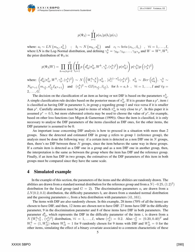
Figure 2: Comparison of the real and the estimated item parameters (with credibility intervals).The points represent the real value of the parameters, the vertical lines represent the posterior 95%credibility intervals and the horizontal lines inside the intervals represent the posterior mean. Toprow: the difficulty parameter for the reference group (left) and for the focal group (right); middle row:the discrimination parameter for the reference group (left) and for the focal group (right); bottom row- guessing parameter.

5 Application

The real data set analysed in this paper refers to an education program called Nova Escola. Thisprogram was created by the Rio de Janeiro State Government in the year 2000 and propose criteria toevaluate all the 1854 schools of the State education net. The evaluated grades are from 2nd to 8th inelementary school and from 1st to 3rd of high school in two disciplines, Portuguese and Mathematics.The main objective of the program is to improve the teaching quality and prize public schools. Thereal data set analysed in this paper refers to the Maths test applied to the 5th grade in the year 2005.67283 students were evaluated, from which 3998 are from the State Capital (Rio de Janeiro city).Due to computational price, a sample of 7998 students is randomly sampled to be analysed: all the3998 from the Capital and 4000 from the other cities. This is the group division chosen for the DIFanalysis. The 56 items are separated into 7 blocks of 8 items and the tests are formed by 3 blocks viaincomplete balanced blocks. Each student answers to one of these tests. The tests are composed ofmultiple choice items with 4 options each, where only one is correct.

The items analysis is based on the Mantel-Haenszel statistic for the difficulty and in the subjectiveanalysis of the items empirical curve for the discrimination. The group of the students from theCapital is defined as the reference group in the DIF analysis. Differential functioning was observed in

7

XXXIX SBPO [392]

the items shown in table 2.

DIF ItensDiscrimination 2, 9, 13, 14, 16, 20, 34, 37, 38, 39

Difficulty 13, 16, 17, 20, 22, 32, 33, 37, 38, 41, 44, 46, 52, 53

Table 2: Items for which DIF was detected.

From the items with significant positive DIF in the difficulty (more difficult for the students fromthe Capital), four of them (17, 32, 44 and 52) are related to the interpretation of bar plots. The items 42and 54 are also related to this content, but their AlfaD Mantel-Haenszel statistics are small (0.63 and0.25, respectively). Significant DIF was considered for items with absolute value of the AlfaD Mantel-Haenszel statistics greater than 0.90. From the items with significant negative DIF (13, 20, 37, 46, 53)in the difficulty, all of them are related to the calculation of changes. On the other hand, the items 5,19 and 34 are also related to this content but have small AlfaD Mantel-Haenszel statistics (-0.46, -0.22and -0.14, respectively). These are very interesting results and possibly very important in the BrazilianMathematics Education community. Based on these results, the analysis will be performed includingindicator variables related to the items contents cited above. Based on the opinion of specialists and onthe results of the preliminary analysis, the chosen values for the prior probability of an item presentingDIF were: 0.90 for the items for which DIF was detected and 0.1 for the other ones, according to thedifficulty; for the discrimination, these values were 0.7 and 0.3 respectively. Therefore, no item wasfixed as an anchor one. The choice of these probability values was based on the expected numberof answers in the sample for each item (around 1700) and considering that it is desired that the priordistribution has an important influence on the posterior distribution.

The results of this analysis are presented in table 3, and figures 3 and 4.

Parameter Estimated value Credibility intervalµ2 -0.175 (-0.217 , -0.129)σ2 0.822 (0.787 , 0.858)γa02 0.081 (-0.468 , 0.556)

(τa2 )2 0.384 (0.069 , 1.420)

γb02 0.228 (0.043 , 0.423)

γb12 0.015 (-0.260 , 0.286)

γb22 -0.469 (-0.724 , -0.219)

(τb2 )2 0.055 (0.030 , 0.102)

Table 3: Estimation of the parameters of the abilities’ distribution and of the parameters of the DIFregression.

Item 38 presents a high value (7.48) for the difficulty parameter and a very small value for dis-crimination parameter (0.18), (the difficulty parameter of item 38 is not presented in its correspondentgraph due to its high value). Besides that, it presents a small value for the bisserial correlation (0.05).In original classical IRT analysis using Bilog-mg, item 38 was eliminated because it is a very difficultitem but the item was kept in the analysis presented here. The DIF identification for this kind of itemmust be carefully analysed, because it can be due to the difficulties in the estimation of the parametersof the model.

The results presented in figures 3 and 4 show that only the items 16, 38 and 39 were identified ashaving expressive DIF in the discrimination with posterior probability greater than 0.5. Concerningthe difficulty, the number of items with posteriori probability greater than 0.5 is much larger, precisely24. Among them are all the items related to the two covariates, all the other ones identified in thepreliminary analysis and five other ones not detected. So, the model was very sensitive in the identifi-

8

XXXIX SBPO [393]

Figure 3: Estimation results with credibility intervals for the application. The vertical lines representthe posterior 95% credibility intervals and the dots inside the intervals represent the posterior means.Top row: the difficulty parameter for the reference group (left) and for the focal group (right); middlerow: the discrimination parameter for the reference group (left) and for the focal group (right); bottomrow - guessing parameter.

Figure 4: Posterior probabilities of having DIF in difficulty (left) and discrimination (right) andclassification of the items.

cation of items with DIF, probably because of the combination of the parameters s2ib = 1/400000 and

s2ia = 1/200000, and because of the prior distributions used.

Based on the results of the regression shown in table 3, there is substantial evidence that the itemsrelated to change are easier for the students from the Capital as the posterior mean of γb

22 is −0.469with credibility interval (-0.724 , -0.219). On the other hand, the other covariate does not seem to besignificant, since its posterior mean coefficient is 0.015 with credibility interval (-0.2600 , 0.2867).

9

XXXIX SBPO [394]

6 Conclusions

In this paper, an integrated Bayesian model for detection of items with differential functioning andexplanation of the differential functioning by regression structures with covariates associated to theitems was presented and studied. The model can be used as it is commonly done in literature: bymaking a previous choice of a subset of anchor items. But it can also be used when one is not sureabout an item having or not DIF. In this case, the viability of using a more general model was shown,getting around the difficulties associated with the existence of multi-mode posterior distributions, bychoosing appropriate initial values for the chains.

A simulated study showed a good recovery of the generated parameters and a real example showedthe viability of using the model in practical situations with satisfactory and intuitively consistent re-sults. Nevertheless, improvements in the model can still be needed. Examples are incorporation ofcorrelation structures between the DIF magnitude and the item’s difficulty, and among the DIF in thedifferent items. These are possible directions for future works. On the other hand, the method forDIF detection proposed in this paper presents difficulties when there is no or little knowledge a prioriabout the items having or not DIF. Other possibilities can be sought.

More structured methods for DIF detection can be proposed and compared to the one presentedhere. Other models are already being studied by the authors of this paper and will be reported in futurework.

References

Albert, J. H. (1992). Bayesian estimation of normal ogive item responses curves using Gibbssampling. Journal of Educational Statistics, 17, 251-269.

Beguin, A. A. & Glas, C. A. W. (2001). MCMC estimation and some model-fit analysis of multi-dimensional IRT models. Psychometrika, 66, 541-562.

Berberoglu, G. (1995). Differential item functioning (DIF) analysis of computation, word problemand geometry questions across gender and SES groups. Studies in Educational Evaluation, 21, 439-456.

Birnbaum, S. (1968). Some latent traits models and their use in inferring an examinee’s ability.In Lord, F. & Novick, M. (Eds.), Statistical Theories of Mental Test Scores, 397-472. Reading, MA:Addison Wesley.

Clauser, B. E. & Mazor, K. M. (1998). Using statistical procedures to identify differential itemfunctioning test items. Educational Measurement: Issues and Practice, 17, 31-44.

Dorans, N. J. & Holland, P. W. (1993). DIF detection and description: Mantel-Haenszel andstandardization. In P.W. Holland & H. Wainer (Eds.), Differential item functioning, 35-66. Hillsdale,NJ: Lawrence Erlbaum Associates.

Fox, J. P. & Glas, C. A. W. (2001). Bayesian estimation of a multilevel IRT model using Gibbssampling. Psychometrika, 66, 271-288.

Gamerman, D. & Lopes, H. L. (2006). Markov Chain Monte Carlo: Stochastic simulation forBayesian inference (2rd ed.). New York: Taylor & Francis.

George, E. I. & McCulloch, R. E. (1993). Variable selection via Gibbs sampling. Journal ofAmerican Statistical Association, 85, 398-409.

Gierl, M. J., Bisanz, J., Bisanz, G. & Boughton, K. (2003). Identifying content and cognitive skillsthat produce gender differences in mathematics: A demonstration of the DIF analysis framework.Journal of Educational Measurement, 40, 281-306.

10

XXXIX SBPO [395]

Goncalves, F. B. (2006). Bayesian Analysis of the Item Response Theory: a Generalized Ap-proach. Unpublished M.Sc. dissertation, IM-UFRJ (in Portuguese).

Hanson, B. A. (1998). Uniform DIF and DIF defined by Differences in Item Response Functions.Journal of Educational and Behavioral Education, 23, 244-253.

Holland, P. W. & Thayer, D. T. (1988). Differential item performance and the Mantel-Haenszelprocedure. In H. Wainer & H. Braun (Eds.), Test Validity, 129-145. Hillsdale, NJ: Lawrence ErlbaumAssociates.

Longford, N. T., Holland P. W. & Thayer, D. T. (1993). Stability of the MH D-DIF statistics acrosspopulations. In P.W. Holland & H. Wainer (Eds.), Differential item functioning, 171-196. Hillsdale,NJ: Lawrence Erlbaum Associates.

Lord, F.M (1980). Applications of item response theory to practical testing problems. Hillsdale,NJ: Lawrence Erlbaum Associates.

May, H. (2006). A multilevel Bayesian item response theory method for scaling socioeconomicstatus in international studies of education. Journal of Educational Behavioral Statistics, 31, 63-79.

Migon, H. S. & Gamerman, D. (1999). Statistical Inference: An integrated Approach. Arnold,London.

O’Neil, K. A. & McPeek, W. M. (1993). Item and test characteristics that are associated withdifferential item functioning. In P.W. Holland & H. Wainer (Eds.), Differential item functioning, 255-276. Hillsdale, NJ: Lawrence Erlbaum Associates.

Patz, R. J. & Junker, B. W. (1999a). A straightforward approach to Markov chain Monte Carlomethods for item response models. Journal of Educational and Behavioral Statistics, 24, 146-178.

Patz, R. J. & Junker, B. W. (1999b). Applications and Extensions of MCMC in IRT. Journal ofEducational and Behavioral Statistics, 24, 342-366.

Rogers, H. J. & Swaminathan, H. (2000). Identification of factors that contribute to DIF: Ahierarchical modeling approach. Paper presented at the Annual Meeting of the National Council onMeasurement in Education, New Orleans, LA.

Samejima, F. (1997). Graded response model. In W. J. van der Linden & R. K. Hambleton (Eds.),Handbook of modern item response theory, 85-100. New Yorg: Springer Verlag.

Schmitt, A. P. & Bleistein, C. A. (1987). Factors affecting differential item functioning for blackexaminees on scholastic aptitude test analogy items (ETS RR-87-23). Princeton, NJ: EducationalTesting Service.

Schmitt, A. P., Holland, P. W. & Dorans, N. J. (1993). Evaluating hypotheses about differen-tial item functioning. In P.W. Holland & H. Wainer (Eds.), Differential item functioning, 281-316.Hillsdale, NJ: Lawrence Erlbaum Associates.

Shealy, R. T. & Stout, W. F. (1993). An item response theory model for test bias and differen-tial test functioning. In P.W. Holland & H. Wainer (Eds.), Differential item functioning, 197-239.Hillsdale, NJ: Lawrence Erlbaum Associates.

Sinharay, S., Dorans, N. J., Grant, M. C., Blew, E. O. & Knorr, C. M. (2006). Using past datato enhance small-sample DIF estimation: A Bayesian approach. Technical report, ETS RR-06-09.Princeton, NJ: Educational Testing Service.

Swaminathan, H. & Rogers, H. J. (1990). Detecting differential item functioning using logisticregression procedures. Journal of Educational Measurement, 27, 361-370.

Swanson, D. B., Clauser, B. E., Case, S. M., Nungester, R. J. & Featherman, C. (2002). Anal-ysis of differential item functioning (DIF) using hierarchical logistic regression models. Journal ofEducational and Behavioral Statistics, 27, 53-75.

Thissen, D., Steinberg, L. & Wainer H. (1993). Detection of differential item functioning us-

11

XXXIX SBPO [396]

ing the parameters of item response models. In P.W. Holland & H. Wainer (Eds.), Differential itemfunctioning, 67-114. Hillsdale, NJ: Lawrence Erlbaum Associates.

Wang, W.-C. & Yeh, Y-L. (2003). Effects of anchor item methods on differential item functioningdetection with the likelihood ratio test. Applied Psychological Measurement, 27, 1-20.

Wang, W.-C. & Su Y.-H. (2004). Effects of average signed area between two item characteristicscurves and test purification procedures on the DIF detection via the Mantel-Haenszel method. AppliedMeasurement in Education, 17, 113-144.

Zwick, R., Thayer, D. T & Lewis, C. (1999). An empirical Bayes approach to Mantel-HaenszelDIF analysis. Journal of Educational Measurement, 36, 1-28.

Zwick, R., Thayer, D. T & Lewis, C. (2000). Using loss functions for DIF detection: An empiricalBayes approach. Journal of Educational and Behavioral Statistics, 25, 225-247.

Zwick, R. & Thayer, D. T. (2002). Application of an empirical Bayes enhancement of Mantel-Haenszel DIF analysis to a computerized adaptive test. Applied Psychological Measurement, 26,57-76.

12

XXXIX SBPO [397]