an integrated drainage network analysis system for ...directory.umm.ac.id/data...

An integrated drainage network analysis system

for agricultural drainage management.

Part 2: the application

Xihua Yanga,*, Qiming Zhoub,1, Mike Melvillec,2

aSchool of Information Technology, Charles Sturt University, Bathurst, NSW 2795, AustraliabDepartment of Geography, Hong Kong Baptist University, Kowloon Tong, Kowloon, Hong Kong

cSchool of Geography, University of New South Wales, Sydney 2052, Australia

Accepted 12 July 1999

Abstract

This is the second of two papers that elaborate on an integrated drainage network analysis system

(IDNAS) for agricultural drainage management. In the ®rst paper, the system components,

functions and implementation were presented. This paper focuses on the system applications to

agricultural drainage management, particularly on the acid drainage problems in an estuarine acid

sulfate soil ¯oodplain environment. Four case studies are presented which address practical

drainage management tasks in an acidic sugarcane area in northern New South Wales, Australia.

These tasks are: (1) determine the isochrones (contour lines of equal time of ¯ow) to the watershed

outlet and the drainage areas that contribute to the isochrones; (2) assess the capacity of the existing

drainage network; (3) estimate the accumulated acidic pollutant (total pollutant load) at an outlet

within given times; and (4) simulate acid out¯ow events and predict the amount of acidic pollutant

discharged to the river system associated with each event. The results of these case studies can be

used for ef®cient assessment of acid control practice and for development of better management

policies. It is demonstrated that the IDNAS can be used effectively to simulate the water balance

and drainage network over an agricultural watershed, and to aid the drainage management in an

estuary ¯oodplain environment. # 2000 Elsevier Science B.V. All rights reserved.

Keywords: Agricultural drainage; Acid sulfate soils; GIS; Management

Agricultural Water Management 45 (2000) 87±100

* Corresponding author. Tel.: �612-63384780; fax: �612-63384649.

E-mail addresses: [email protected] (X. Yang), [email protected] (Q. Zhou),

[email protected] (M. Melville)1 Tel.: 852-23395048; fax: 852-23395990.2 Tel.: 612-93854391; fax: 612-93137878.

0378-3774/00/$ ± see front matter # 2000 Elsevier Science B.V. All rights reserved.

PII: S 0 3 7 8 - 3 7 7 4 ( 9 9 ) 0 0 0 6 8 - 2

1. Introduction

In recent years, massive fish kills and fish diseases have been reported in some

Australian estuaries (e.g. Easton, 1989; Tunks, 1993; Callinan et al., 1993). It is now clear

that such phenomena are related to the contamination of estuaries by toxic drainage water

from acidic soils found in Australian coastal floodplains (Willett et al., 1993). These soils

have been recently recognized as a distinct soil group termed as acid sulfate soils (ASS)

which exist along most of the Australian coastline and in other coastal areas around the

world. These soils are very acidic (pH < 3.5) and contained more iron pyrite (FeS2),

which when oxidized, formed more sulfuric acid than was able to be neutralized by the

soil buffering capacity (Melville et al., 1993). The problems associated with acid sulfate

soils have also begun to be recognized as the causes of a great number of environmental

problems, such as changes in ecosystem and aquatic communities, poor agricultural

production, and also corrosion of infrastructure made of concrete or steel.

By recognising the problems, better water management of acid sulfate soils can be

found and proactive drainage policies can be developed to reduce the further damage to

the fragile aquatic environment. Geographic information systems (GIS), particularly the

network analysis, has proven to have great potential in drainage network analysis and

simulation, and it provides a useful tool for coordinating floodplain planning (Djokic and

Maidment, 1993; DeVantier and Feldman, 1993).

An integrated drainage network analysis system (IDNAS) has been developed and

presented in the first paper. The system comprises an agricultural network module, an

evapotranspiration module, and an event-based spatio-temporal module. It has been

implemented in an Arc/Info GIS. This study focuses on the applications of such a system

for floodplain agricultural drainage management, particularly for estuary acid drainage

management. Four case studies are given and each of them addresses a specific task for

the drainage management system. These tasks include:

� to determine the isochrones (contour lines of equal time of flow) to the watershed

outlet, and the drainage area that contributes to the isochrones;

� to assess the capacity of the existing drainage network;

� to estimate the accumulated acidic pollutant (total pollutant load) at an outlet within

given times; and

� to simulate the acid outflow events.

For each case study, specialized methods and data processing routines have been

developed to allow computation of specific parameters for each application. The

outcomes of the case studies can be used to answer a range of management questions,

essential to drainage planning, allowing the consequences of an hydraulic change (such as

a rainfall event) in the network to be immediately simulated and visualized.

2. The study site

The study site is a cane-field located on the floodplain of McLeods Creek, a right-bank

tributary of the Tweed River, northern New South Wales (NSW), Australia. The whole

88 X. Yang et al. / Agricultural Water Management 45 (2000) 87±100

catchment area is about 4.5 km2 centered at ÿ288180 S and 1538310 E. The dimension of

the catchment is approximately 3.0 km by 1.5 km with the longer axis of catchment

running north±south.

The whole floodplain catchment of McLeods Creek is used for sugarcane farming,

which has become the dominant land use since the 1960's. Due to the long history of

sugarcane farming and the improvement of drainage techniques, the study area has a

complicated and intensive drainage network system with a drain density of 21.6 km/km2.

The field drains around the sugarcane blocks, as well as the hillside interception drain,

were constructed approximately 30 years ago. Other sub-surface drains (e.g. mole

drains) are also constructed each 10 years or so when the perennial crop is re-planted.

These mole drains are intended to quickly remove, any topsoil porewater into the field

drains.

An experimental station was established in 1991 on a small sugarcane block

(approximately 2 ha). Weather characteristics (including the ambient temperature,

humidity, net radiation, rainfall and wind speed), ground watertable and drain water

elevations, and water chemistry have been monitored continuously at selected sites since

then. With the experimental station, a large number of scientific studies have been

conducted at this site on acid sulfate soils and hydrology (e.g. Callinan et al., 1993; White

et al., 1993; Willett et al., 1993; Wilson et al., 1999). Those studies provided useful data

sets for model development and validation in this study.

3. Case one: determine isochrones to watershed outlet and the contributing areas

The watershed (or catchment), is the area of land draining into a stream at a given

location. Channel or drainage flow is the main form of surface water flow, and all the

other surface flow processes contribute to it. Determining flow rates in stream channels is

a central task of surface water hydrology, and an important issue in drainage management

since it determines the time taken to drain a catchment and the period for which land is

water logged. This case study presents the determination of drainage flow isochrones to

the watershed outlet, and the drainage areas that contribute to the isochrones.

In IDNAS, the Arc/Info network function (Allocate) was used with extended

hydrological routines for computing the cumulative drainage flow and watertable depth

at the selected points of the channel network. Any downstream location, such as the

floodgate at the McLeods Creek outlet, can be defined as an allocation center to calculate

cumulative time required for upstream drain water to reach this point.

The drainage flow (velocity and direction) depends on the geometry, gradient, channel

roughness and water level of the drain. With the information on the cross-section area,

wetted perimeter, gradient, length and roughness of a drain, it is possible to compute the

drain's capacity, water flow velocity, and the time it takes water to traverse that drain

(travel time). The flow velocity and time were estimated using Manning's formula for

open channel flows (Chow et al., 1988):

V � R2=3S1=2

n; (1)

X. Yang et al. / Agricultural Water Management 45 (2000) 87±100 89

where V denotes the velocity (m/s), R the hydraulic radius (m), S the gradient measured as

the drop in elevation over the length of measurement (S � (F_AHD ÿ T_AHD)/

LENGTH, dimensionless, where F_AHD and T_AHD are the elevations in meters

Australian Height Datum (AHD) at the From and To nodes respectively) and n is

Manning's roughness coef®cient (dimensionless). For the ¯oodplain drainage networks, n

can vary from 0.020 to 0.048, and we assume 0.040 for ®eld drains, 0.030 for larger union

drains and 0.020 for concrete pipes. The `backwater' effect (the tidal water in¯uence) at

the outlet (oneway ¯ap gate) is not zero but ignorable. An average hydraulic radius R is

assumed along the length of any open drain or pipe, and is calculated from the cross-

sectional area (A) and the wetted perimeter (P).

Travel time (length/velocity) was assigned as the impedance to each network link

(drain) and was calculated using Manning's equation and updated with every rainfall

event. The direction of impedance (thus the flow direction) was derived by comparing the

watertable levels between the two ends of the drains. The impedance for each link,

therefore, can be simulated dynamically for given weather and hydraulic conditions.

After the impedance was calculated for each link, the allocation analysis was then

performed to compute cumulative time of concentration for a selected node.

The volumetric discharge, Qd (m3/s), is then calculated from the flow velocity Eq. (1)

and the wetted cross-sectional area (Qd � AV). The wetted cross-sectional area (A) is

estimated from watertable depth in the drain, drain width, and the slope of the cross

section (a).

The implementation of drainage flow computation within Arc/Info includes three

distinct stages. The first stage is the collection of basic data on the watershed and the

drainage network needed for computations, and their arrangement in useable form within

the GIS database. The second stage is the calculation of parameters for individual drains

using numerical operations within the INFO module which involves three major layers

(BLOCK, DRAINNET and OCP) as presented in the first paper. The third stage is the

computation of cumulative parameters using the Network Allocate module. The last two

stages were implemented within IDNAS under the Network main menu using an AML

program (FLOWCAL.AML). This program also provides interactive choices for the

computation of drainage flow that can be made either by drain or pipe.

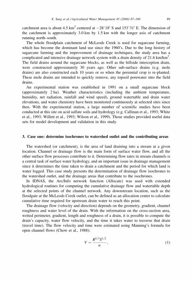
Fig. 1 shows the time of concentration which represent the time required for water to

reach the downstream outlet. The distribution of the time of concentration provides very

useful information in watershed behaviour analysis, as it depicts the speed of

contributions of various parts of the watershed. This is specially the case for non-

homogeneous drainage areas, where the distribution of contributions is not easily

predicted.

4. Case two: assess the capacity of the existing drainage network

Assessment of existing drainage systems or the design of new ones is an important task

for drainage management. The goal is to determine whether an existing drainage network

can adequately convey the flow associated with a designed discharge (or rainfall

intensity). To assess the drainage network conveyance, the discharge produced by the


sub-watershed or cane block is compared to the capacity of the corresponding drainage

network. A rational method is used to estimate the design discharge (Pilgrim, 1987):

Q � 0:278CiA; (2)

where Q is the design discharge (or ¯ow rate, m3/s), i the average rainfall intensity (mm/

h), A the drainage area (km2), C is a runoff coef®cient (dimensionless), the coef®cient

0.278 (� 1/3.6) allows the unit of Q in m3/s when i is in mm/h and A in km2. The runoff

coef®cient is dependent on the character and condition of the soil, slope, and crop, and it

varies with time as crop conditions vary. Thus, reasonable coef®cients must be chosen to

represent the integrated effects of all these factors and their changes over the crop's

phenology.

For each block (polygon), the surface characteristic is assumed uniform. A weighted C

coefficient (C_Value) is assigned to each block according to the variety or land cover

type, and recorded in the polygon attribute table (BLOCK.PAT). In the McLeods Creek

study site, for storm drainage network analysis, 2 and 10 year return period design

discharges are of interest. They are computed using Eq. (2) with the relevant rainfall

intensity.

Fig. 1. Time required for water to reach the downstream center (McLeods Creek outlet).


The rainfall intensity i is calculated from intensity duration frequency (IDF) curves

for the particular area. A method presented by Froehlich (1995) is adopted to obtain

the intermediate IDF equation for the McLeods Creek study site. The generalized form

is:

i � a3

�t � b3�c3; (3)

where i the design rainfall intensity (mm/h); t the rainfall duration (hours); a3, b3 and c3

are parameters which can be determined from the ratio of rainfall depths (24±2 h) and the

return period (years) (Pilgrim, 1987).

The design duration corresponds to the time of concentration (Tc, h), that is, to the

longest time required for units of water, anywhere in the contributing watershed, to arrive

at the point of analysis. The flow time is given by equation (Pilgrim, 1987):

Tc � 0:967L

A0:1S0:2e

; (4)

where L is the stream length (km), and A the block area (km2). Se is the slope of the main

stream (m/km). For each block, L is the diagonal line and it is estimated from the block

perimeter. A is read directly from the polygon attribute table (AREA item) and Se is

calculated from the corresponding elevation items.

Once the design discharge Q entering the OCP pipe has been calculated by the rational

formula, the diameter of pipe D required to carry this discharge can be determined. It is

usually assumed that the pipe is flowing full under gravity but is not pressurized, so the

pipe capacity (Qmax) can be calculated by the Manning's equation. For a full pipe the area

is A � pD2=4, and the hydraulic radius is R � D=4. Thus Manning's equation for pipe

becomes:

Qmax � 0:312

nS1=2D8=3: (5)

This is solved for the required pipe diameter D (m) as:

D � 3:21Qmaxn��Sp

� �3=8

: (6)

The pipe capacity and diameter for 2-year and 10-year return periods were estimated

using Eqs. (5) and (6), and stored in the drain network database. Then, the pipe capacity is

compared with 2-year and 10-year design discharge. A pipe is defined as `problem' or

`undersized' if its capacity (Qmax) is less than the design discharge (Q) of the 2-year

return period. A pipe is defined as `satisfactory' if its capacity is larger than the 10-year

design discharge. A pipe is defined as `borderline' if its capacity (Qmax) is in between 2-

year and 10-year design discharges. Similarly, these comparisons could be made directly

using the pipe diameter instead of capacity, and this provides the users an alternative way

for the pipe capacity assessment. By this means, the problematic pipes can be located and

identified in the database by assigning an identification code in its network attribute table

record.


The results of the conveyance analysis (Fig. 2) shows that out of 400 eligible

pipes, 188 are satisfactory (Qmax > Q10), 121 are deficient (Qmax < Q2), and 91 are

borderline (Q2 < Qc < Q10). This information can then be used by farmers or local

government agents to determine the critical areas that need repair, or use the comparative

Fig. 2. The locations of the de®cient pipes in the McLeods Creek drainage network.


capacities of the method to investigate the impact of the proposed development of a

drainage network.

The computation of cumulative watershed parameters and conveyance checking

involved substantial Arc/Info processing and is fully automated with the AML programs

developed in this study. An alternative approach is an interactive one, where the user

selects from the screen, the pipe they want the computations to be performed for, and the

different assessment criteria (e.g. design discharge for any other return period).

Computations are then performed and the results showing the contributing areas and

the computed values for that pipe are displayed on the screen. The AML program that

performs this process is accessible from the IDNAS under the Network module.

5. Case three: estimate the accumulated acidic pollutant

The export of acidity from ASS sugarcane fields to aquatic ecosystems depends on two

factors: (1) acid existence or production; and (2) discharge of acid soil water (White et al.,

1993). The acid production or the oxidation of pyrite in the soil is highly related to the

dynamics of the watertable positions and soil characteristics, both at the present time and

during the geological past of the last few thousand years. Since most of the surface soils

have already been completely oxidized due to the long drainage history (more than 30

years), the acid production can be regarded as constant over a certain period. Thus, the

acid export or load at a given outlet is only proportional to the discharge capacity and can

be estimated from rainfall, evapotranspiration and block area (Wilson et al., 1999). This

case study estimates the accumulated acidity at the watershed outlet in relation to a given

rainfall event.

If the concentration of H� exported with each outflow is based on a constant pH, then

the mass of sulfuric acid (H2SO4) exported can be calculated for each block or whole

catchment using a simple water balance equation with the areal information from the

block database. A simple linear relationship exists between the outputs of pure sulfuric

acid (Sg) and the volume of discharge (Q) (Sg � aQ � b). The linear coefficient (a) can be

theoretically determined from the antecedent soil pH and the volume discharge using a

chemical mass balance equation. Assuming an average topsoil pH of 3.5, we obtained

a � 0.01549 based on a previous study (Wilson et al., 1999). Note that this coefficient

changes when the soil pH value changes. In practice, a is constant and a negative

intercept (b) is given in the linear equation to account for the tidal intrusion (backwater)

and acid neutralization from its dissolved alkalinity.

If the block or sub-watershed is sufficiently small and the rainfall (P) and

evapotranspiration (ET) are approximately uniform over the affected area At, then over

a certain period (e.g. rainfall period, a day or a month) the discharge of water from the

canefield (blocks) becomes a simple equation (Q � (P ÿ ET)At) (Wilson et al., 1999).

These discharges are then entered into the drainage network system (provided that the

watertable in the field is higher than that in the drain) and conveyed through drains to the

catchment outlet (refer to Figure 3 in Part 1) as presented in the above section (Case 1).

Based on these assumptions, the total contributing area (thus the total pollution load) for a

center (e.g., watershed outlet) at a given period can be obtained by the GIS allocation


process. Using the Allocate routine with, time of concentration as impedance, area as

resource, and the accumulation time as the center's impedance limit, we can obtain a list

of all the drains and the associated cane blocks that drain to that center within the time

limit, and the total contributing area. From that area, the total volume of discharge and the

total pollutant load can be computed (Fig. 3). These processes are implemented in IDNAS

and they are accessible through the Net-Acid program under the Network menu (refer

Figure 6 in Part 1).

The information of accumulated acidity and area is very useful for acid control. For

example, it can be used to calculate how much lime is needed to neutralize the acidity to a

Fig. 3. Accumulated acidic pollutant (sulfuric acid) at McLeods Creek outlet within given times.


certain level for a given area. It can also be used to evaluate the water management

strategies and to develop better management practice, such as the determination of the

most suitable drain spacing. The above analysis can also be extended to predict an acid

outflow event provided the incoming rainfall is known. That is, for a given rainfall event

(rainfall intensity and duration) and known soil water conditions, the total pollutant

loading at the outlet with this rainfall event can be estimated. This provides a means for

the prediction of the possible acid outflow for a specific time and rainfall event.

6. Case four: simulate acid out¯ow events

Outflow events happen if the elevation of the watertable in the cane field is higher than

that of the outflow control point (OCP). Hydrologically, if rainfall duration exceeds the

time of concentration, peak runoff will occur and will influence all the drains. Based on

the observations at the study block, there were 156 rainfall events during the monitoring

period between February 1992 and January 1994. From the point of view of acid drainage

control, typical questions are: (1) does an outflow event happen with a rainfall event? (2)

how much pollutant this rainfall event will bring into the estuary river system? and (3)

what happens to an individual block with each rainfall event? This case study simulates

the acid outflow for the whole catchment, as well as for each cane block, and predicts the

amount of acidic pollutant brought to the outlet for any individual event. This application

is similar to the above one, but it differs in the way that it performs the continuous

simulation by using the IDNAS's spatio-temporal module, and it is in a detailed level for

each block and each rainfall event. Thus, this application can be used for detailed acid

drainage control and management.

To demonstrate the application of the IDNAS spatio-temporal module, this case study

simulates several scenarios of acid outflow events and demonstrates the complete

modelling process based on the system operations. The user activates the program by

typing IDNAS from the ARC prompt and the main menu is then displayed. Once the

Event menu is activated, the user will be prompted to make a series of choices and be

directed to complete the whole process. The process includes these five steps: (a) choose

the time scope and select an interesting rainfall event (e.g., Event 1 on 17/03/1992); (b)

create the initial watertable (WTD0) layer and update watertable (WTD) layer (ET sub-

module and temporal hydrological model are used here); (c) run the network model using

the updated watertable of the simulated event; (d) calibrate the hydrological coefficients

and network settings (e.g. impedance item, variables in the center file); and (e) present

results. Steps 1±5 can be re-processed for another event or the same event without exit the

main program until all events are completed.

When the process has been completed, the user can view the discharge and pollutant

loading for both the whole watershed and an individual block of interest for each event. It

allows the user to analyze the rainfall impacts on the water quality and analyze the

network response to rainfall event (such as pollutant load) at a user-defined site and time.

It can answer the questions such as: how many blocks have outflow, what is the total

area, and how much volume potential water and sulfuric acid are available for discharge?

Fig. 4 displays the potential mass of pure sulfuric acid (H2SO4) with the discharge for


Fig. 4. Event-based simulation of acid discharge at the McLeods Creek study site showing the acid export from

each cane block corresponding to each rainfall event.


individual blocks of selected events. This information can be used to locate the

`problematic' blocks which need to have more attention paid to them for acid control.

7. Discussion and conclusion

This study has demonstrated that the integrated drainage network analysis system

(IDNAS), or in a broad term, the integration of remote sensing, GIS, and hydrological

modelling, is an appropriate tool to facilitate the data management and visualization, to

enhance the efficiency and effectiveness of the simulation models, and to provide options

for better water management for the acid sugarcane land.

The integrated system in this study comprises a variety of data sources for different

processes. The accuracy and consistency of the input data, as well as the analysis models

or methods, determine the quality of the analysis results. Theoretically, perfect simulation

results can be expected if the input data and analytical methods are correct. The

assessment of the overall accuracy of the application (i.e. acid discharge in this study) for

the whole study area should be made at the watershed outlet or other downstream points

of interest. However, the direct measurement of the acid discharge is difficult and such

data are hardly obtainable for the whole catchment. Given this limit, the assessment was

made on a selected field block where intensive field observations of hydrology and soil

were conducted. Thus, simulation accuracy was assessed there for different outflow

events (refer to Fig. 4).

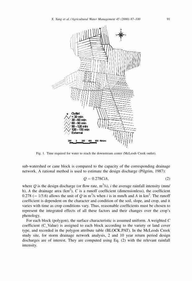
Table 1 compares the simulation results of acid discharge of different outflow events

between model simulation and observation. In Table 1, WT is the watertable elevation

(mm, AHD) by field observation. Discharge is the total amount of water (in volume) in

the soil or drain which was at a position higher than the outflow control point (OCP), thus

was available for discharge. H2SO4 is the mass of pure sulfuric acid contained in such an

amount of discharge. The comparison between the observed and simulated results shows

that the simulation tends to overestimate the discharge and pollutant content (H2SO4)

since the simulation model predicts a higher watertable elevation than that of the

observation. The comparison yields an average error of 7.3% in estimation of the mass of

pure sulfuric acid, with a minimum of 0.9% and a maximum of 12.7%.

Table 1

Comparison between observed and simulated results of acid discharge of different out¯ow events

Event date WT (mm, AHD) Discharge (m3) H2SO4 (t) Relative error(%)

Observed Simulated Observed Simulated Observed Simulated

17/03/92 687 694 8561 8637 133 134 0.9

12/05/92 544 602 7005 7636 109 118 9.0

18/07/92 514 592 6679 7527 104 117 12.7

18/11/92 190 207 3155 3339 49 52 5.9

28/08/93 184 207 3089 3339 48 52 8.1

09/12/93 664 647 8310 8126 129 126 2.2

19/01/94 195 232 3209 3611 50 56 12.5


The watertable position is not only the dominant factor influencing the acidification

and acid flow, but also is the most significant component of error sources, since it is

involved in most of the simulation processes. Although DRAINMOD (Skaggs, 1980) has

been proven as a good tool in simulating the shallow watertables at the study site, great

care needs to be taken when it is used over a large area. To overcome this weakness, a

remote sensing-based method for estimating evapotranspiration and its distribution was

proposed by Yang et al. (1997).

The case studies employed several hydrological methods and models for determination

of hydrological variables. The implementation of the hydrological methods in Arc/Info

does not enhance the methodology per se, but it makes it faster, more accurate, and more

consistent. The main reasons for choosing the relevant hydrological methods (such as the

rational method and Manning's equation) are not only because of their simplicity and

relatively robustness, but also the availability of data (e.g. hydrological coefficients) and

validation of those methods in the study area (e.g. Pilgrim, 1987). However, those

methods can be replaced if more accurate ones are become available in the future.

Through these case studies, it has been demonstrated that the GIS network models and

network analysis routines can be successfully applied to agricultural water resource

management, particularly in a flat floodplain region where natural and artificial drainage

networks define the possible water flows. Using the GIS allocation process capability,

together with embedded external hydrologic modeling and analysis programs, dynamic

simulation of pollutant discharge in the drainage network becomes possible.

The conceptual network model needs to be implemented in an existing GIS

environment. In this study, the current version of Arc/Info software was used. However,

many of the methods developed here can be ported to other GIS environments as long as

there are available, the file exchange and network capabilities. The IDNAS is not limited

to these applications presented in this paper. It could be extended to other applications

such as screening water management plans, liming plans, and tidal intrusion simulation.

A current study is undertaking which implements the IDNAS on a PC-based ArcView

GIS.

The future aims of the study are focused on more complete and precise simulation

methodology of the network, the integration of polygon, grid and network spatial data

models for water and pollutant accumulation and discharge simulation, and developing

the methodology for modeling and monitoring the change of the groundwater elevation of

sugarcane fields in relation to weather and crop conditions with automated field data

loggers and remotely-sensed data. A more precise hydrological model is also to be used

to deal with the backwater problem. Although there is a one-way floodgate at the

connection between estuary water and the field drain, the tidal water influences the field

drain flow and causes the drain water to `̀ back-up'', thus raising the upstream water

surface above normal depth. Backwater calculation is needed to determine the extent of

such effects.

In summary, this study provided a methodology that can be used effectively to simulate

the water balance and drainage network over an agricultural watershed. The system

developed is based on this methodology and can produce informative outcomes for the

estuary users. The success in applying this methodology in acid drainage management,

however, is dependent upon (1) how well the mechanism of the acid drainage and the


hydrological processes are understood; (2) how much and how good is the information

available and necessary for the simulation.

Acknowledgements

This research was sponsored by the Department of Education, Employment, Training

and Youth Affairs (DEETYA) and the Sugar Research and Development Corporation

(SRDC) in Australia. Support was also received from the Charles Sturt University (CSU),

Australia for providing a Postgraduate Writing-Up Award for writing this paper. All of

the sponsorship and support is gratefully acknowledged.

References

Callinan, R.B., Fraser, G.C., Melville, M.D., 1993. Seasonally recurrent ®sh mortalities and ulcerative disease

outbreaks associated with acid sulfate soils in Australian estuaries. In: Dent, D.L., van Mensvoort, M.E.F.

(Eds.), Selected Papers of the Ho Chi Minh City Symposium on Acid Sulfate Soils. Ho Chi Minh City,

Vietnam 2±6 March, 1992. ILRI Publication No.53, International Institute for Land Reclamation and

Improvement, Wageningen, The Netherlands, pp. 403±410.

Chow, V.T., Maidment, D.R., Mays, L.W., 1988. Applied Hydrology. McGraw-Hill, New York, 565 pp.

DeVantier, B.A., Feldman, A.D., 1993. Review of GIS applications in hydrologic modeling. J. Water Resource

Planning and Management 119 (2), 246±261.

Djokic, D., Maidment, D.R., 1993. Application of GIS network routines for water ¯ow and transport. J. Water

Resources Planning and Management 119 (2), 229±245.

Easton, C., 1989. The trouble with the tweed. Fishing World 3, 58±59.

Froehlich, D.C., 1995. Intermediate-duration-rainfall intensity equations. J. Irrigation and Drainage Engineering

(ASCE) 121 (10), 751±756.

Melville, M.D., White, I., Lin, C., 1993. The origins of acid sulfate soils. In: Bush, R. (Ed.), Proceedings of

National Conference on Acid Sulfate Soils, Coolangatta, Queensland, 24±25 June. CSIRO, NSW

Agriculture, Tweed Shire Council, pp. 19±25.

Pilgrim, D.H., 1987. Australian rainfall and runoff: a guide to ¯ood estimation, vol. 1, The Institution of

Engineers, Australia, 374 pp.

Skaggs, R.W., 1980. A water management model for arti®cially drained soils. N.C Agricultural Research

Service, Tech. Bull. No. 267, N.C. State University.

Tunks, M., 1993. Ecological impacts associated with potential acid sulfate soils in the tweed shire. In: Bush, R.

(Ed.), Proceedings of National Conference on Acid Sulfate Soils, Coolangatta, Queensland, 24±25 June.

CSIRO, NSW Agriculture, Tweed Shire Council, 159 p.

White, I., Melville, M.D., Wilson, B.P., Price, C.B., Willett, I.R., 1993. Understanding acid sulfate soils in

canelands. In: Bush, R. (Ed.), Proceedings of National Conference on Acid Sulfate Soils, Coolangatta,

Queensland, 24±25 June. CSIRO, NSW Agriculture, Tweed Shire Council, pp. 130±148.

Willett, I.R., Melville, M.D., White, I., 1993. Acid drainwaters from potential acid sulfate soils and their impact

on estuarine ecosystems. In: Dent, D.L., van Mensvoort, M.E.F. (Eds.), Selected Papers of the Ho Chi Minh

City Symposium on Acid Sulfate Soils. International Institute for Land Reclamation and Improvement,

Publication No. 53, Wageningen, The Netherlands, pp. 419±425.

Wilson, B.P., White, I., Melville, M.D., 1999. Floodplain hydrology, acid discharge and change in water quality

associated with a drained acid sulfate soil. Marine and Freshwater Research 50, 149±157.

Yang, X., Zhou, Q., Melville, M., 1997. Estimating local evapotranspiration of sugarcane ®eld using Landsat

TM Imagery and VITT concept. Int. J. Remote Sensing 18 (2), 453±459.


an integrated drainage network analysis system for ...directory.umm.ac.id/data...

Documents