an integrated spatial decision support system on a ... · thesis submitted to the international...
TRANSCRIPT

An Integrated Spatial Decision Support System on a distributed hydrological model for IWRM in
the semi-arid Nambiyar river basin in India.
Antony Anbarasu Selvaraj March 2009

An Integrated Spatial Decision Support System on a distributed hydrological model for IWRM in the semi-arid
Nambiyar river basin in India.
by
Antony Anbarasu Selvaraj
Thesis submitted to the International Institute for Geo-information Science and Earth Observation in partial fulfilment of the requirements for the degree of Master of Science in Geo-information Science and Earth Observation in Water Resources and Environmental Management with Specialisation: Groundwater Assessment and Management.
Thesis Assessment Board
Name Examiner 1 (Chair) : Prof. Dr. Z. Zu Name Examiner 2 : Prof. O. Batelaan, Vrije Universiteit, Brussels Name Examiner 3 : Drs. R. Becht Name Examiner 4 : Dr. Ir. L.G.J. Boerboom
INTERNATIONAL INSTITUTE FOR GEO-INFORMATION SCIENCE AND EARTH OBSERVATION ENSCHEDE, THE NETHERLANDS

Disclaimer
This document describes work undertaken as part of a programme of study at the International Institute for Geo-information Science and Earth Observation. All views and opinions expressed therein remain the sole responsibility of the author, and do not necessarily represent those of the institute.

i
Abstract
Water management in the semiarid basins of the developing countries has its unique character. Limited water resources on one hand and on the other hand, often inefficient water management supported with very limited tools and skills. Dry spells in these basins are full of problems associated with water assessment, allocation, policy implementation and societal conflicts. This research focuses on the holistic management of a water scarce basin, covering surface water, groundwater and the water management tools.
The surface water resources are assessed at local scale though not dynamic. The dynamic local scale assessment of the groundwater is the core technological problem the basins are facing. A few sets of spread sheet calculations with no regard for the hydrogeological boundaries of the basin is still being followed. The scarce groundwater resource in these semiarid basins gives raise to societal conflicts between the irrigation, industrial and domestic consumption sectors. The basin administrators are often unable to implement their good policies on water sharing for want of a scientific mechanism.
This research is aimed at evolving a framework for groundwater allocation in the basin through a scientifically sound and socially acceptable method. It found the solution in an Integrated Spatial Decision Support System (ISDSS) for the research basin of Nambiyar river in the Tamilnadu state of India. It has a technological engine in its distributed, surface water and groundwater coupled fully transient numerical hydrological model. The social front is in the Collaborative Multi Criteria Decision Making (CMCDM) where all the stakeholders are involved. They consider all the criteria concerning the water utility in the basin and allocate water among themselves as simulated by the hydrological model.
The MIKE SHE code, which covers the entire land phase of the water cycle, is used in the hydrological model. The results of the model qualitatively focus on the output values and it needs further calibration with field test data. The research is a combination of technology put into solvingsocietal conflicts in the water sharing in dry basins.

ii
Acknowledgements
Its my opportunity to gratefully remember all those who are responsible in bringing out this piece of research work along with me. I thank God Almighty who has been with me all these days. I thank the Government of Tamilnadu for sponsoring me to this MSc programme in ITC, Netherlands. I specifically remember the extraordinary interest that Mr. Audi Seshiah, the Principal Secretary to Government (Public works department) took in sending me for this course with a simple and focussed advise that I should do well in my studies and use it for the state of Tamilnadu. I fondly remember the warmth and encouragement that Mr.Ashok Kumar, the Under Secretary of the same unit always extended to me in processing my study proposal.
If I remember the events that led me to this study programme in the chronological order, I thank Mr. Jegatheesan, then Chief Engineer (State Ground & Surface Water Resources Data Centre), PWD, Chennai who recommended my study proposal to the government. I thank Mr. Sundarasekaran, then Engineer-in-Chief, Water Resources Organisation, Chennai who took the initiative of recommending me to the Royal Netherlands Embassy, India for a fellowship which was later negatived. I profoundly thank Mr.Natarajan then Chief Engineer (State Ground & Surface Water Resources Data Centre), PWD, Chennai, India who very optimistically reinitiated my study programme. He just advised me that my study should benefit our country which an euphemism for not to settle in abroad. I thank Mr.Rajagopalan, a senior officer of the World Bank who initiated the process of funding my studies. I am grateful to Mr. Vibu Nair, Project Director, Tamilnadu Irrigated Agriculture Modernisation and Waterbodies Restoration and Management (IAMWARM) Project for proposing my studies under the project he is leading and especially for the positive feedback he gave to the government in the crucial moment with a ‘he deserves to be sent’. I am indebted to the deep involvement that Mr.Thiagarajan, then Chief Engineer (State Ground & Surface Water Resources Data Centre), PWD, Chennai, India took in taking up my study programme at the highest levels of the government with the only expectation in return that I should give him a GIS based hydrological model of my state, Tamilnadu. I thank Mr. Shanmugam, the present Chief Engineer (State Ground & Surface Water Resources Data Centre), PWD, Chennai, India who supported my thesis writing by providing me the hydrogeological & climatic data and facilitating the required infrastructure. I am grateful for my senior engineers, Mr.Nagarajan, and Mr.Rajan for being a source of encouragement to me, especially Mr. Vaidhilingam who encouraged me taking up basin modelling.
I recall and wonder at the amazing warmth and affection that I always received from my teammates, Mr. Muthu Brabhu, Ms.Vidhya, Ms.Easwari, Ms.Meera, Ms.Vardhini, Ms.Vani and Ms.Sudha throughout my studies. I thank my dear colleagues Kathiravan and Chandhuru and especially Vellaichamy for providing me the data in time and technical inputs for my studies. I am overwhelmed by the affection and speed with which I got the field data and photographs from my friend and colleague Mr.Nagarajan. I remember my dear friend Mr.Manmathan whom I often troubled with personal works during my study.
I am very grateful to Mr. Borge Storms of M/s. DHI, Denmark for being instrumental in my thesis. He provided me the expensive MIKE SHE software licence to me till the thesis is complete. He gave me the opportunity to put into action of whatever I learnt from my professors at ITC. I thank Mr.Ajay Pradhan of Ms. DHI, India for accepting me in his office to learn the MIKE SHE software. I thank

iii
Mr. Ajay Sharma, Mr. Nithin, Mr.Acharaj led by Mr. Venkata Rao of Ms.DHI, India for sharing with me their technical knowhow on the MIKE SHE software. I gratefully remember the long late hours that Mr. Ajay Sharma spent with me in this knowledge sharing process.
Finally I remember with extreme gratitude my professors. They all dedicatedly taught me ‘taking decisions on the water resources and environmental management issues with the application of GIS and Remote Sensing’. I tasted the enrichment of professional water resources management from them. Its my desire and duty to carry memories of them with me all through my career. Starting with Mr. Remco, who taught me GIS, Mr.Parodi, who taught me Remote Sensing and Surface Hydrology, Mr.Ben Maathuis, who taught me Remote sensing, Mr. Ambro, who taught me Energy Balance, ETo and basic groundwater, Mr. Chris Mannaerts, who taught me Water Quality and Environmental Management, Mr. Zoltan who taught me Remote Sensing, Mr. Tom Rientjes, who taught me and instilled in me the desire for modelling, Mr. Arno Lieshout, who taught me Crop Water Requirement, Mr. Maciek Lubczynski who taught me Groundwater and Modflow, Mr. Robert Becht who taught me advanced Groundwater and supervised me through my thesis with timely ideas, Mr. Ali Sharifi who taught me Planning Support System & Integrated Water Resources Management, Mr.Johannes Flacke who taught me Planning Support System, Mr. Luc Boerboom who taught me Decision Support Systems & Integrated Water Resources Management supported with lot of demos and site visits and co-supervised my thesis and Prof. Bob Su who with his warm smile and kind enquiries on my studies always encouraged me, all of these professors added value to my career.
I especially thank my supervisors, Mr. Robert Brecht who boldly encouraged me to do the first MIKE SHE model in my institute and Mr. Luc Boer Boom for giving shape to the methodology for water allocation. They showed good understanding in my difficult times when I faced surprises from the complex and sophisticated modelling software. It is their patient and timely support that guided me through the thesis.
Finally, I express my profound gratitude to Mr.Arno Lieshout, Course Director, Water Resources and Environmental Management, ITC for allowing me to take up my thesis in India.

iv
Table of contents
1. Introduction ..................................................................................................................................... 11.1. General ................................................................................................................................... 11.2. Study Area ............................................................................................................................. 11.3. Location ................................................................................................................................. 11.4. Subsoil.................................................................................................................................... 21.5. Irrigation System.................................................................................................................... 21.6. Agricultural Land................................................................................................................... 21.7. Landuse .................................................................................................................................. 21.8. Rainfall................................................................................................................................... 31.9. Socio-economy....................................................................................................................... 31.10. Background and justification ................................................................................................. 31.11. Hydrology .............................................................................................................................. 3
1.11.1. Present assessment of water resources.......................................................................... 41.11.1.1. Surfacewater ............................................................................................................. 41.11.1.2. Groundwater ............................................................................................................. 41.11.1.3. Author’s view on water assessment in the basin ...................................................... 5
1.11.2. Societal Conflicts .......................................................................................................... 51.11.3. Policy making................................................................................................................ 51.11.4. Justification ................................................................................................................... 5
1.12. Research Problems................................................................................................................. 61.13. Research objectives................................................................................................................ 61.14. Research questions................................................................................................................. 61.15. Hypothesis.............................................................................................................................. 6
2. Research Methodology.................................................................................................................... 72.1. Conceptual model .................................................................................................................. 72.2. Hydrological model................................................................................................................ 72.3. ISDSS model.......................................................................................................................... 8
3. MIKE SHE code and Conceptualising the Hydrological model ..................................................... 93.1. Why MIKE SHE .................................................................................................................... 93.2. MIKE SHE in the model...................................................................................................... 103.3. Datatypes in MIKE SHE...................................................................................................... 103.4. Basin specific problems in the conceptualisation of the model........................................... 10
3.4.1. General............................................................................................................................. 103.4.2. Internal boundaries of Irrigation Tanks and Operation of diversion weirs ..................... 103.4.3. Internal boundaries of River ............................................................................................ 113.4.4. Operation of Tank sluices................................................................................................ 113.4.5. Subsoil representation in the hills ................................................................................... 12
4. Data preparation ............................................................................................................................ 134.1. Tools / Primary Data............................................................................................................ 13
4.1.1. Software........................................................................................................................... 134.1.2. GIS Datasets .................................................................................................................... 134.1.3. Climatic data.................................................................................................................... 13

v
4.1.4. Well census data...............................................................................................................134.1.5. Feedback of stakeholders on the use of water..................................................................13
4.2. General data ..........................................................................................................................134.2.1. Nature of Basin.................................................................................................................134.2.2. MIKE SHE data formats ..................................................................................................14
4.3. Topography...........................................................................................................................154.4. Basin boundaries...................................................................................................................154.5. Irrigation Tanks.....................................................................................................................164.6. River......................................................................................................................................164.7. Command Area under Tanks ................................................................................................164.8. Command Area under Irrigation Wells.................................................................................174.9. Pumping wells.......................................................................................................................17
4.9.1. Irrigation wells..................................................................................................................174.9.2. Domestic wells .................................................................................................................184.9.3. Industrial wells .................................................................................................................18
4.10. Subsoil strata and Lithology .................................................................................................184.10.1. Time series data ...........................................................................................................194.10.2. Daily Rainfall ...............................................................................................................194.10.3. Daily Evapotranspiration (ETo)...................................................................................20
4.11. Monthly groundwater levels .................................................................................................205. Modelling steps in MIKE SHE ......................................................................................................22
5.1. Display ..................................................................................................................................225.2. Simulation specification .......................................................................................................225.3. Climate..................................................................................................................................235.4. Landuse:................................................................................................................................235.5. Rivers and Lakes...................................................................................................................235.6. Overland Flow ......................................................................................................................245.7. Unsaturated Flow..................................................................................................................245.8. Saturated Zone ......................................................................................................................245.9. Storing Results......................................................................................................................245.10. Calibration ............................................................................................................................24
5.10.1. Initial manual calibration .............................................................................................255.10.2. Autocalibration.............................................................................................................255.10.3. Initial values .................................................................................................................265.10.4. Autocalibrated values of system parameters................................................................26
5.11. Sensitivity Analysis ..............................................................................................................275.12. Map of residuals ...................................................................................................................275.13. Validation .............................................................................................................................285.14. Uncertainity ..........................................................................................................................28
5.14.1. System parameters .......................................................................................................285.14.1.1. Hydraulic conductivities ..........................................................................................285.14.1.2. Specific yield and Specific storage..........................................................................295.14.1.3. The Conductance of the bed material of the irrigation tank....................................29
5.14.2. Command area under cultivation and ETa...................................................................295.14.3. Pumping wells data ......................................................................................................29

vi
5.14.4. Inflow into irrigation tanks from the river .................................................................. 296. Analysis of Results........................................................................................................................ 30
6.1. Calibration and reliability .................................................................................................... 306.2. Water Balance...................................................................................................................... 316.3. Water Balance Validation.................................................................................................... 32
7. Integrated Spatial Decision Support System (ISDSS)................................................................... 347.1. General ................................................................................................................................. 347.2. Stakeholders ......................................................................................................................... 357.3. Conflicts............................................................................................................................... 367.4. Methodology ........................................................................................................................ 367.5. Collaborative Multi Criteria Decision Making.................................................................... 37
8. Results ........................................................................................................................................... 398.1. General ................................................................................................................................. 398.2. Saturated Zone storage......................................................................................................... 398.3. Evapotranspiration ............................................................................................................... 398.4. Base flow into the river........................................................................................................ 398.5. Research objectives.............................................................................................................. 39
8.5.1. Dynamic local scale assessment of water........................................................................ 398.5.2. Framework for water allocation ...................................................................................... 40
8.6. Further works to be done ..................................................................................................... 409. Executive summary ....................................................................................................................... 4110. References ................................................................................................................................. 4311. Appendix ................................................................................................................................... 44
11.1. Typical Water Balance of the basin..................................................................................... 4411.2. FAO Penman-Motieth Method of calculating ETo. ............................................................ 4511.3. Visuals of Irrigation Tank, Weir, Command area................................................................ 46
vii
List of figures
Figure 1-1: Nambiyar river basin location map .......................................................................................2Figure 2-1: Conceptual Model of the ISDSS ...........................................................................................7Figure 3-1: Hydrologic processes simulated in MIKE SHE ....................................................................9Figure 3-2: River, Reservoir, Weirs and Irrigation Tank System ..........................................................11Figure 3-3: Water Balance of an Irrigation Tank System ......................................................................12Figure 4-1: Groundwater contours on 1 Jan 2001..................................................................................15Figure 4-2: River, Reservoir, Weir and Irrigation Tanks system...........................................................16Figure 4-3: Command Area under Tanks and Wells..............................................................................16Figure 4-4: Irrigation and Domestic Wells ............................................................................................17Figure 4-5: Investigation boreholes........................................................................................................18Figure 4-6: Raingauges ..........................................................................................................................19Figure 4-7: Average quarterly rainfall ...................................................................................................19Figure 4-8: Daily Evapotranspiration.....................................................................................................20Figure 4-9: Raingauges and Piezometers ...............................................................................................20Figure 4-10: Groundwater Hydrographs ................................................................................................21Figure 5-1: Initial results ........................................................................................................................25Figure 5-2: Improved results of autocalibration.....................................................................................27Figure 6-1: Water balance......................................................................................................................31Figure 6-2: Saturated zone storage, Rainfall, ETo in the basin .............................................................32Figure 7-1: Groundwater Allocation Framework on Collaborative Multi Criteria Decision Making...34

viii
List of tables
Table 1-1: Landuse pattern...................................................................................................................... 3Table 1-2: Rainfall pattern ...................................................................................................................... 3Table 1-3: Groundwater assessment criteria ........................................................................................... 4Table 5-1: Initial values of system parameters...................................................................................... 25Table 5-2: Plausible values of system parameters ................................................................................ 26Table 5-3: Auto calibrated values of system parameters ..................................................................... 27Table 5-4: Result of Validation............................................................................................................. 28Table 6-1: Calibration ........................................................................................................................... 30Table 6-2: Expected change in annual saturated zone storage.............................................................. 32Table 6-3: Change in annual saturated zone storage as per the model ................................................. 33Table 7-1: Stakeholders of the basin ..................................................................................................... 35Table 7-2: Stakeholders and conflicts ................................................................................................... 36Table 7-3: Value factors for Multi Criteria as per each shareholder .................................................... 37Table 7-4: Prioritation of monthly water allocation.............................................................................. 38

AN INTEGRATED SPATIAL DECISION SUPPORT SYSTEM ON A DISTRIBUTED HYDROLOGICAL MODEL FOR IWRM IN THE SEMI-ARID NAMBIYAR RIVER BASIN IN INDIA
1
1. Introduction
1.1. General
The people in the semiarid river basins in the developing countries like India face acute water scarcity year by year. The conflicting interests among the domestic, agricultural, industrial and environmental needs on the scarce water resources are ever growing up. This causes socio-economic and ecological problems. After exhausting the limited surface water available during the short monsoon, people depend largely on the groundwater for most part of the year. The solution to this situation is the Integrated Water Resources Management (IWRM) applied at the river basin level.
This situation warrants first the accurate assessment of the surface and groundwater resources of the basin using a surface water and groundwater coupled hydrological model (Maneta et al., 2008). Secondly, the various demand supply scenarios in the basin should be analyzed using an Integrated Spatial Decision Support System (ISDSS) for the judicious spatial and temporal allocation of the water among the stakeholders (Becu et al., 2008). Thirdly, the system should be transparent and induce people’s participation in the decision making process by being easily accessible through a medium like web. This research is such a move in the management of water scarcity in a semiarid river basin.
Modflow code has been extensively used in the groundwater modelling. But it covers the saturated zone only. It needs another code to calculate the groundwater recharge passing through the unsaturated zone. Very few operational level codes have been developed to cover the entire land phase of the hydrological process. MIKE SHE is one such integrated code and has been used in the regional scale hydrological modelling of the Senegal river basin in Africa (Stisen et al., 2008). Since the research basin is semi-arid and the water dynamics in the unsaturated zone is significant, this research uses the MIKE SHE code to study the hydrological behaviour of the basin.
1.2. Study Area
1.3. Location
The study area is the Nambiyar river basin in the Tamilnadu state in the southern part of India. It is a 1046 km² semiarid basin in the hard rock terrain. The Nambiyar is an ephemeral river with stream flows hardly for 2-3 weeks a year. It originates at +1648m MSL in the tropical mountain range, the Western Ghats. It flows on its eastern slopes for 9.6km and enters the plains at about +120m MSL. It further traverses 48km on the plains and joins the sea, Gulf of Mannar. The basin area is 84 km² in the hills and 710 km² in the plain.

AN INTEGRATED SPATIAL DECISION SUPPORT SYSTEM ON A DISTRIBUTED HYDROLOGICAL MODEL FOR IWRM IN THE SEMI-ARID NAMBIYAR RIVER BASIN IN INDIA
2
Figure 1-1: Nambiyar river basin location map
1.4. Subsoil
The basin is of mostly of gneiss except for the coastal sand dunes. The topsoil varies from 0.3m in the western foothills to 10m near the eastern coast. The top soil layer is underlain by weathered gneiss of about 2-10m followed by the fractured gneiss of equal thickness and then the hardrock.
1.5. Irrigation System
The river has 2 medium sized reservoirs and 9 small diversion weirs, feeding to 142 system irrigation tanks (small man-made lakes). Another 80 rainfed irrigation tanks are not connected to the river system. These irrigation tanks are typical of the irrigation system in this part of the world and are several centuries old. They act both as surface water storage and groundwater recharge structures. Shallow dug wells and deep bore wells are predominant and each irrigates an average field size of 1.2ha. In a normal rainfall year, well irrigation is 38%, tank irrigation is 55% and direct river/channel irrigation is just 7% of the gross irrigated area of the basin.
1.6. Agricultural Land
The agricultural land area of 8050ha in the basin is distributed as below, a. System irrigation tanks fed by river = 6179ha b. Nonsystem rainfed irrigation tanks = 1294ha c. Direct river/channel irrigation = 577ha
1.7. Landuse
The following are the 7 land use patterns in the basin. The hills are with tropical forests, mostly because of the rainfall received from the other side of the mountain. The bare soil is predominant and is covered with sporadic patches of drought resistant grass, thorny bushes and Palmyra trees.

AN INTEGRATED SPATIAL DECISION SUPPORT SYSTEM ON A DISTRIBUTED HYDROLOGICAL MODEL FOR IWRM IN THE SEMI-ARID NAMBIYAR RIVER BASIN IN INDIA
3
Table 1-1: Landuse pattern
S.No Land use Area (km²)
% Area
1 Hills 84 10.6%
2 Rock 6 0.8%
3 River 5 0.6%
4 Irrigation Tanks 51 6.4%
5 Command Area_Tanks 54 6.8%
6 Command Area_Wells 7 0.9%
7 Bare soil 587 73.9%
Total Basin Area 794 100%
1.8. Rainfall
The 30 year average rainfall pattern in the basin is given below.
Table 1-2: Rainfall pattern
S.No Seasons Period Rainfall (mm)
%
A South west Monsoon Jun - Sep 39.3 8B North East Monsoon Oct - Dec 289.1 58C Summer Mar - May 138.7 28D Winter Jan - Feb 32.0 6 Total 499.1 100
1.9. Socio-economy
Agriculture is the predominant occupation. The basin covers 61 villages of 100-200 households each and 6 towns of 5000 – 15000 households each. There are few low scale industrial consumers too. A Special Economic Zone, with manufacture of export oriented goods, is under construction in the upper part of the basin. Hence the industrial water demand is expected to shoot up soon.
1.10. Background and justification
This is research is taken up in the backdrop of the following environment.
1.11. Hydrology
The entire basin is on the eastern rain shadow side of the Western Ghats mountain range. The rainfall is non-cyclic in general. Good rainfall occurs only during depressions and cyclones. About 60% of the

AN INTEGRATED SPATIAL DECISION SUPPORT SYSTEM ON A DISTRIBUTED HYDROLOGICAL MODEL FOR IWRM IN THE SEMI-ARID NAMBIYAR RIVER BASIN IN INDIA
4
annual average rainfall occurs during the monsoon (October – December). About 30% rainfall occurs in the summer (March – May) which is mostly lost as evapotranspiration of the order of 6-15mm/day. The irrigation tank system is heavily silted up due to airborne and waterborne silt. This silt reduces the groundwater recharge. The groundwater level has been going down as per local government records.
1.11.1. Present assessment of water resources
1.11.1.1. Surfacewater
The surface water available in the 2 reservoirs is assessed daily. The major contribution of surface water in the basin comes from the vast network of 222 irrigation tanks and it is not assessed dynamically.
A conceptual model called, MRS model, was developed by Dr. Moshe of Ms. Tahal Consulting Engineers, Israel as a part of the World Bank Aided Tamilnadu Water Resources Consolidation Project in the 1990s. It is the first ever model built for the basin and showcased the modelling technology to the state. It is a Conceptual Model of the technology of 1990s and runs on monthly time step with limited consideration for the subsoil lithology.
1.11.1.2. Groundwater
At present the groundwater assessment takes place every five year, which includes a drought, normal and wet year. The basic unit of groundwater assessment is not a natural hydrogeologic boundary. It is an administrative unit called Block, which often transcends hydrogeologic boundaries. The measure of classification of groundwater potential is based on the ‘ratio of abstraction of groundwater to the recharge’ within the basic unit.
Table 1-3: Groundwater assessment criteria
No Category Abstraction/ Recharge
1 Over-exploited >100
2 Critical 90-100
3 Semi-critical 70-90
4 Safe <70
5 Saline Salinity
The assessment is not backed with local scale sub-surface 3D model representing the subsoil. It is not even a conceptual model, but a set of spread sheet calculations with lump sum recharges and subsurface groundwater flows. There are locations with plenty of groundwater within regions classified as groundwater dearth ‘Over-exploited’ regions. The groundwater assessment is neither dynamic nor fully reflecting the real hydrological system at local scale.

AN INTEGRATED SPATIAL DECISION SUPPORT SYSTEM ON A DISTRIBUTED HYDROLOGICAL MODEL FOR IWRM IN THE SEMI-ARID NAMBIYAR RIVER BASIN IN INDIA
5
1.11.1.3. Author’s view on water assessment in the basin
In the author’s opinion, the basin should be modelled with today’s technology, as a Fully Distributed Transient Model having the 3D representation of the surface and subsurface. Also, since the daily evapotranspiration is very high in the basin and the rainfall is sporadic, a model that runs on a Daily Time Step alone can simulate the water dynamics of unsaturated zone well and yield reasonably valid recharge estimates to the saturated zone.
1.11.2. Societal Conflicts
In the wet and normal years, the irrigation tanks are full. The rich farmers near the head reaches and the poor farmers in the tail-end reaches get alike adequate surface water for irrigation.
During dry years, the irrigation tanks are partially filled. Only the rich farmers in the head reaches get surface irrigation water.
During very dry years, the irrigation tanks have no water. Both the rich and poor farmers are left to rely on groundwater only for irrigation.
The rich farmers resort to deepen their dug wells and construct bore wells within their existing shallow dug wells to cope up with the dwindling groundwater table. With the advent of drilling technology, the construction of deep bore wells is on the increase. The poor farmers in the adjoining land parcels could not afford to deepen their wells. Their shallow dug wells go dry. After few consequent dry years, eventually these dry wells get dilapidated and become disused; their agricultural lands become fallow; the poor farmers sell their lands to the rich farmers at the latter’s terms and migrate to towns and cities as job seekers; most of them end up as squatters.
1.11.3. Policy making
Taking stock of the plight of the poor farmers, the government promulgated the “Tamilnadu State Groundwater (Development & Management) Act 2003”. The policy is to control the abstraction of groundwater in those administrative regions where groundwater is declared as ‘over-exploited’, ‘critical’ or ‘saline’ and to allow abstraction only in ‘semi-critical’ and ‘safe’ areas. But the groundwater assessment is neither dynamic nor at local scale. It does not support the policy makers to take informed decision making on water allocation, especially groundwater.
Therefore, even though the government has come out with the policy to regulate groundwater abstraction and the law too has been enacted, it could not be implemented.
1.11.4. Justification
In the backdrop of the above hydrological, social and policy issues, the government feels the need for a research to find out a method to dynamically assess the surface/ groundwater availability in the basin at local scale and to evolve a scientifically sustainable framework to grant water abstraction permits. Hence, this research is directed towards developing a technically sound and socially acceptable Integrated Spatial Decision Supporting System (ISDSS) to assist the government in assessing and granting water abstraction permits.

AN INTEGRATED SPATIAL DECISION SUPPORT SYSTEM ON A DISTRIBUTED HYDROLOGICAL MODEL FOR IWRM IN THE SEMI-ARID NAMBIYAR RIVER BASIN IN INDIA
6
1.12. Research Problems
This research is focused to address the following problems of water scarcity and the related societal conflicts in the basin.
1) The assessment of quantity of water, especially groundwater, is not dynamic at local scale. There are locations with plenty of groundwater within regions classified as groundwater dearth ‘Over-exploited’ regions. This leads to conflicts between the water regulatory agency and the stakeholders seeking permit to abstract water.
2) There is no scientific method to assess and prioritize the water demands of the stakeholders of conflicting interests. This causes random allocation of water resources, often by intuition and experience. Often the head-enders get adequate surface water and the tail-enders are left to fend for themselves with groundwater, if available. This deepens the socio-economic divide and conflicts among the stakeholders of the basin.
1.13. Research objectives
The aim of the research is to develop a method to substantiate the grant of water abstraction permits to the stakeholders of conflicting interests through a dynamic local scale assessment of the spatial and temporal availability of surface/ groundwater in the basin.
The objectives towards this aim are,
1) To develop a method for the dynamic local scale assessment of the spatial and temporal availability of surface water and groundwater in the basin under wet, normal and dry scenarios, using a fully transient surface/ groundwater coupled distributed numerical hydrological model.
2) To develop a water allocation framework for granting water abstraction permits to the stakeholders of conflicting interests, using principles of Collaborative Multi Criteria Decision Making (CMCDM) in an Integrated Spatial Decision Support System (ISDSS).
1.14. Research questions
The following research questions are formulated to achieve the above objectives.
1) How to develop a method for the dynamic local scale assessment of the surface/ groundwater resources in a semiarid river basin which has a unique network of irrigation tanks and wells?
2) How to develop a water allocation framework for granting water abstraction permits to the stakeholders of conflicting interests, using principles of Collaborative Multi Criteria Decision Making (CMCDM)?
1.15. Hypothesis
The following is the hypothesis developed for the research. 1) Modelling the irrigation tanks/ wells at local scale is essential to dynamically assess the
surface/ groundwater resources in the semiarid basin with an annual reference evapo-transpiration of the order of 2900mm.

AN INTEGRATED SPATIAL DECISION SUPPORT SYSTEM ON A DISTRIBUTED HYDROLOGICAL MODEL FOR IWRM IN THE SEMI-ARID NAMBIYAR RIVER BASIN IN INDIA
7
2) The dynamic local scale assessment and conjunctive use of surface/ groundwater is critical for water abstraction regulation to implement Integrated Water Resources Assessment (IWRM) in this semi-arid basin. An Integrated Spatial Decision Support System (ISDSS) with input from the hydrological model and socio economic models is the means to implement IWRM.
2. Research Methodology
2.1. Conceptual model
The integrated spatial decision support system is conceptualised as below.
ISDSS Model
Hydrological Model (MIKE SHE) DTM
Surface features Sub-surface featuresGeo-Database
Supplies (SW+GW)
Scenarios (wet, normal, dry)
Demands (Dom, Irr, Ind)
Alternatives
Decision Rules
Evaluation
Choice Multi-Criteria
SW & GW Spatial / Temporal Distribution
System Parameters Driving forces Modelling
Knowledge System
Figure 2-1: Conceptual Model of the ISDSS
2.2. Hydrological model
Hydrological Model is the heart of the proposed Integrated Spatial Decision Support System (ISDSS). It calculates the spatial and temporal distribution of surface water and groundwater available in the basin under different scenarios of driving forces like rainfall and different demand scenarios like pumping wells. MIKE SHE code is used for the hydrological modelling. It is the state-of-the-art surface water and groundwater coupled distributed fully transient numerical model available in the industry today.
The basin hydrological system is captured in GIS maps and a geo-database. A Digital Terrain Model (DTM) is created as the reference surface. All the surface features like rivers, irrigation tanks, agricultural lands, villages, industrial sites and the subsurface features like the aquifers are added to the model, with the DTM as reference.

AN INTEGRATED SPATIAL DECISION SUPPORT SYSTEM ON A DISTRIBUTED HYDROLOGICAL MODEL FOR IWRM IN THE SEMI-ARID NAMBIYAR RIVER BASIN IN INDIA
8
The system parameters like hydraulic conductivity of soil and driving forces like rainfall are added as attributes to the GIS features. The model is simulated to give the dynamic, local scale, spatial and temporal availability of surface water and groundwater across the basin.
2.3. ISDSS model
An Integrated Spatial Decision Support System (ISDSS) is proposed to generate the alternative uses of water under different scenarios and to select the best choice through Collaborative Multi Criteria Decision Making (CMCDM).
The demand and supply of water under the wet, normal and dry rainfall scenarios are studied. The water use criteria for different demand-supply conditions are input. A set of alternative uses of water under these three scenarios and their impacts are generated. With the help of a Knowledge System (KS) and a set of Decision Rules (DR), the best option of water use at a given location and time is selected.
For the irrigation system in a river basin, Multi Objective Decision Making (MODM) is ideal. But taking into account of the social and technical constraints in implementing the IWRM, the author proposes Multi Attribute Decision Making (MADM), using a set of implementable alternatives, to select the optimum Water Allocation Framework (WAF).

AN INTEGRATED SPATIAL DECISION SUPPORT SYSTEM ON A DISTRIBUTED HYDROLOGICAL MODEL FOR IWRM IN THE SEMI-ARID NAMBIYAR RIVER BASIN IN INDIA
9
3. MIKE SHE code and Conceptualising the Hydrological model
3.1. Why MIKE SHE
MIKE SHE is an integrated modelling code covering the entire land phase of the water cycle. As for as this model is concerned, It covers the rainfall interception, infiltration, overland flow, channel runoff, percolation & interflow in the Unsaturated Zone (UZ), recharge to the Saturated Zone (SZ), groundwater flow into and from the Saturated Zone. It stands out from other industry standard software like Modflow which covers the Saturated Zone only.
Infiltration of precipitation is a very dynamic process. It depends on a complex interaction between precipitations, unsaturated zone soil properties and the current soil moisture content, as well as vegetation properties. The channel runoff and recharge to groundwater are very significantly affected by the dynamic changes in the soil moisture content in the Unsaturated Zone, especially when the rainfall is scanty, sporadic and irregular. MIKE SHE automates the ‘rain to recharge’ process through the Overland and Unsaturated Zone.
Figure 3-1: Hydrologic processes simulated in MIKE SHE
It is exactly this property of MIKE SHE that convinced the author to choose it as the modelling code for the Nambiyar Basin. It is semi-arid; 70% of annual rainfall occurs in just two months (October, November) and the balance spread over the year. To capture the water dynamics going on in the Unsaturated Zone and hence to assess as accurately as possible the recharge to the groundwater, this MIKE SHE code is chosen.
AN INTEGRATED SPATIAL DECISION SUPPORT SYSTEM ON A DISTRIBUTED HYDROLOGICAL MODEL FOR IWRM IN THE SEMI-ARID NAMBIYAR RIVER BASIN IN INDIA
10
3.2. MIKE SHE in the model
The river basin is modelled as a fully distributed finite difference model in the core MIKE SHE code. It covers the entire topography including the irrigation tanks. The main river is modelled as a one dimensional model in the MIKE11 component of the MIKE SHE code. The river is split into segments called river links and the MIKE SHE and MIKE11 are coupled at these river link nodes. The overland flow from the 2D topography and the groundwater flow from the 3D UZ/SZ, exchange water with the river at these river link nodes.
3.3. Datatypes in MIKE SHE
MIKE SHE code has its own data types. The following data types are used in this model.
1) Dfs0: Time series data like precipitation in a station. Data in Excell files are converted to Dfs0 file in the MIKE ZERO Tool Editor.
2) Dfs2: 2 Dimensional grid data like topography; A raster file like .img is converted to Ascii files in ArcGIS and the Ascii files are converted to Dfs2 files in MIKE ZERO Tool Editor.
3) Dfs3: 3 Dimensional grid data like aquifers. In this model, they are created by the MIKE SHE itself from the geological layers and the vertical discretisation specified in the Unsaturated Zone and Computational Layers.
3.4. Basin specific problems in the conceptualisation of the model
The following hydrological problems are encountered in conceptualising the hydrological system in the model.
3.4.1. General
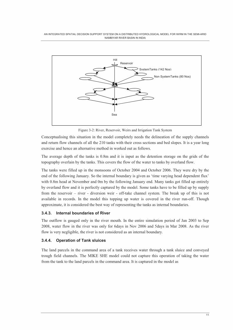
The basin is unique in its nature with 205 irrigation tanks. 142 irrigation tanks receive water from overland flow and also from the river through 11 weirs. The balance 63 irrigation tanks get water from direct overland flow only. Water is stored in the two reservoirs and let into the 142 tanks through the weirs, to top them up. The weir operation is manually controlled. These irrigation tanks are formed in chains, the upstream tank surplusing to the downstream tank and finally into the river. All the 205 irrigation tanks have their own command area for agriculture. There are irrigation wells within these command area. Such a complex irrigation system developed to save every drop of water is very demanding to conceptualise in a model.
The following approach is adopted in conceptualising the model.
3.4.2. Internal boundaries of Irrigation Tanks and Operation of diversion weirs
The 210 irrigation tanks spread across the basin are crucial factors in the recharge of the groundwater. They act as internal boundaries in the model. The water levels in the tanks vary with time. It is at the Full Tank Level (FTL) in the beginning of the monsoon in October and dry just one month after the monsoon ie by the end of January. These tanks receive water directly from the overland flow from rain. They also receive water from the reservoir supplied through the channels off taking from the diversion weirs across the river. Capturing this situation was discussed in detail with the DHI engineer.
AN INTEGRATED SPATIAL DECISION SUPPORT SYSTEM ON A DISTRIBUTED HYDROLOGICAL MODEL FOR IWRM IN THE SEMI-ARID NAMBIYAR RIVER BASIN IN INDIA
11
Figure 3-2: River, Reservoir, Weirs and Irrigation Tank System
Conceptualising this situation in the model completely needs the delineation of the supply channels and return flow channels of all the 210 tanks with their cross sections and bed slopes. It is a year long exercise and hence an alternative method in worked out as follows.
The average depth of the tanks is 0.8m and it is input as the detention storage on the grids of the topography overlain by the tanks. This covers the flow of the water to tanks by overland flow.
The tanks were filled up in the monsoons of October 2004 and October 2006. They were dry by the end of the following January. So the internal boundary is given as ‘time varying head dependent flux’ with 0.8m head at November and 0m by the following January end. Many tanks got filled up entirely by overland flow and it is perfectly captured by the model. Some tanks have to be filled up by supply from the reservoir – river - diversion weir - off-take channel system. The break up of this is not available in records. In the model this topping up water is covered in the river run-off. Though approximate, it is considered the best way of representing the tanks as internal boundaries.
3.4.3. Internal boundaries of River
The outflow is gauged only in the river mouth. In the entire simulation period of Jan 2003 to Sep 2008, water flow in the river was only for 6days in Nov 2006 and 5days in Mar 2008. As the river flow is very negligible, the river is not considered as an internal boundary.
3.4.4. Operation of Tank sluices
The land parcels in the command area of a tank receives water through a tank sluice and conveyed trough field channels. The MIKE SHE model could not capture this operation of taking the water from the tank to the land parcels in the command area. It is captured in the model as
Reservoir
Non SystemTanks (80 Nos)
SystemTanks (142 Nos)
Sea
Hill

AN INTEGRATED SPATIAL DECISION SUPPORT SYSTEM ON A DISTRIBUTED HYDROLOGICAL MODEL FOR IWRM IN THE SEMI-ARID NAMBIYAR RIVER BASIN IN INDIA
12
Figure 3-3: Water Balance of an Irrigation Tank System
During the crop period of 3months, the following activities take place in an irrigation tank system.
1) Continuous overland inflow and onetime river supply into the tank.
2) Evaporation and infiltration from the tank’s water spread area.
3) Tank sluice supply to the command area.
4) Evapotranspiration and infiltration from the command area.
Inflow into tank = Evaporation + Infiltration from tank + sluice supply
Tank sluice supply = Actual Evapotranspiration + Infiltration
All these activities are captured by MIKE SHE, except the tank sluice supply and the onetime river supply into the tanks. The one time river supply is explained above. Only thing is that they are not coupled to the tank sluice supply and the consequent reduction in the water level in the tank. It is approximated in the model by providing a time varying internal boundary to the water level in the tank from 0.8m to 0m in a period of 4 months, which is the field condition.
3.4.5. Subsoil representation in the hills
The investigation boreholes were available only in the plain and not on the hills obviously. The topography layer is directly available from the DEM. The bottoms of topsoil, weathered gneiss and fractured gneiss were interpolated with the basin boundary as the masking extent. This resulted in a reduced level of the bottom of topsoil at 174m only under the mountain. It is preposterous for a mountain of 1652m high. The MIKE SHE code too expected exorbitant depths of unsaturated zone under the mountain.
Hence, the thickness of the topsoil, weathered gneiss and fractured gneiss under the mountain alone, is assumed as 3m each. The bottoms of topsoil, weathered gneiss and fractured gneiss are derived from the DEM using raster calculation in ArcGIS. These layers under the mountains are then mosaiced with the interpolated layers in the plain. This arrangement is a reasonable representation of the hydrological situation.
Evaporation
Infiltration Tank
Sluice supply
Evapotranspiratio
Infiltration CA
Overland flow (continuous) + River supply (one time)
Irrigation Tank

AN INTEGRATED SPATIAL DECISION SUPPORT SYSTEM ON A DISTRIBUTED HYDROLOGICAL MODEL FOR IWRM IN THE SEMI-ARID NAMBIYAR RIVER BASIN IN INDIA
13
4. Data preparation
4.1. Tools / Primary Data
The following software tools and basic data are used in the input data preparation for the model.
4.1.1. Software
The ArcGIS 9.2, Erdas Imagine and MIKE SHE 2008 are used.
4.1.2. GIS Datasets
30m resolution Aster DEM imageries and the Toposheets of Survey of India are used. Other GIS data sets are developed by the author.
4.1.3. Climatic data
The following data are available for the entire simulation period of Jan 2003 to Sep 2008. Daily climatic data is available from one climatic station. Daily rainfall data is available from …rainfall stations. Monthly groundwater level data are available from 12 piezometers. Xxx Investigation borehole data with the lithology data are available. The daily river discharge data at the river mouth is available.
4.1.4. Well census data
A physical count of all the wells in the state was initiated by the local government in 2004. The number of irrigation wells, domestic wells and industrial wells along with their related data like command area are available.
4.1.5. Feedback of stakeholders on the use of water
The feedback of stakeholders on the use of surface water and groundwater in the dry, normal and wet scenarios are obtained.
4.2. General data
Data preparation is a real mammoth job encountered in this model building. The complexities are both because of the unique nature of the research basin as well as the MIKE SHE code.
4.2.1. Nature of Basin
The research basin is a unique irrigation system depicting a typical irrigation system in the southern part of India. The following are the datasets prepared for this model.
GIS Datasets1) Polygon shape file of the riverbasin boundary and the river.
2) Polygon shape files of 205 irrigation tanks with their attribute data like command area and capacity.
3) Polygon shape files of command areas of these 205 irrigation tanks. These maps are prepared as rectangular polygons of area equal to the extent of command area.

AN INTEGRATED SPATIAL DECISION SUPPORT SYSTEM ON A DISTRIBUTED HYDROLOGICAL MODEL FOR IWRM IN THE SEMI-ARID NAMBIYAR RIVER BASIN IN INDIA
14
4) Polygon shape file of the command area under the wells within the command area of these 205 tanks.
5) Polygon shape file of the Theisson polygons for raingauges.
6) Point shape file of the irrigation pumping wells in these command areas under wells.
7) Point shape file of the domestic pumping wells in the 61 villages in the basin.
8) Point shape file of the 11 raingauges in the basin.
9) Point shape file of the 11 piezometers in the basin.
10) Point shape file of the 50+ Investigation boreholes for lithology.
11) DEM of the basin mosaiced from 6 imageries.
12) Raster map of the bottom of the Top soil from the point data of the Investigation boreholes.
13) Raster map of the bottom of the Weathered Gneiss from the point data of the Investigation boreholes.
14) Raster map of the bottom of the Fractured Gneiss from the point data of the Investigation boreholes.
15) Raster map of the initial groundwater table from the piezometric GWL data.
Time series Data:The following time series data are prepared for the entire simulation period from 1 Jan 2003 to 30 Sep 2008.
1) Daily reference evapotranspiration ETo, from the daily temperature, sunshine hours, wet/dry bulb temperatures, wind speed data.
2) Daily Rainfall data for the 11 raingauges in and adjacent to the basin.
3) Monthly groundwater level data for the 11 piezometers.
4) Daily pumping rate for 205 representative irrigation wells under the irrigation tanks.
5) Daily pumping rate for 61 representative domestic wells in the villages.
6) Daily water level in the irrigation tanks for the internal boundaries.
7) Daily Leaf Area Index (LAI) and Root Depth (RD) for the vegetation types namely, forest, grass in bare soil, command area under the tank and the command area under the wells.
4.2.2. MIKE SHE data formats
MIKE SHE has its own following unique datatype formats.
1) Dfs0: Time series data like precipitation in a station. Data in Excell files are converted to Dfs0 file in the MIKE ZERO Tool Editor.
2) Dfs2: 2 Dimensional grid data like topography; A raster file like .img is converted to Ascii files in ArcGIS and the Ascii files are converted to Dfs2 files in MIKE ZERO Tool Editor.

AN INTEGRATED SPATIAL DECISION SUPPORT SYSTEM ON A DISTRIBUTED HYDROLOGICAL MODEL FOR IWRM IN THE SEMI-ARID NAMBIYAR RIVER BASIN IN INDIA
15
Almost all the above GIS datasets need to be converted into Dfs2 format and the time series data be converted into Dfs0 format before feeding them into the model.
4.3. Topography
A Digital Elevation Model (DEM) is created for the purpose of acting as a reference surface for both the surface and subsurface features. It facilities the gravity flow of water in the model, both on the surface and subsurface.
30m x 30m resolution DEM from Aster imageries covering the Nambiyar basin is used. The individual scenes are mosaiced using ERDAS. The altitudes range from 0 at the eastern sea level to +1652 m at the western mountains. Calibrating the DEM using the Differential GPS (DGPS) points was not done. Rather the concept of relative reduced levels with the elevation value at sea as zero was adopted. The bore log lithology and the groundwater levels are pegged to the DEM and hence the approach is justified.
4.4. Basin boundaries
To capture the water balance as accurately as possible defining the model boundaries is critical. The boundaries are in two categories, namely the Surface water and Groundwater boundaries.
Surface water boundaries:The digitized Survey of India toposheets are used to delineate the surface water divide of the basin. The zones where the streams originate and flow in the opposite directions define the surface water divide. The sea is the basin boundary on the eastern side. The surface water divide defines the basin boundaries on the remaining western, northern and southern sides.
Groundwater boundaries:
30
2040
50
60
10
70
80
90
0
100
100
20
0
30
10
0
1 00
Figure 4-1: Groundwater contours on 1 Jan 2001
In general the groundwater divide follows the surface water divide. I used the piezometric groundwater level data to confirm this in this model. I plotted the 1m interval contours of the groundwater levels as on 01 Jan 2001 in the Nambiyar basin and the adjoining two basins in ArcGIS. I drew the flow lines normal to the equipotential lines of groundwater. The flow lines do not intersect the surface water divide except in a small stretch in the northern surface water divide near the sea. This stretch is a sand dune and is very small and negligible.
Thus it is confirmed that the groundwater divide follows the surface water divide of the basin.

AN INTEGRATED SPATIAL DECISION SUPPORT SYSTEM ON A DISTRIBUTED HYDROLOGICAL MODEL FOR IWRM IN THE SEMI-ARID NAMBIYAR RIVER BASIN IN INDIA
16
4.5. Irrigation Tanks
The Nambiyar basin has 222 irrigation tanks. 142 tanks are connected to the river by supply channels and the remaining 80 are rainfed irrigation tanks unconnected to the river. Of these, all the 142 system tanks and 53 major rainfed tanks are included in the model. The remaining 17 rainfed tanks are very small in size and are hydrologically not so significant.
These 205 irrigation tanks were available as just polygon features without attribute data. The related attribute data like storage capacity at Full Tank Level (FTL) and the Command Area (CA) of agricultural land under each tank are added to the ArcGIS maps. The total storage capacity of all the tanks is 36million cubic meters (MCM).
Figure 4-2: River, Reservoir, Weir and Irrigation Tanks system
4.6. River
The river is a polygon feature as the width of the river is about 100m.
4.7. Command Area under Tanks
The command areas under the tanks are not available in the form of digital maps. They are available as chain surveyed paper maps. Digitizing these paper maps and georeferencing them for all the 205 tanks need considerable time. The purpose of bringing these command area into the model is to account for the evapotranspiration and infiltration from the cultivated land.
Weir1
�LAND USE MAP
LandusesBaresoilCAtanksCAwellsHillsRiverRockTanks
0 2 4 6 81Kilometers
Figure 4-3: Command Area under Tanks and Wells

AN INTEGRATED SPATIAL DECISION SUPPORT SYSTEM ON A DISTRIBUTED HYDROLOGICAL MODEL FOR IWRM IN THE SEMI-ARID NAMBIYAR RIVER BASIN IN INDIA
17
It is accomplished by creating rectangular annular polygons downstream of each tank with area equal to their command area as available in the chain surveyed paper maps. Hydrologically it is justified as for as the distributed model is concerned.
4.8. Command Area under Irrigation Wells
There are about 20 to 30 irrigation wells under the command area of each tank. Each well commands about 0.5 to 1 ha of land. When the irrigation tanks are filled up these lands are surface irrigated with the water in the tanks. When the tanks are partially filled or dry, they are well irrigated with groundwater. Digitised maps of these command area under well irrigation is not available. They constitute about 12% of the total command area under the tanks as found out from the well census done by the local government in 2004.
The command area under the irrigation wells are represented as square polygons of 12% of the area of the command area under the tanks. They fit inside the annular polygons of the command area under the tanks. This representation is hydrologically justified as in the case of the command area under tanks.
4.9. Pumping wells
The groundwater is abstracted both by the Irrigation Wells in the command area and the domestic wells spread across the villages. The local government has done a survey of all the wells in 2004. Each village has about 20-60 domestic wells. There are about 20-30 irrigation wells in each command area. It is too detail to represent them individually in the model.
�
�
��
�
��
�
�
��
�
�
�
�
�
� �
��
� �
�
����������
��
�
�
�
��
�
�
�
�� �
��
�
�
���
�
�
���
�
�
��
�
��
���
�
�
�
� ��
� �
��
�
���
�
�
� �
� �
�� �
��
�
�
�
�
�����
���
�������
�
� �
����
�
�
�
�
� ��
�
���
��
��
��
��
�
��
� ���
�
��
� ��
�
�
��
��
�
��
�
�
�
�
��
�
���
�
�
�
�
��
��
���
�
� ��
��
�
�
�
�
�
�
��
� ��
�� �
�
��
�
�
Weir1
�IRRIGATION & DOMESTIC WELLS
� NambiyarIrrigationWells
NambiyarDomesticWells
0 2.5 5 7.5 101.25Kilometers
Figure 4-4: Irrigation and Domestic Wells
4.9.1. Irrigation wells
All the wells in the command area under each tank are represented with one irrigation well at the centre of the command area. Its pumping rate is derived from the irrigation requirement of the crop as below.
Daily pumping rate = A x D / P crop period
Where, A = Area of command area (sq.m) D = Irrigation requirement for the entire crop period (m) P = crop period (days)

AN INTEGRATED SPATIAL DECISION SUPPORT SYSTEM ON A DISTRIBUTED HYDROLOGICAL MODEL FOR IWRM IN THE SEMI-ARID NAMBIYAR RIVER BASIN IN INDIA
18
4.9.2. Domestic wells
All the domestic wells in a village are represented with one domestic well at the centre of the village. Its pumping rate is derived at the rate of 3000m3 per well per day.
As there are 142 command areas of tanks and 61 villages spread across the basin, there is a fair distribution of abstraction across the basin and the representative wells is hydrologically justified.
4.9.3. Industrial wells
There are no heavy industries consuming large abstractions in the basin. Data on the spatially distributed small and medium industrial wells are not available. Their effect on the abstraction of groundwater is parcelled along with the domestic wells.
4.10. Subsoil strata and Lithology
The local government has been drilling investigation borehole in the basin since 1972. There are 47 nos of investigation boreholes in the Nambiyar basin and 82 nos in the adjacent basins. These investigation boreholes were drilled up to hard rock. These lithologies are grouped into topsoil, weathered gneiss and fractured gneiss for the purpose of modelling.
�
�
�
�
�
�
�
��
�
�
�
�
�
�
�
��
��
�
�
�
�
�
�
�
�
�
�
�
�
�
�
�
�
�
�
�
�
�
�
� �
�
�
�
�
�
�
�
�
�
�
�
�
�
�
�
�
��
�
�
�
�
�
�
�
�
�
�
�
��
�
��
Weir1
9
8
7
6
5
4
3
1
9392
91
9089
88
87
8584
83
82
81
80
78
77
75
74 73
72
71
70
69
67
66
65
64
6362
61
60
59
58
57
56
5453
51
50
49
48
47
45
44
43
42
41
39
38
37
36
34
33
31
30
29
27
26
2321
2019
18
17
16
1514
13
12
10
�LITHOLOGY BORE HOLES
0 5 102.5 Kilometers
Figure 4-5: Investigation boreholes
The investigation boreholes have their latitude / longitude and also the elevation above mean sea level (amsl) measured from the local datum. But the elevation should have a common reference surface. Hence, these boreholes were overlaid against the DEM and their elevation at ground level were found out and used in the model.
The reduced level of the bottoms of the Topsoil, weathered Gneiss and Fractured Gneiss were worked out in Excell; Point maps of these bottom levels were plotted in ArcGIS; The point maps were converted to raster maps in ArcGIS using ‘Inverse Distance Weighted’.
Thus the following four raster layers are prepared.
1) Topography ie ground level

AN INTEGRATED SPATIAL DECISION SUPPORT SYSTEM ON A DISTRIBUTED HYDROLOGICAL MODEL FOR IWRM IN THE SEMI-ARID NAMBIYAR RIVER BASIN IN INDIA
19
2) Bottom of Topsoil
3) Bottom of Weathered Gneiss
4) Bottom of Fractured Gneiss ie hard rock.
4.10.1. Time series data
The following major time series data are used in this model.
1) Daily rainfall data from 11 rainfall stations.
2) Daily evapotranspiration data from one climatic station.
3) Monthly groundwater levels from 11 piezometers.
4.10.2. Daily Rainfall
Daily rainfall data from 4 stations within the basin and 7 stations in the adjacent basins are available from 1991 but used from 2003 onwards.
Weir1
Erwadi
Kalakad
Panagudi
Nanguneri
Moolapatti
Radhapuram
Sathankulam
Nambiyar Res
Aralvoymozhi
KulasekarapatnamVijayanarayanapuram
�RAIN GAUGES
Raingauge
RainZone
0 2.5 5 7.5 101.25Kilometers
Figure 4-6: Raingauges
RAINFALL - QUARTERLY
0
100
200
300
400
500
600
Mar-03
Jun-03
Sep-03
Dec-03
Mar-04
Jun-04
Sep-04
Dec-04
Mar-05
Jun-05
Sep-05
Dec-05
Mar-06
Jun-06
Sep-06
Dec-06
Mar-07
Jun-07
Sep-07
Dec-07
Mar-08
Jun-08
Sep-08
Rainf
all m
m
Qtr Avg RF Normal
Figure 4-7: Average quarterly rainfall
The average rainfall pattern of the basin indicates major rainfall during the North-east monsoon during October – December. There is also a sizable summer rainfall during March – May. Few data gaps in the stations are filled with the rainfall data from the station in the immediate proximity.

AN INTEGRATED SPATIAL DECISION SUPPORT SYSTEM ON A DISTRIBUTED HYDROLOGICAL MODEL FOR IWRM IN THE SEMI-ARID NAMBIYAR RIVER BASIN IN INDIA
20
4.10.3. Daily Evapotranspiration (ETo)
There is only one climatic station in the basin at Aralvoymozhi, just on the southern side of the basin. Maximum/ minimum temperatures, dry bulb/ wet bulb temperatures, wind speed, sunshine hours and rainfall are recorded on daily basis since 1991. The daily Reference Crop Evapotranspiration (Eto) was calculated using the FAO: 56 Guidelines for calculating the daily ETo.
Daily Eto
02468
10121416
1/1/
03
1/1/
04
1/1/
05
1/1/
06
1/1/
07
1/1/
08
Dai
ly E
to m
m
Figure 4-8: Daily Evapotranspiration
4.11. Monthly groundwater levels
�
�
��
�
�
�
�
�
�
�
Weir1
93065
93063
93062
93061
93041
93032
93031
27047D
27042D27041D
27028D
27026D
93032AErwadi
Kalakad
Panagudi
Palamore
Nanguneri
Moolapatti
Radhapuram
Sathankulam
Nambiyar Res
Aralvoymozhi
Vijayanarayanapuram
�RAINGAUGES & PIEZOMETERS
� NambiyarRainGauges
NambiyarSubPiezo
0 2.5 5 7.5 101.25Kilometers
Figure 4-9: Raingauges and Piezometers

AN INTEGRATED SPATIAL DECISION SUPPORT SYSTEM ON A DISTRIBUTED HYDROLOGICAL MODEL FOR IWRM IN THE SEMI-ARID NAMBIYAR RIVER BASIN IN INDIA
21
Foothills Fluctuation: 3m
Plain Fluctuation: 20m
Sea coast Fluctuation: 4m
Figure 4-10: Groundwater Hydrographs
The groundwater level in the basin is recorded on monthly basis in 12 piezometers. A typical groundwater hydrograph as input into the model is shown here. They vary from an annual fluctuation of 4m to 16m. Few spikes were noted in the groundwater hydrograph. They are due to typographical errors and are rectified.

AN INTEGRATED SPATIAL DECISION SUPPORT SYSTEM ON A DISTRIBUTED HYDROLOGICAL MODEL FOR IWRM IN THE SEMI-ARID NAMBIYAR RIVER BASIN IN INDIA
22
5. Modelling steps in MIKE SHE
The following are the modelling steps in the interface of MIKE SHE.
5.1. Display
The GIS maps of the basin are shown as a background template.
5.2. Simulation specification
Under the simulation specification, the following specifications are defined for the water movement model.
1) Overland Flow: Finite Difference option is selected.
2) Rivers and Lakes: This option is selected to include the river as a one dimensional model under MIKE11 component.
3) Unsaturated Flow: Gravity Flow option is selected because the Richards Equation option requires about 307hrs for one simulation run. The Gravity Flow option considers the potential head only whereas the Richards equation considers the soil matrix pressure head too.
4) Evapotranspiration: This option is selected as it is mandatory for Unsaturated Zone calculations.
5) Saturated Flow (SZ): Finite Difference option is selected, ignoring the conceptual Linear Reservoir option, as groundwater estimation at local scale is required.
6) Advection Dispersion (AD) Water Quality: This option is not selected as the water quality aspects are not targeted.
7) Simulation Title: Sim1_ddmmyyyy is given as title.
8) Simulation Period: 1 Jan 2003 to 30 Sep 2007 is given as simulation period. 2003 is a drought year and so a preferred start-up time for the model. 1 Oct 2007 to 30 Sep 2008 is reserved for validation.
9) Time Step Control:
a. Initial Time Step: 24hrs
b. Max allowed Over Land Time Step: 0.5 hrs.
c. Max allowed Unsaturated Zone Time Step: 2 hrs
d. Max allowed Saturated Zone Time Step: 24 hrs
10) Over Land Computational Control Parameters:
a. Solver: Explicit Solver is selected with maximum Courant Number of 0.8.
b. Common Stability Parameters: 0.1mm Threshold water depth for overland flow and 0.001 Threshold gradient for applying low gradient flow reduction are selected.

AN INTEGRATED SPATIAL DECISION SUPPORT SYSTEM ON A DISTRIBUTED HYDROLOGICAL MODEL FOR IWRM IN THE SEMI-ARID NAMBIYAR RIVER BASIN IN INDIA
23
c. Over Land – River exchange Calculation: Manning equation is selected.
11) Unsaturated Zone Computational Control Parameters:
a. Calculations in all grid cells are selected.
b. Green and Ampt Infiltration Method is selected.
c. Initial condition: Equilibrium pressure profile is selected.
d. UZ-SZ coupling control: Max profile water balance error of 1mm is selected.
12) Saturated Zone Computational Control Parameters:
a. Solver Type: Preconditioned Conjugate Gradient, Transient solver is selected.
b. Iteration Control: Max number of iterations as 70, Max head change per iteration as 5mm and Max residual error as 0.5mm/day are specified.
c. Sink de-activation in drying cells: Saturated thickness threshold of 50mm is specified.
13) Model Domain and Grid : The origin and grid size are specified in meters. 90m Grid size represented the irrigation tanks nicely, but it took exorbitant time of 40 hours for running the model. 900m Grid makes the model run in 4.5 hours, but could not represent the irrigation tanks satisfactorily. As a balanced size, 500m Grid is provided. It covers smaller tanks at least in one grid and takes an affordable 14hours run time.
14) Topography: It is the raster reference surface for all the vertically dimensioned entities like, depths of irrigation tanks, slope for Over Land flow, subsoil layers and bottom boundary. 30m resolution ASTER DEM is used as the topography.
5.3. Climate
1) Precipitation: There are 9 raingauges in the basin. A shape file of the theisson polygons covering the raingauges determines the spatial distribution of rainfall in the basin. Each polygon is attached to a time series file of daily rainfall.
2) Evapotranspiration: One climatic station represents the basin. So the reference evapotranspiration is applied uniform across the basin. It is attached to a time series file of daily ETo.
5.4. Landuse:
Vegetation: A raster map of the cropped area, viz. Hill, Bare soil Command Area under Tanks and Command Area under Wells is added. LAI and Root Depth values are attached as constant values for the Hill / Bare soil and as a time series for both the Command areas.
5.5. Rivers and Lakes
The MIKE11 simulation file for the river runoff is attached to the MIKE SHE at this point. This simulation file contains a river network digitised from the MIKE SHE river map, cross sections and initial flow at the 0 chainage, Few tick marks during digitising are selected as the river link nodes to connect the one dimensional MIKE 11 with the 2D/3D MIKE SHE.

AN INTEGRATED SPATIAL DECISION SUPPORT SYSTEM ON A DISTRIBUTED HYDROLOGICAL MODEL FOR IWRM IN THE SEMI-ARID NAMBIYAR RIVER BASIN IN INDIA
24
5.6. Overland Flow
1) Manning Number:The overland flow is governed by the Manning’s equation. The Manning’s coefficient (1/n) of 30 is applied.
2) Detention Storage:Detention Storage is a value assigned to every grid in the model topography. 800mm is assigned for the irrigation tanks and 1mm for other areas. During the simulation, if the accumulated overland flow in a grid exceeds, these values, then the overland flow to the next downstream grid starts.
3) Initial water Depth:It is the initial depth of surface water on the topography of the model. Since the simulation period starts on 01 Jan 2003 which is a dry spell, a value of 0mm is assigned.
5.7. Unsaturated Flow
Unsaturated flow is the water movement below the topography upto the prevailing groundwater table. It covers all the three layers, namely Top soil, weathered Gneiss and Fractured Gneiss. The downward flow of water is very dynamic in this zone and is much influenced by the vertical grid discretisation. Very small layer thicknesses of 5mm are given near the ground surface and gradually increased to 10mm, 20mm, 50mm down below.
5.8. Saturated Zone
The saturated zone is the place where the geological layers, Top soil, Weathered Gneiss and Fractured Gneiss are represented in the model. Each of these layers has the following four details.
1) Horizontal hydraulic conductivity (Kh)
2) Vertical hydraulic conductivity (Kv)
3) Specific yield (Sy)
4) Specific storage (Ss)
5.9. Storing Results
The simulation outputs are stored in exclusively as the following types,
1) Time series files like GWLs in piezometers.
2) MIKE 11 river discharge as time series files.
3) Grid data files like evapotranspiration and water head in saturated zone grids.
5.10. Calibration
The RMSE, R and R² between the simulated and observed groundwater levels in the 11 piezometers in the basin and river flows at outlet are used as objective functions for calibration. Initially the calibration was done manually by changing the system parameters to narrow down to the plausible range of values. Then the likely range of these system parameters are input into the model, to run the auto calibration (Henriksen et al., 2003).

AN INTEGRATED SPATIAL DECISION SUPPORT SYSTEM ON A DISTRIBUTED HYDROLOGICAL MODEL FOR IWRM IN THE SEMI-ARID NAMBIYAR RIVER BASIN IN INDIA
25
5.10.1. Initial manual calibration
The following major system parameters are calibrated with the initial values as below.
Table 5-1: Initial values of system parameters
S.No
Parameter Sym
Unit Inceptisol
Alfisol Entisol Forestsoil
Weat.Gneiss
Frac Gneiss
1 Horizontal hydraulic conductivity
Kh m/d 3 10 20 22 5 2
2 Vertical hydraulic conductivity
Kv m/d 0.3 1 2 2.2 0.5 0.2
3 Specific yield Sy (-) 0.15 0.18 0.2 0.22 0.06 0.02
4 Specific storage Ss 1/m 1.5e-4 1.2e-4 1.0e-4 1.3e-4 1.0e-4 1.0e-4
5 Conductance of tank bed
m²/d 0.01 0.01 0.01 0.01 - -
6 Manning’s Number(1/n)
M 30 30 30 30 - -
The model output showed the following typical results.
Figure 5-1: Initial results
The results were not satisfactory and the auto calibration was run to get a better correlation between the observed and simulated state variables.
5.10.2. Autocalibration
The manual calibration of the model takes exorbitant time for each run of about 11hours. Further the system parameters are also not fully based on field tests. Only likely ranges of the system parameters

AN INTEGRATED SPATIAL DECISION SUPPORT SYSTEM ON A DISTRIBUTED HYDROLOGICAL MODEL FOR IWRM IN THE SEMI-ARID NAMBIYAR RIVER BASIN IN INDIA
26
are used in the model. Hence, it is decided to run the auto calibration of the MIKE SHE code to calibrate the system parameters of the model.
The auto calibration is based on the Shuffled Complex Evaluation Method. The following are the criteria for the auto calibration.
a) Number of iterations = 50
b) Loop = 3
c) Minimum relative change in objective function value = 0.01
5.10.3. Initial values
To run the autocorrelation, the following initial and plausible ranges of values are given. Table 5-2: Plausible values of system parameters
S.No Parameter Symbol Unit Initial value
Lower bound
Upper bound
1 Topsoil 1.1 Horizontal hydraulic
conductivity TS_Kh m/d 25.5 3 60
1.2 Vertical hydraulic conductivity
TS_Kv m/d 0.556 0.1 3
1.3 Specific yield TS_Sy (-) 0.116 0.08 0.3 1.4 Specific storage TS_Ss 1/m 0.000129 0.1e-05 0.0005 2 Weathered Gneiss 2.1 Horizontal hydraulic
conductivity GW_Kh m/d 5.19 1 10
2.2 Vertical hydraulic conductivity
GW_Kv m/d 0.665 0.1 1
2.3 Specific yield GW_Sy (-) 0.0838 0.02 0.3 2.4 Specific storage GE_Ss 1/m 0.0000952 0.5e-04 0.0005 3 Fractured Gneiss 3.1 Horizontal hydraulic
conductivity GF_Kh m/d 4.65 0.5 10
3.2 Vertical hydraulic conductivity
GF_Kv m/d 0.16 0.05 0.3
3.3 Specific yield GF_Sy (-) 0.0315 0.01 1 3.4 Specific storage GF_Ss 1/m 0.000099 0.5e-04 0.0005
5.10.4. Autocalibrated values of system parameters
The following are the values of system parameter obtained after a 16 hour simulation of 70 iterations. If more iterations of the order of system indicated 500 are run, improved values could be obtained. The computing facility available with the author restricted the iterations at this stage. Further the author opines that rather than going in for more iterations it is appropriate that few field tests are done at select places in the basin and adopted in the model.

AN INTEGRATED SPATIAL DECISION SUPPORT SYSTEM ON A DISTRIBUTED HYDROLOGICAL MODEL FOR IWRM IN THE SEMI-ARID NAMBIYAR RIVER BASIN IN INDIA
27
Table 5-3: Auto calibrated values of system parameters
S.No Parameter Symbol Unit Topsoil Weathered Gneiss
Fractured Gneiss
1 Horizontal hydraulic conductivity
Kh m/d 48.6 6.69 9.87
2 Vertical hydraulic conductivity
Kv m/d 0.964 0.182 0.0898
3 Specific yield Sy (-) 0.151 0.239 0.728
4 Specific storage Ss 1/m 0.298E-03 0.551E-04 0.203E-03
The Map of Residuals at the basin piezometers is prepared to assess the reliability of the simulated groundwater levels at local scale.
S.No Name ME MAE RMSE STDres R (Correlation)
R2 (Nash_Sutcliffe)
1 93031 9.12 9.12 9.24 1.49 0.32 -34.42
2 93032 2.97 4.00 5.44 4.55 0.69 -0.10
3 93041 -2.22 2.22 2.33 0.73 0.58 -13.72
4 93062 22.66 22.66 22.74 1.99 -0.03 -249.31
5 93063 12.94 12.94 13.12 2.11 0.46 -35.16
6 93065 6.19 6.19 6.91 3.07 0.53 -3.55
7 27026D 6.33 7.49 8.82 6.15 0.83 -0.82
8 27028D 7.08 8.43 9.43 6.23 0.16 -1.26
9 27041D 6.03 6.03 6.13 1.09 -0.03 -38.55
10 27042D 8.02 8.02 9.14 4.38 -0.28 -3.61
Average 7.91 8.71 9.33 3.18 0.32 -38.05
Error matrix of Observed - Simulated piezometric heads in metre
Error matrix of piezometric heads,m Groundwater hydrograph of piezo: 93041
Figure 5-2: Improved results of autocalibration
5.11. Sensitivity Analysis
The sensitivity analysis of the following parameters on the RMSE and Water Balance are required.
a) Horizontal hydraulic conductivity, b) Conductance of tank bed c) Storage capacity of tanks (silting up of tanks) d) Infiltration e) Grid size
Since the simulation time for each run is of the order of 10-15hrs, it could not be done.
5.12. Map of residuals
A map of residuals should be prepared to show the spatial extent of the reliability of the model, with the error matrix values at the piezometer locations.

AN INTEGRATED SPATIAL DECISION SUPPORT SYSTEM ON A DISTRIBUTED HYDROLOGICAL MODEL FOR IWRM IN THE SEMI-ARID NAMBIYAR RIVER BASIN IN INDIA
28
5.13. Validation
The entire set of driving forces and the groundwater level data from all the 11 piezometers during the period from January 2008 to September 2008 were used for validation.
Table 5-4: Result of Validation
The validation of the piezometric water heads is of the quality similar to the calibration only. It emphasise that the model needs further calibration.
5.14. Uncertainity
The model has reasonably accurate data on the topographical features like river, irrigation tanks and pumping wells. But due to non availability of few more data the model has the following uncertainties.
5.14.1. System parameters
The important system parameters in any model that includes the groundwater component are the soil parameters like horizontal/ vertical hydraulic conductivities. In the non availability of field test data, reasonable values based on experience in the location are used for the following soil parameters,
1) Horizontal / vertical hydraulic conductivities.
2) Specific yield, Specific storage.
3) Conductance of the clayey silt bed material of the irrigation tanks
5.14.1.1. Hydraulic conductivities
The horizontal and vertical hydraulic conductivities of the Top soil, weathered gneiss and fractured gneiss determine the subsurface flow of the groundwater.
S No Name ME MAE RMSE STDresR
(Correlation)
R2 (Nash_Sut
cliffe)
1 93031 9.09 9.09 9.12 0.80 0.79 -68.92
2 93032 7.13 7.13 9.11 5.67 0.73 -1.09
3 93041 -1.21 1.21 1.47 0.82 -0.23 -13.91
4 93062 22.92 22.92 22.96 1.39 -0.62 -2221.47
5 93063 13.67 13.67 13.69 0.74 -0.01 -474.90
6 93065 9.95 9.95 10.40 3.05 -0.46 -12.74
7 27026D 10.26 10.26 10.40 1.69 0.04 -37.47
8 27028D 12.90 12.90 13.12 2.42 -0.04 -30.04
9 27041D 6.39 6.39 6.41 0.45 0.70 -106.69
10 27042D 13.44 13.44 13.47 0.88 0.23 -223.80
Average 10.45 10.70 11.02 1.79 0.11 -319.10
Error matrix of Observed - Simulated piezometric heads in metre

AN INTEGRATED SPATIAL DECISION SUPPORT SYSTEM ON A DISTRIBUTED HYDROLOGICAL MODEL FOR IWRM IN THE SEMI-ARID NAMBIYAR RIVER BASIN IN INDIA
29
5.14.1.2. Specific yield and Specific storage
The specific yield largely determines the amount of groundwater stored in the unconfined saturated zone of this basin, which can be abstracted. Generally, the specific storage determines the groundwater in the confined aquifers. But this model takes into account the latest school of thought, that the lower calculation layers of the saturated zone too influences the groundwater storage to limited extent.
5.14.1.3. The Conductance of the bed material of the irrigation tank
The irrigation tank beds are heavily silted up to varying extent by airborne and waterborne clay materials. It ranges from 10mm to 600mm. It directly impacts the infiltration rate of water stored in the irrigation tanks and thereby the recharge to the groundwater. Field tests should be conducted to assess the thickness of silting in regional groups of tanks at least, if not individual tanks, and to ascertain the conductance values of the tank bed.
If this parameter is assessed correctly, it could be precisely determined whether the water stored in the irrigation tanks after the irrigation season, is wasted as evaporation in the following summer or actually infiltrates into the ground to recharge the groundwater.
5.14.2. Command area under cultivation and ETa
In the absence of detailed cropping pattern records, the model considers that the entire command area under all the irrigation tanks and pumping wells are irrigated in an irrigation season. The actual spatial and temporal distribution of the command area, which area under cultivation under the irrigation tanks and wells, should be recorded and applied to the model to have better results on actual evapotranspiration. In fact the absence of the cropping pattern data obscures the advantage of having accurate daily reference crop evapotranspiration, ETo and daily rainfall data.
5.14.3. Pumping wells data
The abstraction of groundwater by the pumping wells is fairly represented into the model in terms of spatial distribution. More detailed observed data could be collected on the temporal distribution and abstraction quantity and applied to the model.
5.14.4. Inflow into irrigation tanks from the river
The model captures the overland flow into the irrigation tanks with very fair accuracy. But topping up of the irrigation tanks with the river supply are not dynamically simulated in the model. It is provided for by forcing a time varying head to represent the diminishing water level in the tank from full depth to dry in a period of 4 months, as observed from the field. To capture this hydraulics fully in the model, the extensive network of more than 200 channels interconnecting the tanks and river in the basin should be included in the MIKE 11 component with all their hydraulic parameters.

AN INTEGRATED SPATIAL DECISION SUPPORT SYSTEM ON A DISTRIBUTED HYDROLOGICAL MODEL FOR IWRM IN THE SEMI-ARID NAMBIYAR RIVER BASIN IN INDIA
30
6. Analysis of Results
The results obtained from running the model are discussed with the water balance and allocation orientation.
6.1. Calibration and reliability
The final calibration of the model after a 16 hour 70 iterations autocalibration is as below. Table 6-1: Calibration
Piezometer Data type ME MAE RMSE STDres R (Correlation)
R2 (Nash_Sutcliffe)
93031 GWL 7.35 7.35 7.51 1.53 0.37 -22.36
93032 GWL 1.69 3.47 4.60 4.28 0.68 0.21
93041 GWL -3.11 3.11 3.25 0.93 0.53 -27.52
93061 GWL 8.24 8.40 8.99 3.61 -0.17 -5.41
93062 GWL 21.24 21.24 21.32 1.83 0.08 -218.96
93063 GWL 11.34 11.34 11.51 1.96 0.80 -26.83
93065 GWL 4.29 4.36 5.31 3.13 0.51 -1.68
27026D GWL 5.51 6.96 8.14 5.98 0.89 -0.55
27028D GWL 5.91 7.64 8.60 6.25 0.20 -0.88
27041D GWL 4.57 4.57 4.70 1.10 -0.07 -22.27
27042D GWL 6.73 6.73 8.01 4.35 -0.22 -2.54
6.70 7.74 8.36 3.18 0.33 -29.89
River Discharge
Discharge, m3/s -4.68 4.68 10.72 9.65 0.08 -742.59
Basin Average - GWL

AN INTEGRATED SPATIAL DECISION SUPPORT SYSTEM ON A DISTRIBUTED HYDROLOGICAL MODEL FOR IWRM IN THE SEMI-ARID NAMBIYAR RIVER BASIN IN INDIA
31
6.2. Water Balance
2003 2004
2005 2006
2007
Figure 6-1: Water balance

AN INTEGRATED SPATIAL DECISION SUPPORT SYSTEM ON A DISTRIBUTED HYDROLOGICAL MODEL FOR IWRM IN THE SEMI-ARID NAMBIYAR RIVER BASIN IN INDIA
32
Saturated Zone Storage, Rain Rainfall, ETo
8200
8300
8400
8500
8600
8700
Jan-
03
Apr
-03
Jul-0
3
Oct
-03
Feb-
04
May
-04
Aug
-04
Dec
-04
Mar
-05
Jun-
05
Sep-
05
Jan-
06
Apr
-06
Jul-0
6
Nov
-06
Feb-
07
May
-07
Aug
-07
0
10
20
30
40
50
60
70
80
mm
/d
SZ Storage, mm Daily RF, mm Eto, mm
Figure 6-2: Saturated zone storage, Rainfall, ETo in the basin
As observed from fig-6-2, the saturated zone storage responds very well with the rainfall events with the normal lag period of 1-2 months. But the saturated zone storage has not risen up to the 2003 levels and higher which it should have because of good rainfall in 2004 onwards.
6.3. Water Balance Validation
Since the model is a complex one it is considered fit to compare how it fares with the rough manual calculation of the water balance of the basin.
Table 6-2: Expected change in annual saturated zone storage
S.No Parameter Unit 2003 2004 2005 2006 2007 2008 (till Sep)
1 Annual rainfall mm 553 832 737 859 632 629
2 Area of basin km² 794
Annual rainfall mcm 439 661 585 682 502 499
3 Eta _ Hills mcm 274 274 269 244 239 192
4 Eta _ Comm Area_Tanks mcm 15 44 14 30 13 10
5 Eta _ Comm Area_Wells mcm 6 7 8 2 5 5
6 Eta _ Baresoil mcm 159 159 157 142 139 112
7 E & ETa _ Tank mcm 69 82 68 73 61 61
8 Runoff to sea_observed mcm 0 0 0 3 0 21
9 Abstraction for Domestic mcm 4 4 4 4 4 3
Annual consumption 527 570 520 498 461 404
Annual Recharge to GW mcm -88 91 65 184 41 95

AN INTEGRATED SPATIAL DECISION SUPPORT SYSTEM ON A DISTRIBUTED HYDROLOGICAL MODEL FOR IWRM IN THE SEMI-ARID NAMBIYAR RIVER BASIN IN INDIA
33
Table 6-3: Change in annual saturated zone storage as per the model
Recharged GW Balance
Unit 2003 2004 2005 2006 2007 2008
Simulated mcm -167 38 7 26 -31
Calculated mcm -88 91 65 184 41 95
It is seen that the simulated saturated zone storage is consistently less than the expected saturated zone storage. There is a pattern of correlation between them with of course a consistent gap. This indicates that,
• The saturated zone is not reciving part of the recharge it is supposed to have got, and /or • The saturated zone is loosing out part of its storage as base flow, or • Covered in the modelling error.

AN INTEGRATED SPATIAL DECISION SUPPORT SYSTEM ON A DISTRIBUTED HYDROLOGICAL MODEL FOR IWRM IN THE SEMI-ARID NAMBIYAR RIVER BASIN IN INDIA
34
7. Integrated Spatial Decision Support System (ISDSS)
7.1. General
The surface and ground water resources available in the basin should be allocated among the stakeholders in the dry, normal and wet scenarios. In the wet and normal scenario, allocation of water among the stake holders is not an issue. But it is a real issue for the water managers of the basin on the ways and means of storing the surplus for the following dry years. This is not covered in the present scope. This research focuses on the allocation of water using the Collaborative Multi Criteria Decision Making (CMCDM). The spatial component of the ISDSS is derived from the spatial distribution of water available in the basin as obtained from the hydrological model.
Figure 7-1: Groundwater Allocation Framework on Collaborative Multi Criteria Decision Making
Stakeholder-1
Criteria-1
Utility Factor + Monthly Quantity
Criteria-2
Criteria-10
Value Factor-1
Value Factor-2
Value Factor-10
Stakeholder-n
Criteria-1
Criteria-2
Criteria-10
Value Factor-1
Value Factor-2
Value Factor-10
Monthly Domestic Demand
Monthly Irrigation Demand
Monthly Industrial Demand
Utility Factor + Monthly Quantity
HYDROLOGICAL MODEL if
Storage >Demand
Grant of Groundwater Abstraction Permits
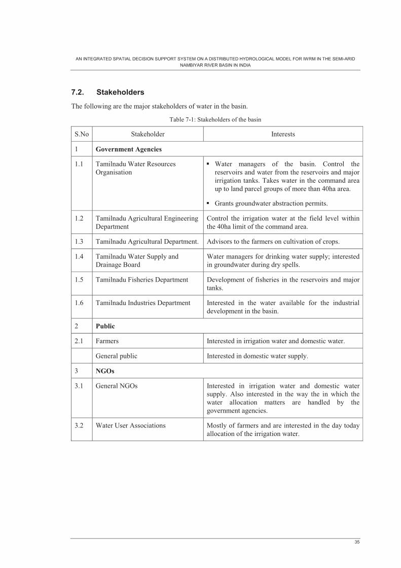
AN INTEGRATED SPATIAL DECISION SUPPORT SYSTEM ON A DISTRIBUTED HYDROLOGICAL MODEL FOR IWRM IN THE SEMI-ARID NAMBIYAR RIVER BASIN IN INDIA
35
7.2. Stakeholders
The following are the major stakeholders of water in the basin.
Table 7-1: Stakeholders of the basin
S.No Stakeholder Interests
1 Government Agencies
1.1 Tamilnadu Water Resources Organisation
� Water managers of the basin. Control the reservoirs and water from the reservoirs and major irrigation tanks. Takes water in the command area up to land parcel groups of more than 40ha area.
� Grants groundwater abstraction permits.
1.2 Tamilnadu Agricultural Engineering Department
Control the irrigation water at the field level within the 40ha limit of the command area.
1.3 Tamilnadu Agricultural Department. Advisors to the farmers on cultivation of crops.
1.4 Tamilnadu Water Supply and Drainage Board
Water managers for drinking water supply; interested in groundwater during dry spells.
1.5 Tamilnadu Fisheries Department Development of fisheries in the reservoirs and major tanks.
1.6 Tamilnadu Industries Department Interested in the water available for the industrial development in the basin.
2 Public
2.1 Farmers Interested in irrigation water and domestic water.
General public Interested in domestic water supply.
3 NGOs
3.1 General NGOs Interested in irrigation water and domestic water supply. Also interested in the way the in which the water allocation matters are handled by the government agencies.
3.2 Water User Associations Mostly of farmers and are interested in the day today allocation of the irrigation water.

AN INTEGRATED SPATIAL DECISION SUPPORT SYSTEM ON A DISTRIBUTED HYDROLOGICAL MODEL FOR IWRM IN THE SEMI-ARID NAMBIYAR RIVER BASIN IN INDIA
36
7.3. Conflicts
The prevailing major conflicts among the stakeholders in sharing the water resources are as below,
Table 7-2: Stakeholders and conflicts
S.No Water Stakeholders Complaints / Conflicts 1 Head-end farmers Vs. Tail-
end farmers. The Tail-end farmers grudge that the tail-end farmers do over irrigation to their crops and they are deprived of their share.
2 Water Managers Vs farmers
The water manages complain that the farmers are lavish in consuming more water by their age old irrigation practices and by always resorting to water intensive crops like paddy, sugarcane.
3 Water Supply Board Vs Basin Manager.
The basin manager allocates more water for irrigation rather than preserving it for drinking water supply.
4
Surface water
All Vs Basin Manager The water is wasted into the sea during wet years.
5 Basin Manager Vs Industrial consumers
The Basin Manager is restricting the groundwater abstraction permits.
6 Farmers & Water supply Board Vs Industrial consumers
The Industrial consumers are over exploiting the groundwater depriving the agriculture and drinking water needs.
7
Groundwater
Water Supply Board Vs Farmers and Industrial consumers
The farmers and industrial consumers deplete the scarce groundwater depriving the drinking water reserves.
This research aims to solve the above situation by concentrating on the item-5 as it is the only one situation regulated by the Basin manager by issuing abstraction permits.
7.4. Methodology
The following methodology is applied to solve the groundwater abstraction system.
1. Consider the basin as a single spatial unit. It hydrogeologically valid.
2. Input the abstraction rate of all the existing groundwater abstraction permit holders in the model.
3. Calculate the groundwater balance for a dry year.
4. Calculate the groundwater balance available spatially in the 61 villages of the basin.
5. Publish on the web the general availability of the groundwater balance in the villages along with the threshold limits decided by Collaborative Multicriteria Decision making as down below.

AN INTEGRATED SPATIAL DECISION SUPPORT SYSTEM ON A DISTRIBUTED HYDROLOGICAL MODEL FOR IWRM IN THE SEMI-ARID NAMBIYAR RIVER BASIN IN INDIA
37
6. This publication transparently informs in advance which villages are susceptible for any development involving groundwater abstraction.
7. When a request for the grant of a new groundwater abstraction permit is received by the Basin manager, he runs the model specifically to assess impact of the request.
8. If the simulated groundwater balance is above the pre-published threshold limit, the groundwater abstraction permit may be issued.
9. As a step on the positive side, the permit seeker may be encouraged to fund an Artificial Recharge Scheme. The hydrological model will predict the groundwater balance available in the scenario with the Artificial Recharge Scheme. This will improve the groundwater balance in the area and to that extent the grant of permit could be considered.
7.5. Collaborative Multi Criteria Decision Making
The collaborative multicriteria decision making is the solution to make a comprehensive decision in a socially acceptable manner. The following steps are involved in the process.
1) Generate alternative ways of using the groundwater during dry years. i.e. for Drinking, Agricultural and Industrial uses.
2) Prepare an allocation prioritising scale of 0 to 100%. The most importance is 100% and least importance is 0%. This scale is prepared based on multi criteria value table for each use as perceived by each shareholder.
Table 7-3: Value factors for Multi Criteria as per each shareholder
Value Factor for water Utility S.No Multi Criteria
Domestic Irrigation Industrial
1 Satisfying basic needs of people (0-100%)
2 Optimum use of a drop of water
3 Equitable sharing of water
4 Sustaining food production
5 Sustaining the ecology
6 Preventing sea water intrusion
7 Export of water to other basins
8 Employment opportunity
9 Economic prosperity of the people
10 Saving water for the future generation
Utility Factor, Ui (0-100%)

AN INTEGRATED SPATIAL DECISION SUPPORT SYSTEM ON A DISTRIBUTED HYDROLOGICAL MODEL FOR IWRM IN THE SEMI-ARID NAMBIYAR RIVER BASIN IN INDIA
38
3) Get the feedback of all the stake holders on prioritising the groundwater in the scale of prioritising.
4) Apply this Utility Factor for the groundwater abstraction, as below,
Pi,j = � (Ui x S x Q)/ 100000 Where, Pi,j = Prioritised quantity of groundwater abstraction for an Utility in a month. i = User (drinking, agriculture, industrial). J = Month of a dry year. Ui = Utility factor 0 – 100% to the demand as given by the Stakeholder. S = Stakeholder factor as assigned by the Basin manager. Q = Quantity of groundwater abstraction, m³/month. N = Number of stakeholders The ranking system is captured in the table below, for the basin.
Table 7-4: Prioritation of monthly water allocation
Domestic Irrigation Industrial S.No Stakeholder Stakeholder
factor, S
Qua
ntity
,Q, m
³
Util
ity
fact
or,
Ui
Qua
ntity
,Q ,
m³
Util
ity
fact
or,
Ui
Qua
ntity
,Q ,
m³
Util
ity
fact
or,
Ui
1 Tamilnadu Water Resources Organisation
90 600 100
2 Tamilnadu Agricultural Engineering Department
90
3 Tamilnadu Agricultural Department.
90
4 Tamilnadu Water Supply and Drainage Board
90
5 Tamilnadu Fisheries Department
80
6 Tamilnadu Industries Department
90
7 Representative of farmers 90
8 Representative of public 90
9 NGOs 50
10 Water User Associations 90
11 University 60
12 District Administrator 90
Abstraction /month 1000
5) Thus the temporal distribution of groundwater allocation among the three uses of Domestic, Agricultural and Industrial purposes in the basin are prefixed in a collaborative way.
These prioritised quantities are the thresholds for the groundwater abstraction in the hydrological model

AN INTEGRATED SPATIAL DECISION SUPPORT SYSTEM ON A DISTRIBUTED HYDROLOGICAL MODEL FOR IWRM IN THE SEMI-ARID NAMBIYAR RIVER BASIN IN INDIA
39
8. Results
8.1. General
The model has limited calibration and an average correlation coefficient of 0.32 only is achieved. The model needs more detailed calibration with field tests to derive any discerning results of quantitative results. However the analysis of the model output as it is still yields the following findings in the pattern of behaviour of the basin.
8.2. Saturated Zone storage
The saturated zone storage responds well in consonance with the rainfall events. It implies that the actual overland infiltration and the recharge to the groundwater table are fairly good. Still the groundwater table is much below the ground level. Hence there is high potential for constructing more artificial recharge structures in the basin.
8.3. Evapotranspiration
It is seen from the water balance of the basin that a substantial potion of the rainfall goes back as evapotranspiration, even in the non agricultural years. These evapotranspiration is originates from the baresoil having patchy grass and bushes. Hence the ideal way of preserving the rainwater is to take into the groundwater table
8.4. Base flow into the river
The following two sets of auto calibration of the model were run between the following observed and simulated state variables.
a) 11 Piezometric heads only and
b) 11 Piezometric heads and river discharge at outlet.
Both these runs yields the same autocalibrated values for the soil parameters like hydraulic conductivities and specific yield. It implies that these soil parameters and the river discharge are not correlated. It means that there is no base flow into the river from the saturated zone and the river is a loosing river. Hence the river is also a fit place to construct artificial recharge structures.
8.5. Research objectives
The objectives of the research are met and the research questions are answered as follows,
8.5.1. Dynamic local scale assessment of water
The research succeeded in developing a method for the dynamic and local scale assessment of the water in the basin as follows,
a) A 3 Dimentional distributed fully transient model to represent the basin is developed. b) The extensive network of irrigation system is captured in the model. The main river is
captured in the model. Only the channel system has to be included which is a labour intensive assignment by itself.

AN INTEGRATED SPATIAL DECISION SUPPORT SYSTEM ON A DISTRIBUTED HYDROLOGICAL MODEL FOR IWRM IN THE SEMI-ARID NAMBIYAR RIVER BASIN IN INDIA
40
c) Dynamic assessment of the groundwater, even on every day basis at any location within the basin is make feasible through this model.
d) With further calibration the model will yield more refined and quantitatively accurate results.
The research succeeded in developing a method for the dynamic and local scale assessment of the water in the basin as follows,
8.5.2. Framework for water allocation
The research succeeded in developing a water allocation framework through Collaborative Multi Criteria Decision Making. The research has decisively come up with a specific methodology for the intricate subject of grant of groundwater abstraction permits. This methodology is scientifically sound based on a numerical model. It is also socially acceptable as it is based on Collaborative Multi Criteria Decision Making taking all the stakeholders in to confidence.
8.6. Further works to be done
This research succeeded in finding a water allocation framework built on a hydrological model and Collaborative Multi Criteria Decision Making. This model needs further improvements to get more refined outputs
1. Field tests should be conducted to assess the soil parameters and the model be calibrated and validated further.
2. The drainage system interconnecting the river and the irrigation tanks should be included in the model.
3. The impact of the conductance values in the bed material of the irrigation tanks.

AN INTEGRATED SPATIAL DECISION SUPPORT SYSTEM ON A DISTRIBUTED HYDROLOGICAL MODEL FOR IWRM IN THE SEMI-ARID NAMBIYAR RIVER BASIN IN INDIA
41
9. Executive summary
The following water allocation framework may be adopted for granting groundwater abstraction permits in the basin as a pilot scheme and extended to the other 33 river basins in the state in future.
1) The general groundwater balance in each village in the basin, based on the assessment with the basin as a single hydrogeological unit, may be published on the government website as general prior information. It informs the groundwater abstraction permit seekers in advance, of the prospects of getting the grant of permit and helps them pre-plan the location of their facilities.
2) The actual grant of groundwater abstraction permits could be made for each individual case by applying the request in this model. If the request’s impact on the groundwater balance is above the predefined threshold derived by Collaborative Multi Criteria Decision making of the stakeholders, the permit could be granted.
3) The water abstraction permit seekers may be encouraged to fund/ part fund the artificial recharge schemes in the basin. They may be granted water abstraction permits proportionate to the additional groundwater recharged by these schemes


AN INTEGRATED SPATIAL DECISION SUPPORT SYSTEM ON A DISTRIBUTED HYDROLOGICAL MODEL FOR IWRM IN THE SEMI-ARID NAMBIYAR RIVER BASIN IN INDIA
43
10. References
Becu, N., Neef, A., Schreinemachers, P. and Sangkapitux, C., 2008. Participatory computer simulation to support collective decision-making: Potential and limits of stakeholder involvement. Land Use Policy, 25(4): 498-509.
Henriksen, H.J., Troldborg, L., Højberg, A.L. and Refsgaard, J.C., 2008. Assessment of exploitable groundwater resources of Denmark by use of ensemble resource indicators and a numerical groundwater-surface water model. Journal of Hydrology, 348(1-2): 224-240.
Henriksen, H.J. et al., 2003. Methodology for construction, calibration and validation of a national hydrological model for Denmark. Journal of Hydrology, 280(1-4): 52-71.
Kluge, T. et al., 2008. IWRM concept for the Cuvelai Basin in northern Namibia. Physics and Chemistry of the Earth, Parts A/B/C, 33(1-2): 48-55.
Maneta, M., Schnabel, S. and Jetten, V., 2008. Continuous spatially distributed simulation of surface and subsurface hydrological processes in a small semiarid catchment. Hydrological Processes, 22(13): 2196-2214.
Stisen, S., Jensen, K.H., Sandholt, I. and Grimes, D.I.F., 2008. A remote sensing driven distributed hydrological model of the Senegal River basin. Journal of Hydrology, 354(1-4): 131-148.

44
11. Appendix
11.1. Typical Water Balance of the basin

AN INTEGRATED SPATIAL DECISION SUPPORT SYSTEM ON A DISTRIBUTED HYDROLOGICAL MODEL FOR IWRM IN THE SEMI-ARID NAMBIYAR RIVER BASIN IN INDIA
45
11.2. FAO Penman-Motieth Method of calculating ETo.
FAO Penman-Monteith method equation is given as:
)34.01(
)(273
900)(408.0
2
2
0 u
eeuT
GRET
asn
++Δ
−+
+−=
γ
γ
Where: ET0 = reference evapotranspiration [mm day-1] Rn = net radiation [MJ m-2 day-1] G = soil heat flux density [MJ m-2 day-1] T = air temperature at 2 m height [0C] u2 = wind speed at 2 m height [m s-1] � = slope vapour pressure curve [kPa 0C-1] � = psychometric constant [kPa 0C-1] es & ea = saturation and actual vapour pressure respectively [kpa]

46
11.3. Visuals of Irrigation Tank, Weir, Command area
The following visuals are for the better comprehension of the system of Irrigation Tanks and Irrigation Wells in the Nambiyar river basin in India.
Irrigation Tank Command Area under Irrigation Tank
Weir Command area under Irrigation Well
Command Area and Irrigation Tank Bare soil