An Intelligent Portable Aerial Surveillance System:Modeling and Image Stitching

by

Ruixiang Du

A ThesisSubmitted to the Faculty

of theWORCESTER POLYTECHNIC INSTITUTE

in partial fulfillment of the requirements for theDegree of Master of Science

in

Robotics Engineeringby

MAY 2013

APPROVED:

Professor Taskin Padir, Advisor

Professor Michael A. Gennert, Committee Member

Professor Xinming Huang, Committee Member

Abstract

Unmanned Aerial Vehicles (UAVs) have been widely used in modern warfare for surveil-

lance, reconnaissance and even attack missions. They can provide valuable battlefield in-

formation and accomplish dangerous tasks with minimal risk of loss of lives and personal

injuries. However, existing UAV systems are far from perfect to meet all possible situations.

One of the most notable situations is the support for individual troops. Besides the incapa-

bility to always provide images in desired resolution, currently available systems are either

too expensive for large-scale deployment or too heavy and complex for a single solder. In-

telligent Portable Aerial Surveillance System (IPASS), sponsored by the Air Force Research

Laboratory (AFRL), is aimed at developing a low-cost, light-weight unmanned aerial vehicle

that can provide sufficient battlefield intelligence for individual troops. The main contri-

butions of this thesis are two-fold (1) the development and verification of a model-based

flight simulation for the aircraft, (2) comparison of image stitching techniques to provide

a comprehensive aerial surveillance information from multiple vision. To assist with the

design and control of the aircraft, dynamical models are established at different complexity

levels. Simulations with these models are implemented in Matlab to study the dynamical

characteristics of the aircraft. Aerial images acquired from the three onboard cameras are

processed after getting the flying platform built. How a particular image is formed from

a camera and the general pipeline of the feature-based image stitching method are first

introduced in the thesis. To better satisfy the needs of this application, a homography-

based stitching method is studied. This method can greatly reduce computation time with

very little compromise in the quality of the panorama, which makes real-time video display

of the surroundings on the ground station possible. By implementing both of the meth-

ods for image stitching using OpenCV, a quantitative comparison in the performance is

accomplished.

iii

Acknowledgements

I would like to express my deepest appreciation to all those who provided me the pos-

sibility to complete this thesis.

To start I would like to thank my advisor Professor Taskin Padir. Without his great

patience, valuable guidance and persistent help, I would never have been able to finish this

project and learn so much in this process. I consider it an honor to work with him in his

Robotics and Intelligent Vehicles Research Laboratory.

I would like to thank my committee members, Professor Michael A. Gennert and Pro-

fessor Xinming Huang, for their insightful comments and suggestions.

I would also like to thank the IPASS team, Adam Blumenau, Alec Ishak, Brett Limone,

Zachary Mintz, Corey Russell and Adrian Sudol. Their works for the IPASS project made

it possible for me to test and verify part of my research. Our discussion and idea exchanging

inspired me a lot to delve further into this project.

Further more, I would like to thank my friends, Gang Li and Xianchao Long. They

provided kindly help when I got in trouble during my works.

Finally, I would like to thank my parents, Xintian Du and Wenxia Yu. Without their

support, I would never have a chance to study at Worcester Polytechnic Institute in the

United States. Their selfless love and encouragement always keeps me moving forward in

my life and career.

iv

Contents

List of Figures vi

List of Tables viii

1 Introduction 11.1 Background . . . . . . . . . . . . . . . . . . . . . . . . . . . . . . . . . . . . 1

1.1.1 WASP III . . . . . . . . . . . . . . . . . . . . . . . . . . . . . . . . . 31.1.2 RQ-11 Raven . . . . . . . . . . . . . . . . . . . . . . . . . . . . . . . 31.1.3 RQ-16 T-Hawk . . . . . . . . . . . . . . . . . . . . . . . . . . . . . . 5

1.2 Objectives of the IPASS Project . . . . . . . . . . . . . . . . . . . . . . . . 61.2.1 Needs Analysis . . . . . . . . . . . . . . . . . . . . . . . . . . . . . . 61.2.2 System Requirements . . . . . . . . . . . . . . . . . . . . . . . . . . 6

1.3 Thesis Contributions . . . . . . . . . . . . . . . . . . . . . . . . . . . . . . . 71.4 Literature Review . . . . . . . . . . . . . . . . . . . . . . . . . . . . . . . . 81.5 Thesis Organization . . . . . . . . . . . . . . . . . . . . . . . . . . . . . . . 9

2 System Design of IPASS 112.1 Mechanical Design . . . . . . . . . . . . . . . . . . . . . . . . . . . . . . . . 112.2 Electronic Design . . . . . . . . . . . . . . . . . . . . . . . . . . . . . . . . . 132.3 Software Design . . . . . . . . . . . . . . . . . . . . . . . . . . . . . . . . . . 15

2.3.1 Embedded Software . . . . . . . . . . . . . . . . . . . . . . . . . . . 152.3.2 Software for Ground Station . . . . . . . . . . . . . . . . . . . . . . 16

2.4 Final Product of the IPASS Project . . . . . . . . . . . . . . . . . . . . . . 172.5 Chapter Conclusion . . . . . . . . . . . . . . . . . . . . . . . . . . . . . . . 17

3 Modeling and Simulation 193.1 Modeling . . . . . . . . . . . . . . . . . . . . . . . . . . . . . . . . . . . . . 19

3.1.1 Basic Model . . . . . . . . . . . . . . . . . . . . . . . . . . . . . . . . 193.1.2 2D Model . . . . . . . . . . . . . . . . . . . . . . . . . . . . . . . . . 203.1.3 3D Model . . . . . . . . . . . . . . . . . . . . . . . . . . . . . . . . . 22

3.2 Matlab Simulation . . . . . . . . . . . . . . . . . . . . . . . . . . . . . . . . 243.2.1 Simulation Process . . . . . . . . . . . . . . . . . . . . . . . . . . . . 243.2.2 3D Animation for the Simulation . . . . . . . . . . . . . . . . . . . . 25

v

3.2.3 Simulation with the Basic Model . . . . . . . . . . . . . . . . . . . . 273.2.4 Simulation with the 2D Model . . . . . . . . . . . . . . . . . . . . . 283.2.5 Simulation with the 3D Model . . . . . . . . . . . . . . . . . . . . . 30

3.3 Chapter Conclusion . . . . . . . . . . . . . . . . . . . . . . . . . . . . . . . 33

4 Image Stitching 354.1 Image Formation . . . . . . . . . . . . . . . . . . . . . . . . . . . . . . . . . 354.2 Motion Models . . . . . . . . . . . . . . . . . . . . . . . . . . . . . . . . . . 384.3 Feature-based Image Stitching . . . . . . . . . . . . . . . . . . . . . . . . . 39

4.3.1 Feature-based Registration . . . . . . . . . . . . . . . . . . . . . . . 404.3.2 Compositing . . . . . . . . . . . . . . . . . . . . . . . . . . . . . . . 44

4.4 Homography Based Stitching . . . . . . . . . . . . . . . . . . . . . . . . . . 454.4.1 Homography . . . . . . . . . . . . . . . . . . . . . . . . . . . . . . . 464.4.2 Plane induced parallax . . . . . . . . . . . . . . . . . . . . . . . . . . 474.4.3 Infinite Homography . . . . . . . . . . . . . . . . . . . . . . . . . . . 494.4.4 Camera Calibration . . . . . . . . . . . . . . . . . . . . . . . . . . . 52

4.5 Comparison of the Two Image Stitching Methods . . . . . . . . . . . . . . . 55

5 Conclusion and Future Work 61

Bibliography 63

A Appendix A: Matlab Simulation Code for the 3D Model 65A.1 simulation.m . . . . . . . . . . . . . . . . . . . . . . . . . . . . . . . . . . . 65A.2 ipass.m . . . . . . . . . . . . . . . . . . . . . . . . . . . . . . . . . . . . . . 70

B Appendix B: C++ Code for Homography-based Image Stitching Method 74B.1 homostitch.h . . . . . . . . . . . . . . . . . . . . . . . . . . . . . . . . . . . 74B.2 homostitch.cpp . . . . . . . . . . . . . . . . . . . . . . . . . . . . . . . . . . 75

vi

List of Figures

1.1 WASP III [1] . . . . . . . . . . . . . . . . . . . . . . . . . . . . . . . . . . . 21.2 RQ-11 Raven [2] . . . . . . . . . . . . . . . . . . . . . . . . . . . . . . . . . 31.3 RQ16 T-Hawk [3] . . . . . . . . . . . . . . . . . . . . . . . . . . . . . . . . . 5

2.1 Two Prototypes of the Chassis . . . . . . . . . . . . . . . . . . . . . . . . . 122.2 Final Design of the Chassis . . . . . . . . . . . . . . . . . . . . . . . . . . . 132.3 Electronic Box and Cameras . . . . . . . . . . . . . . . . . . . . . . . . . . . 142.4 System Diagram of the System . . . . . . . . . . . . . . . . . . . . . . . . . 152.5 Ground Station Software Developed by IPASS Team . . . . . . . . . . . . . 162.6 The Whole Intelligent Portable Aerial Surveillance System . . . . . . . . . 172.7 Image Stitching Result by IPASS team . . . . . . . . . . . . . . . . . . . . . 18

3.1 Force and Moment Analysis of the Basic Model . . . . . . . . . . . . . . . . 193.2 Force and Moment Analysis of the 2D Model . . . . . . . . . . . . . . . . . 213.3 Coordinate System of the 3D Model . . . . . . . . . . . . . . . . . . . . . . 223.4 Mechanical Model of the Aircraft in Sketchup . . . . . . . . . . . . . . . . . 263.5 Virtual Reality Scene in vrbuild2 . . . . . . . . . . . . . . . . . . . . . . . . 263.6 PD Control: desired value z=10, psi=0.785 (45 degrees) . . . . . . . . . . . 273.7 Simulation with Basic Model . . . . . . . . . . . . . . . . . . . . . . . . . . 273.8 Simulation with 2D Model . . . . . . . . . . . . . . . . . . . . . . . . . . . . 283.9 Flight Trajectory with Different values of the Offset e . . . . . . . . . . . . 293.10 Simulation of the Aircraft with Only Rotation about Center Axis . . . . . . 303.11 Simulation of the Aircraft with Only Offset of the Mass Center . . . . . . . 313.12 Simulation of the Aircraft when τ = 0.15 and e=0.01m . . . . . . . . . . . . 323.13 Simulation of the Aircraft when τ = 0.35 and e=0.01m . . . . . . . . . . . . 333.14 Flight Test . . . . . . . . . . . . . . . . . . . . . . . . . . . . . . . . . . . . 34

4.1 Pinhole Camera Model . . . . . . . . . . . . . . . . . . . . . . . . . . . . . . 364.2 Four Coordinates in the Image Formation . . . . . . . . . . . . . . . . . . . 374.3 Basic set of 2D planar transformations [4] . . . . . . . . . . . . . . . . . . . 384.4 Hierarchy of 2D coordinate transformations [4] . . . . . . . . . . . . . . . . 394.5 Pipeline of Feature-based Stitching Method from OpenCV Library . . . . . 404.6 Test Frame with Two Microsoft Webcams . . . . . . . . . . . . . . . . . . . 41

vii

4.7 Original Images Taken by the Two Cameras . . . . . . . . . . . . . . . . . . 424.8 SURF Feature Points in the Two Images . . . . . . . . . . . . . . . . . . . . 434.9 Matching of SURF Feature Points . . . . . . . . . . . . . . . . . . . . . . . 444.10 Stitching Result with a Planar Compositing Surface . . . . . . . . . . . . . 454.11 Stitching Result with a Spherical Compositing Surface . . . . . . . . . . . . 464.12 Homography between Two Image Planes [5] . . . . . . . . . . . . . . . . . . 474.13 Transformations of Three Cameras with Homography . . . . . . . . . . . . 484.14 Chessboard with Corners Marked by Color Circles and Lines . . . . . . . . 494.15 Image Alignment using Homography (without misalignment) . . . . . . . . 504.16 Image Alignment using Homography (with misalignment) . . . . . . . . . . 514.17 Distortion of a Camera: (a) No Distortion (b)Barrel Distortion (c) Pincush-

ion Distortion [6] . . . . . . . . . . . . . . . . . . . . . . . . . . . . . . . . . 534.18 Distortion Correction: (Left) distorted image (Right) undistorted image . . 544.19 Image Alignment with Infinite Homography . . . . . . . . . . . . . . . . . . 564.20 Simplified Pipelines of Feature-based Method and Homography-based Method 574.21 GUI of the Application for Image Stitching . . . . . . . . . . . . . . . . . . 584.22 Comparison of Panoramas - top: feature-based method, bottom: homography-

based method . . . . . . . . . . . . . . . . . . . . . . . . . . . . . . . . . . . 59

viii

List of Tables

1.1 General Characteristics of WASP III [1] . . . . . . . . . . . . . . . . . . . . 21.2 General Characteristics of RQ-11 Raven [2] . . . . . . . . . . . . . . . . . . 41.3 General Characteristics of RQ-16 T-Hawk (adapted from [3], [7] and [8]) . . 4

2.1 List of Components . . . . . . . . . . . . . . . . . . . . . . . . . . . . . . . . 14

4.1 Update Frequency of the Two Stitching Methods . . . . . . . . . . . . . . . 58

1

Chapter 1

Introduction

1.1 Background

Unmanned Aerial Vehicles (UAVs) have been widely used in a variety of areas in modern

world since their first appearance in early nineties. With the help of the achievements in

technology fields such as automatic control, autonomous navigation and communication,

now UAVs can accomplish various kinds of tasks that once required a human pilot to do

onboard. Since the use of UAVs eliminates the possibilities of loss of lives and personal

injuries, UAVs are especially suitable for tasks that need to be performed in dangerous

environments.

Currently, UAVs are deployed predominantly for military applications. They are mostly

used for reconnaissance to provide battle field intelligence and the attack to objects in special

areas. This thesis focuses on the UAVs that are designed for reconnaissance missions. A

large number of models for this purpose have been developed so far. These models are

classified by different standards, such as scale and flight time. Since the research has a

concentration on small scale UAVs for reconnaissance, several such existing models are

briefly introduced below.

2

Figure 1.1: WASP III [1]

Primary function Reconnaissance and surveillance with low-altitude operation

Contractor Aerovironment, Inc. (Increment III)

Power plant Electric motor, rechargeable lithium ion batteries

Wingspan 28.5 inches (72.3 cm)

Length 10 inches (25.4 cm)

Weight (air vehicle) 1 pound (453 grams)

Weight (total system) 14.4 pounds (6.53 kilograms)

Speed 20 - 40 mph

Operating altitude From 150 to 500+ feet above ground level (to 152+ meters)

Altitude 1,000 feet

System Cost approximately $49,000 (2006 dollars)

Payload High resolution, day/night camera

Table 1.1: General Characteristics of WASP III [1]

3

1.1.1 WASP III

According to [1], “the Air Force’s Wasp III small unmanned aircraft system provides real-

time direct situational awareness and target information for Air Force Special Operations

Command Battlefield Airmen.” This system mainly consists of three parts: the expendable

air vehicle, a ground control unit and communications ground station. It can either be

controlled by one operator with a handheld control unit or perform tasks fully autonomously

from takeoff to recovery. General characteristics of WASP III are shown in Table 1.1.

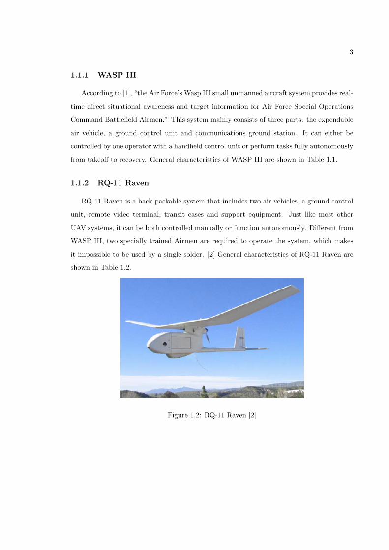
1.1.2 RQ-11 Raven

RQ-11 Raven is a back-packable system that includes two air vehicles, a ground control

unit, remote video terminal, transit cases and support equipment. Just like most other

UAV systems, it can be both controlled manually or function autonomously. Different from

WASP III, two specially trained Airmen are required to operate the system, which makes

it impossible to be used by a single solder. [2] General characteristics of RQ-11 Raven are

shown in Table 1.2.

Figure 1.2: RQ-11 Raven [2]

4

Primary function Reconnaissance and surveillance with low-altitude operation

Contractor Aerovironment, Inc.

Power plant Electric Motor, rechargeable lithium ion batteries

Wingspan 4.5 feet (1.37 meters)

Weight 4.2 lbs (1.9 kilograms)

Weight(ground control unit) 17 lbs (7.7 kilograms)

Speed 30-60 mph (26-52 knots)

Range 8-12 km (4.9-7.45 miles)

Endurance 60-90 minutes

Altitude (operations) 100-500 feet air ground level ( to 152 meters)

System Cost approximately $173,000 (2004 dollars)

Payload High resolution, day/night camera and thermal imager

Table 1.2: General Characteristics of RQ-11 Raven [2]

Primary function Surveillance

Contractor Honeywell

Power plant 1 3W-56 56cc Boxer Twin piston engine, 4 hp (3 kW) each

Gross Weight 20 lb (8.4 kg)

Rate of Climb 4.2 lbs (1.9 kilograms)

Speed 46 mph

Range 3-6 mile (5-10km)

Service ceiling 10,000 ft (3,048 m)

Endurance 50 min

System Cost $450,000

Payload one forward and one downward looking daylight or IR cameras

Table 1.3: General Characteristics of RQ-16 T-Hawk (adapted from [3], [7] and [8])

5

Figure 1.3: RQ16 T-Hawk [3]

1.1.3 RQ-16 T-Hawk

Developed by Honeywell, RQ-16 T-Hawk is a ducted fan micro UAV, which is capable

of vertical take-off and landing (VTOL). It has been used in Iraq to search for roadside

bombs since 2007. And the great success in Iraq has attracted more orders from the U.S.

Navy. “On September 19, 2012, Honeywell was awarded a support contract for the RQ-16B

Block II T-Hawk for its continued service.” [3] General characteristics of RQ-16 T-Hawk

are shown in Table 1.3.

Though these models have excellent performance and their capabilities have been proven

in battlefield, they’re still far from perfect to satisfy all real-world situations. One of the

most noticeable situations is that these systems are not suitable enough to meet the needs

of individual troops. None of them can be carried and operated by a single soldier while

this soldier still has other tasks to do. Moreover, the prices for these unmanned aerial

vehicle systems are too high to make it realistic for widely deployment. Thus a new type

of low-cost, light weight aerial surveillance equipment is still desired.

Intelligent Portable Aerial Surveillance System (IPASS), sponsored by the Air Force

6

Research Laboratory (AFRL), is aimed at developing such a system that can be used by

US Ground Forces. It’s supposed to be used by individual soldiers and be capable of

providing sufficient battlefield information with a low system cost.

1.2 Objectives of the IPASS Project

1.2.1 Needs Analysis

This project aims at small scale aircraft that can be easily carried, deployed and operated

by a single soldier. The desired aircraft needs to be capable of lifting off rapidly to a height

of over 100 feet, streaming 360 degree high-resolution color video in real-time to a ground

station and finally landing to the ground safely. The ground station needs to be able to

receive data from the aircraft, display images in real-time and allow the user to check

interest points on the images. Moreover, the whole system should not be too expensive so

that it can be widely equipped by soldiers.

1.2.2 System Requirements

To satisfy the needs of the US Ground Forces for this kind of portable aerial surveillance

system, some design requirements are defined below. These requirements are used for the

design and evaluation of the new system. They are stated separately for the aircraft and

the ground station as follows [9]:

For the aircraft:

• The aircraft must be lighter than 10kg.

• The aircraft must be able to lift off and reach a height of at least 30 meters.

• The aircraft must have vision system onboard and provide a 360-degree view of the

surrounding area while in the air.

• The aircraft must be able to get its position coordinate.

• The system must be able to transmit wireless to a ground station with a downlink

rage of up to 200 m.

7

• The aircraft must be able to survive from a fall of 10 meters with all electronic

components functioning normally.

For the ground station:

• The ground station must be able to communicate with the aircraft and stream video

in real-time.

• The ground station must be able to stitch images to generate 360-degree view panora-

mas

• The ground station must be able to display images and location information of the

aircraft.

• The ground station must provide a GUI that allows a normal soldier to understand

and operate proficiently after 1-hour training.

1.3 Thesis Contributions

The IPASS team, which consists of six undergraduate students of WPI, did all the system

integration works of the IPASS project as their MQP (Major Qualifying Project). They

designed and manufactured the mechanical structure of the aircraft, chose and integrate

modular circuit boards and wrote code of low level functions for the two processors onboard.

They also implemented a ground station software with basic functions for image stitching.

The research first aims at helping the IPASS team to meet the requirements of the

IPASS project, but it is extended to solve for more general problems of mobile robots that

are required to perform similar tasks. Achievements of the research can provide theoretical

supports to the IPASS project directly. Moreover, documents and codes developed along

with the research can be adapted for similar future projects, which are valuable resources

to save time and money.

This thesis mainly works on two aspects. (1) The first is the modeling and simulation

of the aircraft. This part of work is to develop the kinematics and dynamics models of the

aircraft designed by the IPASS team. These models can reveal how the aircraft behaves

8

under the drive of specific system inputs mathematically. It’s a fundamental step for the

design of flight control algorithms. Simulation with these models is performed under Matlab,

which can help to find physical characteristics of the aircraft and improve the design before

the real one is ready for testing. (2) The other part of work for the thesis is the discussion of

two methods of image stitching. The popular feature-based method is explained first. This

method has drawn great interests from researchers in the field of computer science in recent

years but less attention was ever paid to its application on mobile robots. Furthermore, to

better satisfy the needs of image stitching for the purpose of surveillance, a homography-

based method is studied. With the use of OpenCV, both of these stitching methods are

implemented and the stitching results are compared. Advantages and disadvantages of each

method are concluded. These conclusions can help people to choose the right method for

different situations of image stitching.

1.4 Literature Review

The aircraft developed by IPASS team has a novel structure, but its kinematics and

dynamics are very similar to those of a Quadrotor. Since there are a lot of papers studying

the modeling and simulation of a Quadrotor, these resources can be very useful in the

modeling work for IPASS. [10] is a technical report that gives a step-by-step illustration of

how a dynamic model of a Quadrotor is developed. It also presents a controller design that

can be used for the attitude control of the Quadrotor. [11] presents the modeling process

using the Newton-Euler method. It also discusses the dynamics of brushless motors used

in the aircraft. Besides giving a similar model with that in [11], [12] further introduces

an automatic stabilization system for quadrotors with applications to vertical take-off and

landing. Chapter 3 of [13] introduces the modeling of a Quadrotor using the Euler-Lagrange

method. All these literatures contribute a lot in the derivation of the 3D model of the aircraft

in IPASS.

Image stitching has been widely used in many applications in recent years. [4] intro-

duces the basics of computer vision including how an image is formed from a camera,

motion models and common image processing methods. [14] gives an outline of the im-

9

age stitching techniques. It presented a simplified flowchart of producing panoramic image

from image acquisition to image remapping and finally to image blending. [15] introduces

the automatic panoramic image stitching method using invariant features. It provides de-

tailed algorithm descriptions about how images can be automatically stitched using SIFT

features and RANSAC homography estimation. [16] makes though illustration of feature-

based image stitching. Theories about feature extraction, feature matching, homography

estimation, image wrapping and image blending are all introduced in this material. [5]

makes comprehensive illustration of two-view geometry. The concept of homography and

infinite homography are explained in this book. To implement the homography-based stitch-

ing method, camera calibration is used. [4] and [17] introduces single camera calibration

and stereo calibration from theories to practice. [18] is a tutorial for the use of OpenCV

library. It presents what functions are provided by the library and how these functions can

be used to implement camera calibration and image stitching algorithms.

1.5 Thesis Organization

Chapter 1 presents the background of the thesis. Several existing UAV systems are in-

troduced concisely, which brings the motivation for the IPASS project. Then the objectives

of the IPASS project are stated. This part includes the needs analysis and the definition of

system requirements. Afterwards, thesis contributions are summarized. Literature review

part lists some relative materials that have made notable progress in the areas that this

thesis works on. Literatures about the modeling of a quadrotor and image stitching are

introduced respectively.

Chapter 2 briefly introduces the system design of the aircraft system developed by the

IPASS team. This chapter includes the mechanical design, electronic design and software

design of the IPASS system. Since the research topics of the thesis originate from this

project, these introductions can be very helpful to understand what the problems are and

how the research can help to better meet the application requirements.

Chapter 3 presents the modeling and simulation of the aircraft. The model is developed

from three different complexity levels. An ideal model is first introduced to illustrate the

10

basic characteristics of the aircraft design. Then this model is further extended to a 2D

model, which aims at studying the influence to the flight trajectory introduced by the

offset of mass center. Finally a fully 3D model is completed, which can reflect the overall

performance of the aircraft during the flight with the consideration of both offset of mass

center and self-rotation. All three models are simulated in Matlab and the simulation results

are compared with the actual flight of the aircraft.

Chapter 4 demonstrates two methods of image stitching that are used for this applica-

tion. The feature-based image stitching method is briefly introduced first. This method

uses matched feature points to estimate the relative position and orientation of image pairs

for the stitching. To improve the stitching speed, the homography-based stitching method

is studied. The concept of infinite homography is brought out to solve the problem of im-

age alignment. To realize this optimized method for mobile robots, camera calibration is

also introduced in this chapter. The last part of this chapter makes comparison between

these two image stitching methods. Both advantages and disadvantages of each method are

discussed.

Chapter 5 concludes the main contents of this thesis. This chapter also states some

known defects of the current system and some possible future works are proposed.

11

Chapter 2

System Design of IPASS

IPASS is designed for individual troops. To minimize the distraction from the soldier

that may be caused by the system, the aircraft is designed to be autonomous and its

operation is expected to be as simple as possible. It is required that the aircraft can lift off

to a specific height in a short time and land to the ground automatically after it takes photos

of the battlefield around the peak of its flight trajectory. Through the entire process, it’s

desired that the soldier only need to press the start button, receive photos of the battlefield

and then take back the landed aircraft.To fulfill these requirements for the system, special

attentions are paid on both of the hardware and software design.

2.1 Mechanical Design

The mechanical structure of the aircraft mainly consists of two parts, the chassis and

the electronic box. All circuit boards are placed in the electronic box, which protects these

boards from damages. As shown in Figure 2.1, several prototypes were built before the

final design was determined. With experiments on these prototypes, two primary problems

get solved: the structural strength of the whole aircraft and the capability of the chassis to

protect propellers. As defined in the requirements of the system, the aircraft should be able

to survive from 10-meter fall intact. Thus the structural strength must be guaranteed as a

main concern. From actual flight tests, it’s found that the propellers are very easy to be

severely damaged when the aircraft falls to the ground with the propellers rotating at a very

12

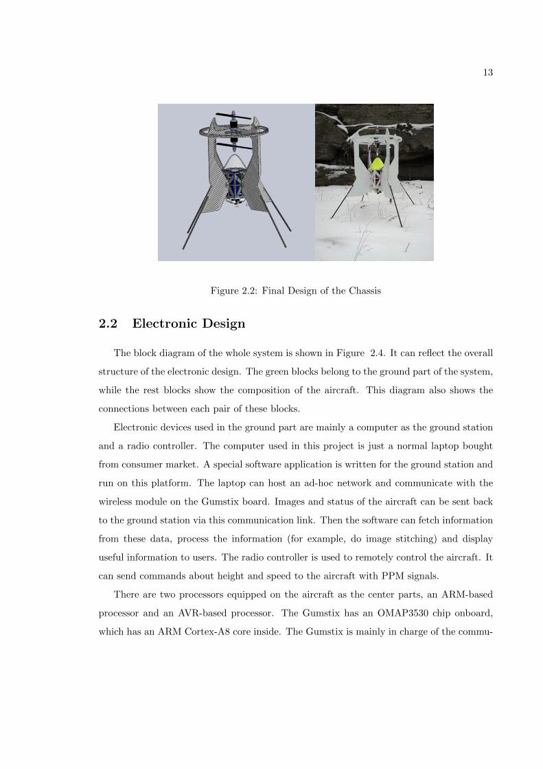
high speed. To avoid such occasions, the structure around the propellers were redesigned.

The final design of the chassis (shown in Figure 2.2) can hold both of the propulsion system

and the electronic box stably and it also provides protection of the propellers from possible

collisions when the aircraft fails to the ground. At the bottom of the electronic box, three

holes are designed with a specific angle between each other (shown in Figure 2.3). These

three holes are used to hold the cameras so that three images from different view angles

can be taken at the same time and further used to compose a 360-degree panorama.

Figure 2.1: Two Prototypes of the Chassis

The body part of the chassis is made of Coroplast, a kind of polypropylene copolymer.

This type of material is very lightweight and its special crumpling structure makes it capa-

ble of absorbing impacts from collision to save other more valuable electronic parts. The

electronic box is manufactured by a 3D printer and the material used is ABS plastic. Both

of these two kinds of materials for the mechanical structure are low-cost and have desired

physical characteristics. Thus they can fulfill the requirements for the mechanical design as

described above.

13

Figure 2.2: Final Design of the Chassis

2.2 Electronic Design

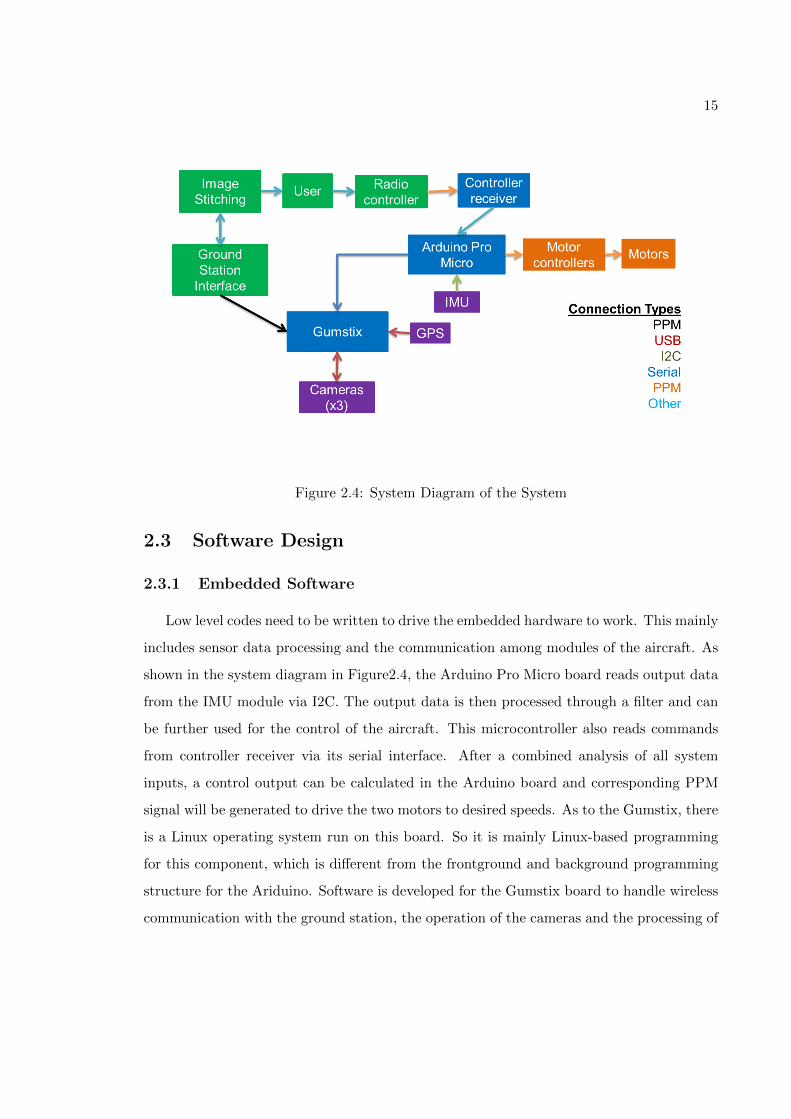
The block diagram of the whole system is shown in Figure 2.4. It can reflect the overall

structure of the electronic design. The green blocks belong to the ground part of the system,

while the rest blocks show the composition of the aircraft. This diagram also shows the

connections between each pair of these blocks.

Electronic devices used in the ground part are mainly a computer as the ground station

and a radio controller. The computer used in this project is just a normal laptop bought

from consumer market. A special software application is written for the ground station and

run on this platform. The laptop can host an ad-hoc network and communicate with the

wireless module on the Gumstix board. Images and status of the aircraft can be sent back

to the ground station via this communication link. Then the software can fetch information

from these data, process the information (for example, do image stitching) and display

useful information to users. The radio controller is used to remotely control the aircraft. It

can send commands about height and speed to the aircraft with PPM signals.

There are two processors equipped on the aircraft as the center parts, an ARM-based

processor and an AVR-based processor. The Gumstix has an OMAP3530 chip onboard,

which has an ARM Cortex-A8 core inside. The Gumstix is mainly in charge of the commu-

14

Figure 2.3: Electronic Box and Cameras

Item Model Number

Ground Station Laptop Lenovo Thinkpad W530 1

Gumstix Overo FE COM 1

Arduino Micro Pro 1

Camera SB101C USB Camera 3

IMU RoBoard 9 DOF IMU 1

GPS ND-100S Globalsat USB 1

Table 2.1: List of Components

nications. It collects images from the cameras and then sends the images back to the ground

station via its wireless module. Additionally, it also deals with data from the GPS module.

The Arduino Pro Micro board includes an ATMega 32U4 microcontroller. This Arduino

board is mainly used to perform low level functions. It processes IMU data, receives PPM

signal from the controller receiver and communicates with motor controllers to control the

two brushless motors. All devices on the aircraft get power from a Li-Po battery. Table 2.1

shows the number and model of these components that are used in the system.

15

Figure 2.4: System Diagram of the System

2.3 Software Design

2.3.1 Embedded Software

Low level codes need to be written to drive the embedded hardware to work. This mainly

includes sensor data processing and the communication among modules of the aircraft. As

shown in the system diagram in Figure2.4, the Arduino Pro Micro board reads output data

from the IMU module via I2C. The output data is then processed through a filter and can

be further used for the control of the aircraft. This microcontroller also reads commands

from controller receiver via its serial interface. After a combined analysis of all system

inputs, a control output can be calculated in the Arduino board and corresponding PPM

signal will be generated to drive the two motors to desired speeds. As to the Gumstix, there

is a Linux operating system run on this board. So it is mainly Linux-based programming

for this component, which is different from the frontground and background programming

structure for the Ariduino. Software is developed for the Gumstix board to handle wireless

communication with the ground station, the operation of the cameras and the processing of

16

GPS signals. The Gumstix collects images from the three cameras periodically and sends

the image data via Secure Copy Protocol (SCP) to the ground station, which is sufficient to

meet the requirements of transmission rate and security for this project. The GPS module

is used to get the location of the aircraft. The location information as well as IMU data

can be packaged according to a user defined protocol and then sent to the ground station.

2.3.2 Software for Ground Station

Figure 2.5: Ground Station Software Developed by IPASS Team

A ground station software is developed by the IPASS team. The GUI of this application

is shown in Figure 2.5. The responsibility of this software is to exchange information with

the aircraft internally and provide a interface between user and the system externally. For

the part of work with the aircraft, this software reads image files received from the aircraft

via SCP and then stitches these original images into panoramas. It also receives data from

the ad-hoc network and extracts information about the flight status from them. Panoramas

and flight status are displayed to users by the GUI. Several buttons are provided for users

to send commands for taking off and landing to the aircraft. This software is developed

with Java. The image processing part uses JavaCV Library.

17

2.4 Final Product of the IPASS Project

The whole system is shown in Figure 2.6. This system mainly consists of a aircraft, a

ground station and a radio controller. To fulfill the requirements for portability, the frame of

the aircraft can be disassembled into several pieces. These pieces including the parts of the

frame, brushless motors and electronic box also can be resembled very easily so that soldiers

can deploy and make use of the system with very short preparation time in battlefield. All

three components can fit for a Pelican 1560LFC Overnight Laptop case. This makes the

system convenient for a single soldier to carry around.

Figure 2.6: The Whole Intelligent Portable Aerial Surveillance System

2.5 Chapter Conclusion

Since the IPASS team is made up of six undergraduate students and they mainly focus on

the system integration in their previous work, there are many open problems left for further

study in this project. From Section 2.2, it can be seen that the aircraft is equipped with

powerful processors and the IMU and GPS modules onboard are sufficient for the control

18

Figure 2.7: Image Stitching Result by IPASS team

of an aircraft with more degrees of freedom. However, current design of the aircraft relies

much more on the mechanical structure for the stability of the flight. There is very limited

freedom left for the control system to adjust the flight attitude of the aircraft positively.

This is a compromise between the system complexity and the system performance. Thus to

get the possible best flight performance, it’s necessary to know more about the dynamical

characteristics of the aircraft model. Figure 2.7 shows the image stitching result that was

worked out by IPASS team. Obvious misalignment can be found in the red boxes. There

is no doubt that more works need to be done in image stitching. Other problems include

the limited capabilities of the ground station software in image display (for example, users

cannot zoom in/out their interest points on the image panel) and the shortage of power

to support all components in the electronic box to work simutaneously. The following two

chapters describe the works that attempt to solve for the first two problems.

19

Chapter 3

Modeling and Simulation

3.1 Modeling

To study the dynamical characteristics of the aircraft, three models are developed step

by step in different complexity levels. By doing so, it can be easier and clearer to understand

the behaviors of the aircraft. It also helps to find out how to improve the flight performance

to make the aircraft more suitable for the surveillance tasks.

3.1.1 Basic Model

Figure 3.1: Force and Moment Analysis of the Basic Model

20

This aircraft is driven by two brushless motors and only has two degrees of freedom.

Both motors provide thrust downward the ground, but they rotate along different directions.

This design determines that the aircraft can only fly vertically and rotate about its vertical

central axis at the same time (shown in Figure 3.1). If the thrust generated by two propellers

is greater than the gravity, the aircraft will lift off. On the contrary, if the thrust is not big

enough, the aircraft will fall down. At the same time, the difference in rotation speeds of the

two propellers can generate a moments about the aircraft’s central axis, which drives the

aircraft to rotate. By distributing different output loads to the motors as well as keeping

the total thrust constant, the rotation speed of the aircraft can be controlled. The ideal

model of the aircraft is very simple. Figure 3.1 also shows the forces and moment acting

on the aircraft. In this model, the aircraft is regarded as a mass point and its dynamical

characteristics can be described by the two equations Equation 3.1 and Equation 3.2.

F −mg = z (3.1)

τ = Izzψ (3.2)

In the above equations F and τ represent the thrust force and moment generated by the

propellers respectively. Izz is the moment of inertia of the aircraft about its z axis. z is the

distance of movement along the z axis. ψ is the rotation angle about z axis (yaw angle of

the aircraft). m is the mass of the aircraft. g is the gravity constant. In this situation, z

axis coincides with the vertical central axis of the mechanical structure.

In this basic model, it’s assumed that the mass center of the aircraft is right on the central

axis. This means the thrust and the gravity take effect on the same point of the aircraft

in opposite directions. Thus the above two equations can only represent the behavior of a

perfect aircraft model.

3.1.2 2D Model

Since the mechanical structure of the aircraft cannot be guaranteed to be perfect, there

is always an offset between the actual mass center and the mechanical central axis. To

evaluate the effect caused by this offset, a more complex model is established. In this

model, it’s assumed that the aircraft would not rotate about its central axis so that the

21

Figure 3.2: Force and Moment Analysis of the 2D Model

motion towards directions other than the vertical direction is totally determined by this

offset. In this situation, the trajectory of the aircraft will be a curve in a plane. That’s why

this model is called a 2D model.

As shown in Figure 3.2, the origin of the body frame is set on the mass center of the

aircraft. Because of the offset, z axis is parallel to the central axis of the mechanical

structure with a distance of e. The direction of the thrust F is still along the central axis.

But now the thrust and the gravity do not take effects along the same axis any more. The

right figure in Figure 3.2 shows forces and moments applied on the aircraft after it takes

off. In this case, the thrust F will generate a moment τ , which will make the aircraft rotate

about y axis of the body frame (y axis is perpendicular to the paper plane inward in the

above figure). The value of the moment is constant τ = F ·e. Then the model of the aircraft

can be derived as follows:

F ·e = Iyyα (3.3)

F −mg cosα = mVzb (3.4)

mg sinα = mVxb (3.5)

Vzb cosα− Vxb sinα = zi (3.6)

Vzb sinα− Vxb cosα = xi (3.7)

22

From Equation 3.3 to Equation 3.7, α represents the angle between z axis of the body frame

and that of the world frame. e is the offset of mass center. Vzb and Vxb represent the speed

of the aircraft along z axis and x axis in the body frame respectively. zi and xi represent

the position of the mass center of the aircraft in the world frame. Iyy is the moment of

inertia about y axis of the body frame.

In this 2D model, it’s assumed that the origin of the new body frame is on the positive

x axis of the basic model. Thus the motion of the aircraft is on the XZ plane of the world

frame.

3.1.3 3D Model

From the above analysis, it can be seen that the offset of the mass center can result

in the failure of the aircraft’s desired vertical movement. Besides this offset, the rotation

of the aircraft about its central axis also has an influence on the flight status. Thus a full

model must be established to study the overall performance of the aircraft. Similar to the

modeling of a quadrotor introduced in [11], the modeling process of this aircraft is described

in the following part.

Figure 3.3: Coordinate System of the 3D Model

23

The coordinate systems are shown in Figure 3.3. The origin of the body frame is still

attached to the mass center of the aircraft. Z −X − Y Euler angles are used to model the

rotation of the aircraft in the world frame. To get from world frame to body frame, the

aircraft first rotates about z axis by the yaw angle ψ, then rotates about the y axis by the

pitch angle θ, and finally rotates about the x axis by the roll angle φ. The rotation matrix

for transforming the coordinates from body frame to world frame is given by

R =

cosψ cos θ − sinφ sinψ sin θ − cosφ sinψ cosψ sin θ + cos θ sinφ sinψ

cos θ sinψ + cosψ sinφ sin θ cosφ cosψ sinψ sin θ − cosψ cos θ sinφ

− cosφ sin θ sinφ cosφ cos θ

(3.8)

From the force and moment analysis above in section 3.1.2, it’s known that the forces

acting on the aircraft are the gravity and thrust force. Thus the equation governing the

acceleration of the center of mass is

m

xw

yw

zw

=

0

0

−mg

+R

0

0

F

(3.9)

In which R is the rotation matrix and F is the total thrust. The components of angular

velocity of the aircraft in the body frame are denoted by p, q and r. According to [11],

these values are related to the derivatives of the roll, pitch and yaw angles according top

q

r

=

cos θ 0 − cosφ sin θ

0 1 sinφ

sin θ 0 cosφ cos θ

φ

θ

ψ

(3.10)

As to the moments in this case, there is a moment τ about z axis generated by the two

propellers and a moment with the value of F ·e about y axis caused by the offset of mass

center. Hence according to [11] and [12], the angular acceleration determined by the Euler

equations is

I

p

q

r

=

0

Fe

τ

−p

q

r

× Ip

q

r

(3.11)

24

In Equation 3.11, I is the moment of inertia matrix referenced to the center of mass along

x − y − z axes. Like Iyy and Izz introduced before, the values of I matrix can also be

acquired from the mechanical model in SolidWorks.

Equation 3.9, 3.10 and 3.11 constitute the mathematic model that can describe the main

characteristics of the aircraft. Two primary factors, the offset of mass center and the self-

rotation, are considered in this model to help evaluate the flight trajectory of the aircraft.

It’s worth pointing out that there are still some minor factors, such as air resistance force,

are ignored in this model.

3.2 Matlab Simulation

3.2.1 Simulation Process

With mathematical models described above, simulations can be performed in Matlab

to study the behavior of the aircraft. The simulation mainly uses ode45 function to solve

the differential equations with a given set of forces and moments. To use ode45, equations

described above first need to be transformed into the form of first order differential equation

set. Then the solutions to the equation set can be calculated and presented in the forms of

figures and animations. This part uses the 3D model to demonstrate how the simulation is

done for this model is the most complete one.

The 12 system state variables are defined as follows:

x1 = x, x2 = y, x3 = z, x4 = x, x5 = y, x6 = z

x7 = p, x8 = q, x9 = r, x10 = φ, x11 = θ, x12 = ψ

Then the model from Equation 3.9 to 3.11 can be rewritten to first-order form represented

by these state variables: x1

x2

x3

=

x4

x5

x6

(3.12)

25

x4

x5

x6

=

0

0

−g

+1

mR

0

0

F

(3.13)

x7

x8

x9

= I−1

0

Fe

τ

− I−1x7

x8

x9

× Ix7

x8

x9

(3.14)

x10

x11

x12

=

cos θ 0 − cosφ sin θ

0 1 sinφ

sin θ 0 cosφ cos θ

−1

x7

x8

x9

(3.15)

In this model from Equation 3.12 to 3.15, F and τ are the two system inputs. Values of the

constants, m and I, are set according to the properties of the real aircraft(see Appendix

A.2). Given a specific set of values of these two inputs, corresponding system state variables

can be calculated by ode45 Matlab function from the equation set. In other words, the

simulated system will behave like the real aircraft driven by the given inputs. Then these

state variables can be represented to users with figures and animations for further analysis.

3.2.2 3D Animation for the Simulation

Though this aircraft has only two motors and there is no attitude control, its trajectory

is in 3D space due to the offset of the mass center of the aircraft and its self-rotation

about the central axis. To represent the motion of the aircraft in a more intuitive way, 3D

animation is used. Animations in this simulation are generated with 3D Animation toolbox

for Matlab and details of this process are introduced in the following part.

The first step is to build a mechanical model that can be used to represent the aircraft

in the animation. There are many software that can be used to do this job, for example

Solidworks and 3D Max. Since for this project, the mechanical model is only used for

representation and there is no need to draw all details, Google SketchUp 8 is sufficient and

very convenient to get this work done (shown in Figure 3.4).

After finishing the mechanical drawing, the model can be exported to a .wrl file and

further edited by vrbuild2, which is provided with the 3D animation toolbox in Matlab.

26

Figure 3.4: Mechanical Model of the Aircraft in Sketchup

Vrbuild2 is a tool to edit virtual reality (VR) scenes. In vrbuild2, a background and a test

area can be added so that we can get a VR scene for the simulation of the aircraft (shown

in Figure 3.5). To get a better view of the flight trajectory, viewpoint can also be adjusted

for the scene in this software.

Figure 3.5: Virtual Reality Scene in vrbuild2

There are several nodes in this VR scene internally. Among these nodes, the aircraft

node determines how and where the aircraft is placed in the scene. This node includes the

27

position and orientation information of the aircraft model and can be modified with Matlab

code. Since values of the system variables have been calculated by ode45, an animation for

the entire flight process in a specific period can be generated by continuously changing the

position and orientation of the model in the VR scene.

3.2.3 Simulation with the Basic Model

Figure 3.6: PD Control: desired value z=10, psi=0.785 (45 degrees)

Figure 3.7: Simulation with Basic Model

28

As mentioned before, the basic model can only reflects the characteristics of a perfect

model. Though it’s impossible to get a perfect structure in real world, it’s still meaningful

to study how the aircraft works ideally. It’s straightforward that the aircraft will lift off

when F with a greater value than the gravity is given. If the two moments generated by two

propellers are not equal, the aircraft will rotate about its central axis. In this simulation,

a simple PD controller is added to control the height and rotation angle about the central

axis of the ideal aircraft model.

F = −Kpz ∗ (z − zdesire)−Kdz ∗ z +mass ∗ g

τ = −Kpψ ∗ (ψ − ψdesire)−Kdψ ∗ ψ

In which Kpz is the proportional gain of the PD controller for the height control and Kdz

is the derivative gain. Kpψ and Kdψ are the gains of the PD controller for the rotation

angle control. In the simulation, the desired height z is set to 10 meters and the desired

rotation angle θ is set as 45 degrees. From Figure 3.6, it can be seen that the desired height

and angle can be reached fast and accurately. Figure 3.7 from the animation can also show

this process.

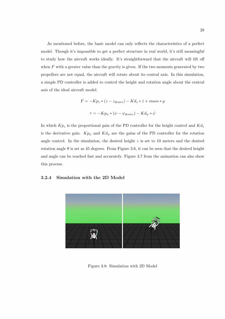
3.2.4 Simulation with the 2D Model

Figure 3.8: Simulation with 2D Model

29

Figure 3.9: Flight Trajectory with Different values of the Offset e

From the analysis of the 2D model, it can be predicted that the aircraft will rotate about

its y axis and fly towards one side when it lifts off. The simulation result (Figure 3.8) shows

this prediction is correct.

Figure 3.9 shows light trajectories of the aircraft with different values of the offset e.

The shape of the three curves are very similar. This indicates that under the influence of

mass center offset, the aircraft will fly towards one side while lifting off, and after arriving at

the peak point it starts to fly downwards even though the thrust keeps constant during the

entire process. But the difference among these figures is that the peak height is different.

When the offset is 0.0001 meter, the aircraft can reach a height of about 35 meters. When

the offset increases to 0.001 meter, the aircraft can only reach a height of about 3.5 meters.

In the last figure when the offset is 0.01 meter, the aircraft can only lift to less than 1 meter,

which means the aircraft will fall to the ground directly when the thrust is given.

30

From the above simulations, it can be concluded that the performance of the aircraft

is very sensitive to the offset of the mass center. Even small offsets can result in big

angular velocity about y axis of the robot when it lifts off from the ground. Even with the

consideration of other factors, such as air resistance force, which can reduce this sensitivity,

it’s still not a easy task to make the aircraft fly over 30 meters. Obviously this kind of

behavior is not desired.

3.2.5 Simulation with the 3D Model

The simulation with 3D model is much more complex but can reflect the behavior of

the aircraft more precisely. The following simulations mainly help to study how the self-

rotation about central axis and the offset of mass center can affect the flight performance

of the aircraft together.

Flight Trajectory with Only Rotation about Central Axis

Figure 3.10: Simulation of the Aircraft with Only Rotation about Center Axis

31

In this simulation, the offset e is set to be zero and only a small rotation moment τ is

given to the system. Thus this experimental configuration is the same with that using the

basic model. Result of the simulation (Figure 3.10)is also very similar to the result using

the basic model shown in Figure 3.7. Figure 3.10 shows that the aircraft lifts off straightly

and rotate about its central axis at the same time.

Flight Trajectory with Only Offset of Mass Center

This simulation assumes there is no self-rotation about the central axis. That is the

rotation moment τ is set to be zero. With this condition, the situation is the same the that

of a 2D model. Thus it’s not a surprise that the simulation result (shown in Figure 3.11)is

the same with the result using the 2D model in Figure 3.8. The aircraft will fly towards

one side and finally fall to the ground.

Figure 3.11: Simulation of the Aircraft with Only Offset of the Mass Center

32

Flight Trajectory with Small Angular Acceleration about Central Axis (τ = 0.15)

when offset e = 0.01m

For a real aircraft model, the value of the mass center offset does not changes once

all components are fixed. And effects from this offset on the flight have been studied in

Section 3.2.4. The rest two simulations investigates how the self-rotation about central axis

can influence the flight trajectory of the aircraft when the offset of mass center is constant.

In this simulation, the offset e is set to be 0.01 meter and the rotation moment is set to be

0.15 N ·m. From the result (Figure 3.12), it can be seen that the rotation about central

axis helps to increase the stability of the aircraft and the aircraft can lift off the ground

above 30 meters even when there is an offset of the mass center. Compared with the peak

height of about 3.5 meter shown in Figure 3.9 when the offset is also 0.01 meter without

the self-rotation, the flight performance has been greatly improved.

Figure 3.12: Simulation of the Aircraft when τ = 0.15 and e=0.01m

33

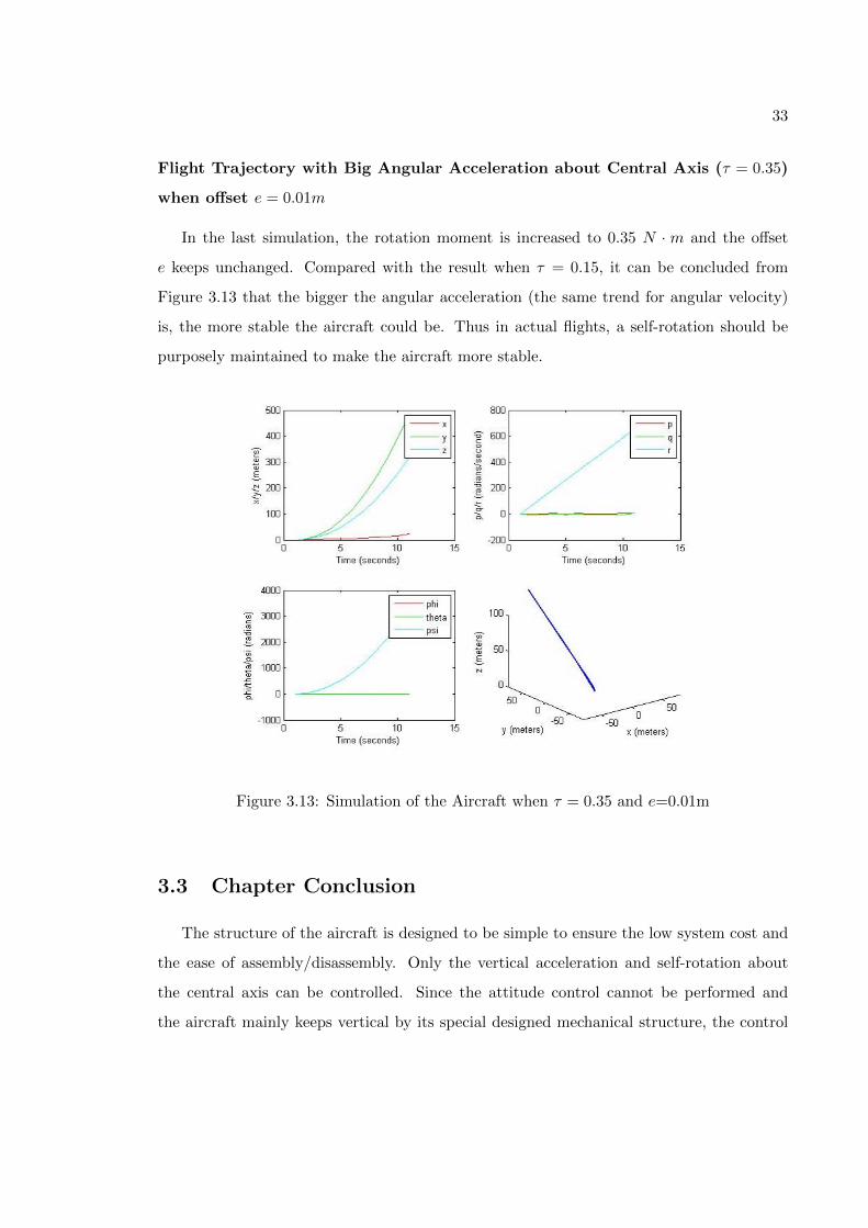
Flight Trajectory with Big Angular Acceleration about Central Axis (τ = 0.35)

when offset e = 0.01m

In the last simulation, the rotation moment is increased to 0.35 N · m and the offset

e keeps unchanged. Compared with the result when τ = 0.15, it can be concluded from

Figure 3.13 that the bigger the angular acceleration (the same trend for angular velocity)

is, the more stable the aircraft could be. Thus in actual flights, a self-rotation should be

purposely maintained to make the aircraft more stable.

Figure 3.13: Simulation of the Aircraft when τ = 0.35 and e=0.01m

3.3 Chapter Conclusion

The structure of the aircraft is designed to be simple to ensure the low system cost and

the ease of assembly/disassembly. Only the vertical acceleration and self-rotation about

the central axis can be controlled. Since the attitude control cannot be performed and

the aircraft mainly keeps vertical by its special designed mechanical structure, the control

34

Figure 3.14: Flight Test

algorithm is not simulated in this part of work. Actually in the real flight tests conducted

by the IPASS team, the aircraft is controlled in an open loop. The thrust is increased when

the user wants to get the aircraft lifting off and the thrust is decreased when the user wants

to land the aircraft.

Figure 3.14 shows the flight attitude of the aircraft after lifting off. In the left picture,

there is self-rotation about central axis and the aircraft flies toward one side and hit the

ground very soon. In the right picture, a self-rotation is added when the aircraft takes off.

It can be seen that the aircraft has a less tendency to fly towards one side. The results

of these two flight tests are coincident with the simulation shown in Figure 3.11,3.9 and

Figure 3.13.

In conclusion, this chapter illustrates the modeling of the aircraft and develops three

models in different complexity models. With these models, the dynamical characteristics

are studied and how the offset of mass center and the self-rotation about central axis affect

the flight trajectory is revealed. For follow-up works of IPASS project, the full 3D model

can be used for the design of flight control algorithms.

35

Chapter 4

Image Stitching

In the IPASS project, the aircraft needs to lift off to a specific height and take pictures

of the ground. To get a wider view of the battlefield, three cameras are installed on the

aircraft. These cameras take pictures from different view angles at the same time and the

three output images will be stitched into one panorama for the convenience of observation for

users. In this chapter, a general feature-based method for image stitching is first introduced

concisely. And for this special situation of image stitching on a mobile robot for surveillance,

a stitching method using homography is studied.

4.1 Image Formation

Before studying how to stitch images, it would be helpful to first understand how a

particular image is formed from a camera. To describe this image formation process, a

camera model needs to be established and the pinhole camera model is one of the most

commonly used one for representing perspective cameras, as shown in Figure 4.1. In real

world applications, an imaging system usually includes a set of optical lens to get better

overall image performance. In such a system, the central axis of the lens is equivalent to

the optical axis of the pinhole camera model. Though the pinhole camera model is only

a simplified model of the imaging system, the accuracy has been proven good enough to

describe the image formatting process in most practical applications.

To describe the relative position and orientation between the image plane and the scene

36

Figure 4.1: Pinhole Camera Model

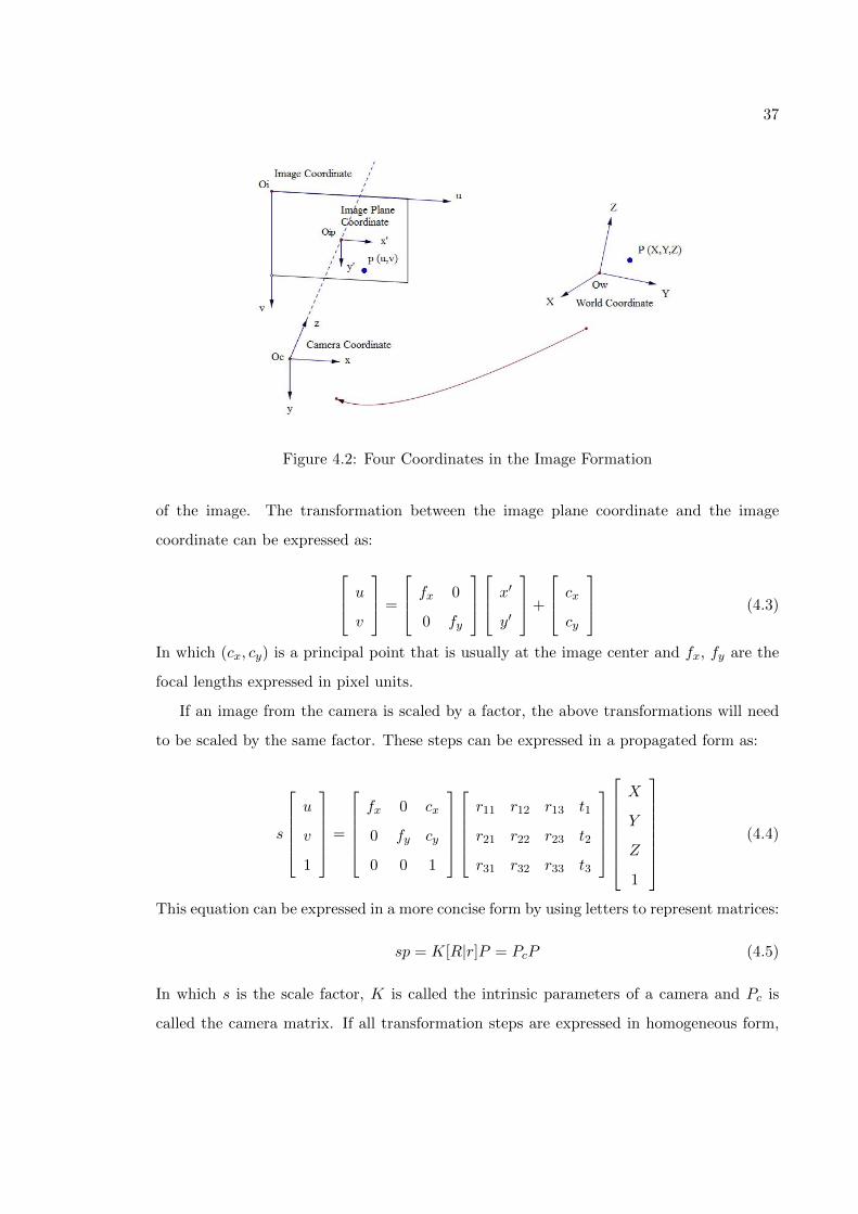
plane quantitatively, four coordinates are introduced: the world coordinate, the camera

coordinate, the image plane coordinate and the image coordinate (shown in Figure 4.2).

A point P in the world coordinate can be projected onto an image coordinate plane after

several steps. The camera coordinate is fixed with respect to the camera. The relative

position between this camera coordinate and the world coordinate can be expressed with a

translation matrix t and a rotation matrix R. (R, t) is also called extrinsic parameters of a

camera. Assume there is a point P (X,Y, Z) in the world coordinate. Then this point can

be expressed in the camera coordinate as:

x

y

z

= R

X

Y

Z

+ t (4.1)

The origin of the image plane coordinate is usually chosen at the center of the image

plane. According to the perspective projection, the point P in the camera coordinate can

be projected to the image plane as: x′

y′

=

x/z

y/z

(4.2)

The image coordinate is measured in pixels. Its origin is chosen as the top-left point

37

Figure 4.2: Four Coordinates in the Image Formation

of the image. The transformation between the image plane coordinate and the image

coordinate can be expressed as:

u

v

=

fx 0

0 fy

x′

y′

+

cx

cy

(4.3)

In which (cx, cy) is a principal point that is usually at the image center and fx, fy are the

focal lengths expressed in pixel units.

If an image from the camera is scaled by a factor, the above transformations will need

to be scaled by the same factor. These steps can be expressed in a propagated form as:

s

u

v

1

=

fx 0 cx

0 fy cy

0 0 1

r11 r12 r13 t1

r21 r22 r23 t2

r31 r32 r33 t3

X

Y

Z

1

(4.4)

This equation can be expressed in a more concise form by using letters to represent matrices:

sp = K[R|r]P = PcP (4.5)

In which s is the scale factor, K is called the intrinsic parameters of a camera and Pc is

called the camera matrix. If all transformation steps are expressed in homogeneous form,

38

then this process can be easily reversed.

Pc =

K 0

0T 1

R t

0T 1

⇒ p ∼ PcP , P ∼ Pc−1p (4.6)

In the above equation, Pc and p are the homogeneous form of Pc and p.

With these transformations, a point in the world coordinate can be easily related to a

point in the image coordinate.

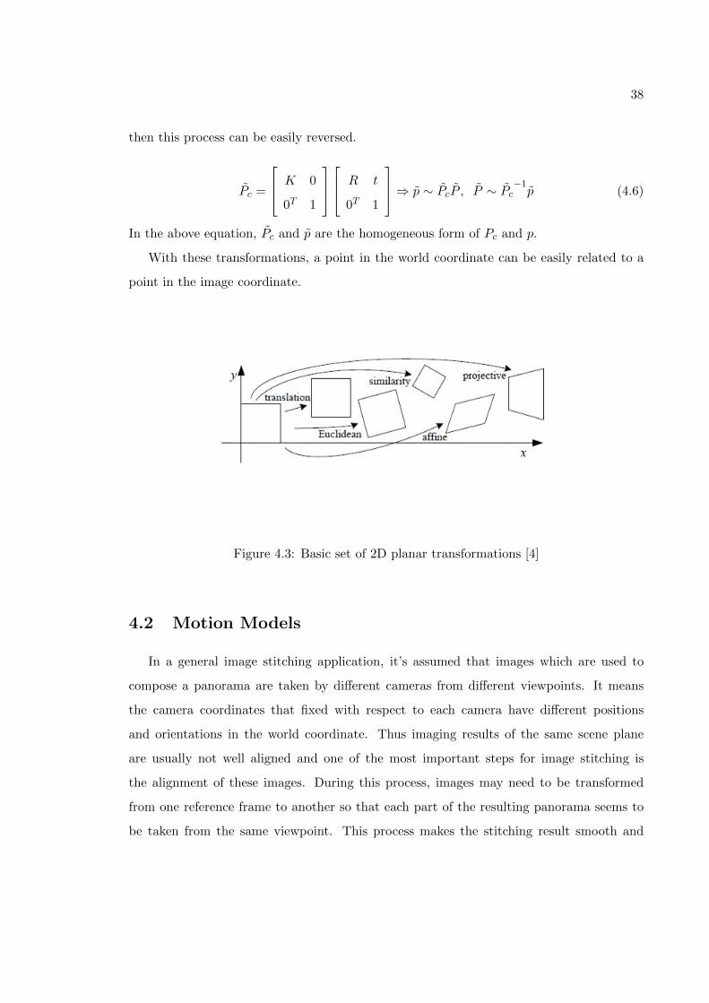
Figure 4.3: Basic set of 2D planar transformations [4]

4.2 Motion Models

In a general image stitching application, it’s assumed that images which are used to

compose a panorama are taken by different cameras from different viewpoints. It means

the camera coordinates that fixed with respect to each camera have different positions

and orientations in the world coordinate. Thus imaging results of the same scene plane

are usually not well aligned and one of the most important steps for image stitching is

the alignment of these images. During this process, images may need to be transformed

from one reference frame to another so that each part of the resulting panorama seems to

be taken from the same viewpoint. This process makes the stitching result smooth and

39

natural. Motion models are the foundations of image alignment. With these models, the

position and orientation of a picture can be expressed and transformed, which makes the

alignment very convenient.

Figure 4.4: Hierarchy of 2D coordinate transformations [4]

Some common 2D planar transformations are illustrated in Figure 4.3. The matrices of

these transformations and the characteristics that each transformation preserves are shown

in Figure 4.4. If the parameters of involved transformation matrices can be estimated,

then the original image can be transformed to a new reference frame with these matrices.

Among these transformations, perspective transformation is most important one for image

stitching. It is used in both stitching methods introduced in the following sections.

4.3 Feature-based Image Stitching

Generally there are mainly two steps for a complete stitching process: registration and

compositing. A pipeline is shown in Figure 4.5. Since for a general purpose image stitching

application, input images may be taken by different cameras with different sizes, they

are first resized to be ready for further processing. The most important part of work in

the registration step is to estimate the motion parameters of each image. After getting

registration data from this step, images will be aligned and warped into a selected plane

40

to get a rough panorama. Then exposure compensation and blending will be done to make

the rough panorama smooth and seam-free.

Figure 4.5: Pipeline of Feature-based Stitching Method from OpenCV Library

4.3.1 Feature-based Registration

As mentioned before, image alignment is one of the most fundamental works for image

stitching. To some degree, the performance of alignment determines the final stitching

result. In recent years, feature-based alignment has become a very popular method. The

idea of feature-based alignment is very intuitive. Assume two images are given to a person

and the goal is to compose the two images into a panorama. It’s natural for the person to

first compare the two images and then try to find correspondences between them. Based

on the comparison of the correspondences, the relative position and orientation of the two

images can be roughly estimated. By relocating the two images, a basic panorama can be

acquired. The idea is the same for the feature-based alignment.

41

Image Acquisition

The configuration of cameras in IPASS is shown in Figure 2.3. To study the image

stitching methods, another test frame is built and two Microsoft webcams are installed on

this frame (shown in Figure 4.6). Since commercial webcams have better driver support

and the frame is more portable than the electronic box of IPASS, which contains a lot of

unrelated stuffs, this testing set is very convenient for the study of image stitching. This

frame keeps the two cameras with a specific angle and the structural configuration is very

similar to that of IPASS. Thus the same stitching method that works with these cameras

should be easy to be applied on IPASS.

Figure 4.6: Test Frame with Two Microsoft Webcams

Figure 4.7 shows two images taken by the two cameras. It can be seen that the two

pictures are taken from different view angles but there exists an overlap area. Such overlap

area is the imaging result of the same part of scene plane but from a different view angle. It’s

obvious that the two pictures cannot be stitched together without necessary transformation.

Feature detection

After input images are acquired, the next step is to find correspondences between the

two images. Since images are stored as pixel values in the memory, a computer cannot

see and analyze images like what human beings can do. For images in Figure 4.7, each

42

Figure 4.7: Original Images Taken by the Two Cameras

image consists of 640*480 pixels. Each pixel value is a vector of numbers that represent

the color of that image point. Thus a numerical method must be found to extract useful

information from these numbers. Feature detection is widely used in many computer vision

applications. For image stitching, specific locations, such as corners of the house and the

road, are usually worth of more attention. “These kinds of localized feature are often called

keypoint features or interest points and are often described by the appearance of patches

of pixels surrounding the point location. ” [6] A good feature detection algorithm should

find robust features from images of a scene taken by different cameras. For example, the

features are expected to be scale and rotation invariant so that the same interesting point

can be easily found from images that have different scale and rotation angles.

There have been several feature detection methods available so far. Some commonly

used ones are Harris Corners Detector, Scale Invariant Feature Transform (SIFT) method,

Speeded Up Robust Features (SURF) method. Figure 4.8 show feature points detected

from the two original images with SURF detector.

43

Figure 4.8: SURF Feature Points in the Two Images

Feature Matching

Once features points are detected, the next problem is how to match these features.

Actually each feature extraction algorithm not only detects special points but also provides

a descriptor to describe each point. Feature pairs can be matched with these descriptors.

Figure 4.9 shows matched feature pairs between the two image inputs. It can be seen that

most features are correctly matched and these pairs all exist in the overlap area.

Parameter Estimation

From Section 4.1 and Section 4.2, it’s known that each image has its own reference

frame but through appropriate transformations, one image can be transformed from its

own coordinate to another. If a panorama consists of several images, one just needs to

pick up an image as a reference and transform other images to this image reference frame.

Such transformation is usually known as homography. Homography relates two image

planes and can be used to transform one image to the frame of another. The 3 by 3

44

Figure 4.9: Matching of SURF Feature Points

matrix H =

h11 h12 h13

h21 h22 h23

h31 h32 h33

can be estimated from at least 3 correspondences between

two images using functions provided by OpenCV. More details about homography will be

introduced in the following section. Chapter 13 of [5] introduces how this calculation of

homography can be achieved from the aspect of multi-view geometry.

4.3.2 Compositing

After having registered all of the input images with respect to each other, it’s time

to decide how to produce the final stitched image. As mentioned in Section 4.3.1, this

step involves selecting a reference image and a compositing surface. For applications like

IPASS, it’s reasonable to choose the image from the camera that locates in the center as the

reference. Since the number of input images are usually very limited in such applications,

for example the number is three in IPASS, it’s natural to directly transform other images

to the reference coordinate system and get all images wrapped into a flat panorama. Since

the projection onto the final surface is still a perspective projection, straight lines remain

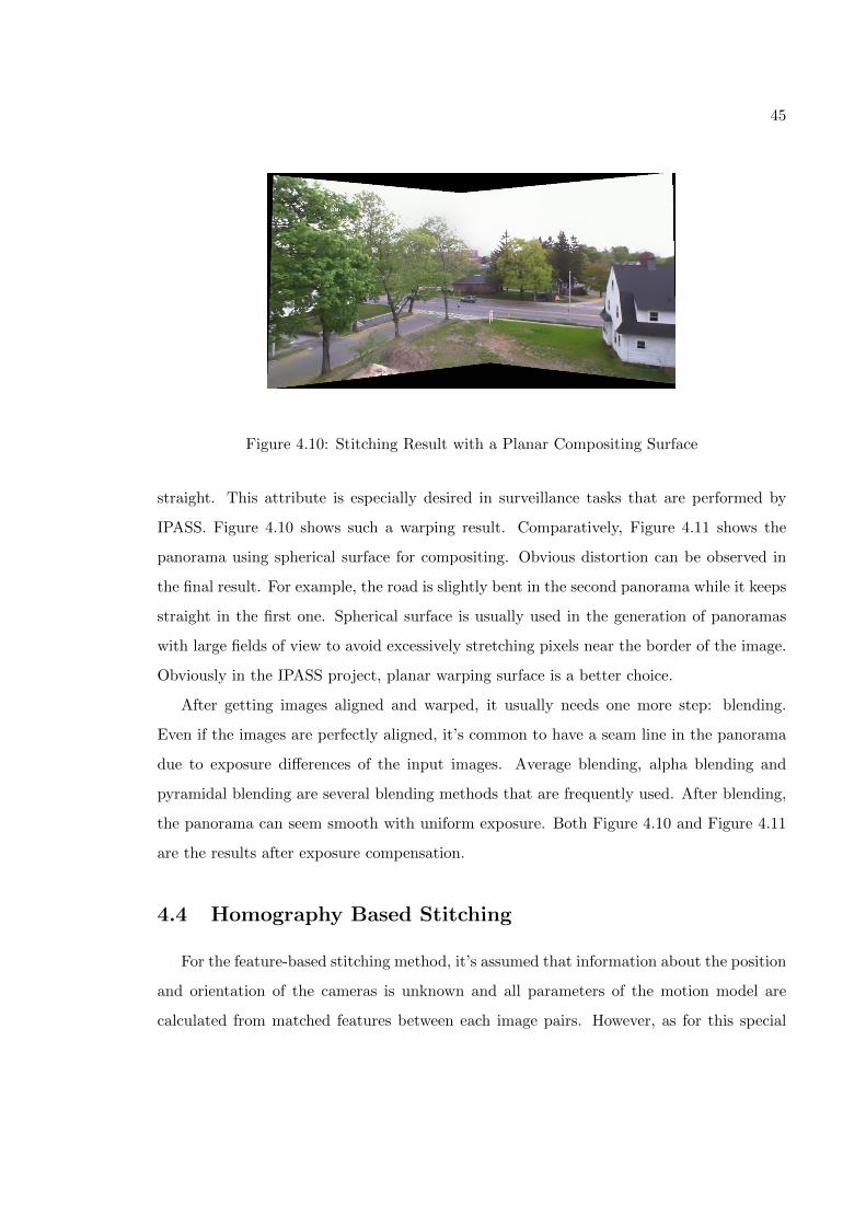
45

Figure 4.10: Stitching Result with a Planar Compositing Surface

straight. This attribute is especially desired in surveillance tasks that are performed by

IPASS. Figure 4.10 shows such a warping result. Comparatively, Figure 4.11 shows the

panorama using spherical surface for compositing. Obvious distortion can be observed in

the final result. For example, the road is slightly bent in the second panorama while it keeps

straight in the first one. Spherical surface is usually used in the generation of panoramas

with large fields of view to avoid excessively stretching pixels near the border of the image.

Obviously in the IPASS project, planar warping surface is a better choice.

After getting images aligned and warped, it usually needs one more step: blending.

Even if the images are perfectly aligned, it’s common to have a seam line in the panorama

due to exposure differences of the input images. Average blending, alpha blending and

pyramidal blending are several blending methods that are frequently used. After blending,

the panorama can seem smooth with uniform exposure. Both Figure 4.10 and Figure 4.11

are the results after exposure compensation.

4.4 Homography Based Stitching

For the feature-based stitching method, it’s assumed that information about the position

and orientation of the cameras is unknown and all parameters of the motion model are

calculated from matched features between each image pairs. However, as for this special

46

Figure 4.11: Stitching Result with a Spherical Compositing Surface

stitching application on a mobile robot, cameras are fixed on the base. The relative position

and orientation of the cameras can be acquired and will not change after installed. These

information can be used to stitch images.

4.4.1 Homography

Homography relates points on two image planes, which are the images of the same scene

plane from different viewpoints, as shown in Figure 4.12. It’s said that the plane induces

a homography between the views. In Figure 4.12, the point xπ on scene plane π can be

projected to two image planes as x and x′. As illustrated in Section 4.1, the following two

perspectivities can be derived: x = H1πxπ and x′ = H2πxπ. The composition of the two

perspectivities is the homography between the image planes: x′ = H2πH−11π xπ = Hx.

[5] describes how to get the homography with a calibrated stereo rig. It’s supposed that

the world origin is at the first camera and the two camera matrices are:

PE = K[I|0], P ′E = K ′[R|t]

K and K ′ are the intrinsic matrices of the two cameras. The world plane πE has coordinates

πE = (nT , d)T so that for points on the plane, nT X + d = 0. Then the resulting induced

homography is

47

Figure 4.12: Homography between Two Image Planes [5]

H = K ′(R− tnT /d)K−1 (4.7)

In the above equation, K and K ′ are camera intrinsic parameters of the two cameras, R

and t are rotation and translation matrices between the two cameras.

If the relative position between the scene plane and the two cameras are fixed, the

homography can be calculated and keeps constant. Then it can be applied to image pairs

captured by cameras on the mobile robot. Since the calculation of homography can be

offline, it will greatly reduce the time for stitching images. As to the IPASS, there are three

cameras installed onboard. The transformations are demonstrated in Figure 4.13. Since

the image plane from the middle camera is parallel to the scene plane, it’s chosen as the

reference plane and the other two image planes are transformed to its frame.

4.4.2 Plane induced parallax

Homography between two images can be calculated from three point correspondences.

[5] explains how this can be accomplished. OpenCV provides a function that can do this

with the input of an array of point correspondences. Since the corners of a chessboard are

very easy to detect and their coordinates can be calculated accurately, it should be a good

choice for homography calculation. Figure 4.14 shows the image pair of an 8∗6 chessboard.

48

Figure 4.13: Transformations of Three Cameras with Homography

With OpenCV, the corners are detected and marked with color points and lines.

The homography that maps the right image to the left is calculated from these corners:

H =

0.5156680583284313 −0.0468482202080017 385.4620354397438

−0.1267729459760625 0.9022901489228606 12.17586065380672

−0.0007495973635153077 3.324550187583125e− 005 1

Keep the cameras fixed on the table and take several more image pairs. Each time the

chessboard is placed on different planes in the space. In Figure 4.15, the chessboard remains

the same plane from which the homography is induced. The middle image of Figure 4.15

shows the perspective transformation result after the homography is applied to the right

image. And the bottom image shows the result of the alignment of the two images. Since

exposure compensation is not done, there is an obvious seem line in the rough panorama.

But it can be seen that the chessboard is stitched together very well. In Figure 4.16, the

chessboard is placed on different planes , and obvious misalignment can be found on the

chessboard in both of the alignment results.

49

Figure 4.14: Chessboard with Corners Marked by Color Circles and Lines

This phenomenon is called plane induced parallax. That’s because a homography only

relates two image planes of the same scene plane while the camera is taking the picture of a

3D scene. Thus if an object is not on the same scene plane that induces the homography, it

cannot be aligned well from two images. From Equation 4.7 H = K ′(R− tnT /d)K−1, this

can be easily explained mathematically. Besides intrinsic parameters and relative position

and orientation of the two cameras, a homography is also determined by the parameters n

and d, which define the scene plane π. So if n and d change, the old homography cannot

be applied for the alignment any more.

Obviously, this is not what’s expected. Mobile robot always needs to move around and

it’s impossible to guarantee that the camera and the interested scene plane have fixed posi-

tion. Thus more works need to be done to make this method fit for the IPASS application.

4.4.3 Infinite Homography

To avoid calculating homography every time when image stitching is performed, it’s

required to find a homography that can be applied to all image pairs through the task.

This requirement leads to another concept: infinite homography, which is defined as

50

Figure 4.15: Image Alignment using Homography (without misalignment)

H∞ = limd→∞

H = K ′RK−1 (4.8)

In this definition, H∞ holds when the orthogonal distance of the plane to the first

camera d tends to be indefinite. Fortunately, since the scene plane is usually far away from

the camera on mobile robots, for example IPASS flies to 30 meters above the ground and

then takes pictures, it can be assumed that d is very large and H∞ can be used through the

entire mission. For this infinite homography, it only depends on the rotation between the

two cameras and the intrinsic parameters, which can be acquired from camera calibration.

51

Figure 4.16: Image Alignment using Homography (with misalignment)

52

4.4.4 Camera Calibration

Calibration aims at measuring accurately the intrinsic and extrinsic parameters of the

camera model. In the IPASS project, camera calibration can be used to get intrinsic pa-

rameters and distortion coefficients of a camera. As introduced in Section 4.1, intrinsic

parameter matrix K =

fx 0 cx

0 fy cy

0 0 1

can be used to map a point in the camera coordi-

nate to the image coordinate. K is also required to get H∞. Distortion coefficients can be

used for distortion correction, which is a necessary step before images are stitched. The

idea of camera calibration is that with pixel coordinates of the image points and the 3D

coordinates of the corresponding scene points, the unknown parameters K, R and t can be

calculated by solving the perspective projection equation.

The calibration from planar grid is a very popular and practical method first proposed

by Zhang [17]. This method has been implemented in OpenCV. It requires the user to

take several pictures of the pattern shown at different positions and orientations. “By

known the 2D position of the corners on the real pattern and the pixel coordinates of their

corresponding corner on each image, the intrinsic and extrinsic parameters (including radial

and tangential distortion) are determined simultaneously by solving a least-square linear

minimization followed by a nonlinear refinement.” [6] For the two Microsoft webcams used

for testing, the parameters from the calibration are in the following:

K =

5.9488728159848e+ 002 0 3.2229015408292e+ 002

0 5.9413758210164e+ 002 2.3704855673909e+ 002

0 0 1

K ′ =

5.8720493128210e+ 002 0 3.2943841218474e+ 002

0 5.8902398093762e+ 002 2.3992898076557e+ 002

0 0 1

The above two matrices can be used to calculate the infinite homography. Since the

distortion effects have been taken good care of by the webcam, distortion correction is

not necessary for the stitching of images taken by these two cameras. But for the CMOS

53

cameras used on IPASS, the distortion is very obvious and correction is a must-do work.

The intrinsic parameters and the distortion coefficients of one of the cameras on IPASS are

calculated as:

Ki =

626.3582340881325 0 275.5833525006261

0 624.704516208163 270.6916549616896

0 0 1

distCoeffs = [−0.4575583887, 0.1473511949, 0.004305622674,−0.009150287285, 0.1797360113]

Figure 4.17: Distortion of a Camera: (a) No Distortion (b)Barrel Distortion (c) PincushionDistortion [6]

The most commonly seen distortion effects are barrel effect and pincushion effect as

shown in Figure 4.17. These two effects are the result of radial distortion, which is because

real optical lenses cannot keep straight lines straight after getting through, like what a

pinhole model does. Another kind of distortion is called tangential distortion, which occurs

because the image taking lenses are not perfectly parallel to the imaging plane. To correct

these two kinds of distortions, OpenCV uses the following formulas to model the radial and

tangential distortion respectively:

54

xcorrected = x(1 + k1r2 + k2r

4 + k3r6)

ycorrected = x(1 + k1r2 + k2r

4 + k3r6)

And

xcorrected = x+ [2p1xy + p2(r2 + 2x2)]

ycorrected = y + [p1(r2 + 2y2) + 2p2xy]

These two distortion models result to five distortion parameters: Distortioncoeffcients =

(k1, k2, p1, p2, k3). This is exactly how five numbers in the above distortion coefficients of

the IPASS camera are defined. With these distortion coefficients, pixels in the distorted

image can be remapped and the result is an undistorted image (as shown in Figure 4.18).

Figure 4.18: Distortion Correction: (Left) distorted image (Right) undistorted image

From the calibration of a single camera, the distortion of images can be corrected and

the intrinsic matrices can be acquired. But to get the infinite homography, it’s still required

55

to know the value of R. OpenCV also provides a function for stereo calibration. Based

on the calibration of each camera, this function can further calculate the relative position

and orientation of the camera pair. For the two cameras on the testing frame, the rotation

matrix is calculated as:

R =

8.7432070927900e− 001 2.4446238152751e− 002 4.8473258479912e− 001

−3.0139917703522e− 002 9.9953786573123e− 001 3.9547857435484e− 003

−4.8441189362637e− 001 −1.8067551290407e− 002 8.7465346332343e− 001

By now, all necessary parameters are known to get the infinite homography:

H∞ =

0.6188018464580525 0.01482359586021116 362.4972806330147

−0.2256518767368491 1.002286210472574 44.01416286348356

−0.0008235002191648365 −3.07148371936926e− 005 1.153767449288414

By applying this homography, one image can be transformed into the reference frame

of the other. Figure 4.19 shows a result of image stitching with this homography. It can

be seen that the alignment result is very good and the infinite homography works just as

expected.

4.5 Comparison of the Two Image Stitching Methods

Section 4.3 and Section 4.4 have introduced the feature-based image stitching and the

homography-based image stitching. Both methods can get the image stitching work done

but each of them has its own advantages and disadvantages. Figure 4.20 shows simplified

pipelines of these two methods. From the pipelines, it can be seen that the homography-

based method makes full use of the information about the relative position and orientation of

the two cameras. It calculates infinite homography offline and use this infinite homography

for the alignment of image pairs online. This makes the stitching pipeline much shorter than

that of feature-based method. As to the feature-based method, to get homography between

two images, feature detection and feature match must be finished first and with detected

correspondences homography is then estimated. These extra steps result in a much longer

stitching time.

56

Figure 4.19: Image Alignment with Infinite Homography

A software application is developed to study the performance of the two image stitching

methods. Its GUI is shown in Figure 4.21. This application is written in C++ with OpenCV

and wxWidgets libraries. There are two threads running at the same time: one takes care

of the GUI and the other is in charge of all image processing works. This application can

be used to operate cameras and capture image samples from the two cameras. Camera

calibration algorithm is also integrated into this application and it can read captured image

samples and then calculate camera parameters. Both methods are implemented in this

software and users can switch between the two methods very conveniently. If the image

stitching function is started, this application will continuously capture images and stitch

image pairs. Both the original images and the panorama can be displayed at the image

panels of the GUI. Meanwhile, update frequency of the image processing loop can be shown

in the status bar at the bottom.

Figure 4.22 shows the stitching results of the two methods. It can be seen that both

panoramas look natural and smooth. No obvious seem can be observed from either result.

57

Figure 4.20: Simplified Pipelines of Feature-based Method and Homography-based Method

There is also no outstanding misalignment that can be found. [19] and [20] discussed the

evaluation of image mosaics. But unfortunately, there is still no effective method available

so far that can evaluate panoramas quantitatively. Generally, people just evaluate stitching

results with their eyes. In this qualitative way, both panoramas look as good as expected.

Since both of the methods can stitch images well, the other main factor for comparison is

the time required for the stitching process. Table 4.1 shows several update frequency samples

taken from the software when the image stitching function is working. As illustrated above,

this frequency reflects how fast the whole image processing steps can be finished in that

thread. Actually, in this image processing thread, only image capturing and stitching run

in a sequence. And it takes very little time to capture images from the cameras. Thus

the update frequency can be roughly regarded as the update frequency of the stitching

pipeline. It’s obvious that the homography-based stitching method has a great advantage

in the stitching speed. The update frequency can be around 15Hz while it’s only about

0.35Hz for the feature-based stitching. Since IPASS only stays in the air for a very short

time around its peak height, feature-based stitching method is too slow to get captured

images by the aircraft stitched and displayed in real time on the ground station.

58

Figure 4.21: GUI of the Application for Image Stitching

Though the homography-based method has a better performance in the stitching speed

with an almost equivalent stitching result, it also has some disadvantages. For this method,

the stitching result relies on the infinite homography matrix a lot. So if this matrix is not

effective and accurate any more, the stitching process will be a mess. Since the infinite

homography is calculated offline and keeps constant through the mission, it cannot adapt

to changes of the camera configuration during the mission. If the relative position and

orientation of the camera pair changes, the camera pair must be recalibrated and the infinite

Number Feature-based Stitching Homography-based Stitching

1 0.370645 Hz 13.8889 Hz

2 0.373413 Hz 14.9254 Hz

3 0.33557 Hz 17.8571 Hz

4 0.345304 Hz 17.5439 Hz

5 0.305998 Hz 11.7647 Hz

6 0.336022 Hz 16.129 Hz

7 0.33456 Hz 13.3333 Hz

8 0.329598 Hz 15.873 Hz

Table 4.1: Update Frequency of the Two Stitching Methods

59

Figure 4.22: Comparison of Panoramas - top: feature-based method, bottom: homography-based method

homography also requires to be updated. Comparatively, the adaptability is the advantage

of the feature-based method. For the feature-based method, the stitching process does not

involve the use of information about the camera configuration. It only requires enough

overlap area between image pairs from the cameras to extract sufficient feature points for

the homography estimation. Thus as long as this kind of overlap is guaranteed, the stitching

method keeps valid even if the cameras are redistributed on the mobile robot. Moreover,

the homography-based method works under the assumption that the scene plane is very

far away from the cameras. So if images of the scene nearby the robot are required to be

stitched, distinct misalignment will occur in the panorama generated by the homography-

based method. But for feature-based method, there is no such restriction.

From the above comparisons, the following conclusions can be drawn: if a application

requires fast stitching speed and the interested scene plane is far from the cameras, the

60

homography-based image stitching method is a good choice; if a application has no require-

ments for stitching speed, then the feature-based method is the first choice for its reliability

and adaptability. There are many restrictions on the use of the homography-based image

stitching method. But once this method can be used, it can provide a great advantage in

the stitching speed as well as satisfying quality of panoramas.

61

Chapter 5

Conclusion and Future Work

This thesis first presented the purpose of the IPASS project and gives a detailed de-

scription of the system requirements. Then the system design of IPASS project is briefly

introduced. This part includes both of the mechanical and electronic design of the aircraft.

Software development is also presented. The main body of the thesis is the modeling and

simulation of the aircraft and image stitching. Three dynamic models at different complex-

ity levels are derived and simulated in Matlab. With these models, dynamical characteristics

of the aircraft, including how the offset of mass center and the self-rotation about central

axis affect the flight trajectory, are studied. In the image stitching part, two methods of

image stitching are discussed. The feature-based stitching method is concisely introduced

and the homography-based method is studied with details. Moreover, the image formation

process and camera calibration are also illustrated. Both of the methods are implemented

and the result shows the homography-based method can stitch images with a faster speed

and little compromise in the quality of the panorama.

While the whole system has been fully developed and different image stitching methods

have been implemented and compared, there is still a lot of work to be completed in im-

proving both the flight performance and the quality and speed of image stitching. To ensure

the portability and the ease of operation, the aircraft was designed to be capable of vertical

taking off and vertical landing without attitude control. However, the simulation results

in Chapter 3 shows that this design has brought great difficulties in the flight trajectory

62

control. The situation can be even worse if the aircraft is operated in bad weathers. In the

future, the aircraft might be improved with more degrees of maneuverability to improve

its flight performance. The cameras installed on IPASS are low-cost CMOS cameras. The

quality of images taken by these cameras are not good enough and this sometimes leads to

failure to extract enough feature points for the feature-based image stitching method. In

future works, these devices might need to be upgraded. For the homography-based method,

exposure compensation hasn’t been done in this project. And if the distance between the

robot and the scene plane is not far enough, obvious misalignment of the images will oc-

cur. The homography-based image stitching is still far from perfect. Moreover, except the

modeling and image stitching, other open problems presented in Section 2.5 still need to be

solved. In short, there are still many works to be done for the IPASS project.

63

Bibliography

[1] “Factsheets: Wasp iii small unmanned aircraft system.” http://www.af.mil/

information/factsheets/factsheet.asp?id=10469, Jan. 2013.

[2] “Factsheets: The rq-11 raven small unmanned aircraft system.” http://www.af.mil/

information/factsheets/factsheet.asp?fsID=10446, Sept. 2011.

[3] “Wikipedia: Introduction to honeywell rq-16 t-hawk.” http://en.wikipedia.org/

wiki/Honeywell_RQ-16_T-Hawk.

[4] R. Szeliski, Computer Vision: Algorithms and Applications. Springer, 2010.

[5] R. Hartley and A. Zisserman, Multiple View Geometry in Computer Vision. Cambridge

University Press, 2004.

[6] R. Siegwart, Introduction to Autonomous Mobile Robots. MIT Press, 2nd ed., 2011.

[7] “Honeywell brochure: Rq-16 t-hawk.” http://www51.honeywell.com/aero/common/

documents/myaerospacecatalog-documents/Defense_Brochures-documents/

T-Hawk_Unmaned_Micro_Air_Vehicle.pdf, June 2010.

[8] “Cost of existing uav systems - military equipment.” http://nationsdawnofanera.

weebly.com/-unmanned-aircraft.html.

[9] A. Blumenau, A. Ishak, B. Limone, Z. Mintz, C. Russell, A. Sudol, R. Linton, L. Lai,

T. Padir, and R. V. Hook, “Design and implementation of an intelligent portable aerial

surveillance system (ipass),”

[10] R. W. Beardk, “Quadrotor dynamics and control,” tech. rep.

64

[11] N. Michael, D. Mellinger, Q. Lindsey, and V. Kumar, “The grasp multiple micro-uav

testbed,” Robotics Automation Magazine, IEEE, vol. 17, pp. 56–65, sept. 2010.

[12] I. Zohar, A. Ailon, and H. Guterman, “An automatic stabilization system for quadro-

tors with applications to vertical take-off and landing,” in AUVSI-IEEE Joint Confer-

ence, Israel, 2010.

[13] R. L. Pedro Castillo and A. E. Dzul, Modelling and Control of Mini-Flying Machines.

[14] J. Mehta and S. Bhirud, “Image stitching techniques,” in Thinkquest 2010 (S. Pise,

ed.), pp. 74–80, Springer India, 2011.

[15] M. Brown and D. Lowe, “Automatic panoramic image stitching using invariant fea-

tures,” International Journal of Computer Vision, vol. 74, no. 1, pp. 59–73, 2007.

[16] R. Szeliski, “Image alignment and stitching: A tutorial,” Foundations and Trends in

Computer Graphics and Vision, vol. 2, pp. 1–104, 2006.

[17] Z. Zhang, “A flexible new technique for camera calibration,” Pattern Analysis and

Machine Intelligence, IEEE Transactions on, vol. 22, no. 11, pp. 1330–1334, 2000.

[18] R. Szeliski, Learning OpenCV : computer vision with the OpenCV library. Sebastopol,

CA : O’Reilly, 2008.

[19] J. Boutellier, O. Silvn, M. Tico, and L. Korhonen, “Objective evaluation of image mo-

saics,” in Computer Vision and Computer Graphics. Theory and Applications (J. Braz,

A. Ranchordas, H. Arajo, and J. Pereira, eds.), vol. 21 of Communications in Computer

and Information Science, pp. 107–117, Springer Berlin Heidelberg, 2009.

[20] P. Paalanen, J. k. Kmrinen, H. Klviinen, P. Paalanen, J. k. Kamarainen, and H. Klvi-

inen, “Image based quantitative mosaic evaluation with artificial video.”

65

Appendix A

Appendix A: Matlab Simulation

Code for the 3D Model

A.1 simulation.m

%−−−−−−−−−−−−−−−−−−− s imu la t i on con t r o l −−−−−−−−−−−−−−−−−−−−%

% Simulat ion f o r Ipas s

% Ruixiang 01/27/2013

%−−−−−−−−−−−−−−−−−−−−−−−−−−−−−−−−−−−−−−−−−−−−−−−−−−−−−−−−−−−%

%c l e a r

clear ;

close a l l ;

clc ;

%Desired system s t a t e

he ight =15; %des i r ed h e i g h t o f the a i r c r a f t

yaw=45/180∗pi ; %des i r ed yaw ang le o f the a i r c r a f t

%So lve the ord inary d i f f e r e n t i a l equat ion f o r x

66

totalTime =10;

tspan =0:1: totalTime ;

x0=zeros ( 1 2 , 1 ) ;

[ t , x]=ode45 (@( t , x ) i p a s s ( t , x , height , yaw ) , tspan , x0 ) ;

%−−−−−−−−−−−−−−−−−−−−−−− Animation −−−−−−−−−−−−−−−−−−−−−−−−−%

% ATTENTION: I f you don ’ t have 3D Animation Toolbox i n s t a l l e d

% in Matlab , you need to d i s a b l e t h i s par t o f code to run

% the s imu la t i on

%Rotat ion Matrix

% −−phi−−−−r o t a t i on ang le about x a x i s

% −−the ta−−r o t a t i on ang le about y a x i s

% −−psi−−−−r o t a t i on ang le about z a x i s

syms phi theta p s i

Rxyz=[cos ( p s i )∗ cos ( theta )−sin ( phi )∗ sin ( p s i )∗ sin ( theta )

−cos ( phi )∗ sin ( p s i )

cos ( p s i )∗ sin ( theta )+cos ( theta )∗ sin ( phi )∗ sin ( p s i ) ;

cos ( theta )∗ sin ( p s i )+cos ( p s i )∗ sin ( phi )∗ sin ( theta )

cos ( phi )∗ cos ( p s i )

sin ( p s i )∗ sin ( theta )−cos ( p s i )∗ cos ( theta )∗ sin ( phi ) ;

−cos ( phi )∗ sin ( theta ) sin ( phi ) cos ( phi )∗ cos ( theta ) ] ;

Rx=[1 0 0 ; 0 cos(−pi /2) −sin(−pi / 2 ) ;

0 sin(−pi /2) cos(−pi / 2 ) ] ;

world=vrworld ( ’ a i r c r a f t 3 d f a r . wrl ’ ) ;

open ( world ) ;

67

f i g=v r f i g u r e ( world ) ;

x s i z e=s ize ( x ) ;

N=x s i z e ( 1 ) ;

set ( world , ’ RecordMode ’ , ’ scheduled ’ ) ;

set ( world , ’ RecordInte rva l ’ , [ 1 ,N ] ) ;

set ( f i g , ’ Record2DFileName ’ , ’ i pa s s 3d2 . av i ’ ) ;

set ( f i g , ’ Record2D ’ , ’ on ’ ) ;

set ( f i g , ’ Record2DCompressQuality ’ , 1 0 0 ) ;

set ( f i g , ’ NavPanel ’ , ’ none ’ ) ;

T=600; %Generate T animation

i f N/T<1

step =1;

else

s tep=N/T;

end

index =1;

for t =1: s tep :N

world . a i r c r a f t . t r a n s l a t i o n =[x ( index , 1 )

x ( index , 3 ) x ( index , 2 ) ] ;

world . a i r c r a f t . r o t a t i o n=

vrrotmat2vec (Rx∗ subs (Rxyz , [ phi , theta , p s i ] ,

[ x ( index , 1 0 ) , x ( index , 1 1 ) , x ( index , 1 2 ) ] ) ) ;

index=round( index+step ) ;

i f index>N

index=N;

end

68

set ( world , ’Time ’ , t ) ;

vrdrawnow ;

pause ( 0 . 5 ) ;

i f x ( index ,3)<0

break ;

end

end

close ( world ) ;

%−−−−−−−−−−−−−−−−−−−−−− Draw Figure −−−−−−−−−−−−−−−−−−%

%f i g u r e (1)

subplot ( 2 , 2 , 1 ) ;

%p l o t ( x ( : , 3 ) ) ;

plot ( x ( : , 1 ) , ’ r ’ ) ;

hold on

%p l o t ( x ( : , 1 1 ) , ’ y ’ ) ;

plot ( x ( : , 2 ) , ’ g ’ ) ;

plot ( x ( : , 3 ) , ’ c ’ ) ;

% p l o t ( x ( : , 6 ) , ’ b ’ ) ;

hold o f f

xlabel ( ’Time ( seconds ) ’ ) ;

ylabel ( ’ x/y/z ( meters ) ’ ) ;

legend ( ’ x ’ , ’ y ’ , ’ z ’ ) ;

%f i g u r e (2)

subplot ( 2 , 2 , 2 )

%p l o t ( x ( : , 3 ) ) ;

plot ( x ( : , 7 ) , ’ r ’ ) ;

69

hold on

%p l o t ( x ( : , 1 1 ) , ’ y ’ ) ;

plot ( x ( : , 8 ) , ’ g ’ ) ;

plot ( x ( : , 9 ) , ’ c ’ ) ;

% p l o t ( x ( : , 6 ) , ’ b ’ ) ;

hold o f f

xlabel ( ’Time ( seconds ) ’ ) ;

ylabel ( ’p/q/ r ( rad ians / second ) ’ ) ;

legend ( ’p ’ , ’ q ’ , ’ r ’ ) ;

%f i g u r e (2)

subplot ( 2 , 2 , 3 )

%p l o t ( x ( : , 3 ) ) ;

plot ( x ( : , 1 0 ) , ’ r ’ ) ;

hold on

%p l o t ( x ( : , 1 1 ) , ’ y ’ ) ;

plot ( x ( : , 1 1 ) , ’ g ’ ) ;

plot ( x ( : , 1 2 ) , ’ c ’ ) ;

% p l o t ( x ( : , 6 ) , ’ b ’ ) ;

hold o f f

xlabel ( ’Time ( seconds ) ’ ) ;

ylabel ( ’ phi / theta / p s i ( rad ians ) ’ ) ;

legend ( ’ phi ’ , ’ theta ’ , ’ p s i ’ ) ;

%Plot t r a j e c t o r y

%f i g u r e (3)

subplot ( 2 , 2 , 4 )

plot3 ( x ( : , 1 ) , x ( : , 2 ) , x ( : , 3 ) , ’−b ’ , ’ LineWidth ’ , 2 )

axis ([−80 80 −80 80 0 1 0 0 ] )

70

xlabel ( ’ x ( meters ) ’ ) ;

ylabel ( ’ y ( meters ) ’ ) ;

zlabel ( ’ z ( meters ) ’ ) ;

%−−−−−− end −−−−−−%

A.2 ipass.m

%−−−−−−−−−−−−−−−−−−−− a i r c r a f t model −−−−−−−−−−−−−−−−−−−−−%

% Simulat ion f o r Ipas s

% Ruixiang 01/27/2013

%−−−−−−−−−−−−−−−−−−−−−−−−−−−−−−−−−−−−−−−−−−−−−−−−−−−−−−−−−%

% This func t i on d e s c r i b e s the model and con t r o l law

% of the a i r c r a f t .

% It ’ s assumed t ha t the mass cen te r i s r i g h t on the

% v e r t i c a l cen te r a x i s .

function xdot = i p a s s ( t , x , he ight , yaw)

%Model Parameters

mass =1.67; % 1.67 kg

%1 pound ∗ ( square inch ) = 0.292639653 gram ∗ ( square meter )

I z z =0.00534; % 0.00534 kg∗mˆ2 = 18.25 l b ∗ inch ˆ2 , from So l idworks

Iyy =0.0122; % 41.75 l b ∗ inch ˆ2

Ixx =0.0122;

e =0.01; % 0.01 m

%h=0.163; % 0.163 m

%l=s q r t ( eˆ2+h ˆ2) ;

g =9.8 ; % Grav i t a t i ona l a c c e l e r a t i on in m/s ˆ2

71

I =[ Ixx 0 0 ; 0 Iyy 0 ; 0 0 I z z ] ;

%I n i t a l i z e xdot

xdot=zeros ( 1 2 , 1 ) ;

%System Input

%F1 , F2 : t h r u s t o f the two p r o p e l l e r s

%tau1 , tau2 : moment generated by the two p r o p e l l e r s

%F: t o t a l t h r u s t

%tau : t o t a l moment

F1=16;

F2=16;

tau1 =0;

tau2 =0.35;

F=F1+F2 ;

tau=tau1+tau2 ;

%PD con t r o l f o r Height ( z ) and Yaw( t h e t a )

%−−−−−−−−−−−−−−−−−−−−−−−−−−−−−−−−−−−−−−−−−−−−−−−−−−−

% Z des i r e =10;

% The ta de s i r e =16;

% Z de s i r e=he i g h t ;

% The ta de s i r e=yaw ;

%

% Kp z=3.5;

% Kd z=4;

% Kp theta =2.5;

% Kd theta=2;

72

%

% F=−Kp z ∗( x(1)− Z de s i r e )−Kd z∗x(2)+mass∗g ;

% tau=−Kp theta ∗( x(3)−The ta de s i r e )−Kd theta ∗x ( 4 ) ;

%−−−−−−−−−−−−−−−−−−−−−−−−−−−−−−−−−−−−−−−−−−−−−−−−−−−

% %Basic Model

% xdot (1)=x ( 2 ) ;

% xdot (2)=1/mass∗(F−mass∗g ) ;

% xdot (3)=x ( 4 ) ;

% xdot (4)=1/ I z z ∗ tau ;

% %Without cons i d e ra t i on o f s e l f r o t a t i on about v e r t i c a l cen te r

% ax i s o f a i r c r a f t

% xdot (1)=x ( 2 ) ;

% xdot (2)=1/ Iyy ∗F∗ l ∗e/ l ;

% xdot (3)=1/mass∗(F−mass∗g∗ cos ( x ( 1 ) ) ) ;

% xdot (4)=g∗ s in ( x ( 1 ) ) ;

% xdot (5)=x (3)∗ cos ( x (1))−x (4)∗ s in ( x ( 1 ) ) ;

% xdot (6)=x (3)∗ s in ( x (1))+x (4)∗ cos ( x ( 1 ) ) ;

%With cons i d e ra t i on o f s e l f r o t a t i on about v e r t i c a l cen te r a x i s o f

%a i r c r a f t

xdot (1:3)= x ( 4 : 6 ) ;

xdot (4 :6 )=[0 ;0 ; − g ]+1/mass ∗ [ cos ( x (12 ) )∗ cos ( x(11))− sin ( x (10 ) )∗ sin ( x (12 ) )∗ sin ( x ( 11 ) )

−cos ( x (10 ) )∗ sin ( x ( 12 ) ) cos ( x (12 ) )∗ sin ( x (11))+ cos ( x (11 ) )∗ sin ( x (10 ) )∗ sin ( x ( 1 2 ) ) ;

cos ( x (11 ) )∗ sin ( x (12))+ cos ( x (12 ) )∗ sin ( x (10 ) )∗ sin ( x ( 11 ) ) cos ( x (10 ) )∗ cos ( x ( 12 ) )

sin ( x (12 ) )∗ sin ( x(11))−cos ( x (12 ) )∗ cos ( x (11 ) )∗ sin ( x ( 1 0 ) ) ;

−cos ( x (10 ) )∗ sin ( x ( 11 ) ) sin ( x ( 10 ) ) cos ( x (10 ) )∗ cos ( x ( 1 1 ) ) ] ∗ [ 0 ; 0 ; F ] ;

xdot (7:9)= inv ( I ) ∗ ( [ 0 ; F∗e ; tau ]−cross ( [ x ( 7 ) ; x ( 8 ) ; x ( 9 ) ] , I ∗ [ x ( 7 ) ; x ( 8 ) ; x ( 9 ) ] ) ) ;

73

xdot (10:12)= inv ( [ cos ( x ( 11 ) ) 0 −cos ( x (10 ) )∗ sin ( x ( 1 1 ) ) ; 0 1 sin ( x ( 1 0 ) ) ; sin ( x (1 1 ) )

0 cos ( x (10 ) )∗ cos ( x ( 1 1 ) ) ] ) ∗ [ x ( 7 ) ; x ( 8 ) ; x ( 9 ) ] ;

end

%−−−−−− end −−−−−−%

74

Appendix B

Appendix B: C++ Code for

Homography-based Image

Stitching Method

B.1 homostitch.h

/∗

∗ homost i tch . h

∗

∗ Created on : Mar 23 , 2013

∗ Author : rdu

∗/

#ifndef HOMOSTITCH H

#define HOMOSTITCH H

#include ”opencv/cv . h”

#include ”wx/wx . h”

75

using namespace std ;

using namespace cv ;

class HomoStitch

{

public :

HomoStitch ( ) ;

˜HomoStitch ( ) ;

protected :

vector<Mat> m cvImages ;

Mat m stitchedImage ;

private :

Mat m transfMatr ix ;

private :

void In i tTrans fMatr ix ( ) ;

public :

void St i tchImages ( ) ;

void St i tchImages (Mat src1 , Mat s r c2 ) ;

Mat GetStitchedImage ( ) ;

} ;

#endif /∗ HOMOSTITCH H ∗/

B.2 homostitch.cpp

/∗

76

∗ homost i tch . cpp

∗

∗ Created on : Mar 23 , 2013

∗ Author : rdu

∗/

#include ” homostitch . h”

#include ”opencv2/ h ighgu i / h ighgu i . hpp”

#include ”opencv2/ s t i t c h i n g / s t i t c h e r . hpp”

HomoStitch : : HomoStitch ( )

{

In i tTrans fMatr ix ( ) ;

}

HomoStitch : : ˜ HomoStitch ( )

{

}

// i n i t i a l i z e t rans format ion matrice

void HomoStitch : : In i tTrans fMatr ix ( )

{

// i n t r i n s i c parameter o f the f i r s t camera

Mat A1=(Mat <double>(3,3)<<

5.9488728159848210 e +002 , 0 . ,

3 .2229015408292554 e +002 ,

0 . ,5 .9413758210164883 e +002 ,

2.3704855673909827 e +002 ,

77

0 . , 0 . , 1 . ) ;

// inv e r s e o f A1

Mat invA1=(Mat <double>(3,3)<<

0 .0017 , 0 . , −0.5418 ,

0 . , 0 . 0 0 1 7 , −0.3990 ,

0 . , 0 . , 1 . ) ;

// ro t a t i on matrix

Mat R=(Mat <double>(3,3)<<

8.7432070927900074 e−001 ,

2.4446238152750783 e−002 ,

4.8473258479912823 e−001 ,

−3.0139917703522961 e−002 ,

9.9953786573123260 e−001 ,

3.9547857435484101 e−003 ,

−4.8441189362637443 e−001 ,

−1.8067551290407415 e−002 ,

8.7465346332343452 e−001);

// i n t r i n s i c parameter o f the second camera

Mat A2=(Mat <double>(3,3)<<

5.8720493128210046 e +002 ,

0 . , 3 .2943841218474392 e +002 ,

0 . ,5 .8902398093762201 e +002 ,

2.3992898076557407 e +002 ,

0 . , 0 . , 1 . ) ;

// inv e r s e o f A2

78

Mat invA2=(Mat <double>(3,3)<<

0 .0017 , 0 . , −0.5610 ,

0 . , 0 . 0 0 1 7 , −0.4073 ,

0 . , 0 . , 1 . ) ;

// trans format ion matrix ( i n f i n i a t e homography )

m transfMatr ix=A1∗R∗ invA2 ;

}

void HomoStitch : : St i tchImages ( )

{

Mat r e s u l t ;

Mat image0=imread ( ” Pa i r1 1 2 . jpg ” ) ;

Mat image1=imread ( ” Pa i r1 1 1 . jpg ” ) ;

warpPerspect ive ( image0 , r e s u l t , m transfMatrix ,

S i z e ( image0 . c o l s+image1 . co l s , image0 . rows ) ) ;

Mat h a l f ( r e s u l t , Rect (0 , 0 , image0 . co l s , image0 . rows ) ) ;

image1 . copyTo ( h a l f ) ;

m st itchedImage=r e s u l t ;

}

void HomoStitch : : St i tchImages (Mat src1 , Mat s r c2 )

{

Mat r e s u l t ;

79

// transform src1 to the r e f e r ence frame o f src2

// us ing the tranformat ion matrix m trans fMatr ix

warpPerspect ive ( src1 , r e s u l t , m transfMatrix ,

S i z e ( s r c1 . c o l s+s r c1 . co l s , s r c1 . rows ) ) ;

// Mat a f f i n e=(Mat <double >(2,3)<<

// 1 . , 0 . , 0 ,

// 0 . , 1 . , −12.5618690825134738 e+000);

//

// warpAff ine ( r e s u l t , r e s u l t , a f f i n e ,

// S i z e ( r e s u l t . co l s , r e s u l t . rows ) ) ;

Mat h a l f ( r e s u l t , Rect (0 , 0 , s r c1 . co l s , s r c1 . rows ) ) ;

//combine two images in t o one

s r c2 . copyTo ( h a l f ) ;

m st itchedImage=r e s u l t ;

}

Mat HomoStitch : : GetStitchedImage ( )

{

return m stitchedImage ;

}