an interactive color pre-processing method to improve tumor
TRANSCRIPT
Graduate Theses and Dissertations Iowa State University Capstones, Theses andDissertations
2008
An interactive color pre-processing method toimprove tumor segmentation in digital medicalimagesMarisol Martinez EscobarIowa State University
Follow this and additional works at: https://lib.dr.iastate.edu/etd
Part of the Mechanical Engineering Commons
This Thesis is brought to you for free and open access by the Iowa State University Capstones, Theses and Dissertations at Iowa State University DigitalRepository. It has been accepted for inclusion in Graduate Theses and Dissertations by an authorized administrator of Iowa State University DigitalRepository. For more information, please contact [email protected].
Recommended CitationMartinez Escobar, Marisol, "An interactive color pre-processing method to improve tumor segmentation in digital medical images"(2008). Graduate Theses and Dissertations. 11140.https://lib.dr.iastate.edu/etd/11140
An interactive color pre-processing method to improve tumor segmentation
in digital medical images
by
Marisol Martínez Escobar
A thesis submitted to the graduate faculty
in partial fulfillment of the requirements for the degree of
MASTER OF SCIENCE
Co-majors: Mechanical Engineering; Human Computer Interaction
Program of Study Committee: Eliot Winer, Major Professor
Jim Oliver Matthew Frank
Iowa State University Ames, Iowa
2008 Copyright © Marisol Martínez Escobar, 2008. All rights reserved.
ii
TABLE OF CONTENTS
ABSTRACT x
1. INTRODUCTION 1
1.1 Medical Imaging 1
1.2 Medical Image Segmentation 4
1.3 Digital Image Processing 7
1.4 Motivation 9
1.5 Thesis Organization 10
2. LITERATURE REVIEW 12
2.1 Segmentation 12
2.1.1 Classical Approaches 13
2.1.2 Advanced Approaches 14
2.1.2.1 Statistical and Probabilistic Approaches 14
2.1.2.2 Deformable Models 15
2.1.2.3 Artificial Neural Networks (ANNs) 16
2.1.2.4 Fuzzy Logic 16
2.1.2.5 Atlas-guided approaches 17
2.1.3 Hybrid Approaches 18
2.2 Colorization 19
2.2.1 Color Fundamentals 19
2.2.2 General Colorization Concepts 22
iii
2.2.3 Colorization Techniques 23
2.2.4 Medical Image Colorization Techniques 24
2.2.5 Limitations on Colorization Techniques 25
2.3 Color Segmentation Methods 26
2.3.1 Limitations on Current Color Segmentation Methods 27
2.4 Visualization 28
2.4.1 Current Interfaces 28
2.5 Research Issues 29
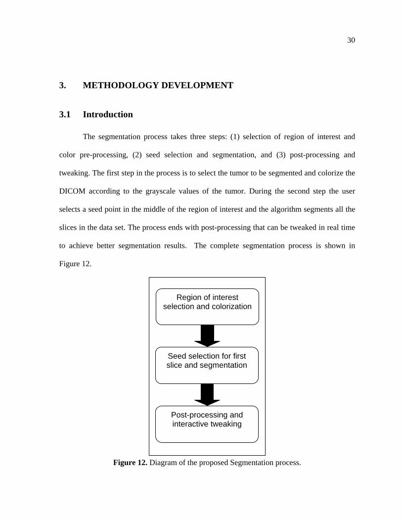
3. METHODOLOGY DEVELOPMENT 30
3.1 Introduction 30
3.2 Color Pre-Processing 31
3.3 Segmentation 36
3.4 Post-Processing 40
4. USER INTERFACE DESIGN AND DEVELOPMENT 42
4.1 Features 43
5. RESULTS AND DISCUSSION 52
5.1 Information of Test Datasets 52
5.2 Evaluation of the Segmentation Method 53
5.3 Hardware 56
5.4 Color segmentation 56
5.4.1 Summary of results 65
5.4.2 Sensitivity 66
iv
5.5 Grayscale segmentation 68
5.5.1 Algorithm 68
5.5.2 Results 69
5.5.3 Limitations of Grayscale Thresholding 74
5.6 Comparison to other segmentation methods 74
5.7 Timing 77
5.8 Limitations of the segmentation algorithm using color pre-processing 78
6. CONCLUSIONS 80
6.1 Summary of conclusions 80
6.2 Future work 81
ACKNOWLEDGMENTS 83
REFERENCES 84
v
LIST OF FIGURES
Figure 1. Representation of 2D Slices forming a 3D Set. 2
Figure 2. DICOM file structure. 3
Figure 3. Three different tumors of the abdomen: homogeneous tumor (a),
tumor with fuzzy edges (b), heterogeneous tumor with calcification (c). 5
Figure 4. Grayscale and color DICOM file. 6
Figure 5. Windowing Process. HU values to pixel intensities. 7
Figure 6. Examples of image processing techniques. 8
Figure 7. Examples of first digital images. 9
Figure 8. Electromagnetic Spectrum. 19
Figure 9. Representation of the RGB color space. 21
Figure 10. Colorization technique by Welsh. 23
Figure 11. Medical Imaging Software packages. 28
Figure 12. Diagram of the proposed Segmentation process. 30
Figure 13. Selection of the region of interest that delineates the tumor. 31
Figure 14. Colorization scheme used to assign RGB values to the pixels.
The minimum HU value is set to red and the maximum HU value is set to blue. 32
Figure 15. Sample results from the color pre-processing method. 34
Figure 16. Same slice with different HU ranges show different tissues. Figure (a)
shows the tumor in blue, Figure (b) shows the tumor in green and many tissues
are set to black. Tumor is delineated in yellow. 35
Figure 17. Example of seed placement on the colorized image. 36
vi
Figure 18. Segmentation results for test case #7 using the same threshold but
different HU ranges. Figure a shows more selected pixels. Yellow line
delineates the tumor. 39
Figure 19. Example of a 5x5 structuring element. 40
Figure 20. Segmentation without post process (left) and with post processing (right). 41
Figure 21. Programmatic building blocks for Medical Imaging Application. 42
Figure 22. User interface available features: visualization, segmentation,
and collaboration. 43
Figure 23. Application Interface highlighting the 2D tab that allows the user to see
DICOM files on the left side of the frame. 44
Figure 24. Example of a DICOM file windowed and not windowed on the Medical
Interface. Windowing and slice scrollbars are highlighted in red. 45
Figure 25. Examples of Sagitall and Coronal View of DICOM sets. Features of 2D
tab such as pseudocoloring and views are highlighted in red. 45
Figure 26. LUT pseudocoloring of DICOM images in the 2D tab. 47
Figure 27. Example of Volume Rendering of set of DICOM files. 48
Figure 28. Windowed Volume of DICOM dataset. 49
Figure 29. Volume Renders with different Pseudocoloring applied. 49
Figure 30. Segmentation tab that shows different color ranges. (a) Shows most tissues
because the color range is big (b) shows the tumor and some other tissues
because the color range is small. 50
Figure 31. Example of Sockets Tab. 51
vii
Figure 32. False positive results of the two best test runs for each test case. 56
Figure 33. False negative results of the two best test runs for each test case. 57
Figure 34. Test case #1 threshold 0.06. Yellow outlines tumor, red is the
segmentation results by the algorithm. 59
Figure 35. Test Case #3 Threshold 45%. The seed is placed on only part of the
tumor and the algorithm selects both regions. 60
Figure 36. Test Case #5. The tumor edges have similar densities to the healthy
tissues surrounding the tumors. 61
Figure 37. Test case #5 threshold 0.2. Yellow outlines the approximate tumor,
red is the actual segmentation by the algorithm. 62
Figure 38. Test Case #6 Threshold 45%. Yellow outlines the approximate tumor,
red is the actual segmentation by the algorithm. 63
Figure 39. Test Case #7 Threshold 40%. Yellow outlines the approximate tumor,
red is the actual segmentation by the algorithm. 64
Figure 40. Test Case #10 Threshold 28%. Yellow outlines the approximate tumor,
red is the actual segmentation by the algorithm. 65
Figure 41. Standard deviation for each test case over the different test runs. 67
Figure 42. Segmentation Results for Grayscale algorithm. Yellow outlines the
approximate tumor, red is the actual segmentation by the algorithm. 70
Figure 43. Grayscale Segmentation Results Case 6. Yellow outlines the
approximate tumor, red is the actual segmentation by the algorithm. 72
viii
Figure 44. Test case #7. Yellow outlines the approximate tumor, red is the actual
segmentation by the algorithm. 73
Figure 45. False Positive results for three segmentation methods: Grayscale (gray),
Color (red), Probabilistic (green). 75
Figure 46. False Negative results for three segmentation methods: Grayscale (gray),
Color (red), Probabilistic (green). 75
ix
LIST OF TABLES
Table 1. Body Tissues and corresponding HU Values. 6
Table 2. Tumor Test Cases description. 53
Table 3. FP and FN Results for all the test runs. 55
Table 4. Results of the segmentation with color pre-processing . 58
Table 5. Standard deviation results for each of the parameters and the for each
of the test runs. 66
Table 6. Grayscale Accuracy Results. 69
Table 7. Comparison between grayscale and segmentation with color pre-processing . 76
Table 8. Segmentation Times per Test Case. 78
x
ABSTRACT
In the last few decades the medical imaging field has grown considerably, and new
techniques such as computerized axial tomography (CAT) and Magnetic Resonance Imaging
(MRI) are able to obtain medical images in noninvasive ways. These new technologies have
opened the medical field, offering opportunities to improve patient diagnosis, education and
training, treatment monitoring, and surgery planning. One of these opportunities is in the
tumor segmentation field.
Tumor segmentation is the process of virtually extracting the tumor from the healthy
tissues of the body by computer algorithms. This is a complex process since tumors have
different shapes, sizes, tissue densities, and locations. The algorithms that have been
developed cannot take into account all these variations and higher accuracy is achieved with
specialized methods that generally work with specific types of tissue data.
In this thesis a color pre-processing method for segmentation is presented. Most
tumor segmentation methods are based on grayscale values of the medical images. The
method proposed in this thesis adds color information to the original values of the image. The
user selects the region of interest (ROI), usually the tumor, from the grayscale medical image
and from this initial selection, the image is mapped into a colored space. Tissue densities that
are part of the tumor are assigned an RGB component and any tissues outside the tumor are
set to black. The user can tweak the color ranges in real time to achieve better results, in
cases where the tumor pixels are non-homogenous in terms of intensity. The user then places
a seed in the center of the tumor and begins segmentation. A pixel in the image is segmented
as part of the tumor if it’s within an initial 10% threshold. This threshold is determined if the
xi
seed is within the average RGB values of the tumor, and within the search region. The search
region is calculated by growing or shrinking the previous region using the information or
previous segmented regions of the set of slices. The method automatically segments all the
slices on the set from the inputs of the first slice. All through the segmentation process the
user can tweak different parameters and visualize the segmentation results in real time.
The method was run on ten test cases several runs were performed for each test cases.
10 out of the 20 test runs gave false positives of 25% or less, and 10 out of the 20 test runs
gave false negatives of 25% or less. Using only grayscale thresholding methods the results
for the same test cases show a false positive of up to 52% on the easy cases and up to 284%
on the difficult cases, and false negatives of up to 14% on the easy cases and up to 99% on
the difficult cases. While the results of the grayscale and color pre-processing methods on
easy cases were similar, the results of color pre-processing were much better on difficult
cases, thus supporting the claim that adding color to medical images for segmentation can
significantly improve accuracy of tumor segmentation.
1
1. INTRODUCTION
The role of digital images and digital imaging processing in various technical fields
has increased considerably in the past few decades. Significant applications of digital image
processing are evident in astronomy, manufacturing, and law enforcement to name a few. In
astronomy, digital images of star constellations are obtained by capturing the gamma-ray
band; in product manufacturing, higher-energy X-rays digital images of circuit boards can be
examined for flaws; and in law enforcement, digital images of license plates can be read to
monitor traffic [1].
Another field that has successfully implemented digital image processing is medicine;
the increase in computational technology has expanded the role of digital images and digital
image processing in medicine. Medical image data such as CT/MR images can be analyzed
and visualized as two-dimensional and three-dimensional data using computers, minimizing
the need of invasive surgery [1]. It is now possible to store, process, and visualize vast
amounts of medical information. Medical images provide tools for diagnosis, treatment, and
education of pathologies and create opportunities that can benefit health care [2].
1.1 Medical Imaging
X-rays are one of the oldest techniques used for medical imaging. X-rays have a
vacuum tube with a cathode and anode. The cathode is heated causing free electrons to be
released toward the anode. When the electrons strike a nucleus, energy is released in the form
of X-ray radiation, this energy is used by X-ray sensitive film to produce an image [1].
2
Today, two popular processes to obtain medical digital images in noninvasive ways
are computerized axial tomography (CAT), also called computerized tomography (CT) for
short, and Magnetic Resonance Imaging (MRI). In 1972, Sir Geoffrey Hounsfield introduced
the first CT machine. CT technology uses X-rays to obtain images. The first scanner took
several hours to obtain the raw data and several days to reconstruct the data into an image.
Currently, the latest machines are capable of collecting four images in 350 ms and
constructing a 512x512 image in less than a second [3].
In 1977, Paul Lauterbur and Peter Mansfield introduced the first MRI machine. MRI
technology uses the electro-magnetic energy in the radio frequency (RF) to obtain medical
images. Different parts of the body will emit different variations in the RF range and using
these different RF ranges the MRI image is formed [4].
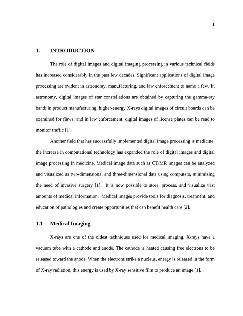
MRI and CT scanners produce a series of two-dimensional (2D) slices that can be
combined to form a three-dimensional (3D) representation of the data, as shown in Figure 1.
Figure 1. Representation of 2D Slices forming a 3D Set.
In the last decade medical images are being stored using the Digital Imaging and
Communications in Medicine (DICOM) standard instead of the traditional 2D printed films.
3
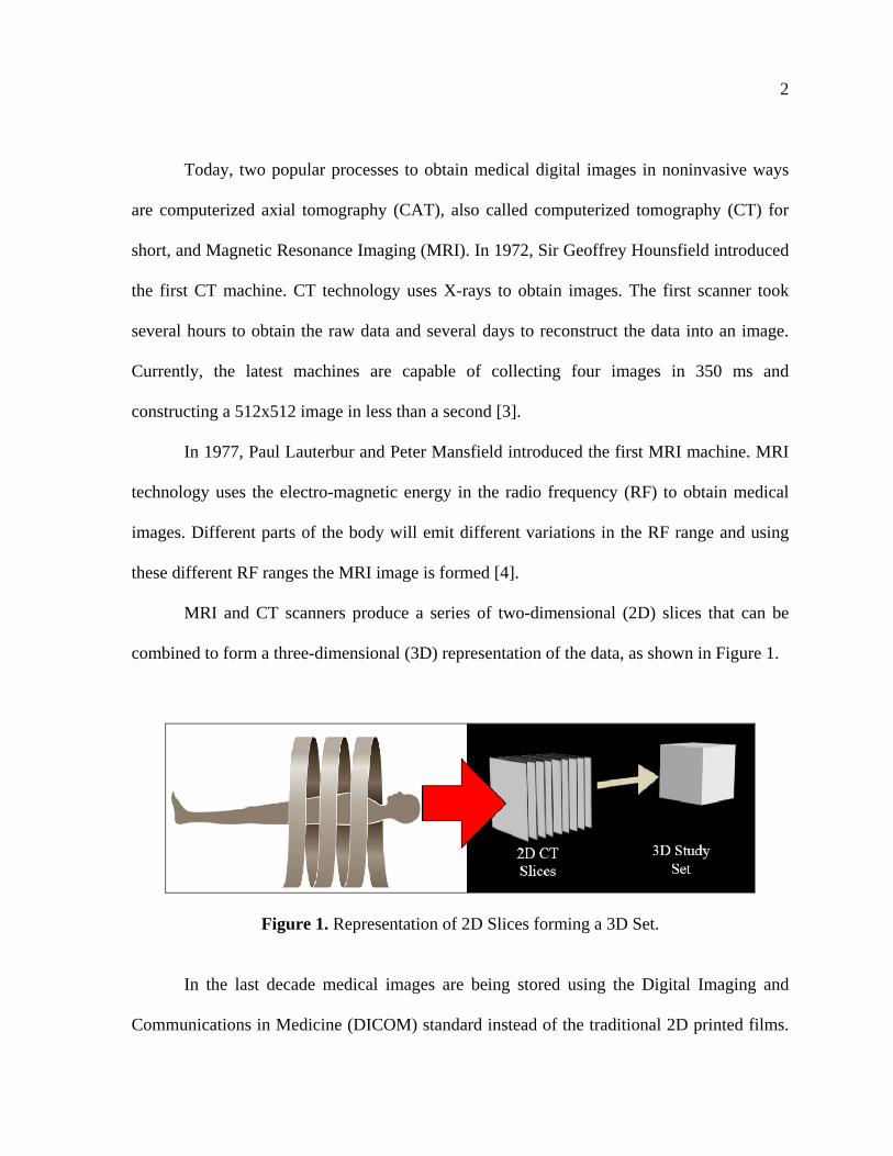
The DICOM standard was developed between the American College of Radiology (ACR)
and the National Electrical Manufacturers Association (NEMA) in 1993. The DICOM
standard is structured as a multi-part document that facilitates the evolution of the standard
since parts can be removed or added easily. These multi-parts or elements are composed of
attributes, shown in Figure 2, such as a tag that works as the identifier, the length of the data,
and a value field with the data [5]. This allows for a DICOM file to not only have image data
but other types of data such as the patient name, age, ID, etc. Having the same format for a
single file with different types of information for all patients facilitates the ease of data
transfer and the implementation of software for digital processing and analysis.
Figure 2. DICOM file structure.
4
Software packages such as Volview and OsiriX can be used to visualize these
medical data by parsing the DICOM files into image and information data. The parsing
process is the process of interpreting the data from the DICOM files into data usable for
visualization and analysis. These packages offer different tools to manipulate the medical
data and assess different information. Some of these tools include rendering a 3D volume
from 2D images, clipping, and constructing animations. One of these tools is segmentation,
one of the most difficult tasks in image processing.
1.2 Medical Image Segmentation
Delineation of regions of interest from an image is referred to as image segmentation.
In Figure 3, the tumor on the image is circled in red; this area should be segmented from the
image. Medical image segmentation plays a role in applications such as diagnosis,
localization of pathologies, treatment, and education. Different segmentation algorithms have
been developed for different objects of interest for example the segmentation of bone is
different from the segmentation of tumor. General methods exist that can be used for
different data, but higher accuracy is achieved with specialized methods. Currently there is
not a single segmentation method that can be used in every medical image and still produce
successful results. Figure 3 shows abdomen tumors of different patients; even from the same
part of the body the tumors to be segmented have different shapes, sizes, intensity values, and
locations. The algorithms try to take into account some of these variations; however they
have difficulties achieving successful results. Tumors of different parts of the body add
another layer of difficulty to the segmentation process, and current methods are not able to
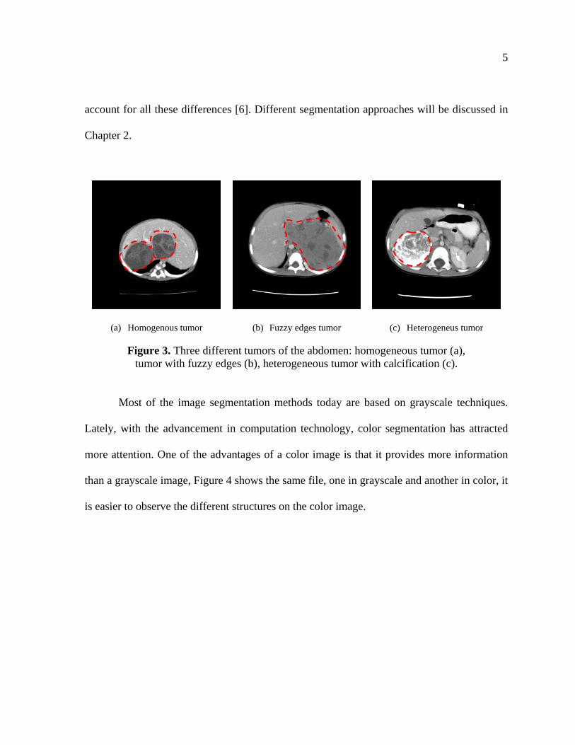
5
account for all these differences [6]. Different segmentation approaches will be discussed in
Chapter 2.
(a) Homogenous tumor (b) Fuzzy edges tumor (c) Heterogeneus tumor
Figure 3. Three different tumors of the abdomen: homogeneous tumor (a), tumor with fuzzy edges (b), heterogeneous tumor with calcification (c).
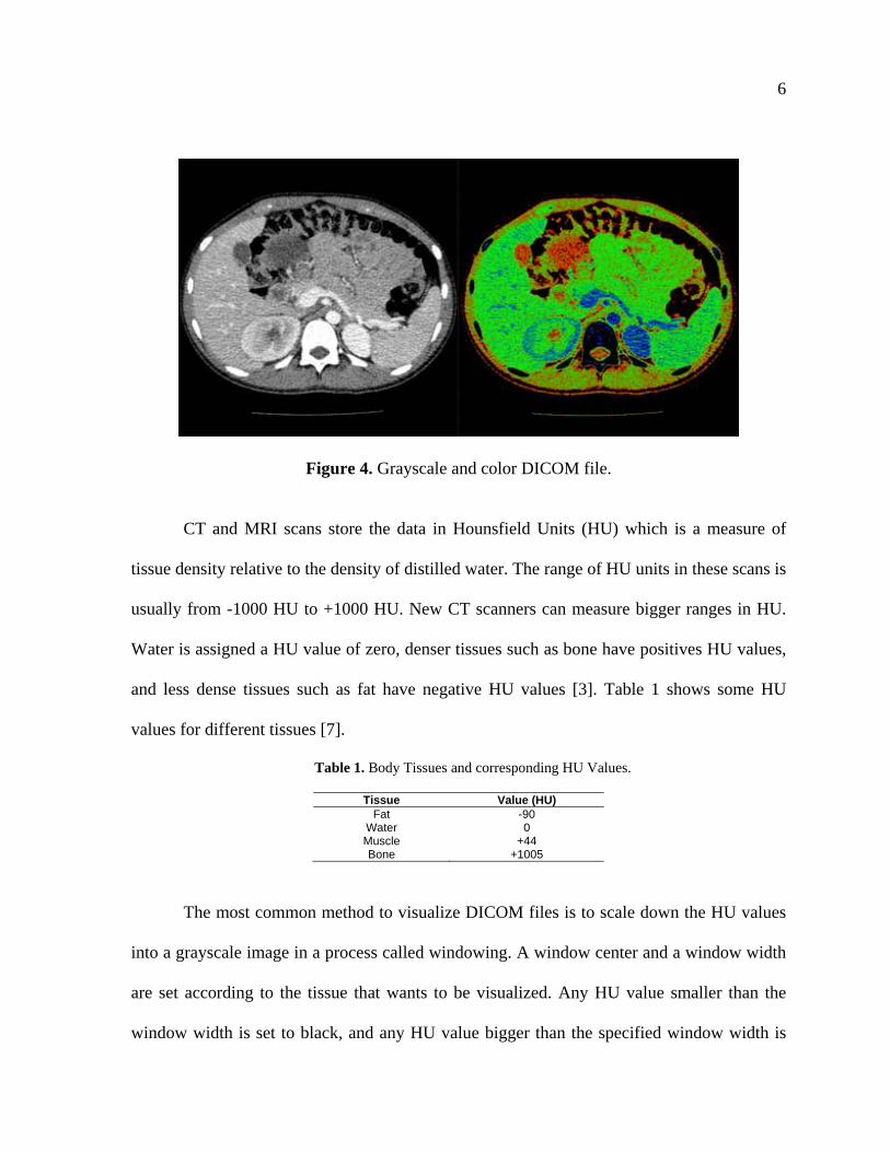
Most of the image segmentation methods today are based on grayscale techniques.
Lately, with the advancement in computation technology, color segmentation has attracted
more attention. One of the advantages of a color image is that it provides more information
than a grayscale image, Figure 4 shows the same file, one in grayscale and another in color, it
is easier to observe the different structures on the color image.
6
Figure 4. Grayscale and color DICOM file.
CT and MRI scans store the data in Hounsfield Units (HU) which is a measure of
tissue density relative to the density of distilled water. The range of HU units in these scans is
usually from -1000 HU to +1000 HU. New CT scanners can measure bigger ranges in HU.
Water is assigned a HU value of zero, denser tissues such as bone have positives HU values,
and less dense tissues such as fat have negative HU values [3]. Table 1 shows some HU
values for different tissues [7].
Table 1. Body Tissues and corresponding HU Values.
Tissue Value (HU) Fat -90
Water 0 Muscle +44 Bone +1005
The most common method to visualize DICOM files is to scale down the HU values
into a grayscale image in a process called windowing. A window center and a window width
are set according to the tissue that wants to be visualized. Any HU value smaller than the
window width is set to black, and any HU value bigger than the specified window width is
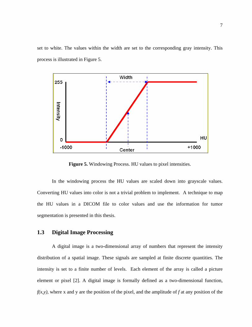
7
set to white. The values within the width are set to the corresponding gray intensity. This
process is illustrated in Figure 5.
Figure 5. Windowing Process. HU values to pixel intensities.
In the windowing process the HU values are scaled down into grayscale values.
Converting HU values into color is not a trivial problem to implement. A technique to map
the HU values in a DICOM file to color values and use the information for tumor
segmentation is presented in this thesis.
1.3 Digital Image Processing
A digital image is a two-dimensional array of numbers that represent the intensity
distribution of a spatial image. These signals are sampled at finite discrete quantities. The
intensity is set to a finite number of levels. Each element of the array is called a picture
element or pixel [2]. A digital image is formally defined as a two-dimensional function,
f(x,y), where x and y are the position of the pixel, and the amplitude of f at any position of the
8
pixel is called the intensity or gray level of the image at that point. Digital imaging
processing is the manipulation of digital images to produce different output images, two
common digital image processes are blurring and sharpening. Blurring is used to remove
noise and detail from an image; sharpening on the other hand improves the image contrast
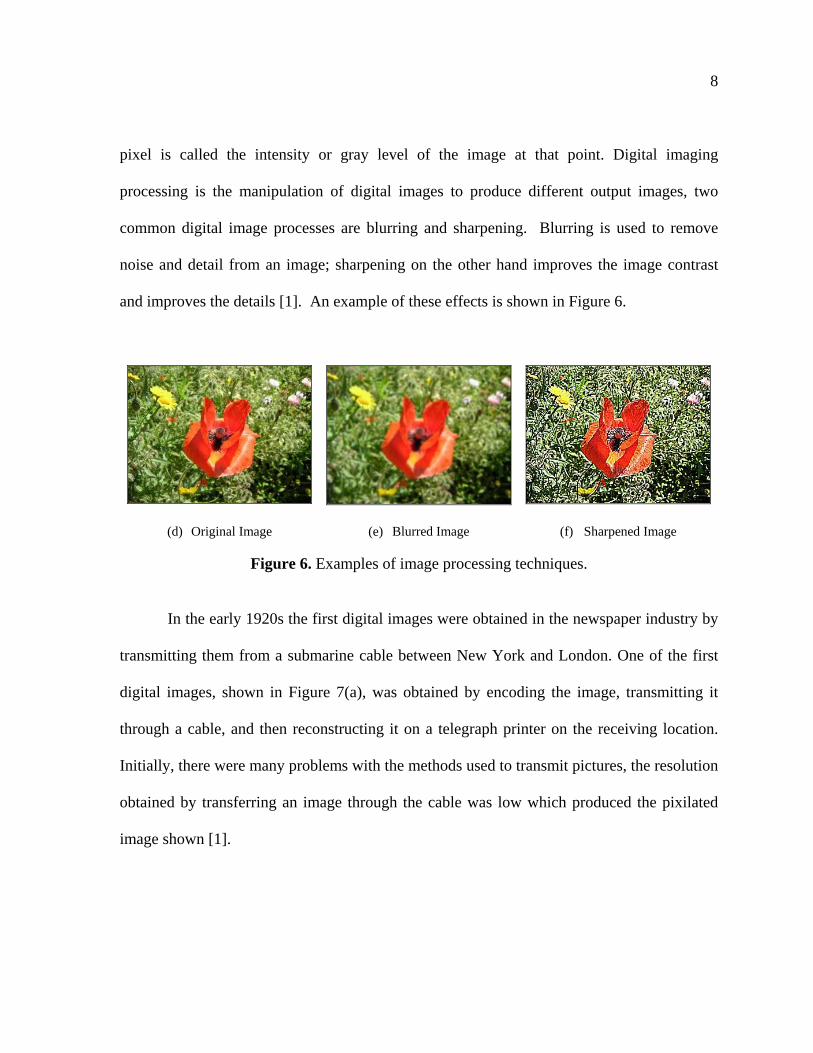
and improves the details [1]. An example of these effects is shown in Figure 6.
(d) Original Image (e) Blurred Image (f) Sharpened Image
Figure 6. Examples of image processing techniques.
In the early 1920s the first digital images were obtained in the newspaper industry by
transmitting them from a submarine cable between New York and London. One of the first
digital images, shown in Figure 7(a), was obtained by encoding the image, transmitting it
through a cable, and then reconstructing it on a telegraph printer on the receiving location.
Initially, there were many problems with the methods used to transmit pictures, the resolution
obtained by transferring an image through the cable was low which produced the pixilated
image shown [1].
9
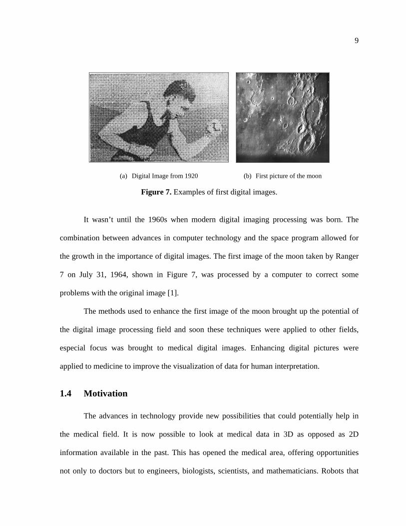
(a) Digital Image from 1920 (b) First picture of the moon
Figure 7. Examples of first digital images.
It wasn’t until the 1960s when modern digital imaging processing was born. The
combination between advances in computer technology and the space program allowed for
the growth in the importance of digital images. The first image of the moon taken by Ranger
7 on July 31, 1964, shown in Figure 7, was processed by a computer to correct some
problems with the original image [1].
The methods used to enhance the first image of the moon brought up the potential of
the digital image processing field and soon these techniques were applied to other fields,
especial focus was brought to medical digital images. Enhancing digital pictures were
applied to medicine to improve the visualization of data for human interpretation.
1.4 Motivation
The advances in technology provide new possibilities that could potentially help in
the medical field. It is now possible to look at medical data in 3D as opposed as 2D
information available in the past. This has opened the medical area, offering opportunities
not only to doctors but to engineers, biologists, scientists, and mathematicians. Robots that
10
assist in surgery such as the da Vinci surgical system [8], assisted surgery from different
locations [9], and virtual reality [10] to visualize data are now a reality. Perhaps in the future
robots will be able to perform surgeries automatically, and computers will be able to predict
how a tumor will develop.
The tumor segmentation problem is an interesting one, it is fundamental for many
other future applications in medicine and to this date there is no unique solution. Providing a
set of tools for doctors to visualize tumors could beneficiate patients in many ways. In order
to create these tools not only the segmentation results for the tumor extraction must be
accurate but also these tools must be easy to use.
This thesis will address both areas of the problem. It will present a technique to
colorize the grayscale data in DICOM files, and then use this color information to segment
tumors. It will also provide software that allows the user to implement the segmentation
techniques, and other visualization tools for medical data, in a fast, easy, and intuitive
manner. This framework took advantage of 2D textures to allow users to manipulate
segmentation data quickly, textures communicate with the graphics hardware in an efficient
way to allow for fast and real time visualization of the results.
1.5 Thesis Organization
This thesis is divided into six chapters. The second chapter presents the background
information with the literature review on medical segmentation, colorization of HU data,
color segmentation, medical data user interfaces, and graphical hardware used with medical
data. The methodology used for the segmentation algorithms and the development of the user

11
interface are found in chapters three and four. Chapter five presents results from the
segmentation algorithms as well as the discussion of these results. And conclusions and
future work are presented in chapter six.
12
2. LITERATURE REVIEW
2.1 Segmentation
The goal of segmentation varies from case to case. In some instances, the objective is
to divide the image into groups, like gray matter, white matter, and fluids in the brain. In
other cases, the purpose is to extract a single structure from the image such as a tumor in a
CT scan. And some other applications have for their objective to classify the image into
anatomical features such as bones, muscles, and vessels [2].
As mentioned in the introduction chapter, due to the variations in medical information
there is not a general segmentation technique that can produce accurate results for every case
and every goal. The literature review showed a vast and varied number of medical image
segmentation methods. Most of the medical imaging segmentation techniques are based on
grayscale methods [2, 11-14].
Segmentation methods discussed in this chapter can be categorized into at least one of
the following groups [11]: (1) thresholding approaches (2) region growing approaches, (3)
classifiers, (4) clustering approaches, (5) Markov random field (MRF) models, (6) artificial
neural networks, (7) deformable models, and (8) atlas-guided approaches.
Reference [12] categorizes segmentation into two broad categories: (1) single 2D or
3D image segmentation and (2) Multi-spectral image segmentation, in which segmentation is
performed on a set of images that have different grayscale values.
Taking into account the framework of this thesis, the grayscale segmentation
techniques are classified into three groups: (1) classical approaches, such as thresholding and
13
region growing, (2) advanced approaches such as probability approaches, deformable
models, fuzzy logic, and (4) hybrid approaches. These methods are covered in detail in the
following sections.
2.1.1 Classical Approaches
In general, classical methods only use the information that is provided by the image
[15]. Classical methods include thresholding techniques, clustering techniques and region
growing techniques [2].
Thresholding techniques are characterized by using pixel intensity levels. A pixel is
selected if its density is equal or less to the density set by the user [13]. If the density level of
the object is significantly different from the density of the background images, then
thresholding becomes a very affective and simple method for segmentation [16].
Thresholding has several limitations, classical thresholding techniques do not take into
account spatial pixel relations or any other information besides grayscale density thus
thresholding becomes sensitive to noise or non homogenous images, which are common
occurrence in medical images [11].
Region growing is a technique in which the user places a pixel in the image, called a
seed, and the region grows by adding neighboring pixels if they are within certain threshold
of the current region [17]. One of the limitations of this classical technique is that it requires
user input for the initial seed point. Another limitation is that selecting a pixel based on the
threshold of the region makes the technique susceptible to noise. Methods that combine
classical region grow with more approaches can overcome some of these limitations [18-19].
14
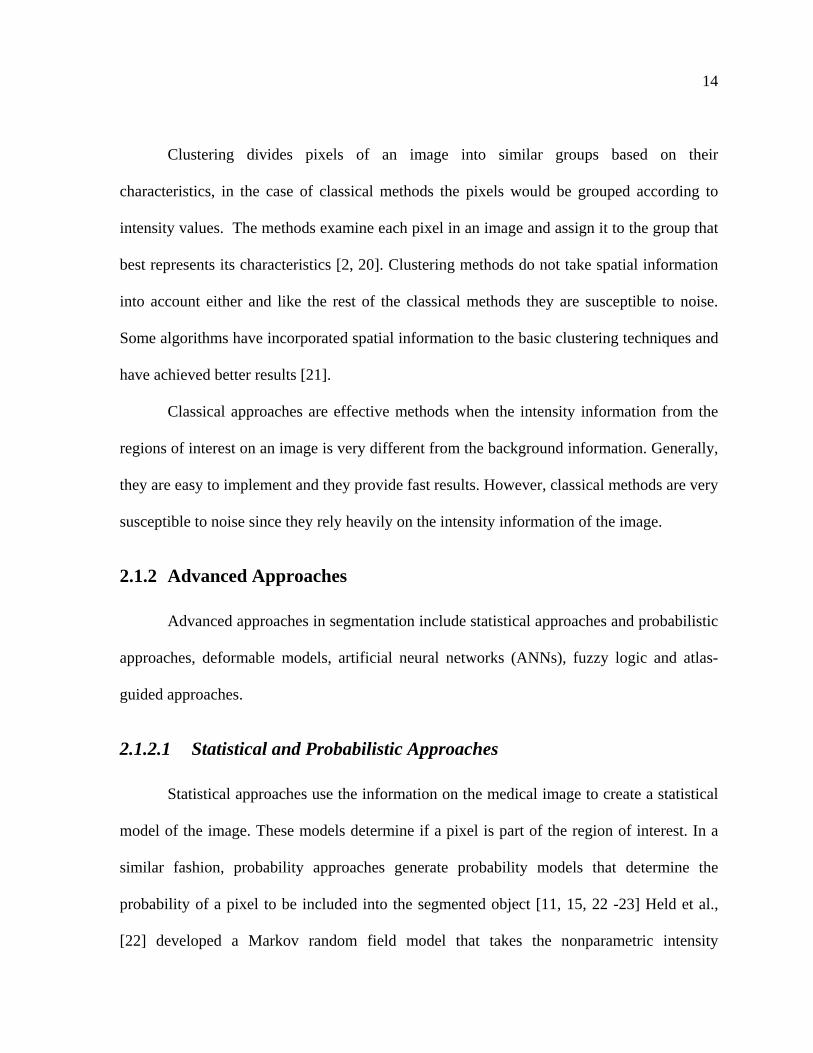
Clustering divides pixels of an image into similar groups based on their
characteristics, in the case of classical methods the pixels would be grouped according to
intensity values. The methods examine each pixel in an image and assign it to the group that
best represents its characteristics [2, 20]. Clustering methods do not take spatial information
into account either and like the rest of the classical methods they are susceptible to noise.
Some algorithms have incorporated spatial information to the basic clustering techniques and
have achieved better results [21].
Classical approaches are effective methods when the intensity information from the
regions of interest on an image is very different from the background information. Generally,
they are easy to implement and they provide fast results. However, classical methods are very
susceptible to noise since they rely heavily on the intensity information of the image.
2.1.2 Advanced Approaches
Advanced approaches in segmentation include statistical approaches and probabilistic
approaches, deformable models, artificial neural networks (ANNs), fuzzy logic and atlas-
guided approaches.
2.1.2.1 Statistical and Probabilistic Approaches
Statistical approaches use the information on the medical image to create a statistical
model of the image. These models determine if a pixel is part of the region of interest. In a
similar fashion, probability approaches generate probability models that determine the
probability of a pixel to be included into the segmented object [11, 15, 22 -23] Held et al.,
[22] developed a Markov random field model that takes the nonparametric intensity
15
distributions and the neighborhood correlations of the pixels to create the segmentation
algorithm.
Vincken et al., [24] uses a probabilistic segmentation, in which the child pixels of the
3D image, called child voxels, are linked to more than one parent voxel. This linkage
determines the final volume.
Statistical and probability methods tend to yield accurate results. However, these
methods initially need to prepare models before the segmentation which causes heavy
burdens on computer and time resources [15].
2.1.2.2 Deformable Models
Deformable models delineate a region of interest by using parametric curves or
surfaces [11]. These curves or surfaces can move under the influence of internal forces and
external forces. The internal forces, the curve or surface in itself are designed to keep the
model smooth during the deformation. The external forces, computed from the image data
are used to move the model toward the region of interest [25]. By combining internal and
external forces deformable models tend to be robust models.
Kaus et al [26] propose a deformable model method to segment myocardium in 3D
MRI. The deformable model is represented by a triangular mesh. After initially positioning
the mesh, the model adapts by carrying out surface detection in each triangle of the mesh and
by reconfiguration of the mesh vertices. The internal forces of this method restrict the
flexibility of the segmentation by maintaining the configuration of an initial mesh. And the
external forces drive the mesh towards the surface points.
16
One of the limitations of deformable models is that they require initial interaction
from the user to set up the model and the parameters [11]. Another limitation is that
deformable models are used for highly specific cases [27].
2.1.2.3 Artificial Neural Networks (ANNs)
ANNs are nodes that simulate a biological neural system. Each node has a weight
associated to it that determines how the pixels should be classified [28]. Huang et al [29]
developed a model that uses Neural Networks to contour breast tumors. In their method a
hidden learning algorithm assigns weights to the neurons based on texture features of the
image. An input vector is compared with all weight vectors and it is matched with the best
neuron which corresponds to an associated output. The neural network was used as a filter
for subsequent segmentation algorithms.
One of the advantages of learning algorithms is that they can be applied to a wide
range of problems. One of the limitations of learning algorithms is that they have to be
trained, if the training set is not large enough errors occur, the same happens if it is over
trained. Another limitation is that ANN is a black-box problem, given an input, the learning
algorithm gives an output, however the details of the operations are unknown: how reliable
the output is, and how was the decision reached [30].
2.1.2.4 Fuzzy Logic
Fuzzy logic is a theory that represents the vagueness of everyday life, for example
when cooking concepts like add hot water, put salt to taste are not crisp instructions, they
allow certain liberties. Images are by nature fuzzy and fuzzy logic methods use the vagueness
17
concept to perform segmentation. Fuzzy connectedness methods [31-32] are clustering
methods in which every pair of pixels are assigned an affinity to each other according to
different parameters such as spatial relations and intensity levels. This affinity defines the
fuzzy connected project. Moonis et al [33] used fuzzy logic to segment brain tumors. To
determine the affinity they used the training facility 3DVIEWNIX. Using this system they
painted the tumor and edema for one patient by using a paint brush, from this one patient the
affinity values were calculated and used for all the subsequent studies. For each study they
first selected a general rectangular region that contained the tumor, this region was used to
decrease processing as the algorithm ignored anything outside of this region. Then they
planted seed points on the region of interest and their fuzzy-connectedness algorithm
delineated the actual tumor.
One of the limitations of fuzzy logic approaches is that the user has to choose input
parameters and the affinity relations which requires a lot more initial interaction than with
other methods.
2.1.2.5 Atlas-guided approaches
Atlas-guided approaches create a model by compiling information on the anatomy of
the region of interest. This model or atlas is used as the reference to segment new images. It
allows for the use of both spatial and intensity information of the image [11, 34]. Lorenzo-
Valdes et al [34] developed a method to segment 3D cardiac images. To construct the general
atlas they manually segmented 18 to 20 cycles of the heart composed of eight to ten slices of
18
14 adults. Using transformation algorithms they created a subject atlas, and then using a
registration method they aligned the general atlas to the subject atlas.
Atlas-guided approaches are very robust if the model and the new images are similar
to the training set of images, but they are not capable of segmenting accurately images that
are varied to the training set. For example if the training set is of the brain the algorithm
would not be able to segment abdomen images.
Advanced methods tend to achieve better results than classical techniques, but they
require more input from the user, and because they have more complex equations they take
more time to implement and to process than classical approaches.
2.1.3 Hybrid Approaches
Many segmentation methods do not fall within a single segmentation group as they
integrate different approaches to overcome limitations and they are classified as hybrid
approaches. Gibout et al [35] combined k-means, a classical clustering approach, and
deformable models to create an algorithm that takes advantage of the speed of classical
approaches and the accuracy of advanced approaches.
Atkins et al [36] developed a method that uses a thresholding approach and
deformable models to segment the brain in MRI. The first step in the algorithm uses
histogram analysis to remove noise, the second stage produces a model to identify regions of
the brain, and the third step locates the boundary of the brain.
Hybrid approaches can complement the weaknesses of the methods to achieve better
segmentation results but one of their limitations is that hybrid approaches tend to be more
19
complex than the approaches which can translate into heavy burdens in computer and time
resources
2.2 Colorization
2.2.1 Color Fundamentals
The color spectrum can be divided into six regions: violet, blue, green, yellow,
orange, and red. These colors do not end abruptly but blend from one color to the next. The
color of an object perceived by humans is determined by the wavelength of the light reflected
from the object. If an object reflects light in all visible wavelengths, the object will be
perceived as white to the observer. But if the object only reflects certain wavelengths the
object will exhibit a specific color. For example, objects that reflect light between
wavelengths of 500 and 570 nm are perceived as having green color. Color light spans the
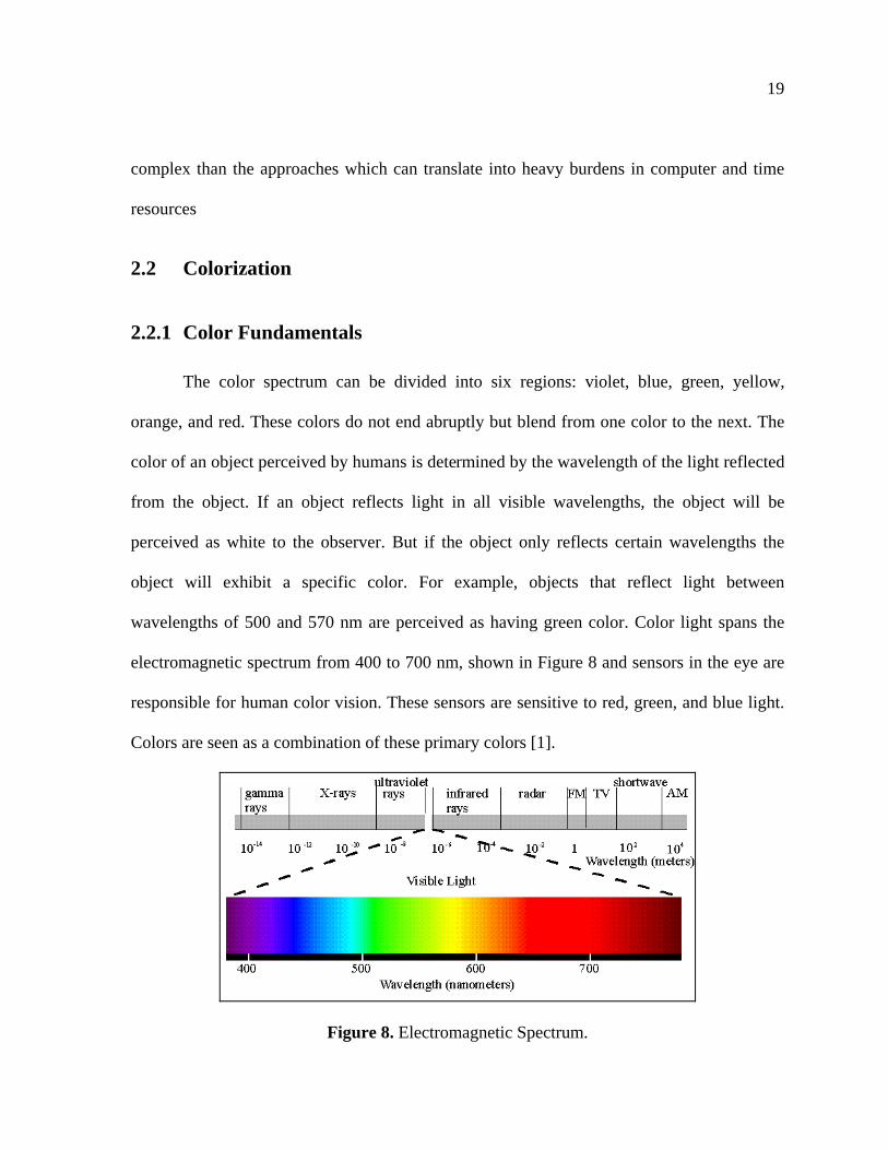
electromagnetic spectrum from 400 to 700 nm, shown in Figure 8 and sensors in the eye are
responsible for human color vision. These sensors are sensitive to red, green, and blue light.
Colors are seen as a combination of these primary colors [1].
Figure 8. Electromagnetic Spectrum.
20
Three characteristics are generally used to describe color: brightness, hue, and
saturation. Brightness is almost impossible to describe and it embodies the achromatic
(without color) notion of light intensity. Hue describes the dominant wavelength in a mixture
of light waves, the dominant color of an object. Saturation describes the amount of white
light mixed with a hue. For example pink, the combination of red and white, is a color less
saturated than red [1].
Color models or color spaces, specify the colors in a standard way by using a
coordinate system and a subspace in which each color is represented by a single point [1].
The most common color spaces used in image processing methods are RGB and HIS.
The red, green, and blue (RGB) color space can be represented in a 3D cube, shown
in Figure 9, color can be represented by the combination of the reg, green, and blue colors.
This color space is commonly used for television systems and pictures of digital cameras
[37].
21
Figure 9. Representation of the RGB color space.
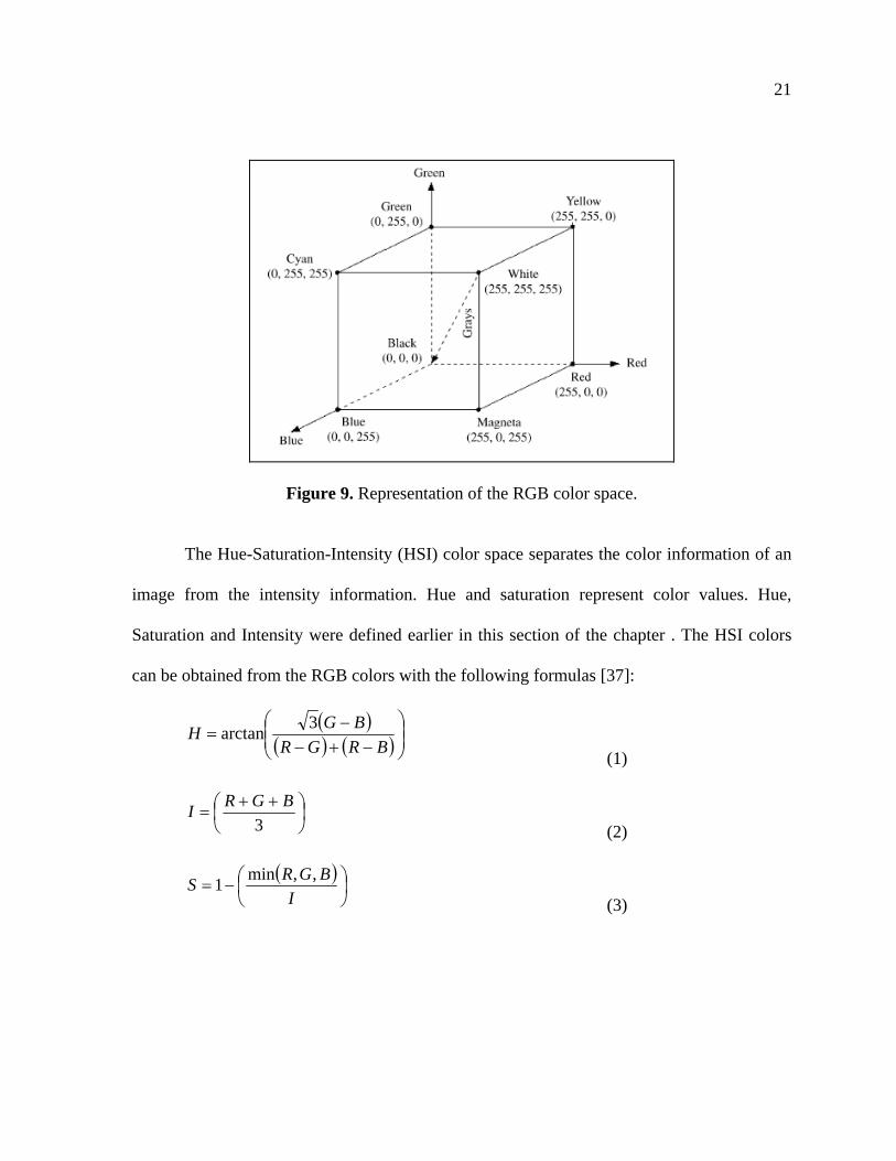
The Hue-Saturation-Intensity (HSI) color space separates the color information of an
image from the intensity information. Hue and saturation represent color values. Hue,
Saturation and Intensity were defined earlier in this section of the chapter . The HSI colors
can be obtained from the RGB colors with the following formulas [37]:
BRGR
BGH
3arctan
(1)
3
BGRI
(2)
I
BGRS
,,min1
(3)
22
2.2.2 General Colorization Concepts
Colorization is the process of adding color to a grayscale image by the use of a
computer. It is a difficult and time-consuming process, and automatic algorithms are not
accurate enough and existing methods usually require extensive user input [38]. The
problem of colorization is assigning three-dimensional information to a pixel from the
original one-dimensional image. Colorization in RGB will add color channels to the image
from 1 channel to 3 channels which will increase the possible number of colors from 256 to
16 million. With the current colorization techniques there is not a unique solution that will
specify which of those new 16 million colors will best represent the image, and thus so far
colorization is very dependent on user input [39-40].
Transfer functions and lookup tables are two concepts used widely in the colorization
field. Transfer functions are functions that take the corresponding information of the image to
obtain new color information and assign this information to the data being visualized, thus
every colorization method uses a transfer function. Lookup Tables (LUT) give a color output
from a grayscale input. Every lookup table is obtained from a transfer function. Some
colorization techniques are focused on the final colorized image, while others are focused on
creating transfer functions that can be applied to the same type data [41]. Most transfer
functions are obtained through a “trial and error” method. In which the user modifies the
initial parameter until a good visualization is achieved [42].
23
2.2.3 Colorization Techniques
Some methods ask the user to use a color palette and insert colors to the grayscale
image [38, 40, 43]. For example, Levin et al [38] use a method in which the user colors a
selected number of pixels in certain regions of the image and the algorithm propagates the
colors in the image. The premise is that neighboring pixels that have similar intensities
should have similar colors. One of the advantages of this method is that the user input is
minimal and the results are accurate. However the time can be significant, at least 15 seconds
per image, medical data consists of sets of hundreds of images that would take a lot of time
to colorize. This method only presented images that had no noise; medical data is usually
noisy so the method could have very different results.
Figure 10. Colorization technique by Welsh.
Other methods use a source image to produce the colors [44]. Welsh et al [39]
colorize an image by transferring color from a color image to a destination grayscale image
without the need for the user to select and apply individual colors to the target image, as
shown in Figure 10. A subset of pixels of the color image is used as a sample. Then each of
the pixels in the target grayscale image is matched to the color pixels by using statistics. In
addition, this method can also use swatches to be used as the color source. These swatches
24
work the same way as the color image source, it creates a subset sample. A limitation to this
method is that there needs to be a source image to provide the subset sample, and this image
has to be close in content to the target image. Because of the variation in medical images it
may not be possible to find two source images close enough to the destination image.
Chen et al [45] propose a method in which first the source image is segmented into
objects. Each object is colorized using Welsh et al [39] method and then the objects are
grouped together to form the final image. The presented method only shows images without
noise.
Takahiko et al [46] developed a method that colorizes an image by adding initial
color seeds to the image and the colors propagate by minimizing the color difference among
4-connected pixels. This algorithm is very fast it only takes a few seconds to colorize a
256x256 pixel image. However the final results are not accurate. In addition it requires the
user to pick colors and plant seeds to the source image.
2.2.4 Medical Image Colorization Techniques
As mentioned earlier CT and MRI scans do not contain color information but rather
HU values that can be windowed for visualization. In order to apply color to medical data
pseudocoloring methods are used.
Pseudocoloring is a common technique for adding colors to medical images. One of
the simplest techniques in pseudocoloring is to slice the image into intensity planes, and
assign a color to each plane. This method applies color to the image linearly [1].
25
Tzeng et al [47] implements a method to create a color transfer function by having the
user paint a few slices of the volume data set. The user paints the regions of interest in one
color, and the background data in another color. The voxels are classified by artificial neural
network segmentation approach. This method only works for 3D data.
Silverstein et al [48] developed an algorithm to colorize 3D medical data for human
visualization. The purpose of their work was to realistically colorize medical images to
enhance surgeon’s visual perception. Initially the grayscale volume was divided into main
body tissues such as fat and bone. Each structure was assigned and RGB value as realistically
as possible. These initial values were adjusted by a group of surgeons. The colors between
tissue types were linearly interpolated. From these values luminance was calculated and
added to the data generating perceptual colorization. The user can move the luminance on
the data and change the perception of the colors on the image.
Pelizzari et al [49] developed a technique to render and colorize a volume from
grayscale CT and MRI scans. From a transfer function each voxel in the data is assigned a
weight based on visual attributes like color by using a probabilistic classification of tissue
types. Rays are cast through this weighted voxel from a viewport toward the rendered pixel
that accumulates the visual attributes of the transverse voxels.
2.2.5 Limitations on Colorization Techniques
There are several limitations with the colorization techniques used today. One of the
limitations is that colorization techniques require a lot of user input. Some of them ask for the
user to colorize some images, or pick the correct transfer functions, or add the correct image.
26
Since there is no way to evaluate the output image it is difficult to know if the solution is
accurate. Most of the colorization techniques are focused on creating an image that is close
to reality as perceived by humans. While this can prove an effective tool for diagnostic, it
may not be the only alternative if other goals for colorization want to be achieved like further
computer image processing.
2.3 Color Segmentation Methods
Many of the grayscale segmentation approaches can be extended to color
segmentation. Color segmentation approaches include classical techniques such as
thresholding, clustering, region growing, and advanced approaches such as fuzzy logic, ANN
[37, 50-52].
Some of the classical thresholding techniques separate the color information and
obtain histograms separately on each piece of information [51-52]. Then through a function
they combined the results. Lin et al [53] used the HSI space to segment a road from the
image. They converted the RGB image into HSI space. They calculated a value for each
pixel by using the saturation and the intensity. Pixels were classified according to these
values.
Cheng et al [54] used a fuzzy logic approach that employ the concept of the
homograph to extract homogeneous regions in a color image. In the first stage they used
fuzzy logic to three color components to find threshold for each color component, then the
segmentation results of the three colors were combined to form color clusters. Cheng et al
achieved better results than if thresholding grayscale segmentation was performed.
27
Verikas et al [55] proposed a color segmentation using neural networks. An image
that combined cyan, magenta, and yellow colors was created resulting in an image with nine
color classes. The first stage included four steps created the segmentation. The first step was
a binary decision three, then the second and third step used the neural networks to create
weight vectors. And lastly a fuzzy classification was used to cluster the pixels. The second
stage is a region merging approach to solve over segmentation problems. This method
achieved 98% correct classification.
Cremers et al [56] implemented a hybrid segmentation approach that uses a region-
based level set segmentation method and statistics that can use color information to segment
the object of interest. Given a set of pixel colors at each image location, the minimization of
the cost functions leads to the estimation of the boundary. This algorithm is not accurate in
medical images where intensity characteristics of the region of interest and the background
are similar.
2.3.1 Limitations on Current Color Segmentation Methods
Color segmentation approaches can be more reliable than gray scale segmentation
approaches. However, they also have limitations similar to grayscale approaches. There is
not a robust general algorithm that works for all cases. Picking a color space is difficult as
each color space has advantages and disadvantages. While color images offer additional
more information this can also result in more problems for segmentation algorithms, for
example noise is increased [37, 51-52]. Most of the current color segmentation approaches
deal with images with minimal noise, and sharp contrast between the boundaries, which is

28
not the case for medical images, this can introduce new problems when trying to apply the
current algorithms to medical data.
2.4 Visualization
2.4.1 Current Interfaces
There are several interfaces for medical image visualization. Volview [57] and OsiriX
[58] are two examples. Volview, shown in Figure 11 allows for the visualization of different
medical data such as DICOM files. Tools that are included are volume rendering, cropping,
coloring, segmentation, filtering, and animation. Volview works on Windows XP/Vista.
OsiriX was developed for the Mac OS as an image processing tool for medical data,
is shown in Figure 11. OsiriX allows for the visualization of 2D, 3D, and even medical data
combined with time information to produce videos. Like Volview, OsiriX tools include
volume rendering, coloring, animation, etc.
(a) Volview (b) Osirix
Figure 11. Medical Imaging Software packages.
29
OsiriX and Volview, as long as other medical image visualization software, allow
medical staff to view and manipulate medical data in any personal computer. These tools can
be used to make better assessments about the information. However there are some
limitations with the current software. Osirix and Volview only work on Mac OS and
Windows respectively. They are also complicated pieces of software, as shown in Figure 11,
that could prove difficult to use for novice users.
2.5 Research Issues
Based on the literature review, this thesis is addressing the following research issue:
1) To improve the accuracy and speed of tumor segmentation from medical image data
using color pre-processing and interactive user inputs.
As discussed segmentation methods currently available are still limited in a number
of ways. According to the literature color segmentation improves the results over grayscale
methods, however these segmentation methods have been performed when the initial input
images already have the color information, which is not the case of medical data. Efforts to
add color to medical data have focused on achieving good end visualization results even
using segmentation algorithms to add the right colors to the corresponding tissues. Colorizing
the medical data first and performing segmentation on this new information to provide better
segmentation results is a new concept.
30
3. METHODOLOGY DEVELOPMENT
3.1 Introduction
The segmentation process takes three steps: (1) selection of region of interest and
color pre-processing, (2) seed selection and segmentation, and (3) post-processing and
tweaking. The first step in the process is to select the tumor to be segmented and colorize the
DICOM according to the grayscale values of the tumor. During the second step the user
selects a seed point in the middle of the region of interest and the algorithm segments all the
slices in the data set. The process ends with post-processing that can be tweaked in real time
to achieve better segmentation results. The complete segmentation process is shown in
Figure 12.
Region of interest selection and colorization
Seed selection for first slice and segmentation
Post-processing and interactive tweaking
Figure 12. Diagram of the proposed Segmentation process.
31
3.2 Color Pre-Processing
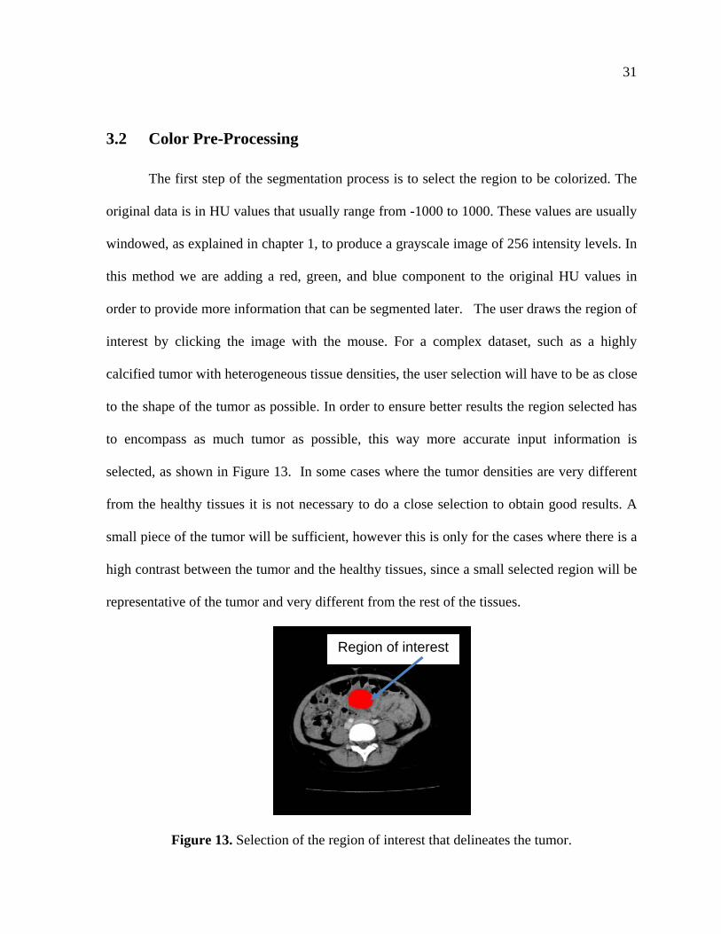
The first step of the segmentation process is to select the region to be colorized. The
original data is in HU values that usually range from -1000 to 1000. These values are usually
windowed, as explained in chapter 1, to produce a grayscale image of 256 intensity levels. In
this method we are adding a red, green, and blue component to the original HU values in
order to provide more information that can be segmented later. The user draws the region of
interest by clicking the image with the mouse. For a complex dataset, such as a highly
calcified tumor with heterogeneous tissue densities, the user selection will have to be as close
to the shape of the tumor as possible. In order to ensure better results the region selected has
to encompass as much tumor as possible, this way more accurate input information is
selected, as shown in Figure 13. In some cases where the tumor densities are very different
from the healthy tissues it is not necessary to do a close selection to obtain good results. A
small piece of the tumor will be sufficient, however this is only for the cases where there is a
high contrast between the tumor and the healthy tissues, since a small selected region will be
representative of the tumor and very different from the rest of the tissues.
Figure 13. Selection of the region of interest that delineates the tumor.
Region of interest
32
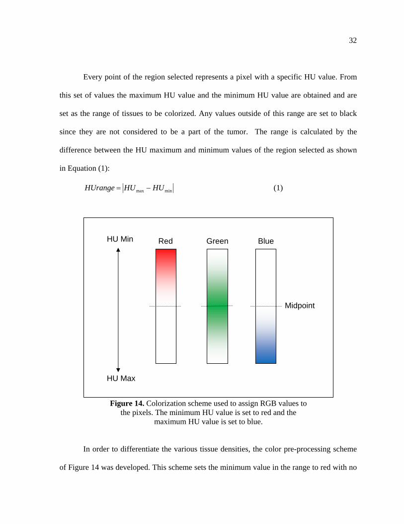
Every point of the region selected represents a pixel with a specific HU value. From
this set of values the maximum HU value and the minimum HU value are obtained and are
set as the range of tissues to be colorized. Any values outside of this range are set to black
since they are not considered to be a part of the tumor. The range is calculated by the
difference between the HU maximum and minimum values of the region selected as shown
in Equation (1):
minmax HUHUHUrange (1)
In order to differentiate the various tissue densities, the color pre-processing scheme
of Figure 14 was developed. This scheme sets the minimum value in the range to red with no
HU Min
HU Max
Midpoint
Red Green Blue
Figure 14. Colorization scheme used to assign RGB values to the pixels. The minimum HU value is set to red and the
maximum HU value is set to blue.
33
blue or green values and the maximum range is set to blue without red or green values, the
rest of the values change from red to blue in a linear fashion, and any values outside the
range are set to black. So any tissues that do not fall in the range to be colorized are not
visible in the image and are ignored in the segmentation process to save processing time. The
goal of this color pre-processing technique is not to provide color to every part of the image
from a grayscale image but rather to highlight tissues of interest with color for effective
segmentation.
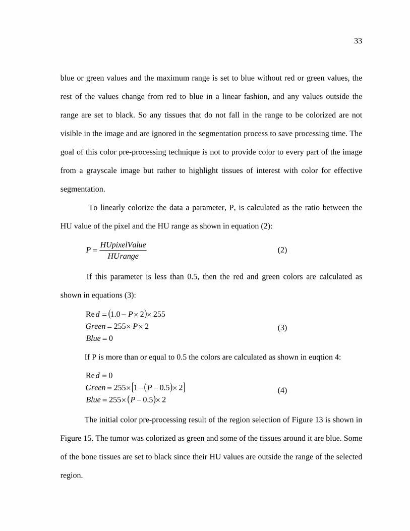
To linearly colorize the data a parameter, P, is calculated as the ratio between the
HU value of the pixel and the HU range as shown in equation (2):
rangeHU
ueHUpixelValP (2)
If this parameter is less than 0.5, then the red and green colors are calculated as
shown in equations (3):
0
2255
25520.1Re
Blue
PGreen
Pd
(3)
If P is more than or equal to 0.5 the colors are calculated as shown in euqtion 4:
25.0255
25.01255
0Re
PBlue
PGreen
d
(4)
The initial color pre-processing result of the region selection of Figure 13 is shown in
Figure 15. The tumor was colorized as green and some of the tissues around it are blue. Some
of the bone tissues are set to black since their HU values are outside the range of the selected
region.
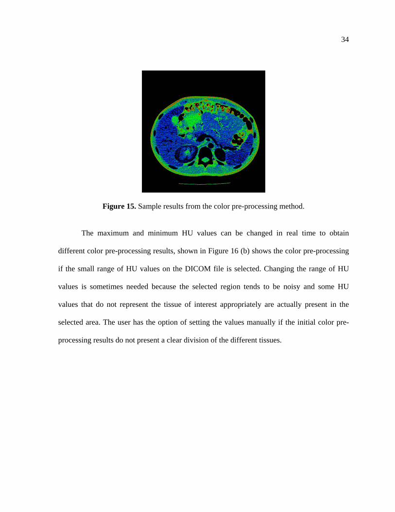
34
Figure 15. Sample results from the color pre-processing method.
The maximum and minimum HU values can be changed in real time to obtain
different color pre-processing results, shown in Figure 16 (b) shows the color pre-processing
if the small range of HU values on the DICOM file is selected. Changing the range of HU
values is sometimes needed because the selected region tends to be noisy and some HU
values that do not represent the tissue of interest appropriately are actually present in the
selected area. The user has the option of setting the values manually if the initial color pre-
processing results do not present a clear division of the different tissues.
35
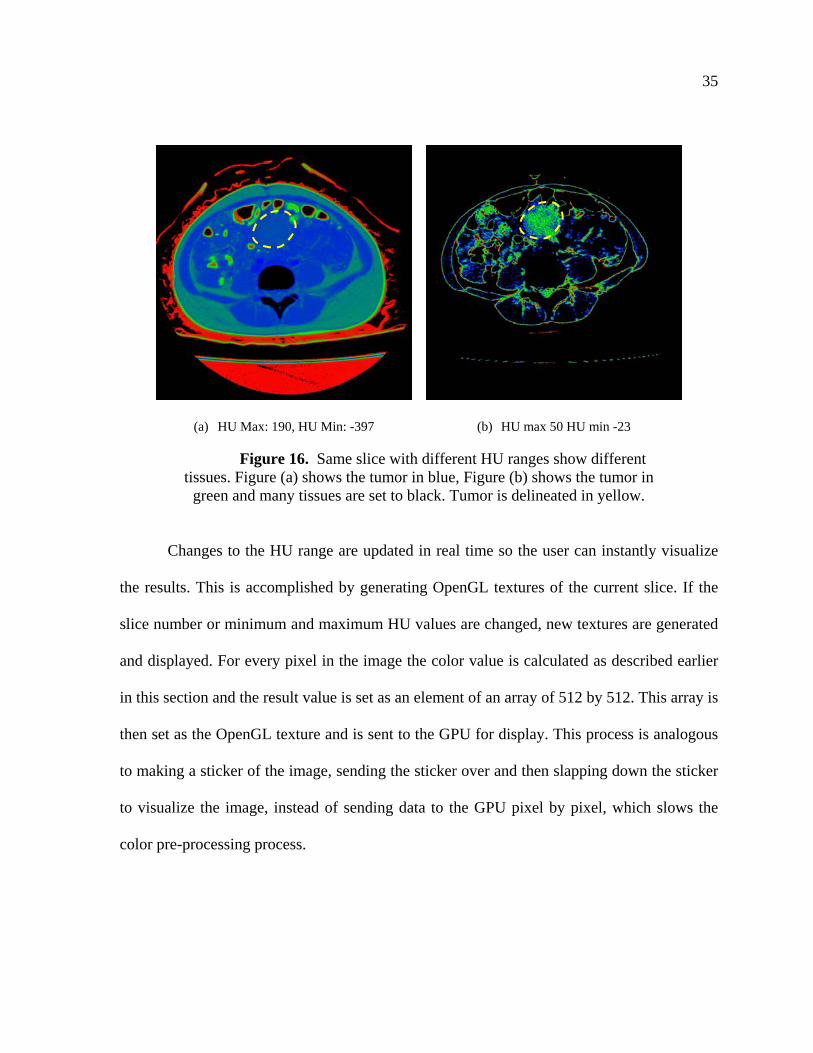
(a) HU Max: 190, HU Min: -397 (b) HU max 50 HU min -23
Figure 16. Same slice with different HU ranges show different tissues. Figure (a) shows the tumor in blue, Figure (b) shows the tumor in
green and many tissues are set to black. Tumor is delineated in yellow.
Changes to the HU range are updated in real time so the user can instantly visualize
the results. This is accomplished by generating OpenGL textures of the current slice. If the
slice number or minimum and maximum HU values are changed, new textures are generated
and displayed. For every pixel in the image the color value is calculated as described earlier
in this section and the result value is set as an element of an array of 512 by 512. This array is
then set as the OpenGL texture and is sent to the GPU for display. This process is analogous
to making a sticker of the image, sending the sticker over and then slapping down the sticker
to visualize the image, instead of sending data to the GPU pixel by pixel, which slows the
color pre-processing process.
36
3.3 Segmentation
Since the work presented is primarily to investigate if color pre-processing can
improve tumor segmentation, a simple segmentation algorithm is used instead of a more
complex segmentation algorithm as a proof of concept. The segmentation algorithm selected
is the basic color thresholding algorithm. Color thresholding uses RGB information instead
of grayscale information. Thresholding techniques are simple methods that perform well
when the tumor and the healthy tissues have high contrast in densities.
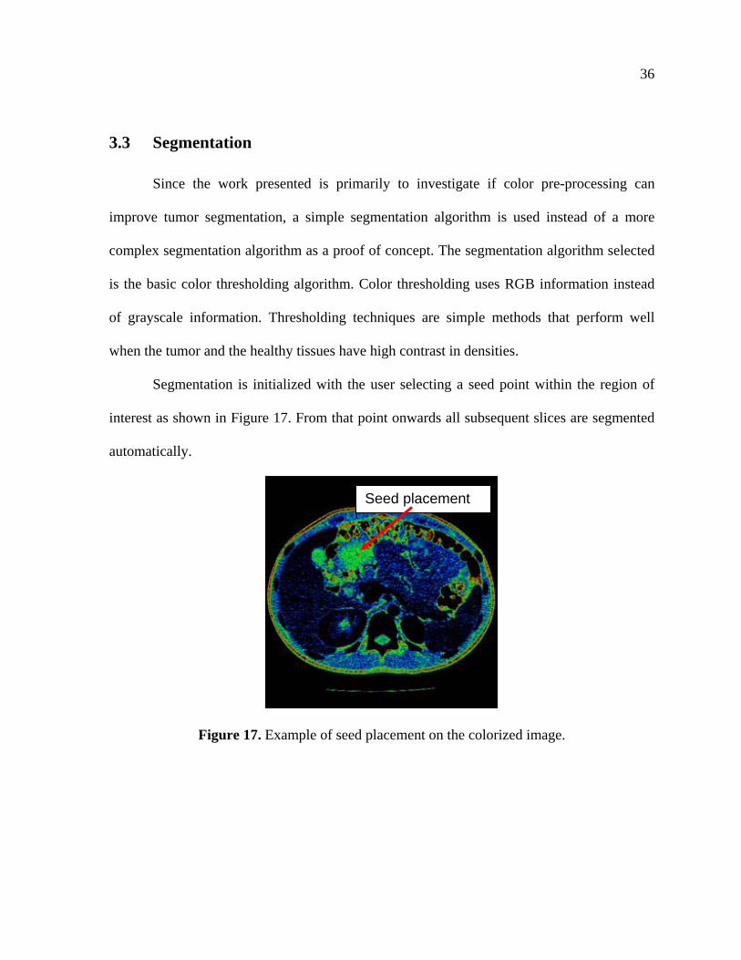
Segmentation is initialized with the user selecting a seed point within the region of
interest as shown in Figure 17. From that point onwards all subsequent slices are segmented
automatically.
Figure 17. Example of seed placement on the colorized image.
Seed placement
37
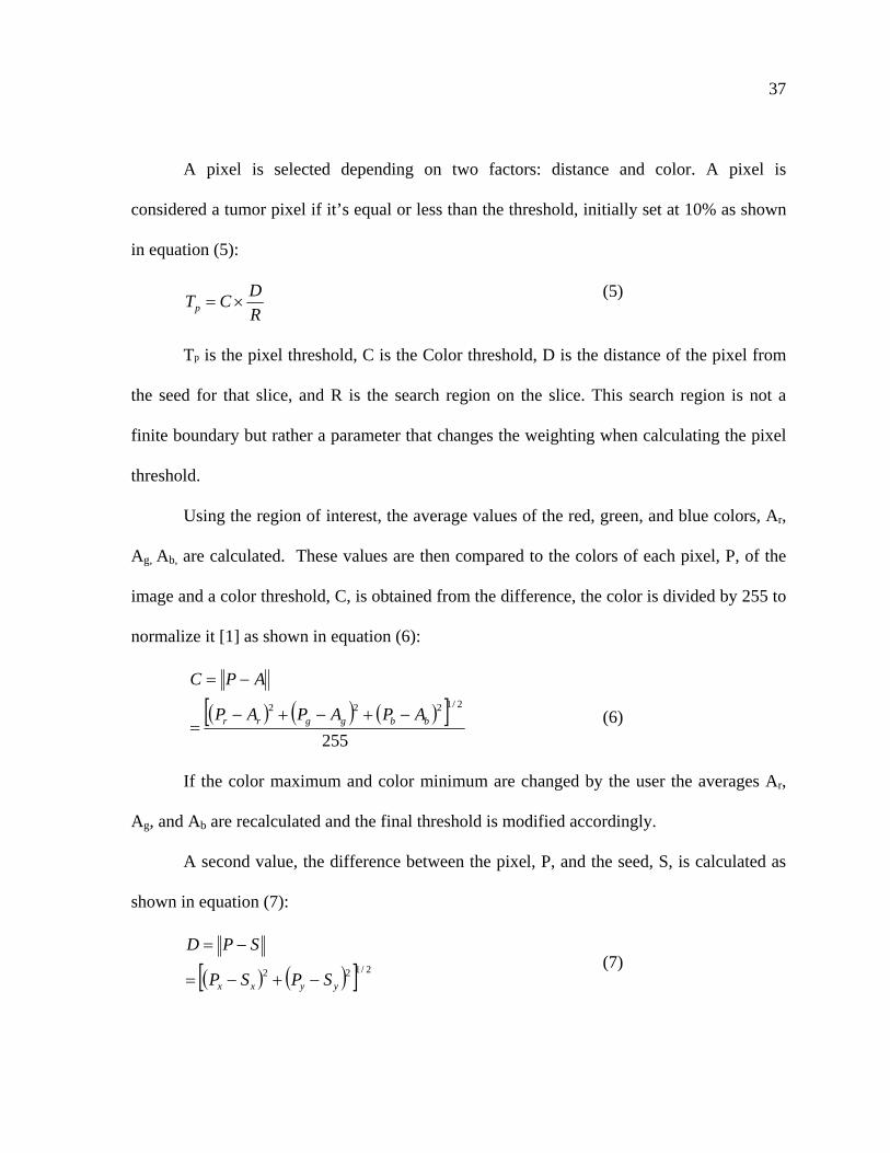
A pixel is selected depending on two factors: distance and color. A pixel is
considered a tumor pixel if it’s equal or less than the threshold, initially set at 10% as shown
in equation (5):
R
DCTp (5)
Tp is the pixel threshold, C is the Color threshold, D is the distance of the pixel from
the seed for that slice, and R is the search region on the slice. This search region is not a
finite boundary but rather a parameter that changes the weighting when calculating the pixel
threshold.
Using the region of interest, the average values of the red, green, and blue colors, Ar,
Ag, Ab, are calculated. These values are then compared to the colors of each pixel, P, of the
image and a color threshold, C, is obtained from the difference, the color is divided by 255 to
normalize it [1] as shown in equation (6):
255
2/1222bbggrr APAPAP
APC
(6)
If the color maximum and color minimum are changed by the user the averages Ar,
Ag, and Ab are recalculated and the final threshold is modified accordingly.
A second value, the difference between the pixel, P, and the seed, S, is calculated as
shown in equation (7):
2/122yyxx SPSP
SPD
(7)
38
For the first slice the seed selected by the user, as shown in Figure 17 in subsequent
slices the seed moves to the center of the previous segmented region. This way the seed will
move with the tumor as the tumor moves.
The search region, R, also grows or shrinks depending on how the tumor grows or
shrinks as shown in equation (8):
pRCR (8)
Rp is search region, of the previous slice. Ci is the percentage of growth or shrinkage
and is defined as shown in equation (9):
6
123 321 iii
i
EEEC (9)
Ei-1 is the growth rate of the tumor in the previous slice and is defined as follows (10):
2-i slice ofregion segmented of Radius
1-i slice ofregion segmented of Radius1 iE (10)
where i is the number of the current slice. For example for the first slice the sum of Ei-1, Ei-2,
and Ei-3 divided by 6 give 1.1 which makes the previous search region, in the case of the first
slice the search region selected by the user to grow by 10%. For slice number 4, E3 is the
segmented region of slice 3 over the segmented region of slice 2, E2 is the segmented region
of slice 2 over the segmented region of slice 1, and E1 is 1.1. This C calculation allows for
the region to grow or shrink depending on how the tumor actually changes.
39
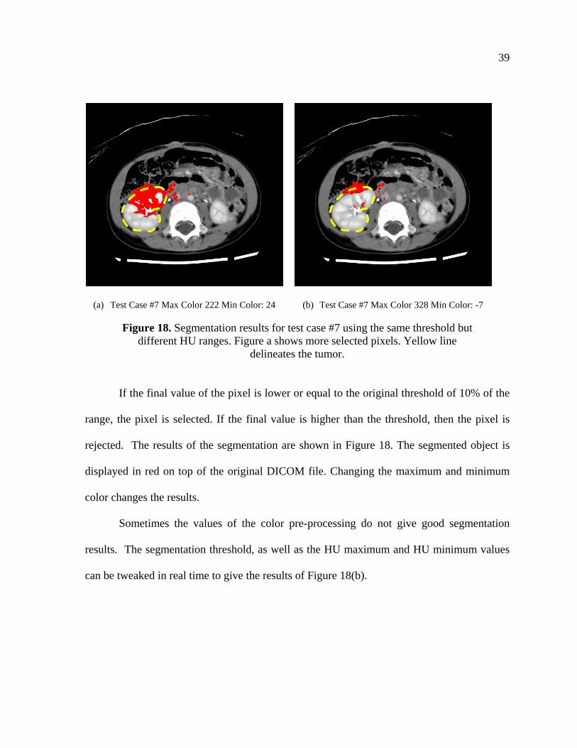
(a) Test Case #7 Max Color 222 Min Color: 24 (b) Test Case #7 Max Color 328 Min Color: -7
Figure 18. Segmentation results for test case #7 using the same threshold but different HU ranges. Figure a shows more selected pixels. Yellow line
delineates the tumor.
If the final value of the pixel is lower or equal to the original threshold of 10% of the
range, the pixel is selected. If the final value is higher than the threshold, then the pixel is
rejected. The results of the segmentation are shown in Figure 18. The segmented object is
displayed in red on top of the original DICOM file. Changing the maximum and minimum
color changes the results.
Sometimes the values of the color pre-processing do not give good segmentation
results. The segmentation threshold, as well as the HU maximum and HU minimum values
can be tweaked in real time to give the results of Figure 18(b).
40
3.4 Post-Processing
Post-processing is the last step of the segmentation process. Morphological operations
on the segmented pixels eliminate some of the stray pixels, or pixels that are not connected to
the segmentation object. This process is performed by eroding and dilating the segmented
pixels.
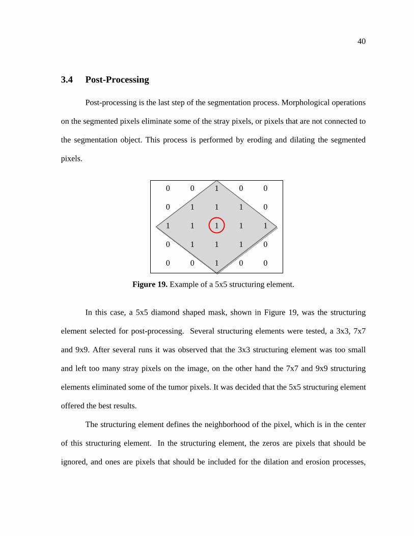
Figure 19. Example of a 5x5 structuring element.
In this case, a 5x5 diamond shaped mask, shown in Figure 19, was the structuring
element selected for post-processing. Several structuring elements were tested, a 3x3, 7x7
and 9x9. After several runs it was observed that the 3x3 structuring element was too small
and left too many stray pixels on the image, on the other hand the 7x7 and 9x9 structuring
elements eliminated some of the tumor pixels. It was decided that the 5x5 structuring element
offered the best results.
The structuring element defines the neighborhood of the pixel, which is in the center
of this structuring element. In the structuring element, the zeros are pixels that should be
ignored, and ones are pixels that should be included for the dilation and erosion processes,
0 0 1 0 0
0 1 1 1 0
1 1 1 1 1
0 1 1 1 0
0 0 1 0 0
41
which are highlighted in gray. This process is repeated for every pixel in the segmented
region.
In erosion, the value of the pixel should be set to the minimum value of any pixels in
the structuring element. Since segmentation has either a selected pixel, of value one, or a
non-selected pixel, of value zero, the final value of the pixel of interest is either zero or one
[59].
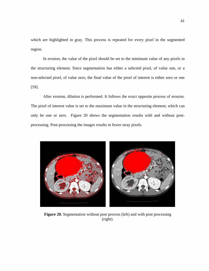
After erosion, dilation is performed. It follows the exact opposite process of erosion.
The pixel of interest value is set to the maximum value in the structuring element, which can
only be one or zero. Figure 20 shows the segmentation results with and without post-
processing. Post-processing the images results in fewer stray pixels.
Figure 20. Segmentation without post process (left) and with post processing (right).
42
4. USER INTERFACE DESIGN AND DEVELOPMENT
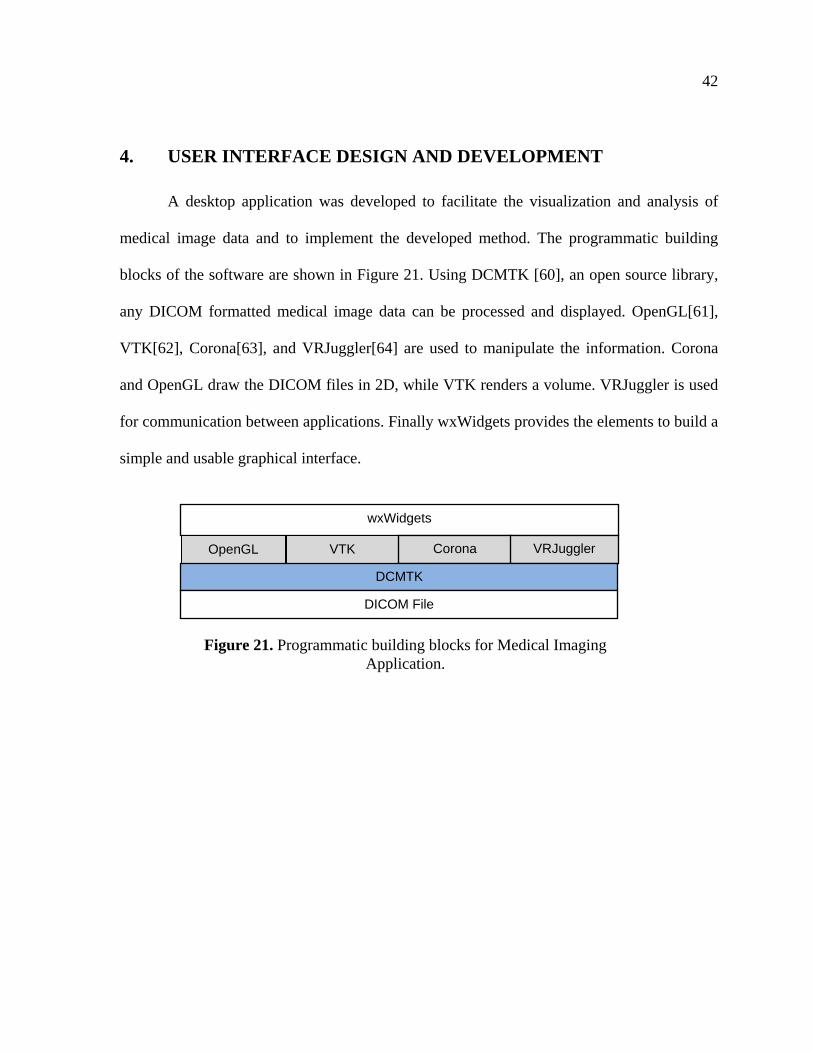
A desktop application was developed to facilitate the visualization and analysis of
medical image data and to implement the developed method. The programmatic building
blocks of the software are shown in Figure 21. Using DCMTK [60], an open source library,
any DICOM formatted medical image data can be processed and displayed. OpenGL[61],
VTK[62], Corona[63], and VRJuggler[64] are used to manipulate the information. Corona
and OpenGL draw the DICOM files in 2D, while VTK renders a volume. VRJuggler is used
for communication between applications. Finally wxWidgets provides the elements to build a
simple and usable graphical interface.
wxWidgets
OpenGL VTK Corona VRJuggler
DCMTK
DICOM File
Figure 21. Programmatic building blocks for Medical Imaging Application.
43
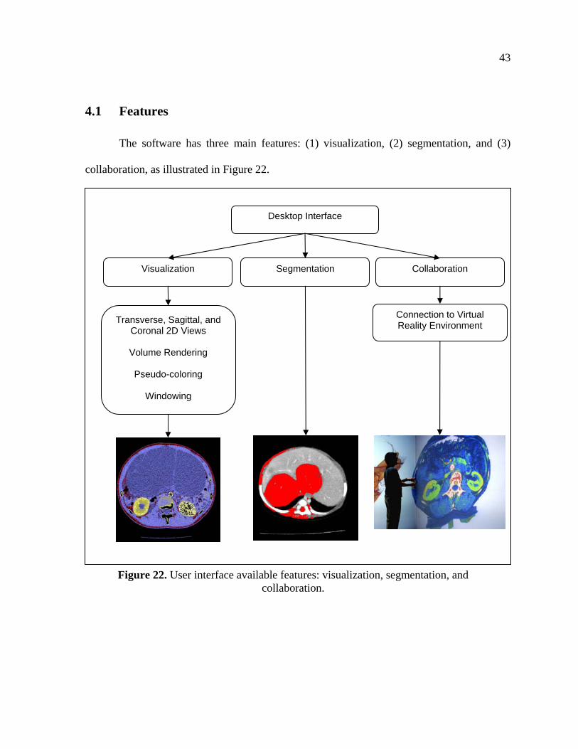
4.1 Features
The software has three main features: (1) visualization, (2) segmentation, and (3)
collaboration, as illustrated in Figure 22.
Desktop Interface
Visualization Segmentation Collaboration
Transverse, Sagittal, and Coronal 2D Views
Volume Rendering
Pseudo-coloring
Windowing
Connection to Virtual Reality Environment
Figure 22. User interface available features: visualization, segmentation, and collaboration.
44
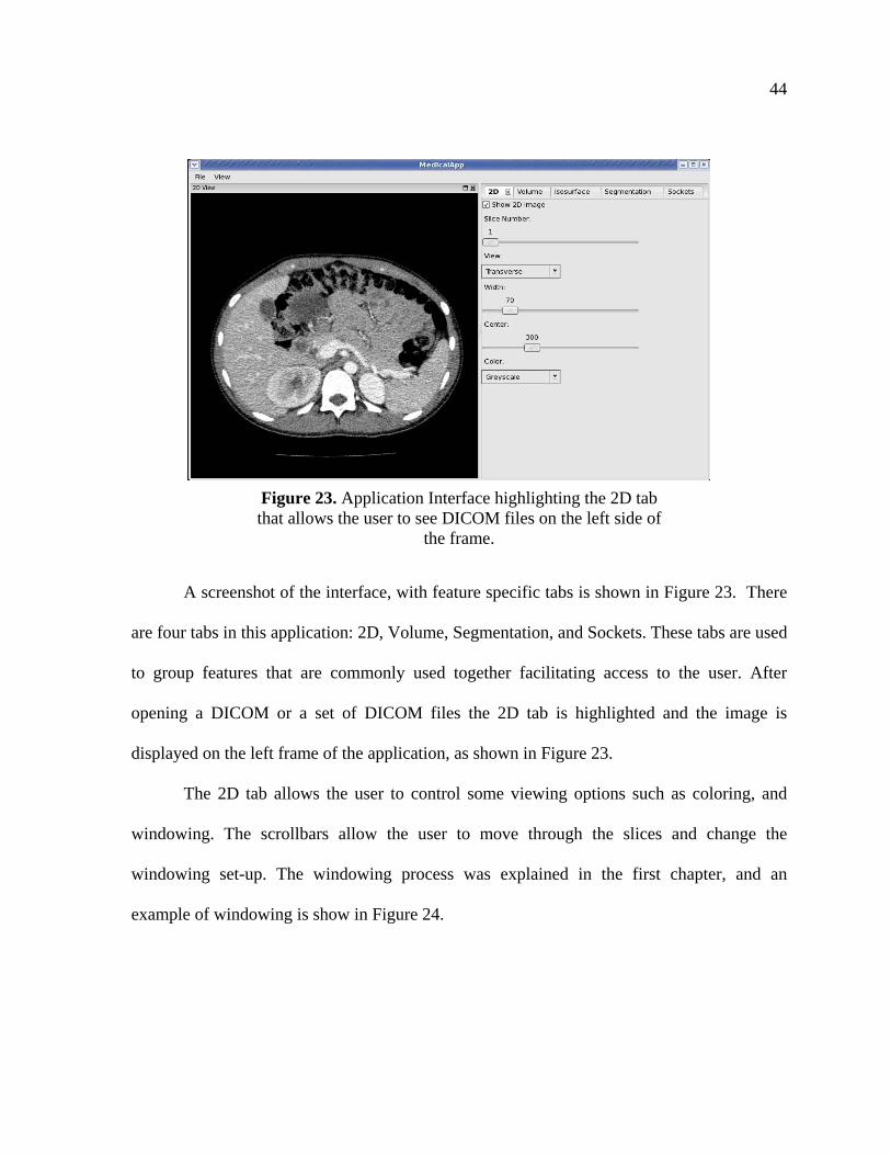
A screenshot of the interface, with feature specific tabs is shown in Figure 23. There
are four tabs in this application: 2D, Volume, Segmentation, and Sockets. These tabs are used
to group features that are commonly used together facilitating access to the user. After
opening a DICOM or a set of DICOM files the 2D tab is highlighted and the image is
displayed on the left frame of the application, as shown in Figure 23.
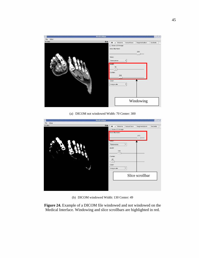
The 2D tab allows the user to control some viewing options such as coloring, and
windowing. The scrollbars allow the user to move through the slices and change the
windowing set-up. The windowing process was explained in the first chapter, and an
example of windowing is show in Figure 24.
Figure 23. Application Interface highlighting the 2D tab that allows the user to see DICOM files on the left side of
the frame.
45
(a) DICOM not windowed Width: 70 Center: 300
(b) DICOM windowed Width: 130 Center: 49
Figure 24. Example of a DICOM file windowed and not windowed on the Medical Interface. Windowing and slice scrollbars are highlighted in red.
Windowing
Slice scrollbar
46
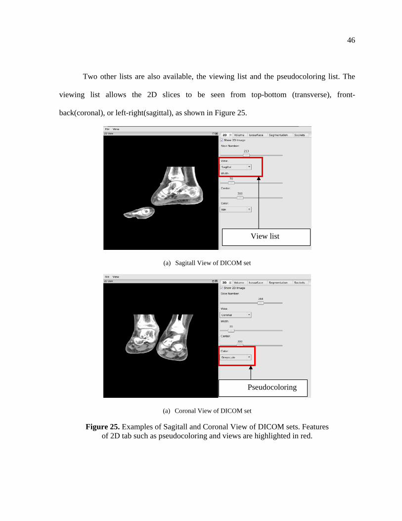
Two other lists are also available, the viewing list and the pseudocoloring list. The
viewing list allows the 2D slices to be seen from top-bottom (transverse), front-
back(coronal), or left-right(sagittal), as shown in Figure 25.
(a) Sagitall View of DICOM set
(a) Coronal View of DICOM set
Figure 25. Examples of Sagitall and Coronal View of DICOM sets. Features of 2D tab such as pseudocoloring and views are highlighted in red.
View list
Pseudocoloring
47
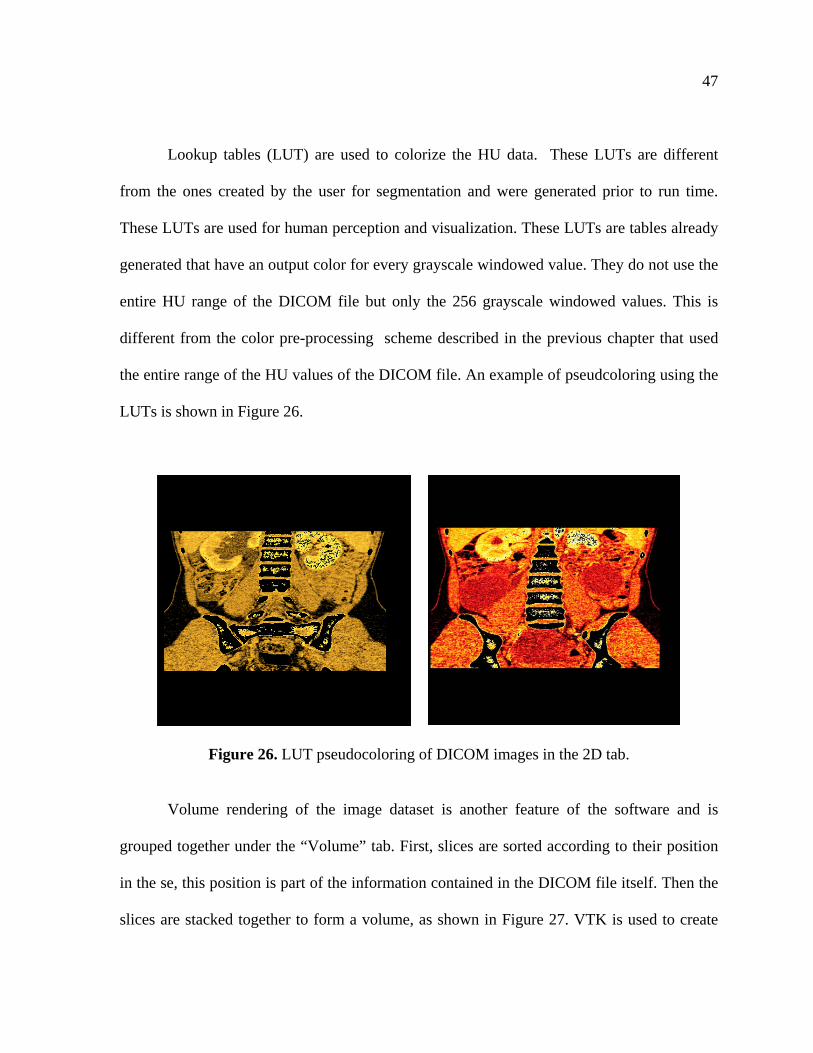
Lookup tables (LUT) are used to colorize the HU data. These LUTs are different
from the ones created by the user for segmentation and were generated prior to run time.
These LUTs are used for human perception and visualization. These LUTs are tables already
generated that have an output color for every grayscale windowed value. They do not use the
entire HU range of the DICOM file but only the 256 grayscale windowed values. This is
different from the color pre-processing scheme described in the previous chapter that used
the entire range of the HU values of the DICOM file. An example of pseudcoloring using the
LUTs is shown in Figure 26.
Figure 26. LUT pseudocoloring of DICOM images in the 2D tab.
Volume rendering of the image dataset is another feature of the software and is
grouped together under the “Volume” tab. First, slices are sorted according to their position
in the se, this position is part of the information contained in the DICOM file itself. Then the
slices are stacked together to form a volume, as shown in Figure 27. VTK is used to create
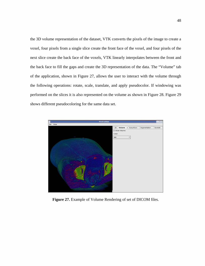
48
the 3D volume representation of the dataset, VTK converts the pixels of the image to create a
voxel, four pixels from a single slice create the front face of the voxel, and four pixels of the
next slice create the back face of the voxels, VTK linearly interpolates between the front and
the back face to fill the gaps and create the 3D representation of the data. The “Volume” tab
of the application, shown in Figure 27, allows the user to interact with the volume through
the following operations: rotate, scale, translate, and apply pseudocolor. If windowing was
performed on the slices it is also represented on the volume as shown in Figure 28. Figure 29
shows different pseudocoloring for the same data set.
Figure 27. Example of Volume Rendering of set of DICOM files.
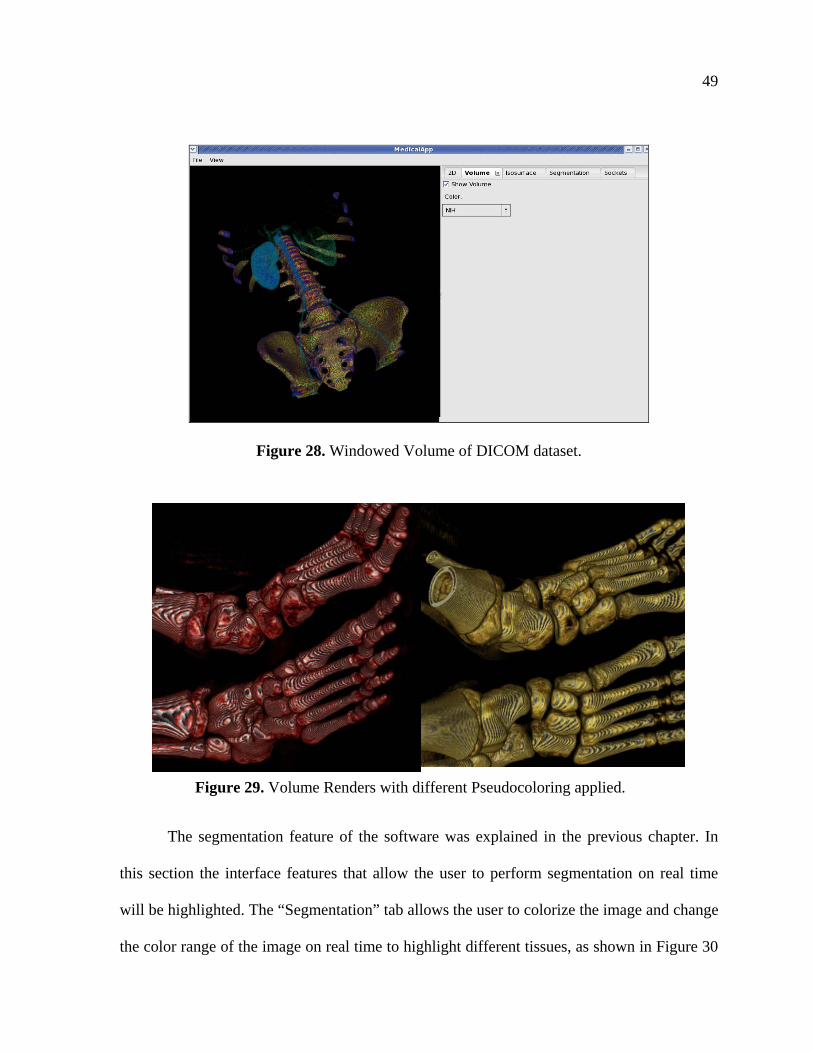
49
Figure 28. Windowed Volume of DICOM dataset.
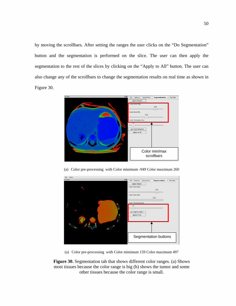
The segmentation feature of the software was explained in the previous chapter. In
this section the interface features that allow the user to perform segmentation on real time
will be highlighted. The “Segmentation” tab allows the user to colorize the image and change
the color range of the image on real time to highlight different tissues, as shown in Figure 30
Figure 29. Volume Renders with different Pseudocoloring applied.
50
by moving the scrollbars. After setting the ranges the user clicks on the “Do Segmentation”
button and the segmentation is performed on the slice. The user can then apply the
segmentation to the rest of the slices by clicking on the “Apply to All” button. The user can
also change any of the scrollbars to change the segmentation results on real time as shown in
Figure 30.
(a) Color pre-processing with Color minimum -949 Color maximum 260
(a) Color pre-processing with Color minimum 159 Color maximum 497
Figure 30. Segmentation tab that shows different color ranges. (a) Shows most tissues because the color range is big (b) shows the tumor and some
other tissues because the color range is small.
Color min/max scrollbars
Segmentation buttons
51
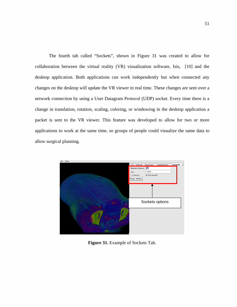
The fourth tab called “Sockets”, shown in Figure 31 was created to allow for
collaboration between the virtual reality (VR) visualization software, Isis, [10] and the
desktop application. Both applications can work independently but when connected any
changes on the desktop will update the VR viewer in real time. These changes are sent over a
network connection by using a User Datagram Protocol (UDP) socket. Every time there is a
change in translation, rotation, scaling, coloring, or windowing in the desktop application a
packet is sent to the VR viewer. This feature was developed to allow for two or more
applications to work at the same time, so groups of people could visualize the same data to
allow surgical planning.
Figure 31. Example of Sockets Tab.
Sockets options
52
5. RESULTS AND DISCUSSION
5.1 Information of Test Datasets
Ten different datasets from seven individuals were used to test the developed color
pre-processing and segmentation method. Test cases #1-3 were a courtesy of Dr G. Miyano
from Juntendo University School of Medicine, Tokyo, Japan. Test case #1 is a Cystic
Teratoma on the left ovary, #2 is an immature Teratoma, and #3 is a MucinousCystadenoma
on the right ovary. Test cases #4-#10 are Neuroblastomas and the courtesy of Dr R.M.
Rangayan from University of Calgary, Alberta, Canada, the different test cases are shown in
Table 2 .
The test cases vary in number of slices and difficulty. There are three levels of
difficulty for these data sets: tumors that have homogeneous densities are classified as a
category A; tumors that have fuzzy edges and have some inhomogeneity in their tissues are
considered of having a category B; tumors that have heterogeneous tissues are of category C.
Some tumors with calcium buildup, which is called calcification, can be considered of
category B or C depending on the degree of the calcification. When a tumor has a lot of
calcification then the tissues densities in the tumors tend to be very different and the
segmentation algorithms cannot easily select all types of densities in the tumor.
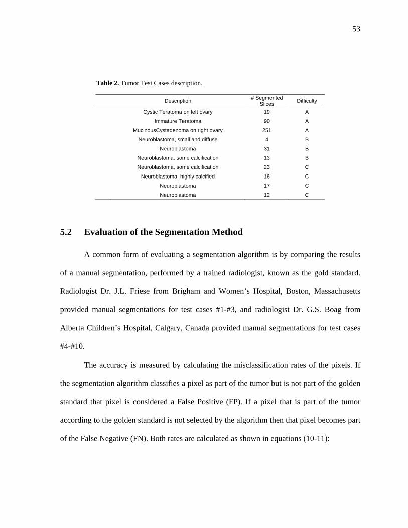
53
Table 2. Tumor Test Cases description.
Description # Segmented
Slices Difficulty
Cystic Teratoma on left ovary 19 A
Immature Teratoma 90 A
MucinousCystadenoma on right ovary 251 A
Neuroblastoma, small and diffuse 4 B
Neuroblastoma 31 B
Neuroblastoma, some calcification 13 B
Neuroblastoma, some calcification 23 C
Neuroblastoma, highly calcified 16 C
Neuroblastoma 17 C
Neuroblastoma 12 C
5.2 Evaluation of the Segmentation Method
A common form of evaluating a segmentation algorithm is by comparing the results
of a manual segmentation, performed by a trained radiologist, known as the gold standard.
Radiologist Dr. J.L. Friese from Brigham and Women’s Hospital, Boston, Massachusetts
provided manual segmentations for test cases #1-#3, and radiologist Dr. G.S. Boag from
Alberta Children’s Hospital, Calgary, Canada provided manual segmentations for test cases
#4-#10.
The accuracy is measured by calculating the misclassification rates of the pixels. If
the segmentation algorithm classifies a pixel as part of the tumor but is not part of the golden
standard that pixel is considered a False Positive (FP). If a pixel that is part of the tumor
according to the golden standard is not selected by the algorithm then that pixel becomes part
of the False Negative (FN). Both rates are calculated as shown in equations (10-11):
54
%100
)(
)(x
RV
RAVAVFP
(10)
%100)(
)()(x
RV
RAVRVFN
(11)
Where V(R) is the volume segmented by the radiologist, the golden standard, and
V(A) is the volume segmented by the algorithm.
The FP rate indicates how the algorithm ignores healthy tissues and only segments
tumor tissues. A low FP rate indicates that the algorithm correctly ignores healthy pixels. The
FN rate indicates how the algorithm correctly classifies tumor pixels. A low FN rate indicates
that the algorithm selects most of the tumor pixels.
The developed color preprocessing and segmentation technique was used on ten test
cases. Five to six test runs were performed for each of the ten test cases and the FP and FN
rates were calculated. The thresholding, HU maximum and HU minimum parameters were
altered, these changes are shown in Table 3. The top two results that gave the lowest FP and
FN values for each test case are discussed in detail in the following section. In addition,
several of the test cases were also segmented using a grayscale thresholding method, this
method was very similar to the color pre-processing method, the only difference is that
instead of comparing the segmentation in the RGB channels the segmentation used only the
original HU values. These additional cases provide a base line to compare how the color
pre-processing, adding three channels of color to a grayscale image improve segmentation.
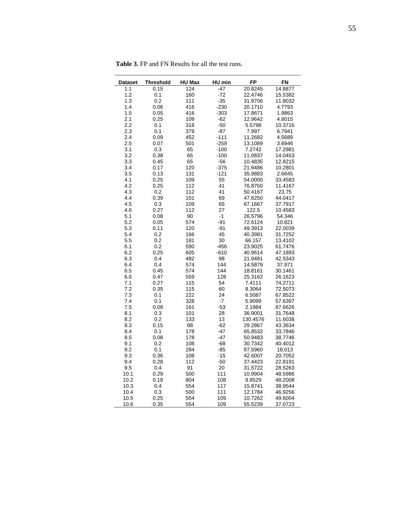
55
Table 3. FP and FN Results for all the test runs.
Dataset Threshold HU Max HU min FP FN 1.1 0.15 124 -47 20.8245 14.8877 1.2 0.1 160 -72 22.4746 15.5382 1.3 0.2 111 -35 31.9706 11.8032 1.4 0.06 416 -230 20.1710 4.7793 1.5 0.05 416 -303 17.8671 1.9863 2.1 0.25 109 -62 12.9642 4.8015 2.2 0.1 318 -50 5.5798 10.3716 2.3 0.1 379 -87 7.997 6.7941 2.4 0.09 452 -111 11.2682 4.5689 2.5 0.07 501 -259 13.1089 3.6946 3.1 0.3 65 -100 7.2742 17.2981 3.2 0.38 65 -100 11.0837 14.0453 3.3 0.45 65 -56 10.4835 12.8215 3.4 0.17 120 -375 21.9486 10.2801 3.5 0.13 131 -121 35.9883 2.6645 4.1 0.25 109 55 54.0000 33.4583 4.2 0.25 112 41 76.8750 11.4167 4.3 0.2 112 41 50.4167 23.75 4.4 0.39 101 69 47.6250 44.0417 4.5 0.3 109 65 67.1667 37.7917 4.6 0.27 112 27 122.5 10.4583 5.1 0.08 90 -1 26.5796 54.346 5.2 0.05 574 -91 72.6124 10.821 5.3 0.11 120 -91 49.3913 22.0039 5.4 0.2 166 45 40.3981 31.7252 5.5 0.2 181 30 66.157 13.4102 6.1 0.2 590 -456 23.9025 61.7476 6.2 0.25 605 -610 40.9614 47.1893 6.3 0.4 482 98 21.9481 42.5343 6.4 0.4 574 144 14.5879 37.971 6.5 0.45 574 144 18.8161 30.1461 6.6 0.47 559 128 25.3162 26.1623 7.1 0.27 115 54 7.4111 74.2711 7.2 0.35 115 60 8.3064 72.5073 7.3 0.1 222 24 6.5087 67.8522 7.4 0.1 328 -7 5.9099 57.6397 7.5 0.08 161 -53 2.1984 87.6626 8.1 0.3 101 28 36.9001 31.7648 8.2 0.2 133 13 130.4576 11.6038 8.3 0.15 88 -62 29.2867 43.3634 8.4 0.1 178 -47 65.8532 33.7846 8.5 0.08 178 -47 50.9483 38.7746 9.1 0.2 108 -68 30.7342 40.4012 9.2 0.1 284 -85 87.5960 18.013 9.3 0.36 108 -15 42.6007 20.7052 9.4 0.28 112 -50 37.4423 22.8191 9.5 0.4 91 20 31.5722 28.5263
10.1 0.29 500 111 10.9904 48.5986 10.2 0.18 804 108 9.8529 48.2008 10.3 0.4 554 117 15.8741 38.9544 10.4 0.3 500 111 12.1784 46.9256 10.5 0.25 554 109 10.7262 49.6004 10.6 0.35 554 109 55.5239 37.0723
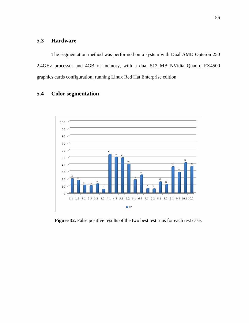
56
5.3 Hardware
The segmentation method was performed on a system with Dual AMD Opteron 250
2.4GHz processor and 4GB of memory, with a dual 512 MB NVidia Quadro FX4500
graphics cards configuration, running Linux Red Hat Enterprise edition.
5.4 Color segmentation
Figure 32. False positive results of the two best test runs for each test case.
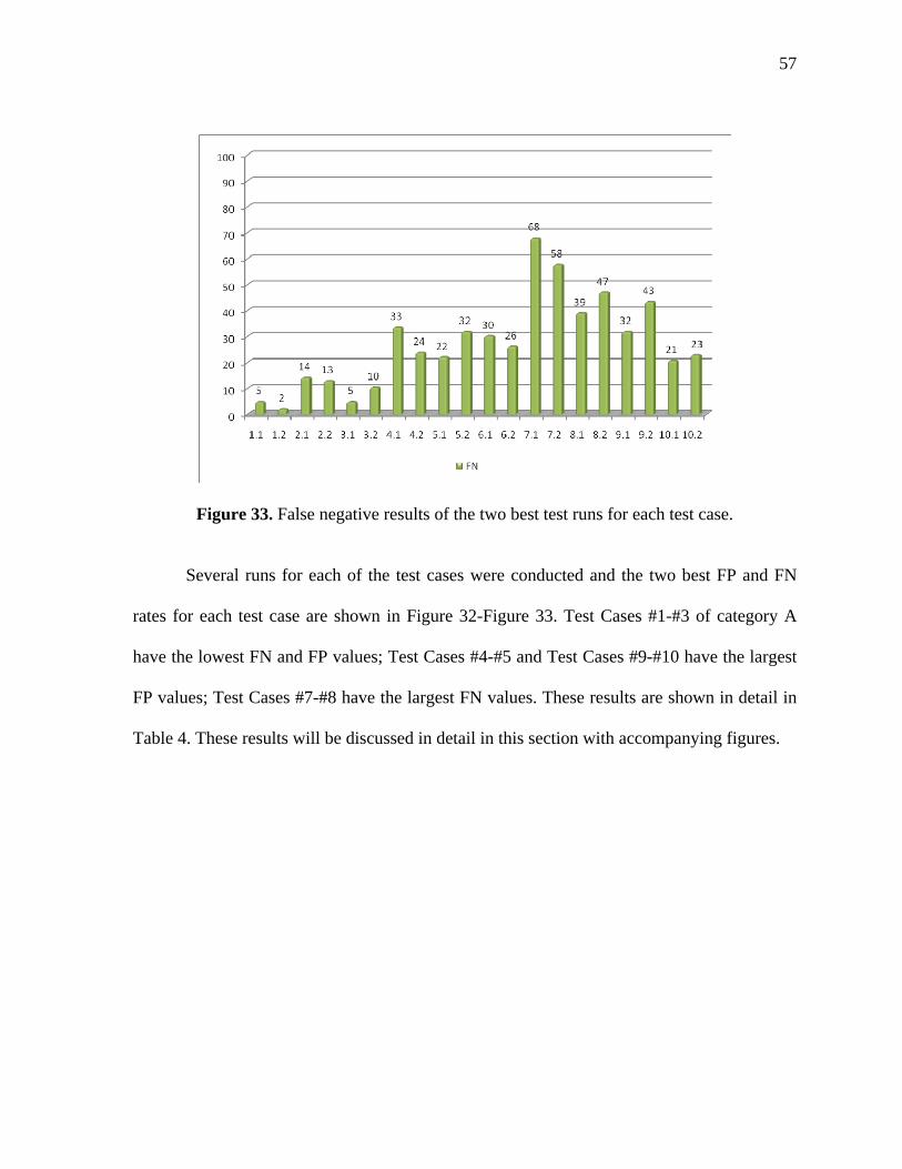
57
Figure 33. False negative results of the two best test runs for each test case.
Several runs for each of the test cases were conducted and the two best FP and FN
rates for each test case are shown in Figure 32-Figure 33. Test Cases #1-#3 of category A
have the lowest FN and FP values; Test Cases #4-#5 and Test Cases #9-#10 have the largest
FP values; Test Cases #7-#8 have the largest FN values. These results are shown in detail in
Table 4. These results will be discussed in detail in this section with accompanying figures.
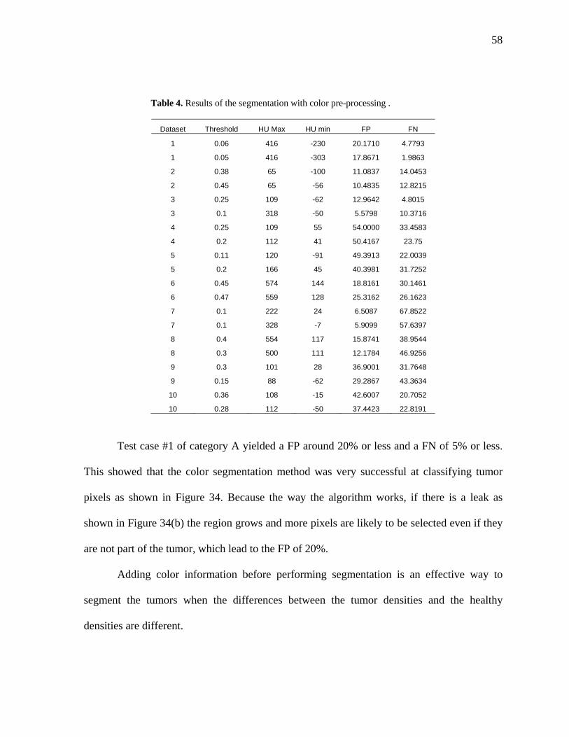
58
Table 4. Results of the segmentation with color pre-processing .
Dataset Threshold HU Max HU min FP FN
1 0.06 416 -230 20.1710 4.7793
1 0.05 416 -303 17.8671 1.9863
2 0.38 65 -100 11.0837 14.0453
2 0.45 65 -56 10.4835 12.8215
3 0.25 109 -62 12.9642 4.8015
3 0.1 318 -50 5.5798 10.3716
4 0.25 109 55 54.0000 33.4583
4 0.2 112 41 50.4167 23.75
5 0.11 120 -91 49.3913 22.0039
5 0.2 166 45 40.3981 31.7252
6 0.45 574 144 18.8161 30.1461
6 0.47 559 128 25.3162 26.1623
7 0.1 222 24 6.5087 67.8522
7 0.1 328 -7 5.9099 57.6397
8 0.4 554 117 15.8741 38.9544
8 0.3 500 111 12.1784 46.9256
9 0.3 101 28 36.9001 31.7648
9 0.15 88 -62 29.2867 43.3634
10 0.36 108 -15 42.6007 20.7052
10 0.28 112 -50 37.4423 22.8191
Test case #1 of category A yielded a FP around 20% or less and a FN of 5% or less.
This showed that the color segmentation method was very successful at classifying tumor
pixels as shown in Figure 34. Because the way the algorithm works, if there is a leak as
shown in Figure 34(b) the region grows and more pixels are likely to be selected even if they
are not part of the tumor, which lead to the FP of 20%.
Adding color information before performing segmentation is an effective way to
segment the tumors when the differences between the tumor densities and the healthy
densities are different.
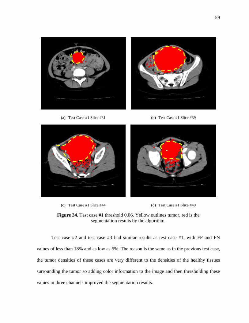
59
(a) Test Case #1 Slice #31 (b) Test Case #1 Slice #39
(c) Test Case #1 Slice #44 (d) Test Case #1 Slice #49
Figure 34. Test case #1 threshold 0.06. Yellow outlines tumor, red is the segmentation results by the algorithm.
Test case #2 and test case #3 had similar results as test case #1, with FP and FN
values of less than 18% and as low as 5%. The reason is the same as in the previous test case,
the tumor densities of these cases are very different to the densities of the healthy tissues
surrounding the tumor so adding color information to the image and then thresholding these
values in three channels improved the segmentation results.
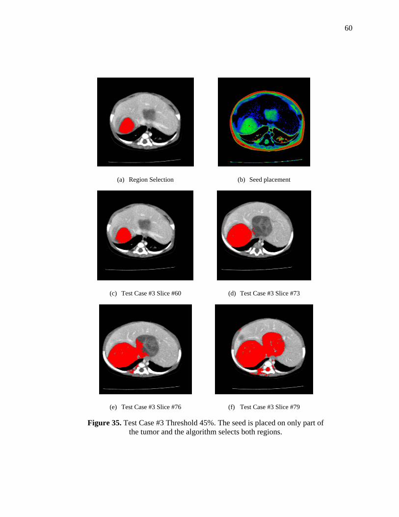
60
(a) Region Selection (b) Seed placement
(c) Test Case #3 Slice #60 (d) Test Case #3 Slice #73
(e) Test Case #3 Slice #76 (f) Test Case #3 Slice #79
Figure 35. Test Case #3 Threshold 45%. The seed is placed on only part of the tumor and the algorithm selects both regions.
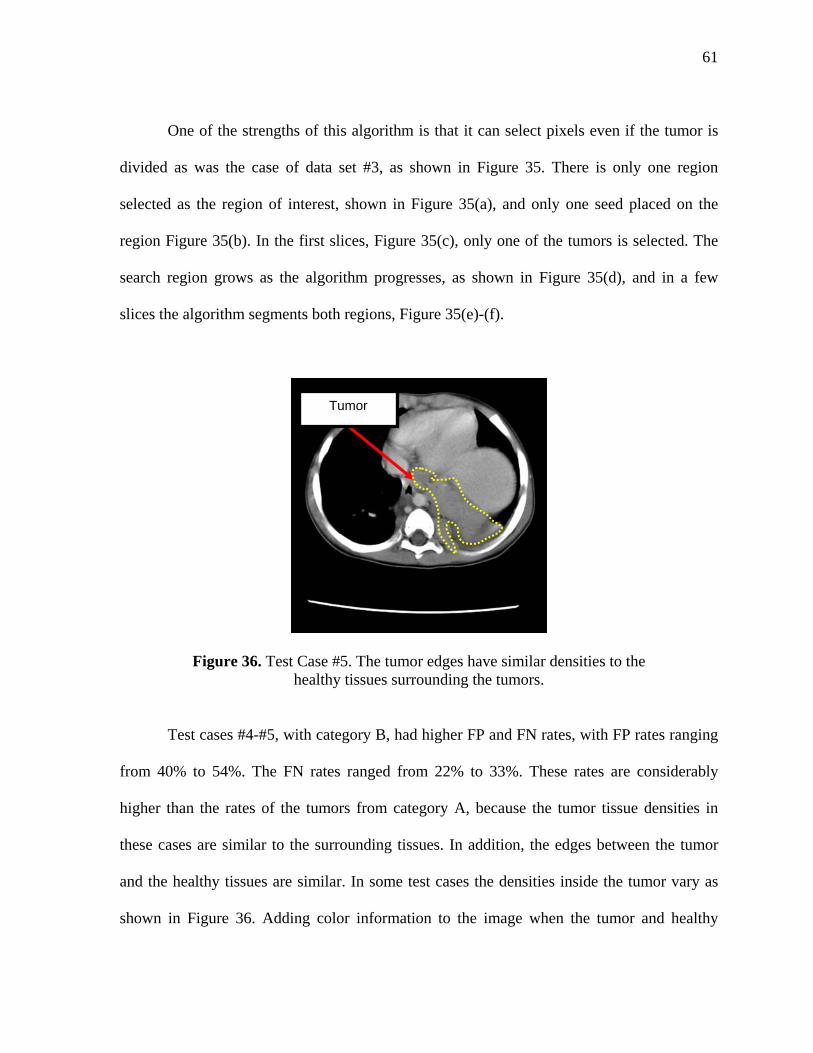
61
One of the strengths of this algorithm is that it can select pixels even if the tumor is
divided as was the case of data set #3, as shown in Figure 35. There is only one region
selected as the region of interest, shown in Figure 35(a), and only one seed placed on the
region Figure 35(b). In the first slices, Figure 35(c), only one of the tumors is selected. The
search region grows as the algorithm progresses, as shown in Figure 35(d), and in a few
slices the algorithm segments both regions, Figure 35(e)-(f).
Figure 36. Test Case #5. The tumor edges have similar densities to the healthy tissues surrounding the tumors.
Test cases #4-#5, with category B, had higher FP and FN rates, with FP rates ranging
from 40% to 54%. The FN rates ranged from 22% to 33%. These rates are considerably
higher than the rates of the tumors from category A, because the tumor tissue densities in
these cases are similar to the surrounding tissues. In addition, the edges between the tumor
and the healthy tissues are similar. In some test cases the densities inside the tumor vary as
shown in Figure 36. Adding color information to the image when the tumor and healthy
Tumor
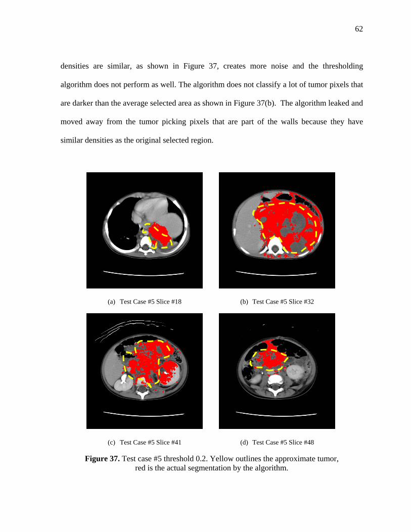
62
densities are similar, as shown in Figure 37, creates more noise and the thresholding
algorithm does not perform as well. The algorithm does not classify a lot of tumor pixels that
are darker than the average selected area as shown in Figure 37(b). The algorithm leaked and
moved away from the tumor picking pixels that are part of the walls because they have
similar densities as the original selected region.
(a) Test Case #5 Slice #18 (b) Test Case #5 Slice #32
(c) Test Case #5 Slice #41 (d) Test Case #5 Slice #48
Figure 37. Test case #5 threshold 0.2. Yellow outlines the approximate tumor, red is the actual segmentation by the algorithm.
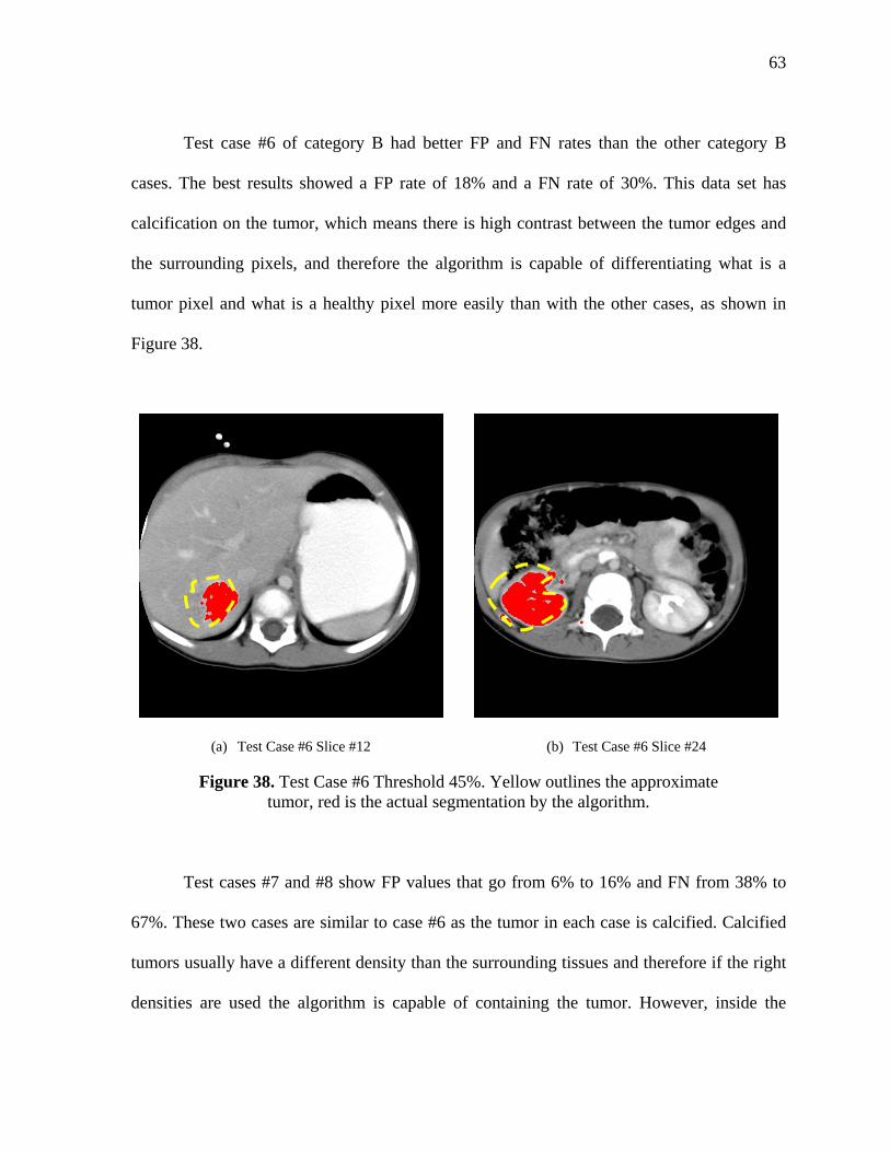
63
Test case #6 of category B had better FP and FN rates than the other category B
cases. The best results showed a FP rate of 18% and a FN rate of 30%. This data set has
calcification on the tumor, which means there is high contrast between the tumor edges and
the surrounding pixels, and therefore the algorithm is capable of differentiating what is a
tumor pixel and what is a healthy pixel more easily than with the other cases, as shown in
Figure 38.
(a) Test Case #6 Slice #12 (b) Test Case #6 Slice #24
Figure 38. Test Case #6 Threshold 45%. Yellow outlines the approximate tumor, red is the actual segmentation by the algorithm.
Test cases #7 and #8 show FP values that go from 6% to 16% and FN from 38% to
67%. These two cases are similar to case #6 as the tumor in each case is calcified. Calcified
tumors usually have a different density than the surrounding tissues and therefore if the right
densities are used the algorithm is capable of containing the tumor. However, inside the
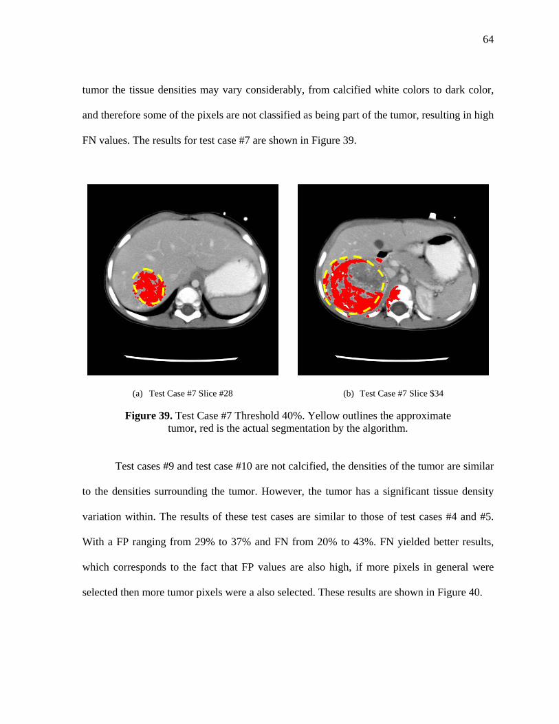
64
tumor the tissue densities may vary considerably, from calcified white colors to dark color,
and therefore some of the pixels are not classified as being part of the tumor, resulting in high
FN values. The results for test case #7 are shown in Figure 39.
(a) Test Case #7 Slice #28 (b) Test Case #7 Slice $34
Figure 39. Test Case #7 Threshold 40%. Yellow outlines the approximate tumor, red is the actual segmentation by the algorithm.
Test cases #9 and test case #10 are not calcified, the densities of the tumor are similar
to the densities surrounding the tumor. However, the tumor has a significant tissue density
variation within. The results of these test cases are similar to those of test cases #4 and #5.
With a FP ranging from 29% to 37% and FN from 20% to 43%. FN yielded better results,
which corresponds to the fact that FP values are also high, if more pixels in general were
selected then more tumor pixels were a also selected. These results are shown in Figure 40.
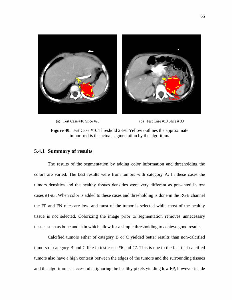
65
(a) Test Case #10 Slice #26 (b) Test Case #10 Slice # 33
Figure 40. Test Case #10 Threshold 28%. Yellow outlines the approximate tumor, red is the actual segmentation by the algorithm.
5.4.1 Summary of results
The results of the segmentation by adding color information and thresholding the
colors are varied. The best results were from tumors with category A. In these cases the
tumors densities and the healthy tissues densities were very different as presented in test
cases #1-#3. When color is added to these cases and thresholding is done in the RGB channel
the FP and FN rates are low, and most of the tumor is selected while most of the healthy
tissue is not selected. Colorizing the image prior to segmentation removes unnecessary
tissues such as bone and skin which allow for a simple thresholding to achieve good results.
Calcified tumors either of category B or C yielded better results than non-calcified
tumors of category B and C like in test cases #6 and #7. This is due to the fact that calcified
tumors also have a high contrast between the edges of the tumors and the surrounding tissues
and the algorithm is successful at ignoring the healthy pixels yielding low FP, however inside
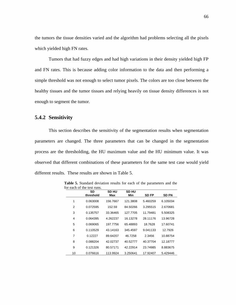
66
the tumors the tissue densities varied and the algorithm had problems selecting all the pixels
which yielded high FN rates.
Tumors that had fuzzy edges and had high variations in their density yielded high FP
and FN rates. This is because adding color information to the data and then performing a
simple threshold was not enough to select tumor pixels. The colors are too close between the
healthy tissues and the tumor tissues and relying heavily on tissue density differences is not
enough to segment the tumor.
5.4.2 Sensitivity
This section describes the sensitivity of the segmentation results when segmentation
parameters are changed. The three parameters that can be changed in the segmentation
process are the thresholding, the HU maximum value and the HU minimum value. It was
observed that different combinations of these parameters for the same test case would yield
different results. These results are shown in Table 5.
Table 5. Standard deviation results for each of the parameters and the for each of the test runs.
SD threshold
SD HU Max
SD HU Min SD FP SD FN
1 0.063008 156.7667 121.3808 5.460259 6.105034
2 0.072595 152.59 84.50266 3.295515 2.670681
3 0.135757 33.36465 127.7705 11.79481 5.508325
4 0.064395 4.262237 16.13278 28.11176 13.96728
5 0.069065 197.7756 65.48893 18.7628 17.60741
6 0.110529 43.14163 345.4597 9.041133 12.7926
7 0.12227 89.64207 46.7258 2.3456 10.88754
8 0.088204 42.02737 40.52777 40.37704 12.18777
9 0.121326 80.57171 42.22914 23.74985 8.883675
10 0.076616 113.9924 3.250641 17.92407 5.429446
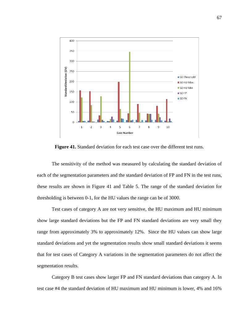
67
Figure 41. Standard deviation for each test case over the different test runs.
The sensitivity of the method was measured by calculating the standard deviation of
each of the segmentation parameters and the standard deviation of FP and FN in the test runs,
these results are shown in Figure 41 and Table 5. The range of the standard deviation for
thresholding is between 0-1, for the HU values the range can be of 3000.
Test cases of category A are not very sensitive, the HU maximum and HU minimum
show large standard deviations but the FP and FN standard deviations are very small they
range from approximately 3% to approximately 12%. Since the HU values can show large
standard deviations and yet the segmentation results show small standard deviations it seems
that for test cases of Category A variations in the segmentation parameters do not affect the
segmentation results.
Category B test cases show larger FP and FN standard deviations than category A. In
test case #4 the standard deviation of HU maximum and HU minimum is lower, 4% and 16%
68
respectively than the standard deviations for FP and FN which are 28% and 14%
respectively. Category B test cases are more sensitive to changes in the parameters than
Category A. Category C test cases show the most erratic deviations, some test cases such as
test case #7 show a FP and FN deviation of 2% and 11% than test case #8 which shows the
highest standard deviation for FP of 40%. Changes in the segmentation parameters for test
cases of Category B and Category C affect heavily the segmentation results because
Category B and Category C tumor cases have a higher variation in tissue density within the
tumor and densities between the tumor tissue and the surrounding tissues are closer, therefore
these cases are very dependent on the HU values, and even small variations of HU values
changes which tissues are selected and the segmentation results.
5.5 Grayscale segmentation
In this section the results of the grayscale segmentation algorithm are discussed.
Several runs of test cases #1, #5, #6, and #7 were done using a grayscale thresholding
segmentation algorithm. The test cases ranged from category A to category C.
To assess the effects of color pre-processing prior to segmentation, selected test cases
were segmented w the original HU values using the thresholding method discussed in
Chapter 3.3.
5.5.1 Algorithm
The initial region selected by the user determines the average HU value. This average
was then compared to each pixel in the image and multiplied by the distance over the search
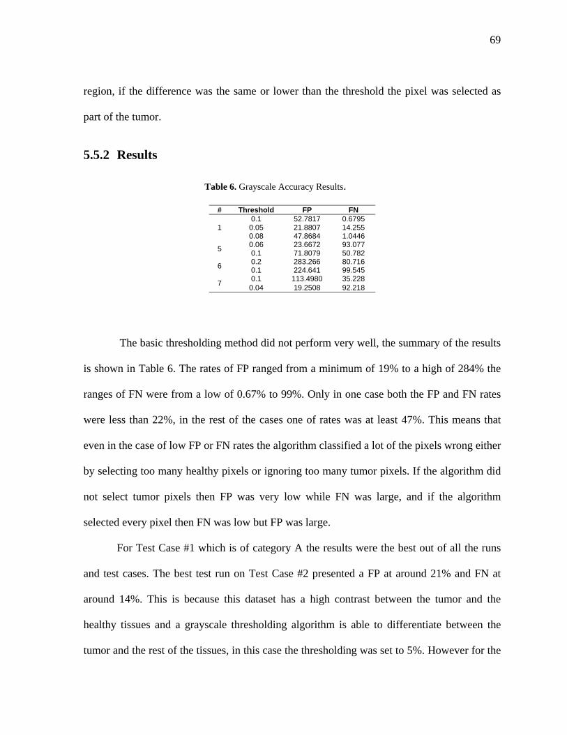
69
region, if the difference was the same or lower than the threshold the pixel was selected as
part of the tumor.
5.5.2 Results
Table 6. Grayscale Accuracy Results.
# Threshold FP FN
1 0.1 52.7817 0.6795
0.05 21.8807 14.255 0.08 47.8684 1.0446
5 0.06 23.6672 93.077 0.1 71.8079 50.782
6 0.2 283.266 80.716 0.1 224.641 99.545
7 0.1 113.4980 35.228
0.04 19.2508 92.218
The basic thresholding method did not perform very well, the summary of the results
is shown in Table 6. The rates of FP ranged from a minimum of 19% to a high of 284% the
ranges of FN were from a low of 0.67% to 99%. Only in one case both the FP and FN rates
were less than 22%, in the rest of the cases one of rates was at least 47%. This means that
even in the case of low FP or FN rates the algorithm classified a lot of the pixels wrong either
by selecting too many healthy pixels or ignoring too many tumor pixels. If the algorithm did
not select tumor pixels then FP was very low while FN was large, and if the algorithm
selected every pixel then FN was low but FP was large.
For Test Case #1 which is of category A the results were the best out of all the runs
and test cases. The best test run on Test Case #2 presented a FP at around 21% and FN at
around 14%. This is because this dataset has a high contrast between the tumor and the
healthy tissues and a grayscale thresholding algorithm is able to differentiate between the
tumor and the rest of the tissues, in this case the thresholding was set to 5%. However for the
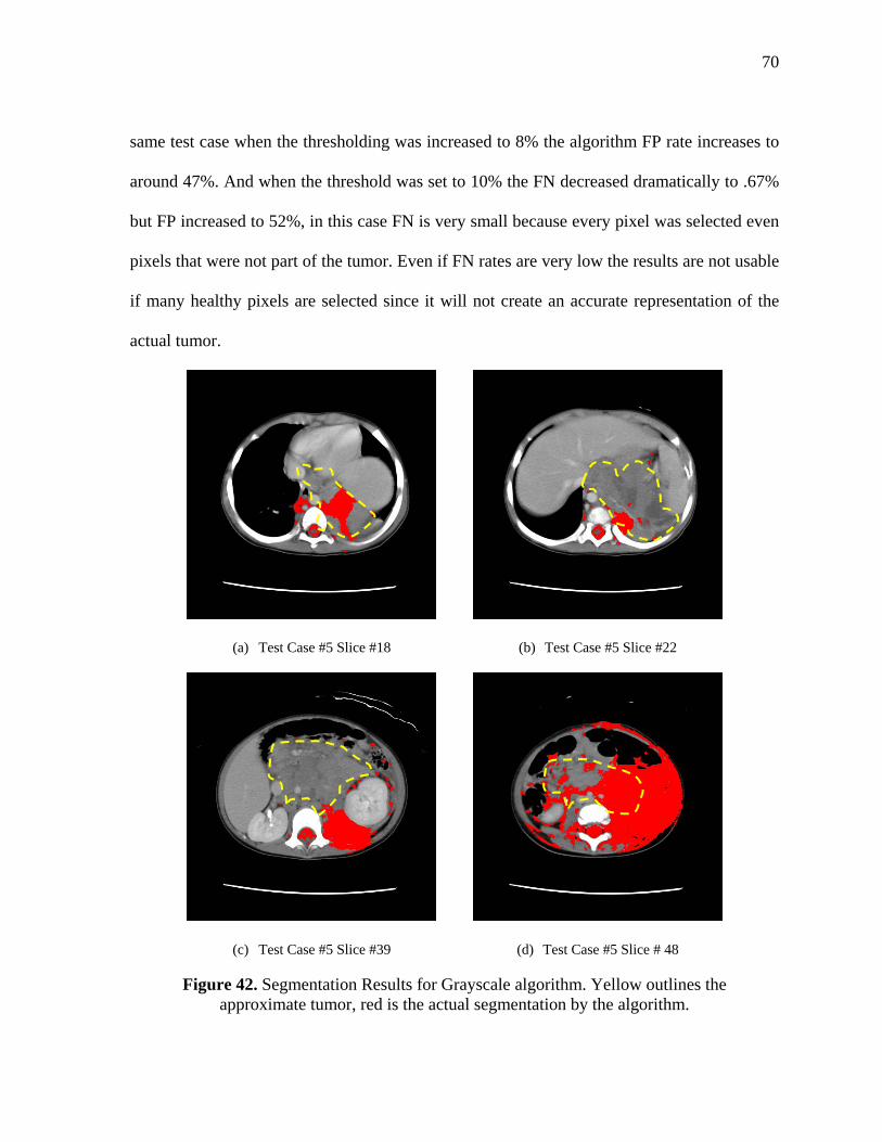
70
same test case when the thresholding was increased to 8% the algorithm FP rate increases to
around 47%. And when the threshold was set to 10% the FN decreased dramatically to .67%
but FP increased to 52%, in this case FN is very small because every pixel was selected even
pixels that were not part of the tumor. Even if FN rates are very low the results are not usable
if many healthy pixels are selected since it will not create an accurate representation of the
actual tumor.
(a) Test Case #5 Slice #18 (b) Test Case #5 Slice #22
(c) Test Case #5 Slice #39 (d) Test Case #5 Slice # 48
Figure 42. Segmentation Results for Grayscale algorithm. Yellow outlines the approximate tumor, red is the actual segmentation by the algorithm.
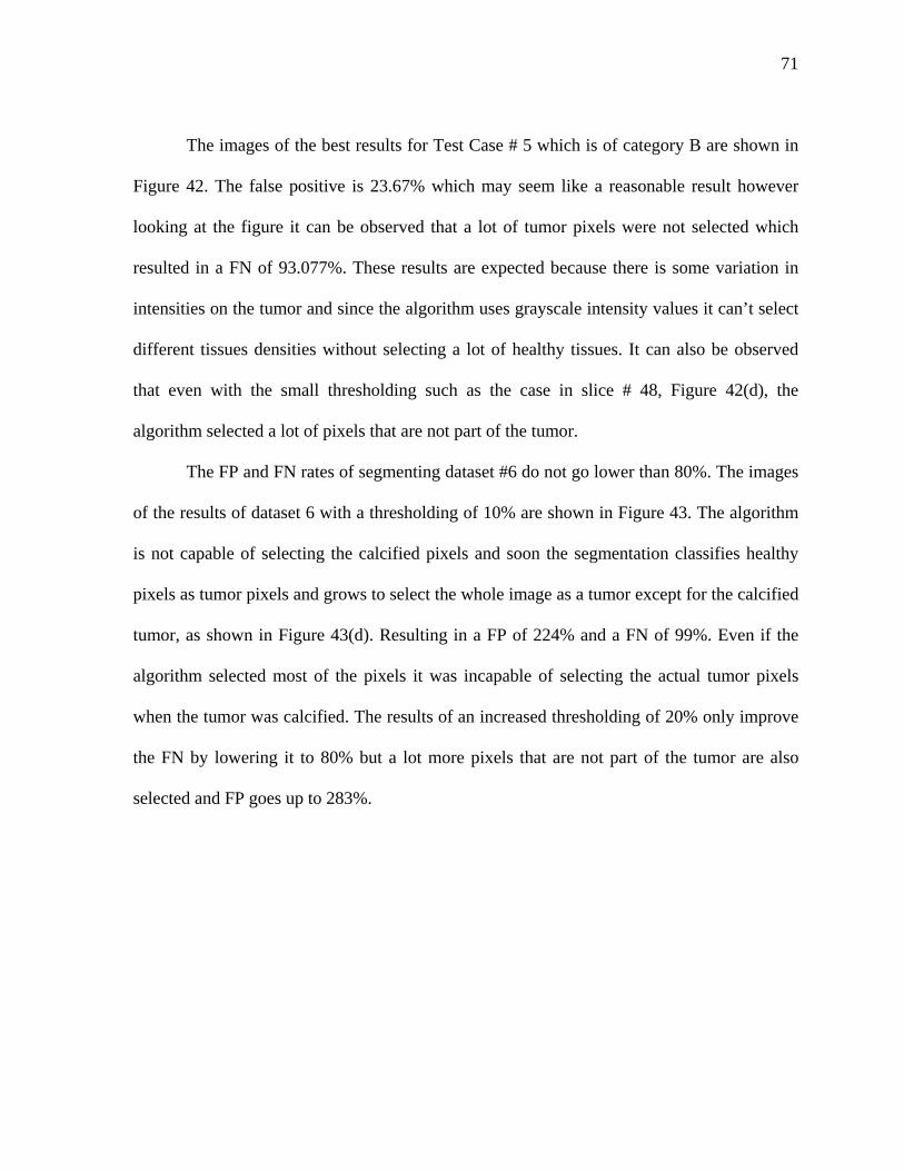
71
The images of the best results for Test Case # 5 which is of category B are shown in
Figure 42. The false positive is 23.67% which may seem like a reasonable result however
looking at the figure it can be observed that a lot of tumor pixels were not selected which
resulted in a FN of 93.077%. These results are expected because there is some variation in
intensities on the tumor and since the algorithm uses grayscale intensity values it can’t select
different tissues densities without selecting a lot of healthy tissues. It can also be observed
that even with the small thresholding such as the case in slice # 48, Figure 42(d), the
algorithm selected a lot of pixels that are not part of the tumor.
The FP and FN rates of segmenting dataset #6 do not go lower than 80%. The images
of the results of dataset 6 with a thresholding of 10% are shown in Figure 43. The algorithm
is not capable of selecting the calcified pixels and soon the segmentation classifies healthy
pixels as tumor pixels and grows to select the whole image as a tumor except for the calcified
tumor, as shown in Figure 43(d). Resulting in a FP of 224% and a FN of 99%. Even if the
algorithm selected most of the pixels it was incapable of selecting the actual tumor pixels
when the tumor was calcified. The results of an increased thresholding of 20% only improve
the FN by lowering it to 80% but a lot more pixels that are not part of the tumor are also
selected and FP goes up to 283%.
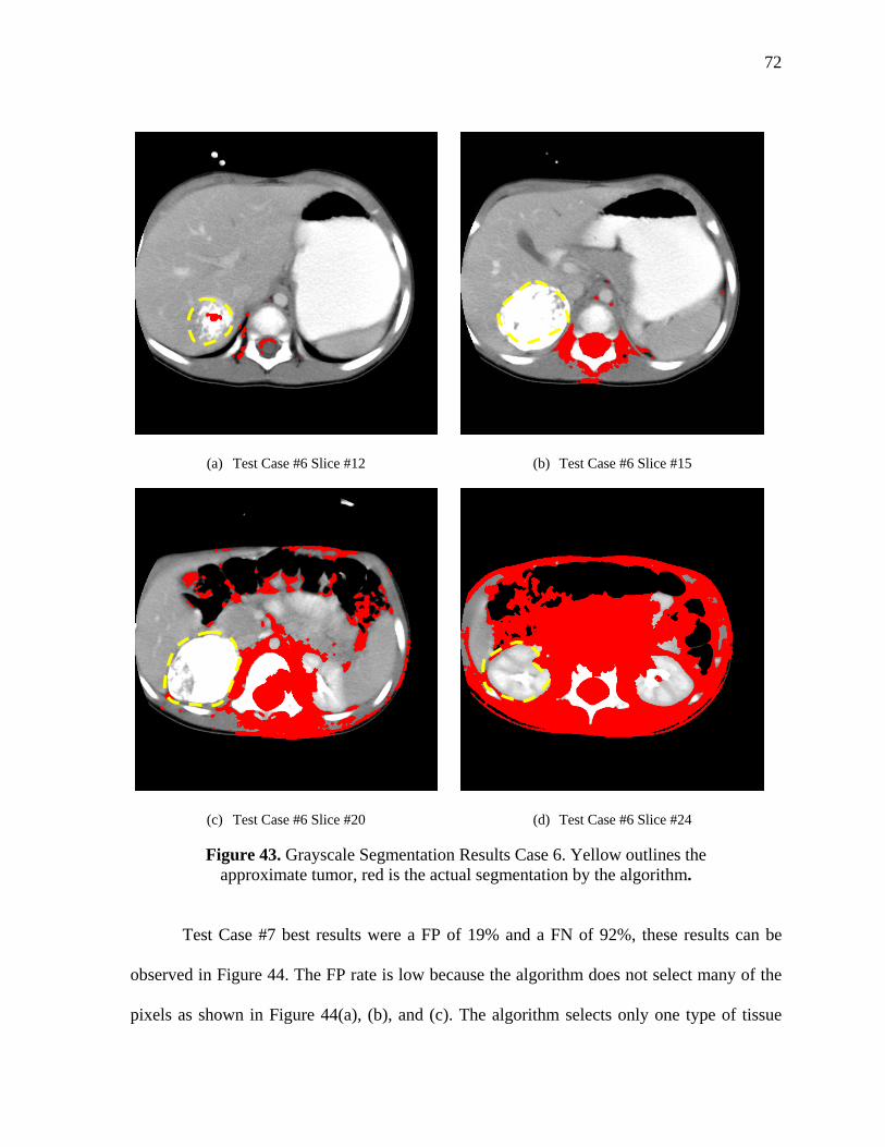
72
(a) Test Case #6 Slice #12 (b) Test Case #6 Slice #15
(c) Test Case #6 Slice #20 (d) Test Case #6 Slice #24
Figure 43. Grayscale Segmentation Results Case 6. Yellow outlines the approximate tumor, red is the actual segmentation by the algorithm.
Test Case #7 best results were a FP of 19% and a FN of 92%, these results can be
observed in Figure 44. The FP rate is low because the algorithm does not select many of the
pixels as shown in Figure 44(a), (b), and (c). The algorithm selects only one type of tissue
73
density and ignores the calcified tumor, or the pieces of tumor with different densities. As
shown in Figure 44(c) the segmentation starts to grow and by the last slice Figure 44(d) the
whole image is selected, except for the white pixels that in this case represent the actual
tumor. The thresholding technique creates a region leak outside the tumor of densities similar
in color with the region selected on the first slice but that unfortunately are not part of the
actual calcified tumor.
(a) Test Case #7 Slice #26 (b) Test Case #7 Slice #33
(c) Test Case #7 Slice #42 (d) Test Case #7 Slice #48
Figure 44. Test case #7. Yellow outlines the approximate tumor, red is the actual segmentation by the algorithm.
74
5.5.3 Limitations of Grayscale Thresholding
As the literature review of chapter 2 described and this section confirmed, basic
thresholding does not yield acceptable segmentation results. If the tumor is density is very
different than the healthy tissue density then this method produces adequate results as shown
in test case #1, however if the tumor densities are similar to healthy tissues densities as in the
case of test case #5, or if the tumor densities are varied as in test case #6 and test case #7
basic thresholding is not capable of producing results less than 90% in either FP or FN rates.
In the following section the grayscale and color methods will be compared and it will be
shown how adding color to the DICOM file and using the same thresholding technique but
with information in the RGB channels yields much better results, even with category C
tumors.
5.6 Comparison to other segmentation methods
While the results of the color segmentation are not as accurate as some other
elaborate segmentation algorithms the segmentation algorithm implemented here was a basic
thresholding technique that is not usually used for complex cases, comparing the
segmentation of basic thresholding between the color and grayscale cases the color
algorithms yielded much better results, as shown in Table 7 and Figure 45Figure 46. In each
of the test cases the color algorithm yielded better results, especially in difficult cases. Test
case #1 that corresponds to category A yielded the closest results between the two algorithms
which is expected since in this case the tumor densities are very different to healthy densities
and therefore simple thresholding can segment the tumor.
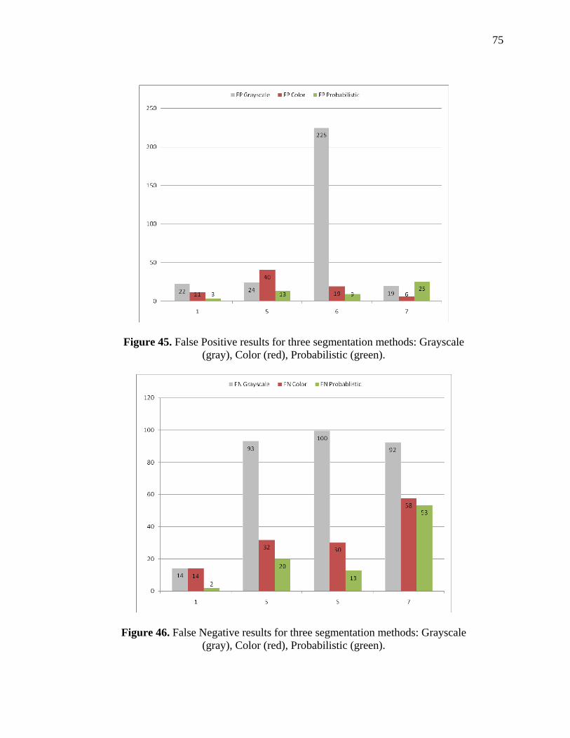
75
Figure 45. False Positive results for three segmentation methods: Grayscale (gray), Color (red), Probabilistic (green).
Figure 46. False Negative results for three segmentation methods: Grayscale (gray), Color (red), Probabilistic (green).
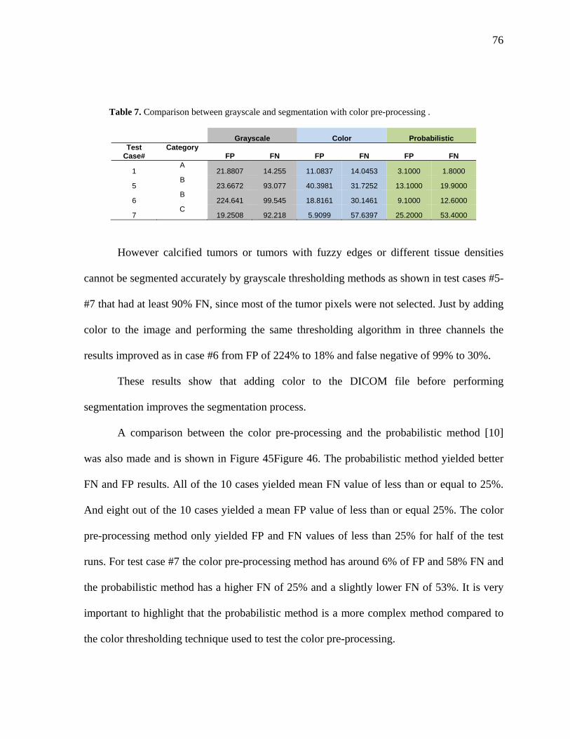
76
Table 7. Comparison between grayscale and segmentation with color pre-processing .
Grayscale Color Probabilistic Test
Case# Category
FP FN FP FN FP FN
1 A
21.8807 14.255 11.0837 14.0453 3.1000 1.8000
5 B
23.6672 93.077 40.3981 31.7252 13.1000 19.9000
6 B
224.641 99.545 18.8161 30.1461 9.1000 12.6000
7 C
19.2508 92.218 5.9099 57.6397 25.2000 53.4000
However calcified tumors or tumors with fuzzy edges or different tissue densities
cannot be segmented accurately by grayscale thresholding methods as shown in test cases #5-
#7 that had at least 90% FN, since most of the tumor pixels were not selected. Just by adding
color to the image and performing the same thresholding algorithm in three channels the
results improved as in case #6 from FP of 224% to 18% and false negative of 99% to 30%.
These results show that adding color to the DICOM file before performing
segmentation improves the segmentation process.
A comparison between the color pre-processing and the probabilistic method [10]
was also made and is shown in Figure 45Figure 46. The probabilistic method yielded better
FN and FP results. All of the 10 cases yielded mean FN value of less than or equal to 25%.
And eight out of the 10 cases yielded a mean FP value of less than or equal 25%. The color
pre-processing method only yielded FP and FN values of less than 25% for half of the test
runs. For test case #7 the color pre-processing method has around 6% of FP and 58% FN and
the probabilistic method has a higher FN of 25% and a slightly lower FN of 53%. It is very
important to highlight that the probabilistic method is a more complex method compared to
the color thresholding technique used to test the color pre-processing.
77
As expected, the grayscale case produced the worst results, the probabilistic method
yielded the best results and the color pre-processing method was in the middle. Even though
the color pre-processing method did not yield the best results the results improved
substantially the accuracy of the thresholding segmentation method. If the same approach is
used for the probabilistic method, if color is added as a pre-processing step it could improve
the accuracy of the current probabilistic method.
5.7 Timing
The method developed takes advantage of OpenGL textures to allow for the
visualization of the segmentation results of the current slice in real time. For the twenty cases
segmented the total time for the complete segmentation of the whole set was measured and
then it was divided by the number of slices, the results are shown in Table 8. If segmentation
is performed in the whole set of slices it takes a few seconds up to one minute if 251 slices
are being segmented such as test case #6. Tweaking values on one slice is performed in real
time, if the preferences selected to that slice want to be applied to the whole set then it takes
an average of 1/10 of a second per slice to show the results.
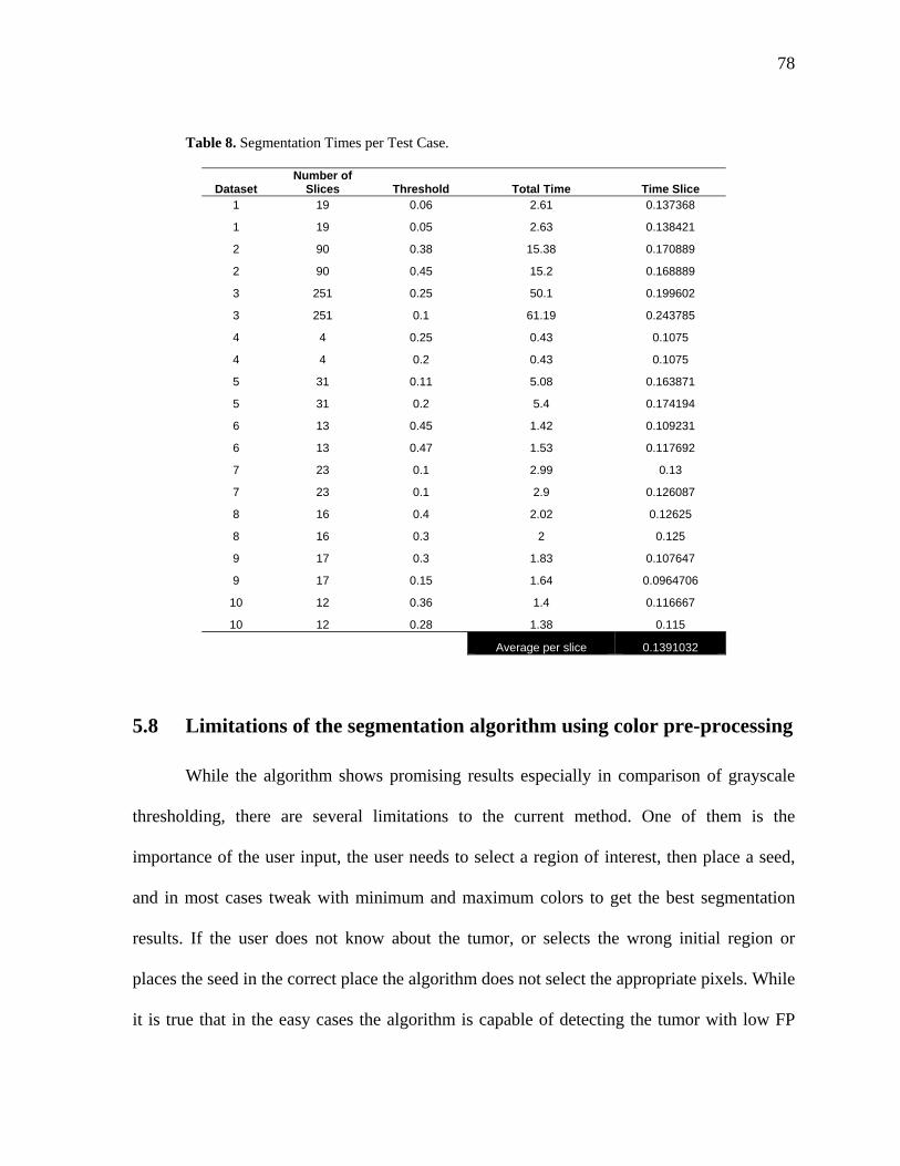
78
Table 8. Segmentation Times per Test Case.
Dataset Number of
Slices Threshold Total Time Time Slice 1 19 0.06 2.61 0.137368
1 19 0.05 2.63 0.138421
2 90 0.38 15.38 0.170889
2 90 0.45 15.2 0.168889
3 251 0.25 50.1 0.199602
3 251 0.1 61.19 0.243785
4 4 0.25 0.43 0.1075
4 4 0.2 0.43 0.1075
5 31 0.11 5.08 0.163871
5 31 0.2 5.4 0.174194
6 13 0.45 1.42 0.109231
6 13 0.47 1.53 0.117692
7 23 0.1 2.99 0.13
7 23 0.1 2.9 0.126087
8 16 0.4 2.02 0.12625
8 16 0.3 2 0.125
9 17 0.3 1.83 0.107647
9 17 0.15 1.64 0.0964706
10 12 0.36 1.4 0.116667
10 12 0.28 1.38 0.115
Average per slice 0.1391032
5.8 Limitations of the segmentation algorithm using color pre-processing
While the algorithm shows promising results especially in comparison of grayscale
thresholding, there are several limitations to the current method. One of them is the
importance of the user input, the user needs to select a region of interest, then place a seed,
and in most cases tweak with minimum and maximum colors to get the best segmentation
results. If the user does not know about the tumor, or selects the wrong initial region or
places the seed in the correct place the algorithm does not select the appropriate pixels. While
it is true that in the easy cases the algorithm is capable of detecting the tumor with low FP
79
and FN rates without the need of tweaking with the minimum and maximum colors, the user
still has to select a region of interest and place a seed.
Since this method is thresholding on three different channels the method is very
sensitive to tissue densities. In some cases if the color values are varied even by a little bit the
results vary a lot. For example test case #4, using the same threshold of 25% if the color
minimum is moved from 109 to 112, 3 values and the color maximum is decreases from 55
to 41, 14 values, the FP changes from 54% to 76% and FN changes from 33% to 11%.
Because the algorithm is only dependant on the position and on the densities if the wrong
maximum color and minimum color are chosen then the resulting FN and FP ranges will be
very high.
Due to the fact of the high sensitivity of the tissue densities the method also performs
poorly when the densities within a tumor are varied, selecting only a few pixels of the tumor
such as in test case #6 and #7, however it does not select a lot of pixels outside the tumor. In
a similar fashion when the edges of the tumor are fuzzy such as in cases #9-#10 the algorithm
picks a lot of pixels that are not part of the tumor.
80
6. CONCLUSIONS
6.1 Summary of conclusions
A framework to improve the accuracy of tumor segmentation from medical image
data was presented. This framework includes an interface for visualization of DICOM data in
2D and 3D. The framework introduced the idea of colorizing medical image by selecting a
region of interest, usually the tumor and colorizing the rest of the image with RGB values in
a linear fashion. This method also takes advantage of OpenGL textures to allow interactive
segmentation by having user tweak with the parameters in real time and visualize the results.
In the past colorization techniques have been implemented to achieve better
visualization results, such as colorizing black and white movies, however colorization
methods in medical image data to improve segmentation is a novel concept. To prove the
concept that colorizing or adding R, G, and B channels, information to an image to improve
segmentation a basic thresholding technique was implemented in grayscale and in color. The
method was very similar; the only difference was that instead of calculating the difference
between the original HU values for the grayscale case, the difference was calculated in RGB,
in three channels. The new method performed a lot better than the grayscale method in all the
cases, but especially in difficult cases tumors with calcification or tumors with different
densities. While the grayscale method had FN values of 90%, the color case had FN values
up to 57%. 10 out of the 20 test cases gave false positives of 25% or less, and 10 out of the
20 test runs gave false negatives of 25% or less. This new method promises a lot of
possibilities, however future work has to be done on the proposed method.
81
It is important to note that at this point human input is fundamental to this method and
segmentation methods in general. The segmentation algorithms developed to this day are not
completely accurate and when the results are helping to determine surgical planning there is
no room for errors.
6.2 Future work
Future work on this framework can be divided into four ways: (a) adding different
and more complex segmentation algorithms using color information; (b) trying different
color pre-processing methods (c) using GPU and shaders to increase the speed of the results;
(d) different ways to move the seed point; (e) isolate the sources of error; (g) improve the
user interface.
Taking into account that adding color to the basic grayscale thresholding technique
improved results there is a possibility that adding more complex color segmentation
algorithms can yield even better results. Many successful algorithms that are used for tumor
segmentation are only focused on grayscale methods since medical data is obtained only in
reference to HU values. If adding color to the images improves the basic method other
methods can also be improved in this fashion. Probabilistic segmentation methods, fuzzy
logic, and region grow can be methods to be tested using color pre-processing techniques and
then segmentation. These new methods may decrease the need of user input.
A simple color pre-processing method that added RGB information from red to blue
in a linear fashion was implemented, however other methods can also be tested to see if they
improved segmentation results. Adding more colors instead of just RGB or even changing
82
color spaces for example using HSI instead of RGB may yield different results that could
make the framework more robust.
The method proposed in this work uses textures to visualize the results to be tweaked
in real time. Using shaders offers another possibility instead of generating textures every time
a parameter is changed, and perhaps shaders will improve the speed of the method. While the
method is already fast improving the speed allows for more complicated methods to be
implemented without sacrificing the speed of the framework.
The method only explores one way to move the seed point which is by placing the
seed on the center of the previous segmented slice. Other ways to move the seed point may
yield better results and should be explored in future work.
Several parameters are used to calculate the segmentation region and it is not clear
which parameters have the most influence on the results, a study needs to be developed to
isolate the sources of error in the method and segmentation in general.
The user interface right now has not been tested and has only been used by the
developers. Testing should be performed to improve the user experience and make the
application easier to use.
83
ACKNOWLEDGMENTS
I would first like to acknowledge my parents and my brother. Also my extended
family which includes my grandparents, uncles, cousins and my old friends: “the band”, the
“pecados”, and the fantastic four. You always believed in me and helped me to get into a
better university even if it meant being away from all of you, and you motivated me to take
advantage of the great opportunity.
I also want to thank Eliot Winer because he gave me the opportunity to do a masters.
He was patient with my lack of programming skills and at the same time pushed me enough
to try new things and learn more.
To Eric Foo because he was there day through day helping me with concepts, code,
and the revision of this thesis.
Ken Kopecky because when I asked if I should do A or B he said C, which was very
complicated at first but resulted in a big important part of my research. Also because when I
see his code I think pretty and it pushes me to improve my coding skills.
To the watch research group especially Vijay K, Brandon N, Catherine P, Andrew k
because they helped me with random stuff from makefile files to Socketing.
And to all my friends, especially Curt Putney, Grego Worhland, Jason Morgan, Len
Martinez, Al Cosme, and Nick Johnston because they have helped a lot in the last few
months with things like posters, to grammar and spelling.
84
REFERENCES
[1] Gonzalez, Rafael C., and Richard E. Woods. Digital Image Processing. New
York: Addison-Wesley, 2008.
[2] Bankman, Isaac. Handbook of Medical Imaging: Processing and Analysis.
California: Academic Press, 2000.
[3] Imaginis: Brief History of CT. 13 Sep. 2007. Imaginis. 22 Oct. 2008.
<http://www.imaginis.com/ct-scan/history.asp>
[4] Hornak, Joseph. The Basics of MRI. 22 Oct. 2008.
<http://www.cis.rit.edu/htbooks/mri/inside.htm>
[5] Nema. Digital Imaging and Communications in Medicine. 22 Oct. 2008
<http://medical.nema.org/>
[6] Pham, Dzung.L., Chenyang Y. Xu, and Jerry L. Prince. “A Survey of Current
Methods in Medical Image Segmentation.” Medical Image Analysis 2.1 (1998): 1-36.
[7] Ayres, F.J, et al. “Estimation of the Tissue Composition of the Tumor Mass in
Neuroblastoma Using Segmented CT Images.” Medical & Biological Engineering and
Computing 42.3 (2004): 266-77.
[8] Intuitive Surgical: da Vinci Surgical System. 22 Oct. 2009.
<http://www.intuitivesurgical.com/products/davinci_surgicalsystem/index.aspx>
[9] Marescaux, Jaques., et al. “Transcontinental Robot-Assisted Remote Telesurgery:
Feasibility and Potential Applications.” Annals of Surgery 245.4 (2002): 487-92.
85
[10] Foo, Eric. “A Framework for Segmentation and Interactive Immersive
Visualization of Medical Image Data.” Diss. Iowa State University, 2008.
[11] Pham, Dzung L., Chenyang Xu, and Jerry L. Prince. “Current Methods in
Medical Image Segmentation.” Annual Review of Biomedical Engineering 2 (2000): 315-
337.
[12] Clarke, L.P. et al. “MRI Segmentation: Methods and Applications.” Magnetic
Resonance Imaging 13.3 (1995): 343-68.
[13] Hadwiger, Marcus, et al. State of the Art Report 2004 on GPU Based
Segmentation. Vienna, Austria: VRVis Research Center, 2004.
[14] Fan, Jianping, et al. “Automatic Image Segmentation by Integrating Color-Edge
Extraction and Seeded Region Growing.” IEEE Transactions on Image Processing 10 (2001):
1454-66.
[15] Rajapakse, Jagath C., et al. “Statistical Approach Segmentation Single-Channel
Cerebral MR Images.” IEEE Transactions on Medical Imaging 16 (1997): 176-86.
[16] Sezgin, Methmet, and Bulent Sankur. “Survey Over Image Thresholding
Techniques and Quantitative Performance Evaluation.” Jounral of Electronic Imaging 13.1
(2004): 146-65.
[17] Freixenet, F., et al. “Yet Another Survey on Image Segmentation: Region and
Boundary Information Integration.” Lecture Notes In Computer Science: Proceedings of the
7th European Conference on Computer Vision-Part III, Denmark, 28-31 May 2002. Ed. A
Hayden. Berlin: Springer, 2002. 408-422.
[18] Hojjatoleslami, S.A., and J. Kittler. “Region Growing: A New Approach.” IEEE
Transactions on Image Processing 7 (1998): 1079-84.
86
[19] Pohle, Regina, and Klaus, Toennies. “Segmentation of Medical Images Using
Adaptive Region Growing.” SPIE Medical Imaging 4322 (2001): 1337-46.
[20] Berkhin, P. “Survey in Clustering Data Mining Techniques.” Grouping
Multidimensional Data: Recent Advances in Clustering. Ed. Jacob Kogan. Berlin: Springer,
2006. 25-71.
[21] Zhang, Dao-Qiang, and Song-Can Chen. “A Novel Kernelized Fuzzy C-means
Algorithm with Application in Medical Image Segmentation.” Artificial Intelligence in
Medicine 32.1 (2004): 37-50.
[22] Held, Karsten, et al. “Markov Random Field Segmentation of Brain MRI
Images.” IEEE Transactions on Medical Imaging 16 (1997): 878-886.
[23] Zhang, Yongye, et al. “Segmentation of Brain MR Images through a Hidden
Markov Random Field Model and the Expectation-maximization Algorithm.” IEEE
Transactions on Medical Imaging 20 (2001): 45-57.
[24] Vincken, Koen. “Probabilistic Multiscale Image Segmentation. “ IEEE
Transactions on Pattern Analysis and Machine Intelligence 19 (1997): 109-120.
[25] Xu, Chenyang, et al. “Image Segmentation Using Deformable Models.”
Handbook of Medical Imaging: Medical Image Processing and Analysis. Ed. Jacob Beutel.
Bellingham: SPIE Press, 2000. 129-74.
[26] Kaus, Michael R., et al. “Automated Segmentation of the Left Ventricle in
Cardiac MRI.” Medical Image Analysis 8.3 (2003): 245-54.
[27] McInerney, Tim, and Demetri Terzopoulos. “Deformable Models in Medical
Image Analysis: a Survey.” Medical Image Analysis 1.2 (1996): 91-108.
87
[28] Reddick, Wilburn E., et al. “Automated Segmentation and Classification of
Multispectral Magnetic Resonance Images of Brain Using Artificial Neural Networks.” IEE
Transactions on Medical Imaging 16 (1997): 911-18.
[29] Huang, Yu-Len, and Dar-Ren Chen. “Watershed Segmentation for Breast Tumor
in 2-D Sonography.” Ultrasound in Medicine & Biology 30.5 (2004): 625-32.
[30] Egmont-Patersen, M., D. de Ridder, and H. Handels. “Image Processing with
Neural Networks – a Review.” Pattern Recognition 35 (2002): 2279-301.
[31] Saha, Punam K, Jayaram K . Udupa, and Dewey Odhner. “Scale-Based Fuzzy
Connected Image Segmentation: Theory, Algorithms, and Validation.” Computer Vision and
Image Understanding 77 (2000): 145-174.
[32] Udupa, Jayram K., and Supun Samarasekera. “Fuzzy Connectedness and Object
Definition: Theory, Algorithms, and Applications in Image Segmentation.” Graphical
Models and Image Processing 58 (1996): 246-61.
[33] Moonis, Gul, et al. “Estimation of Tumor Volume with Fuzzy-Connectedness
Segmentation of MR Images.” American Journal of Neuroradiology 23 (2002): 356-63.
[34] Lorenzo-Valdés, M., et al. “Atlas-Based Segmentation and Tracking of 3D
Cardiac MR Images Using Non-rigid Registration.” Medical Image Computing and
Computer-Assisted Intervention-MICCAI 2002, 5th International Conference Proceedings,
Tokyo, 25-28 September 2002. Ed. Takeyoshi Dohi. Berlin: Springer. 642-50.
[35] Gibou, Frédéric, and Ronald Fedkiw. A Fast Hybrid k-Means Level Set
Algorithm for Segmentation. California: Standford University Computer Science
Department, 2002.
88
[36] Atkins, M. Stella, and Blair T. Mackiewich. “Fully Automatic Segmentation of
the Brain in MRI.” IEEE Transactions on Medical Imaging 17 (1998): 98-107.
[37] Cheng, H.D., et al. “Color Image Segmentation: Advances and Prospects.”
Pattern Recognition 34 (2001): 2259-81.
[38] Levin, Anat, Dani Lischinski, and Yair Weiss. “Colorization Using
Optimization.” Proceedings of the 2004 SIGGRAPH Conference. Ed. John C.Hart. New
York: ACM, 2004. 689-94.
[39] Welsh, Tomihisa, Michael Ashikhim, and Klaus Mueller. “Transferring Color to
Greyscale Images.” International Conference on Computer Graphics and Interactive
Techniques: Proceedings of the 29th Annual Conference on Computer Graphics and
Interactive Techniques, San Antonio, Texas, 23-26 July 2002. New York: ACM, 2002. 277-
80.
[40] Sapiro, Guillermo. “Inpainting the Colors.” IEEE International Conference on
Image Processing, 2005. 2005. 698-701.
[41] Pfister, Hanspeter, et al. “The Transfer Function Bake-off.” IEEE Computer
Graphics and Applications 21 (2001): 16-22.
[42] He, Taosong, et al. “Generation of Transfer Functions with Stochastic Search
Techniques.” IEEE Visualization: Proceedings of the 7th Conference on Visualization ’96,
San Francisco, California, 28-29 October 1996. Ed. Roni Yagel. CA: IEEE Computer
Society, 1996. 227-34.
[43] Yatziv, Liron, and Guillermo Sapiro. “Fast Image and Video Colorization Using
Chrominance Blending.” IEEE Transactions on Image Processing 15 (2006): 1120-29.
89
[44] Blasi, Di, and Reforgiatio Recupero. “Fast Colorization of Gray Images.”
Proceedings Eurographics Italian Chapter, 2003. 2003.
[45] Chen, Tongbo, et al. “Grayscale Image Matting and Colorization.” Proceedings
of Asian Conference on Computer Vision, Korea, 2004. 2004. 1165-69.
[46] Horiuchi, Takahiko, and Sayaka Hirano. “Colorization Algorithm for Grayscale
Image by Propagating Seed Pixels.” International Conference on Image Processing, 2003.
2003. 457-60.
[47] Tzeng, Fan-Yin, Eric B. Lum, and Kwan-Liu Ma. “A Novel Interface for
Higher-Dimensional Classification of Volume Data.” Proceedings of the 14th IEEE
Visualization, 22-24 October 2003. Washington, DC: IEEE Computer Society, 2003. 505-12.
[48] Silverstein, Jonathan C., Nigel M. Parsad, and Victor Tsirline. “Automatic
Perceptual Color Map Generation for Realistic Volume Visualization.” Journal of
Biomedical Informatics 41 (2008): 927-35.
[49]Pelizzari, Charles A., et al. “Volumetric Visualization of Anatomy for Treatment
Planning.” International Journal of Radiation Oncology, Biology and Physics 34.1 (1996):
205-11.
[50] Li, C.H., and P.C. Yuen. “Regularized Color Clustering in Medical Image
Database.” IEEE Transactions on Medical Imaging 19 (2000): 1150-55.
[51]Lucchese, L., and S.K. Mitra. “Color Image Segmentation: A State-of-the-Art
Survey.” Proceedings Indian National Science Academy, India. 2001. 207-21.
[52] Skarbek, Wladyslaw, and Andreas Koschan. “Colour Image Segmentation – A
Survey - .” Berlin: Institute for Technical Informatics, University of Berlin, 1994.
90
[53] Lin, Xueyin, and Shaoyun Chen. “Color Image Segmentation Using Modified
HSI System for Road Following.” IEEE International Conference on Robotics and
Automation, Proceedings, California, 9-11 April 1991. 1991. 1996-2003.
[54] Cheng, H.D., X.H. Jiang, and Jingli Wang. “Color Image Segmentation Based on
Homogram Thresholding and Region Merging.” Pattern Recognition 35 (2002): 373-93.
[55] Verikas, A., K. Malmqvist, and L. Bergman. “Colour Image Segmentation by
Modular Neural Network.” Pattern Recognition Letters 18 (1997): 173-85.
[56] Cremers, Daniel, Mikael Rousson, and Rachid Deriche. “A Review of Statistical
Approaches to Level Set Segmentation: Integrating Color, Texture, Motion and Shape.”
International Journal of Computer Vision. 72 (2006): 195-215.
[57] Volview. 8 Nov. 2008 <http://www.kitware.com/products/volview.html>
[58] OsiriX Imaging Software. 9 Nov. 2008 < http://www.osirix-viewer.com/>
[59] “Morphology Fundamentals: Dilation and Erosion.” The MathWorks. 9 Nov.
2008 <http://www.mathworks.com/access/helpdesk/help/toolbox/images/index.html?/
access/helpdesk/help/toolbox/images/f18-12508.html>
[60] DCMTK – DICOM Toolkit. 9 Nov. 2008 <http://dicom.offis.de/dcmtk>
[61] OpenGL. 9 Nov. 2008 <http://www.opengl.org/>
[62] The Visualization Toolkit (VTK). 9 Nov. 2008 <http://www.vtk.org/>
[63] Corona. 9 Nov. 2008 <http://corona.sourceforge.net/>
[64] VR Juggler. 9 Nov. 2008 <http://www.vrjuggler.org/>