an intro duction to r for dynamic mo dels in...

CONTENTS 1

An introduction to R for dynamic models in biologyLast compile: June 6, 2006

Stephen P. Ellner1 and John Guckenheimer2

1Department of Ecology and Evolutionary Biology, and2Department of Mathematics

Cornell University, Ithaca NY 14853

Contents

1 Interactive calculations 4

2 An interactive session: fitting a linear regression model 6

3 Script files and data files 7

4 Vectors 10

5 Matrices 14

5.1 cbind and rbind . . . . . . . . . . . . . . . . . . . . . . . . . . . . . . . . . . . . . . . . . . 14

6 Iteration (“Looping”) 17

6.1 For-loops . . . . . . . . . . . . . . . . . . . . . . . . . . . . . . . . . . . . . . . . . . . . . 17

6.2 While-loops . . . . . . . . . . . . . . . . . . . . . . . . . . . . . . . . . . . . . . . . . . . . 19

7 Branching 21

8 Numerical operations with Matrices 22

8.1 Eigenvalues and eigenvectors . . . . . . . . . . . . . . . . . . . . . . . . . . . . . . . . . . 23

8.2 Eigenvalue sensitivities and elasticities . . . . . . . . . . . . . . . . . . . . . . . . . . . . . 24

8.3 Finding the eigenvalue with largest real part . . . . . . . . . . . . . . . . . . . . . . . . . . 25

9 Creating new functions 26

10 A simulation project 27

11 Coin tossing and Markov Chains 28

11.1 Markov chains and residence times . . . . . . . . . . . . . . . . . . . . . . . . . . . . . . . 30

12 The Hodgkin-Huxley model 31

CONTENTS 2

12.1 Getting started . . . . . . . . . . . . . . . . . . . . . . . . . . . . . . . . . . . . . . . . . . 33

13 Solving systems of di!erential equations 35

13.1 Always use lsoda! . . . . . . . . . . . . . . . . . . . . . . . . . . . . . . . . . . . . . . . . . 38

13.2 The logs trick . . . . . . . . . . . . . . . . . . . . . . . . . . . . . . . . . . . . . . . . . . . 39

14 Equilibrium points and linearization 40

15 Phase-plane analysis and the Morris-Lecar model 42

16 Simulating Discrete-Event Models 44

17 Simulating dynamics in systems with spatial patterns 46

17.1 General method of lines . . . . . . . . . . . . . . . . . . . . . . . . . . . . . . . . . . . . . 48

18 References 49

Preface

These notes for computer labs accompany our textbook Dynamic Models in Biology (Princeton Univer-sity Press 2006), but they can also be used as a “standalone” introduction to R as a scripting language forsimulating dynamic models of biological systems. They are based in part on course materials by formerTAs Colleen Webb, Jonathan Rowell and Daniel Fink at Cornell University, Lou Gross (University ofTennessee) and Paul Fackler (NC State University), and on the book Getting Started with Matlab byRudra Pratap (Oxford University Press). We also have drawn on the documentation supplied with R(R Core Development Team 2005).

The current home for these notes is www.cam.cornell.edu/!dmb/DMBsupplements.html, a web pagefor the textbook that we maintain ourselves. If that fails, an up-to-date link should be in the book’slisting at the publisher (www.pupress.princeton.edu). Parallel notes and script files for Matlab arealso available at those sites.

Sections 1-7 are a general introduction to some basics of R programming. We generally cover those in 2or 3 2-hour lab sessions, depending on how much previous experience students have had. Rather thanlecturing on these sections, we have students work through them individually, asking for help as neededand having us or a TA check their exercise solutions. These sections contain many sample calculations.It is important to do them yourselves – type them in at your keyboard and see what happens on yourscreen – to get the feel of working in R . Exercises in the middle of a section should be done immediatelywhen you get to them, and make sure that you have them right before moving on. Exercises at the endsof sections may be more challenging and more appropriate as homework exercises. However the exercisesare all straightforward applications of the programming techniques being taught.

The subsequent sections are linked to our textbook in fairly obvious ways. For example, section 8 onmatrix computations goes with Chapter 2 on matrix models for structured populations, and section 15on phase-plane analysis of the Morris-Lecar model accompanies the corresponding section in Chapter 5.Some exercises in these sections are designed as ’warmups’ for exercises in the textbook, such as simpleexamples of agent-based (discrete-event) models as a warmup for agent-based simulation of infectious

CONTENTS 3

disease dynamics.

What is R ?

R is an object-oriented scripting language that combines

• the programming language S developed by John Chambers (Chambers and Hastie 1988, Chambers1998).

• a user interface with a few basic menus and extensive help facilities.

• an enormous set of functions for classical and modern statistical data analysis and modeling.

• graphics functions for visualizing data and model output.

R is an open-source project (R Core Development Team 2005) available free via the Web (see below).Originally a research project in statistical computing (Ihaka and Gentlemen 1996) it is now managed bya team that includes a number of well-regarded statisticians, and is widely used by statistical researchersand a growing number of theoretical biologists. The commercial implementation of the S language (calledS-plus) o!ers a “point and click” interface that R lacks. However for our purposes this is outweighed by thefact that S-plus still lacks some essential tools for simulating dynamic models. The standard installationof R includes extensive documentation, including an introductory manual and a comprehensive referencemanual. At this writing, R mostly follows version 3 of the S language, but some packages are startingto use version 4 features. These notes refer only to version 3 of S. We also limit ourselves to graphicsfunctions in the base graphics package (you’ll have to learn lattice graphics on your own).

The main sources for R are CRAN (cran.r-project.org) and its mirrors. You can get the source code,but most users will prefer a precompiled version. To get one from CRAN, click on the link for your OS,continue to the folder corresponding to your OS version, and find the appropriate download file for yourcomputer.

For Windows or OS X, R is installed by launching the downloaded file and following the on-screeninstructions. At the end you’ll have an R icon on your desktop that can be used to launch the program.Installing versions for LINUX or UNIX is more complicated and idiosyncratic (which will not bother thecorresponding users), but many recent LINUX distributions include a fairly up-to-date version of R .

For Windows PCs we strongly suggest that you edit the file Rconsole in R ’s etc folder and change theline MDI=yes to MDI=no, and also edit Rprofile to un-comment the line options(chmhelp=TRUE) byremoving the # at the start of the line. These changes allow R ’s command and graphics windows tomove independently on the desktop, and selects the most powerful version of the help system.

This document was written at a Windows PC and may sometimes refer to Windows-specific aspects ofR . We will be happy to make changes as these lapses are brought to our attention.

Statistics in R

Some of the important functions and libraries (collections of functions) for data analysis and statisticalmodeling are summarized in Table 1. The book Modern Applied Statistics with S by Venables and Ripleygives a good practical overview, and a list of available libraries and their contents is available at CRAN(www.cran.r-project.org, click on Package sources). Maindonald (2004) and Verzani (2002) – bothavailable online – present the basics of statistical data analysis and graphics in R . For the most part,we are not concerned here with this side of R .

1 INTERACTIVE CALCULATIONS 4

aov, anova Analysis of variance or deviancelm, glm Linear and generalized linear modelsgam, gamm Generalized additive models and mixed models (in mgcv package)nls Fit nonlinear models by least-squares (in nls package)lme,nlme Linear and nonlinear mixed-e!ects models (in nlme package)nonparametric regression Various functions in numerous libraries including stats (smoothing

splines, loess, kernel), mgcv, fields, KernSmooth, logspline,sm

Commmander Point-and-click GUI for basic statistics and model fitting, can im-port data from SPSS, Minitab or STATA data files (in packageRcmdr)

boot Package: functions for bootstrap estimates of precision and signif-icance

multiv Package: multivariate analysissurvival Package: survival analysistree Package: tree-based regression

Table 1: A small selection of the functions and add-on packages in R for statistical modeling and data analysis.There are many more, but you will have to learn about them somewhere else.

1 Interactive calculations

Launching R opens the console window. This has a few basic menus at the top, whose names and contentare OS-dependent; check them out on your own. The console window is also where you enter commandsfor R to execute interactively, meaning that the command is executed and the result is displayed as soonas you hit the Enter key. For example, at the command prompt >, type in 2+2 and hit Enter; you willsee

> 2+2[1] 4

To do anything complicated, the results from calculations have to be stored in variables. For example,type a=2+2; a at the prompt and you see

> a=2+2; a[1] 4

The variable a has been created, and assigned the value 4. The semicolon allows two or more commandsto be typed on a single line; the second of these (a by itself) tells R to print out the value of a. Bydefault, a variable created this way is a vector (an ordered list of numbers); in this case a is a vectorlength 1, which acts just like a number.

Variable names in R must begin with a letter, and followed by alphanumeric characters. Long namescan be broken up using a period, as in very.long.variable.number.3, but (Windows users beware!)do not use the underscore character ( ) or blank space as a separator in variable names. Recentversions of R have been progressively removing limitations like this, but for backwards compatibility(and compatibility with other implementations of S) it is best to not use underscores and blanks. R iscase sensitive: Abcand abc are not the same variable.

Exercise 1.1 Here are some variable names that cannot be used in R ; explain why: cell maximumsize; 4min; site#7 .

1 INTERACTIVE CALCULATIONS 5

Calculations are done with variables as if they were numbers. R uses +, -, *, /, and ^ for addition,subtraction, multiplication, division and exponentiation, respectively. For example enter

> x=5; y=2; z1=x*y; z2=x/y; z3=x^y; z2; z3

and you should see

[1] 2.5[1] 25

Even though the variable values for x, y were not displayed, R “remembers” that values have beenassigned to them. Type > x; y to display the values.

If you mis-enter a command, it can be edited instead of starting again from scratch. The " key recallsprevious commands to the prompt. For example, you can bring back the next-to-last command and editit to

> x=5 y=2 z1=x*y z2=x/y z3=x^y z2 z3

so that commands are not separated by a semicolon. Then press Enter, and you will get an error message.

You can do several operations in one calculation, such as

> A=3; C=(A+2*sqrt(A))/(A+5*sqrt(A)); C[1] 0.5543706

The parentheses are specifying the order of operations. The command> C=A+2*sqrt(A)/A+5*sqrt(A)

gets a di!erent result – the same as> C=A + 2*(sqrt(A)/A) + 5*sqrt(A).

The default order of operations is: (1) Exponentiation, (2) multiplication and division, (3) addition andsubtraction.

> b = 12-4/2^3 gives 12 - 4/8 = 12 - 0.5 = 11.5> b = (12-4)/2^3 gives 8/8 = 1> b = -1^2 gives -(1^2) = -1> b = (-1)^2 gives 1

In complicated expressions it’s best to use parentheses to specify explicitly what you want, suchas > b = 12 - (4/(2^3)) or at least > b = 12 - 4/(2^3) .

R also has many built-in mathematical functions that operate on variables (see Table 2). You canget help on any R function by entering

?functionnamein the console window (e.g., try ?sin). You should also explore the items available on the Help menu,which include the manuals, FAQs, and a Search facility (’Apropos’ on the menu) that is useful if yousort of maybe remember part of the the name of what it is you need help on.

Exercise 1.2 : Have R compute the values of1. 27

27!1and compare it with!1 # 1

27

"!1

2 AN INTERACTIVE SESSION: FITTING A LINEAR REGRESSION MODEL 6

abs(x) absolute valuecos(x), sin(x), tan(x) cosine, sine, tangent of angle x in radiansexp(x) exponential functionlog(x) natural (base-e) logarithmlog10(x) common (base-10) logarithmsqrt(x) square root

Table 2: Some of the built-in mathematical functions in R. You can get a more complete list from theHelp system: ?Arithmetic for simple, ?log for logarithmic, ?sin for trigonometric, and ?Special for specialfunctions.

2. sin(!/9), cos2(!/7) [Note that typing cos$2(pi/7) won’t work!]

3. 27

27!1 + 4 sin(!/9), using cut-and-paste to assemble parts of your past commands

Exercise 1.3 : Do an Apropos on sin via the Help menu, to see what it does. Now enter the commandhelp.search("sin")

and see what that does (answer: help.search pulls up all help pages that include ’sin’ anywhere in theirtitle or text. Apropos just looks at the name of the function).

Exercise 1.4 Use the Help system to find out what the hist function does – most easily, by typing?hist at the command prompt. Prove that you have succeeded by doing the following: use the commandy=rnorm(5000) to generate a vector of 5000 random numbers with a Normal distribution, and then usehist to plot a histogram of the values in y with 21 bins.

2 An interactive session: fitting a linear regression model

To get a feel for working in R we’ll fit a straight line model (linear regression) to some data. Below aredata on the maximum per-capita growth rate rmax of laboratory populations of the green alga Chlorellavulgaris as a function of light intensity (µE per m2 per second). These experiments were run during thesystem-design phase of the study reported by Fussmann et al. (2000).

Light: 20, 20, 20, 20, 21, 24, 44, 60, 90, 94, 101rmax: 1.73, 1.65, 2.02, 1.89, 2.61, 1.36, 2.37, 2.08, 2.69, 2.32, 3.67

To analyze these data in R , first enter them as numerical vectors:

Light=c(20,20,20,20,21,24,44,60,90,94,101));rmax=c(1.73,1.65,2.02,1.89,2.61,1.36,2.37,2.08,2.69,2.32,3.67);

The function c() combines the individual numbers into a vector.

To see a histogram of the growth rates enter > hist(rmax) which opens a graphics window anddisplays the histogram. There are many other built-in statistics functions, for example mean(rmax)gets you the mean, sd(rmax) and var(rmax) return the standard deviation and variance, respectively.

To see how the algal rate of increase is a!ected by light intensity,

> plot(Light,rmax)

creates a plot. A linear regression seems reasonable. To perform linear regression we create a linearmodel using the lm() function:

3 SCRIPT FILES AND DATA FILES 7

> fit = lm(rmax~Light)

This produces no output whatsoever, but it has created fit as an object, i.e. a data structure consistingof multiple parts, holding the results of a regression analysis with rmax being modeled as a function ofLight. Unlike most statistics packages, R rarely produces automatic summary output from an analysis.Statistical analyses in R are done by creating a model, and then giving additional commands to extractdesired information about the model or display results graphically.

To get a summary of the results, enter the command > summary(fit). Model objects are set up in R(more on this later) so that the function summary “knows” that fit was created by lm, and producesan appropriate summary of results for an object created by lm:

Call:lm(formula = rmax ~ Light)

Residuals:Min 1Q Median 3Q Max

-0.5478 -0.2607 -0.1166 0.1783 0.7431

Coefficients:Estimate Std. Error t value Pr(>|t|)

(Intercept) 1.580952 0.244519 6.466 0.000116 ***Light 0.013618 0.004317 3.154 0.011654 *---Signif. codes: 0 ‘***’ 0.001 ‘**’ 0.01 ‘*’ 0.05 ‘.’ 0.1 ‘ ’ 1

Residual standard error: 0.4583 on 9 degrees of freedomMultiple R-Squared: 0.5251, Adjusted R-squared: 0.4723F-statistic: 9.951 on 1 and 9 DF, p-value: 0.01165

Adding the regression line to the plot of the data is similarly accomplished by a function taking fit asits input.

> abline(fit)

You can also “interrogate” fit directly. Type > names(fit) to get a list of the components of fit.

[1] "coefficients" "residuals" "effects" "rank"[5] "fitted.values" "assign" "qr" "df.residual"[9] "xlevels" "call" "terms" "model"

Components of an object are extracted using the “$” symbol. For example, > fit$coeffficientsyields the regression coe"cients

(Intercept) Light1.58095214 0.01361776

3 Script files and data files

Modeling or complicated data analysis are often accomplished more e"ciently using scripts, which area series of commands stored in a text file. As of this writing, most versions of R include a built-in


20 40 60 80 100

1.5

2.0

2.5

3.0

3.5

Light

rmax

Figure 1: Graphical summary of linear regression analysis. The commands for this plot are in Intro1.R. Dataare from the studies described in Fussmann et al. (2000). Science 290: 1358-1360.

script editor. If your’s doesn’t, you will need to use an an external text editing program (e.g. WindowsNotepad or PFE).

Most programs for working with models or analyzing data follow a simple pattern of program parts:

1. “Setup” statements.

2. Input some data from a file or the keyboard.

3. Carry out the calculations that you want.

4. Print the results, graph them, or save them to a file.

For example, a script file might

1. Load some libraries, or run another script file that creates some functions (more on functions later).

2. Read in from a text file the parameter values for a predator-prey model, and the numbers ofpredators and prey at time t = 0.

3. Calculate the population sizes at times t = 1, 2, 3, . . ., T .

4. Graph the results, and save the graph to disk for including in your term project.

Even for relatively simple tasks, script files are useful for build up a calculation step-by-step, makingsure that each part works before adding on to it.

As first examples, the files Intro1.R has the commands from the interactive regression analysis. Im-portant: before working with a script file that you have downloaded to your computer, create a copyof it and work with the copy, not the original.


Now open your copy of of Intro1.R. In your editor, select and Copy the entire text of the file, andthen Paste the text into the R console window. This has the same e!ect as if you entered the commandsby hand into the console, and they will be executed resulting in a graph being displayed with the results.Cut-and-Paste allows you to execute script files one piece at a time (which is useful for finding and fixingerrors). The source function allows you to run an entire script file, e.g.

> source("c:/temp/Into1.R")

Source’ing can also be done in point-and-click fashion via the File menu on the console window.

Another important time-saver is loading data from a text file. Grab copies of Intro2.R and Chlorella-Growth.txt from the course folder to see how this is done. In ChlorellaGrowth.txt the two variablesare entered as columns of a data matrix. Then instead of typing these in by hand, the command

X=read.table("c:\\temp\\ChlorellaGrowth.txt")

reads the file and puts the data values into the variable X. NOTE that we specified the path to the file;you will have to do the same, using the correct path to the file on your computer. The variables arethen extracted from X with the commands

Light=X[,1]; rmax=X[,2];

Think of these as shorthand for “Light = everything in column 1 of X”, and “rmax = everything incolumn 2 of X” (we’ll learn about working with matrices later). From there out it’s the same as before,with some additions that put set the axis labels and add a title.

Exercise 3.1 Make a copy of Intro2.R under a new name, and modify the copy so that it does linearregression of algal growth rate on the log of light intensity, LogLight=log(Light), and plots the dataappropriately. You should end up with a graph sort of like Figure (2).

Exercise 3.2 Run Intro2.R, then enter the command plot(fit) in the console and follow the direc-tions in the console. Figure out what just happened by entering ?plot.lmto bring up the Help pagefor the function plot.lm that carries out a plot command for an object produced by lm. [This is oneexample of how R uses the fact that statistical analyses are stored as model objects. fit “knows” whatkind of object it is (in this case an object of type lm), and so plot(fit) invokes a function that producesplots suitable for an lm object.] Answer: R produced a series of diagnostic plots exploring whether ornot the fitted linear model is a suitable fit to the data. In each of the plots, the 3 most extreme points(the most likely candidates for “outliers”) have been identified according to their sequence in the dataset.

Exercise 3.3 The axes in plots are scaled automatically, but the outcome is not always ideal (e.g. ifyou want several graphs with exactly the same axes limits). You can control scaling using the xlim andylim arguments in plot:

plot(x,y,xlim=c(x1,x2),ylim=c(y1,y2))will draw the graph with the x-axis running from x1 to x2, and the y-axis running from y1 to y2.

Create a plot of growth rate versus Light intensity with the x axis running from 0 to 120, and the y axisrunning from 1 to 4.

Exercise 3.4 Several graphs can be placed within a single figure by using the par function (short for“parameter”) to adjust the layout of the plot. For example the command

par(mfrow=c(m,n))divides the plotting area into m rows and n columns. As a series of graphs are drawn, they are placedalong the top row from left to right, then along the next row, and so on. mfcol=c(m,n) has the same

4 VECTORS 10

3.0 3.5 4.0 4.5

1.5

2.0

2.5

3.0

3.5

Log Light intensity (uE/m2/s)

Max

imum

gro

wth

rat

e rm

ax (

1/d)

Data from Fussmann et al. (2000) system

rmax= !0.011 + 0.617 Log Light

Figure 2: Graphical summary of regression analysis using log of light intensity.

e!ect except that successive graphs are drawn down the first column, then down the second column, andso on.

Save Intro2.R with a new name and modify the program as follows. Use mfcol=c(2,1) to create graphsof growth rate as a function of Light, and of log(growth rate) as a function of log(Light) in the samefigure. Do the same again, using mfcol=c(1,2).

Exercise 3.5 * Use ?par to read about other plot control parameters that can be set using par(). Thendraw a 2 % 2 set of plots, each showing the line y = 5x + 3 with x running from 3 to 8, but with 4di!erent line styles and 4 di!erent line colors. Recall that x=3:8 will create x as a vector of the integersfrom 3 to 8 inclusive.

Exercise 3.6 * Use ?savePlot to read about the savePlot function, and use it modify one of your scriptsso that at the very end the plot is saved to disk. Note that the argument filename in savePlot caninclude the path to a folder, for example

filename="c:/temp/Intro2Figure"(How you specify paths is OS-dependent; the above works in R for Windows).

4 Vectors

Vectors and matrices (1- and 2-dimensional rectangular arrays of numbers) are predefined data types inR . Operations with vectors and matrices may seem a bit abstract now, but we need them to do usefulthings later.

We’ve already seen two ways to create vectors in R :1. A command in the console window or a script file listing the values, such as

> initialsize=c(1,3,5,7,9,11).2. Using read.table(), for example:

4 VECTORS 11

initialsize=read.table("c:\\temp\\initialdata.txt")(Note: if the file you’re tying to load doesn’t exist, this is not going to work!).

Once it has been created, a vector can be used in calculations as if it were a number (more or less)

> finalsize=initialsize+1; newsize=sqrt(initialsize); finalsize; newsize;[1] 2 4 6 8 10 12[1] 1.000000 1.732051 2.236068 2.645751 3.000000 3.316625

Notice that the operations were applied to every entry in the vector. Similarly, commands likeinitialsize-5, 2*initialsize, initialsize/10 apply subtraction, multiplication, and division toeach element of the vector. The same is true for

> initialsize^2;[1] 1 9 25 49 81 121

In R the default is to apply functions and operations to vectors in an element by element manner;anything else (e.g. matrix multiplication) is done using special notation (discussed below). Note: thisis the opposite of Matlab, where matrix operations are the default and element-by-element requiresspecial notation.

Functions for vector construction

Some of the main functions for creating and working with vectors are listed in Table 3. A set of regularlyspaced values can be constructed with the seq function, whose syntax is

seq(from,to,by) or seq(from,to,length)The first form generates a vector (from,from+by,from+2*by,...) with the last entry not being largerthan to. If a value for by is not specified, its value is assumed to be 1 or -1, depending on whether fromor to is larger. The second generates a vector of length evenly-spaced values, running from from to to,for example

> seq(1,3,length=6)[1] 1.0 1.4 1.8 2.2 2.6 3.0

There are also two shortcuts for creating vectors with by=1:

> 1:8; c(1:8);[1] 1 2 3 4 5 6 7 8[1] 1 2 3 4 5 6 7 8

A constant vector such as (1,1,1,1) can be created with rep function, whose basic syntax isrep(values,lengths). For example,

> rep(3,5)[1] 3 3 3 3 3

created a vector in which the value 3 was repeated 5 times. rep can also be used with a vector of valuesand their associated lengths, for example

> rep( c(3,4),c(2,5) )[1] 3 3 4 4 4 4 4

4 VECTORS 12

seq(from,to,by=1) Vector of evenly-spaced values, default increment = 1)c(u,v,...) Combine a set of numbers and/or vectors into a single vectorrep(a,b) Create vector by repeating elements of a by amounts in bhist(v) Histogram plot of value in vmean(v),var(v),sd(v) Population mean, variance, standard deviation estimated from val-

ues in vcor(v,w) Correlation between two vectors

Table 3: Some important R functions for creating and working with vectors. Many of these have other optionalarguments; use the help system (e.g. ?cor) for more information. Note that statistical functions such as varregard the values as samples from a population (rather than a list of value for the entire population) and computean estimate of the population statistic; for example sd(1:3)=1.

rnorm(n,mean=1,sd=1) Gaussian distribution(mean=mu, standard deviation=sd)runif(n,min=0,max=1) Uniform distribution on the interval (min,max)rbinom(n,size,prob) Binomial distribution with parameters #trials N=size, probability

of success p=prob.rpois(n,lambda) Poisson distribution with mean=lambdarbeta(n,shape1,shape2) Beta distribution on the interval [0, 1] with shape parameters

shape1, shape2

Table 4: Some of the main R function for generating vectors of n random numbers. To create random matrices,these can be reshaped using the matrix() function, for example: matrix(rnorm(50*20),50,20) generates a50 ! 20 matrix of Gaussian(0,1) random numbers.

The value 3 was repeated 2 times, followed by the value 4 repeated 5 times.

R also has numerous functions for creating vectors of random numbers with various distributions, thatare useful in simulating stochastic models. Most of these have a number of optional arguments,which means in practice that you can choose to specify their value, or if you don’t a default valueis assumed. For example, x=rnorm(100) generates 100 random numbers with a Normal (Gaussian)distribution having mean=0, standard deviation=1. But rnorm(100,2,5) yields 100 random numbersfrom a Gaussian distribution with mean=2, standard deviation=5.

Here, and in the R documentation and help pages, the existence of default values for some argumentsof a function is indicated by writing (for example) rnorm(n, mu=0, sd=1). Since no default value isgiven for n, the user must supply one: rnorm() gives an error message.

Some of the functions for creating vectors of random numbers are listed in Table 4. Functions to evaluatethe corresponding distribution functions are also available. For a listing use the Help system (?Normal,?Uniform, ?Lognormal, etc. for lists of the available functions for each distribution family).

Exercise 4.1 Create a vector v=(1 5 9 13) using seq. Create a vector going from 1 to 5 in incrementsof 0.2 first by using seq, and then by using a command of the form v=1+b*c(i:j).

Exercise 4.2 Generate a vector of 5000 random numbers from a Gaussian distribution with mean=3,standard deviation=2. Use the functions mean, sd to compute the sample mean and standard deviationof the values in the vector, and hist to visualize the distribution.

Exercise 4.3 The sum of the geometric series 1 + r + r2 + r3 + ... + rn approaches the limit 1/(1 # r)for r < 1 as n & '. Take r = 0.5 and n = 10, and write a one-statement command that creates thevector [r0, r1, r2, . . . , rn] and computes the sum of all its elements. Compare the sum of this vector tothe limiting value 1/(1 # r). Repeat this for n = 50.

4 VECTORS 13

Vector addressing

Often it is necessary to extract a specific entry or other part of a vector. This is done using subscripts,for example

> q=c(1,3,5,7,9,11); q[3][1] 5

q[3] extracts the third element in the vector q. You can also access a block of elements using thefunctions for vector construction, e.g.

v=q[2:5]; v[1] 3 5 7 9

This has extracted 2nd through 5th elements in the vector. If you enter v=q[seq(1,5,2)], what willhappen? Try it and see, and make sure you understand what happened.

Extracted parts of a vector don’t have to be regularly spaced. For example

> v=q[c(1,2,5)]; v[1] 1 3 9

Addressing is also used to set specific values within a vector. For example,

> q[1]=12

changes the value of the first entry in q while leaving all the rest alone, and

> q[c(1,3,5)]=c(22,33,44)

changes the 1st, 3rd, and 5th values.

Exercise 4.4 write a one-line command to extract a vector consisting of the second, first, and thirdelements of q in that order.

Exercise 4.5 Write a script file that computes values of z = (x!1)(x+1) and w = sin(x2)

x2 for x = 1, 2, 3, · · · , 12and plots both of these as a function of x with the points connected by a line.

Vector orientation

You may be wondering if vectors in R are row vectors or column vectors (if you don’t know what thoseare, don’t worry: we’ll get to it later). The answer is “both and neither”. Vectors are printed out asrow vectors, but if you use a vector in an operation that succeeds or fails depending on the vector’sorientation, R will assume that you want the operation to succeed and will proceed as if the vector hasthe necessary orientation. For example, R will let you add a vector of length 5 to a 5 % 1 matrix or toa 1 % 5 matrix, in either case yielding a matrix of the same dimensions. The fact that R wants you tosucceed is both good and bad – good when it saves you needless worry about details, bad when it masksan error that you would rather know about.

5 MATRICES 14

5 Matrices

A matrix is a two-dimensional array of numbers. Like vectors, matrices can be created by reading invalues from a data file, using the read.table function. Matrices of numbers can also be entered bycreating a vector of the matrix entries, and then reshaping them to the desired number of rows andcolumns using the matrix function. For example

> X=matrix(c(1,2,3,4,5,6),2,3)

takes the values 1 to 6 and reshapes them into a 2 by 3 matrix.

> X[,1] [,2] [,3]

[1,] 1 3 5[2,] 2 4 6

Note that values in the data vector are put into the matrix column-wise, by default. You can changethis by using the optional parameter byrow). For example

> A=matrix(1:9,3,3,byrow=T); A[,1] [,2] [,3]

[1,] 1 2 3[2,] 4 5 6[3,] 7 8 9

R will re-cycle through entries in the data vector, if need be, to fill out a matrix of the specified size. Sofor example matrix(1,50,50) creates a 50 % 50 matrix of all 1’s.

Exercise 5.1 Use a command of the form X=matrix(v,2,4) where v is a data vector, to create thefollowing matrix X

[,1] [,2] [,3] [,4][1,] 1 1 1 1[2,] 2 2 2 2

Exercise 5.2 Use rnorm and matrix to create a 5% 7 matrix of Gaussian random numbers with mean1 and standard deviation 2.

Another useful function for creating matrices is diag. diag(v,n) creates an n % n matrix with datavector v on its diagonal. So for example diag(1,5) creates the 5 % 5 identity matrix, which has 1’s onthe diagonal and 0 everywhere else.

Finally, one can use the data.entry function. This function can only edit existing matrices, but forexample

A=matrix(0,3,4); data.entry(A)will create A as a 3 % 4 matrix, and then call up a spreadsheet-like interface in which the values can bechanged to whatever you need.

5.1 cbind and rbind

If their sizes match, vectors can be combined to form matrices, and matrices can be combined withvectors or matrices to form other matrices. The functions that do this are cbind and rbind.

5 MATRICES 15

matrix(v,m,n) m % n matrix using the values in vdata.entry(A) call up a spreadsheet-like interface to edit the values in Adiag(v,n) diagonal n % n matrix with v on diagonal, 0 elsewherecbind(a,b,c,...) combine compatible objects by binding them along columnsrbind(a,b,c,...) combine compatible objects by binding them along rowsouter(v,w) “outer product” of vectors v,w: the matrix whose (i, j)th element is

v[i]*w[j]iden(n) n % n identity matrix (in boot library)zero(n,m) n % m matrix of zeros (in boot library)dim(X) dimensions of matrix X. dim(X)[1]=# rows, dim(X)[2]=# columnsapply(A,MARGIN,FUN) apply the function FUN to each row of A (if MARGIN=1) or each

column of A (if MARGIN=2). See ?apply for details and examples.

Table 5: Some important functions for creating and working with matrices. Many of these have additionaloptional arguments; use the Help system for full details.

cbind binds together columns of two objects. One thing it can do is put vectors together to form amatrix:

> A=cbind(1:3,4:6,5:7); A[,1] [,2] [,3]

[1,] 1 4 5[2,] 2 5 6[3,] 3 6 7

Remember that R interprets vectors as row or column vectors according to what you’re doing with them.Here it treats them as column vectors so that columns exist to be bound together. On the other hand,

> B=rbind(1:3,4:6); B[,1] [,2] [,3]

[1,] 1 2 3[2,] 4 5 6

treats them as rows. Now we have two matrices that can be combined.

Exercise 5.3 Verify that rbind(A,B) works, cbind(A,A) works, but cbind(A,B) doesn’t. Why not?

Matrix addressing

Matrix addressing works like vector addressing except that you have to specify both the row and column,or range of rows and columns. For example q=A[2,3] sets q equal to 6, which is the (2nd row, 3rd column)entry of the matrix A , and

> A[2,2:3];[1] 5 6> B=A[2:3,1:2]; B

[,1] [,2][1,] 4 5[2,] 7 8

There is an easy shortcut to extract entire rows or columns: leave out the limits.

5 MATRICES 16

> first.row=A[1,]; first.row[1] 1 2 3> second.column=A[,2]; second.column;[1] 2 5 8

As with vectors, addressing works in reverse to assign values to matrix entries. For example,

> A[1,1]=12; A[,1] [,2] [,3]

[1,] 12 2 3[2,] 4 5 6[3,] 7 8 9

The same can be done with blocks, rows, or columns, for example

> A[1,]=runif(3); A[,1] [,2] [,3]

[1,] 0.1911789 0.07919515 0.798139[2,] 4.0000000 5.00000000 6.000000[3,] 7.0000000 8.00000000 9.000000

Exercise 5.4 Use rand to construct a 5%5 matrix B of random numbers with a uniform distributionbetween 0 and 1. (a) Extract from it the second row, the second column, and the 3%3 matrix of thevalues that are not at the margins (i.e. not in the first or last row, or first or last column). (b) Use seqto replace the values in the first row of B by 2 5 8 11 14.

A numerical function applied to a matrix acts element-by-element.

> A=matrix(c(1,4,9,16),2,2); A; sqrt(A);[,1] [,2]

[1,] 1 9[2,] 4 16

[,1] [,2][1,] 1 3[2,] 2 4

The same is true for scalar multiplication and division. Try 2*A, A/3 and see what you get.

If two matrices (or two vectors) are the same size, then you can do element-by-element addition, sub-traction, multiplication, division, and exponentiation: (A+B, A-B, A*B, A/B, A B). Matrix % matrixand matrix % vector multiplication (when they are of compatible dimensions) is indicated by the specialnotation %*%. Remember, element-by-element is the default in R. This requires some attention,because R ’s eagerness to make things work can sometimes let errors get by without warning. So forexample

v=1:2; A*v[,1] [,2]

[1,] 1 9[2,] 8 32

A is a 2%2 matrix, and v is a vector of size 2, so the matrix-vector product Av is legitimate. However, Avshould be a vector, not a matrix. Since you (incorrectly) “asked” for element-by-element multiplication,

6 ITERATION (“LOOPING”) 17

that’s what R did, “recycling” through the elements of v when it ran out of entries in v before it ran outof entries in A. What you should have done is

> A%*%v[,1]

[1,] 19[2,] 36

6 Iteration (“Looping”)

6.1 For-loops

Loops make it easy to do the same operation over and over again, for example:

• Making population forecasts 1 year ahead, then 2 years ahead, then 3, etc.

• Updating the state of every neuron in a model network based on the inputs it received in the lasttime interval.

• Simulating a biochemical reaction network multiple times with di!erent values for one of theparameters.

There are two kinds of loops in R : for loops, and while loops. A for loop runs for a specified numberof steps. These are written as

for (var in seq) {commands}

Here’s an example (in Loop1.R):

# initial population sizeinitsize=4;

# create vector to hold results and store initial sizepopsize=rep(0,10); popsize[1]=initsize;

# calculate population size at times 2 through 10, write to Command Windowfor (n in 2:10) {

popsize[n]=2*popsize[n-1];x=log(popsize[n]);cat(n,x,"\n");

}plot(1:10,popsize,type="l");

The first time through the loop, n=2. The second time through, n=3. When it reaches n=10, thefor-loop is finished and R starts executing any commands that occur after the end of the loop. Theresult is a table of the log population size in generations 2 through 10.


Note also the cat function (short for “concatenate”) for printing results to the console window. catconverts its arguments to character strings, concatenates them, and then prints them. The "\n" ar-gument is a line-feed character (as in the C language) so that each (n,x) pair is put on a separateline.

Several for loops can be nested within each other, which is needed for working with matrices as in theexample below. It is important to notice that the second loop is completely within the first. Loopsmust be either nested (one completely inside the other) or sequential (one starts after the previousone ends).

A=matrix(0,3,3); (1)for (row in 1:3) { (2)

for (col in 1:3) { (3)A[row,col]=row*col (4)

} (5)} (6)A; (7)

Type this into a script file and run it; the result should be

[,1] [,2] [,3][1,] 1 2 3[2,] 2 4 6[3,] 3 6 9

Line 1 creates A as a matrix of all zeros - this is an easy way to create a matrix of whatever size youneed, which can then be filled in with meaningful values as your program runs. Then two nested loopsare used to fill in the entries. Line 2 starts a loop over the rows of A, and immediately in line 3 a loopover the columns is started. To fill in the matrix we need to consider all possible values for the pair (row,col). So for row=1, we need to consider col=1,2,3. Then for row=2 we also need to consider col=1,2,3,and the same for row=3. That’s what the nested for-loops accomplish. For row=1 (as requested in line2), the loop in lines 3-5 is executed until it ends. Then we get to the end in line 6, at which point theloop in line 2 moves on to row=2, and so on.

Nested loops also let us automate the process of running a simulation many times, for example withdi!erent parameters or to look at the average over many runs of a stochastic model. For example(Loop2.R),

p=rep(0,5); (1)for (init in c(1,5,9)){ (2)

p[1]=init; (3)for (n in 2:5) { (4)

p[n]=2*p[n-1] (5)cat(init,n,p[n],"\n"); (6)

} (7)} (8)

Line 1 creates the vector p. Line 2 starts a loop over initial population sizes Lines 4-7 does a ”populationgrowth” simulation Line 8 then closes the loop over initial sizes

The result when you run Loop2.R is that the “population growth” calculation is done repeatedly, for aseries of values of the initial population size. To make the output a bit nicer we can add some headingsas the program runs - source Loop3.R and then look at the file to see how the formatting was done.


If this discussion of looping doesn’t make sense to you, stop now and get help. Loops are essentialfrom here on out.

Exercise 6.1 : Imagine that while doing fieldwork in some distant land you and your assistant havepicked up a parasite that grows exponentially until treated. Your case is more severe than your assistant’s:on return to Ithaca there are 400 of them in you, and only 120 in your assistant. However, your field-hardened immune system is more e!ective. In your body the number of parasites grows by 10 percenteach day, while in your assistant’s it increases by 20 percent each day. That is, j days after your returnto Ithaca your parasite load is n(j) = 400(1.1)j and the number in your assistant is m(j) = 120(1.2)j.

Write a script file Parasite1.R that uses a for-loop to compute the number of parasites in your bodyand your assistant’s over the next 30 days, and draws a single plot of both on log-scale (i.e. log(n(j))and log(m(j)) versus time for 30 days).

Exercise 6.2 : Write a script file that uses for-loops to create the following 5%5 matrix A. Think first:do you want to use nested loops, or sequential?

0 1 2 3 40.1 0 0 0 00 0.2 0 0 00 0 0.3 0 00 0 0 0.4 0

6.2 While-loops

A while loop lets an iteration continue until some condition is satisfied. For example, we can solve amodel until some variable reaches a threshold. The format is

while(condition){commands

}

The loop repeats as long as the condition remains true. Loop4.R contains an example similar to thefor-loop example; source it to get a graph of population sizes over time. A few things to notice aboutthe program:

1. Although the condition in the while loop said while(popsize<1000) the last population valuewas > 1000. That’s because the loop condition is checked before the commands in the loop areexecuted. When the population size was 640 in generation 6, the condition was satisfied so thecommands were executed again. After that the population size is 1280, so the loop is finished andthe program moves on to statements following the loop.

2. Since we don’t know in advance how many iterations are needed, we couldn’t create in advancea vector to hold all the results. Instead, a vector of results was constructed by starting with theinitial population size and appending each new value as it is calculated. .

3. When the loop ends and we want to plot the results, the “y-values” are popsize, and the x valuesneed to be 0:something. To find “something”, the length function is used to find the length ofpopsize.

Within a while-loop it is often helpful to have a counter variable that keeps track of how many timesthe loop has been executed. In the following code, the counter variable is n:


x < y less thanx > y greater thanx <= y less than or equal tox >= y greater than or equal tox == y equal to

Table 6: Some comparison operators in R . Use ?Comparison to learn more.

n=1;while(condition) {

commandsn=n+1;

}

The result is that n=1 is true while the commands (whatever they are) are being executed for the firsttime. Afterward n is set to 2, and this remains true during the second time that the commands areexecuted, and so on. One use of counters is to store a series of results in a vector or matrix: on the nth

time through the commands, put the results in the nth entry of the vector, nth row of the matrix, etc.

The conditions controlling a while loop are built up from operators that compare two variables (Table6). These operators return a logical value of TRUE or FALSE. For example, try:

> a=1; b=3; c=a<b; d=(a>b); c; d;

The parentheses around (a>b) are optional but can be used to improve readability in script files.

When we compare two vectors or matrices of the same size, or compare a number with a vector ormatrix, comparisons are done element-by-element. For example,

> x=1:5; b=(x<=3); b[1] TRUE TRUE TRUE FALSE FALSE

R also does arithmetic on logical values, treating TRUE as 1 and FALSE as 0. So sum(b) returns thevalue 3, telling us that 3 entries of x satisfied the condition (x<=3). This is useful for running multiplesimulations and seeing how often one outcome occurred rather than another.

Exercise 6.3 Write a script file Parasite2.R that uses a while-loop to compute the number of parasitesin your body and your assistant’s so long as you are sicker than your assistant (i.e. so long as n > m)and stops when your assistant is sicker than you. Use a copy of Parasite1.R as your starting point.

More complicated conditions are built by using logical operators to combine comparisons:

! Negation& && AND| || OR

OR is non-exclusive, meaning that x|y is true if x is true, if y is true, or if both x and y are true. Forexample:>> a=c(1,2,3,4); b=c(1,1,5,5); (a<b)&(a>3); (a<b)|(a>3);

An alternative to (x==y) is the identical function. identical(x,y) returns TRUE if x and y areexactly the same, else FALSE. The di!erence between these is that if (for example) x and y are vectors(x==y) will return a vector of values for element-by-element comparisons, while identical(x,y) returns

7 BRANCHING 21

a single value: TRUE if each entry in x equals the corresponding entry in y, otherwise FALSE. You canuse ?Logical to read more about logical operators.

Exercise 6.4 Use the identical function to construct a one-line command that returns TRUE ifeach entry in a vector randn(5) is positive, and otherwise returns FALSE. Hint: rep works on logicalvariables, so rep(TRUE,5) returns the vector (TRUE,TRUE,TRUE,TRUE,TRUE).

7 Branching

Logical conditions also allow the rules for “what happens next” in a model to depend on the currentvalues of state variables. The if statement lets us do this; the basic format is

if(condition) {some commands

}else{some other commands

}

An if block can be set up in other ways, but the layout above, with the }else{ line to separate the twosets of commands, can always be used.

If the “else” is to do nothing, you can leave it out:

if(condition) {commands

}

Exercise 7.1 Look at and source a copy of Branch1.R to see an if statement which makes thepopulation growth rate depend on the current population size.

More complicated decisions can be built up by nesting one if block within another, i.e. the “othercommands” under else can include a second if block. Branch2.R uses this method to have populationgrowth tail o! in several steps as the population size increases:

for (i in 1:50) { (1)if(popnow<250){ (2)

popnow=popnow*2; (3)}else{ (4)

if(popnow<500){ (5)popnow=popnow*1.5 (6)

}else{ (7)popnow=popnow*0.95 (8)

} (9)} (10)popsize=c(popsize,popnow); (11)

} (12)

What does this accomplish?

• If popnow is still < 250, then line 3 is executed growth by a factor of 2 occurs. Since the ifcondition was satisfied, the entire else block (line numbers 5-10 above) isn’t looked at; R jumpsline (11) and continues from there.

8 NUMERICAL OPERATIONS WITH MATRICES 22

iden(n) n % n identity matrix (in boot library)zero(n,m) n % m matrix of zeros (in boot library)outer(v,w) outer product of vectors v and wsolve(A) inverse of matrix Asolve(A,B) solution x of the linear system Ax = b for each column b of the matrix

Bdet(A) determinant of the matrix Anorm(A) matrix norm of A (several options)eigen(A) eigenvalues and eigenvectorst(A) transpose of Aapply(A,MARGIN,FUN) apply a function FUN to the rows (MARGIN=1) or columns (MAR-

GIN=2) of matrix A, and return all resulting values. See ?apply fordetails and examples.

sapply(A,FUN) apply a function FUN to each element in matrix A, returning a vectorof values.

Table 7: Some important functions for creating and working with matrices in R . Many of these have additionaloptional arguments; use the Help system for full details.

• If popnow is not < 250, R moves on to the else on line 4, and immediately encounters the if online 5.

• If popnow is < 500 the growth factor of 1.5 applies, and R then jumps to the end and continuesfrom there.

• If neither of the two if conditions is satisfied, the final else block is executed and populationdeclines by 5% instead of growing.

Exercise 7.2 Modify Parasite1.m so that there is random variation in parasite success, depending onwhether or not conditions on a given day are stressful. Specifically, on “bad days” the parasites increaseby 10% while on “good days” they are beaten down by your immune system and they go down by 10%,and similarly for your assistant. That is,

Bad days: n(j + 1) = 1.1n(j), m(j + 1) = 1.2m(j)Good days: n(j + 1) = 0.9n(j), m(j + 1) = 0.8m(j)

Do this by using runif(1) and an if statement to “toss a coin” each day: if the random value producedby unif for that day is < 0.35 it’s a good day, and otherwise it’s bad.

8 Numerical operations with Matrices

R has functions for matrix-algebra calculations that use “industry standard” numerical libraries. Atthis writing R is completing a transition from older (LINPACK, EISPACK) to newer (BLAS, LAPACK)libraries. Many functions exist in two versions corresponding to these, with the default choice generallybeing the newer libraries. Some of these functions are listed in Table 7.

Some of R ’s matrix functions only work on square matrices and will return an error if A is not square,in particular functions for computing eigenvalues and eivenvectors. For the remainder of this section weonly consider square matrices.


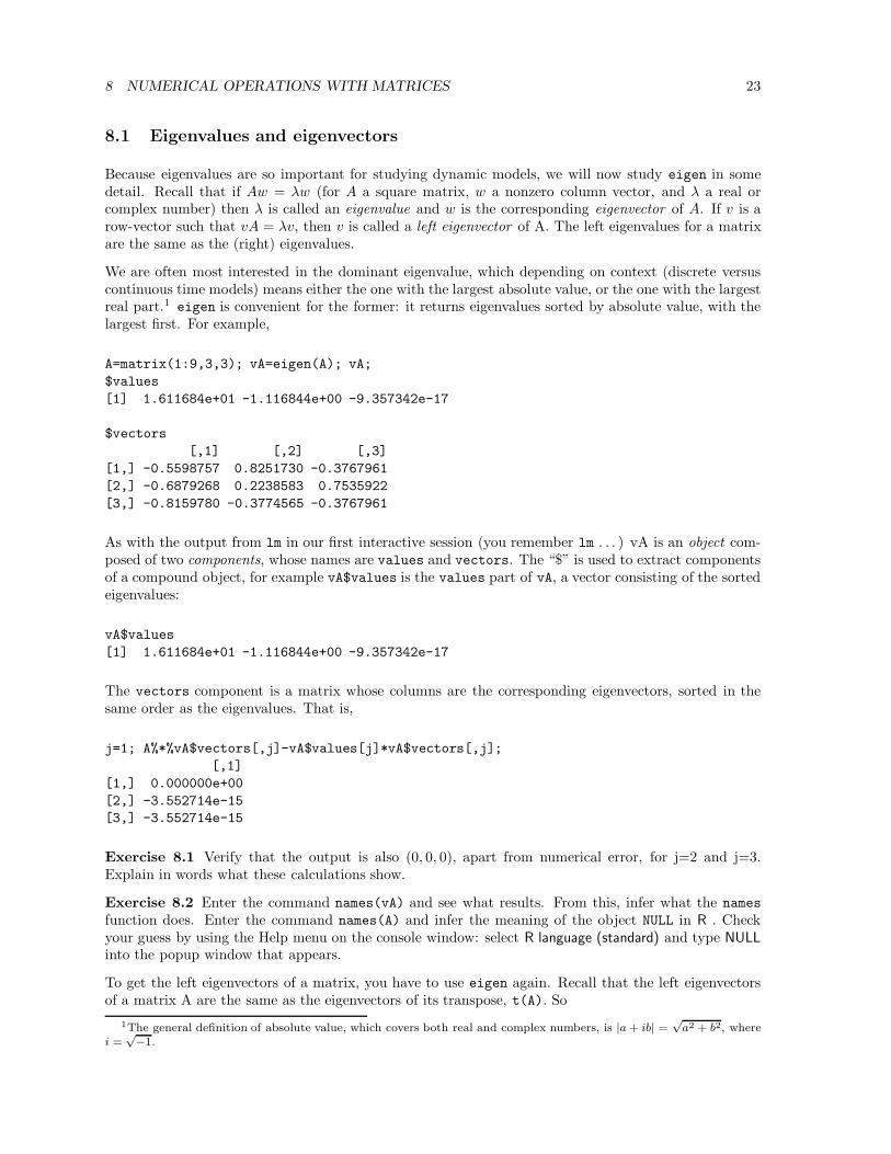
8.1 Eigenvalues and eigenvectors

Because eigenvalues are so important for studying dynamic models, we will now study eigen in somedetail. Recall that if Aw = "w (for A a square matrix, w a nonzero column vector, and " a real orcomplex number) then " is called an eigenvalue and w is the corresponding eigenvector of A. If v is arow-vector such that vA = "v, then v is called a left eigenvector of A. The left eigenvalues for a matrixare the same as the (right) eigenvalues.

We are often most interested in the dominant eigenvalue, which depending on context (discrete versuscontinuous time models) means either the one with the largest absolute value, or the one with the largestreal part.1 eigen is convenient for the former: it returns eigenvalues sorted by absolute value, with thelargest first. For example,

A=matrix(1:9,3,3); vA=eigen(A); vA;$values[1] 1.611684e+01 -1.116844e+00 -9.357342e-17

$vectors[,1] [,2] [,3]

[1,] -0.5598757 0.8251730 -0.3767961[2,] -0.6879268 0.2238583 0.7535922[3,] -0.8159780 -0.3774565 -0.3767961

As with the output from lm in our first interactive session (you remember lm . . . ) vA is an object com-posed of two components, whose names are values and vectors. The “$” is used to extract componentsof a compound object, for example vA$values is the values part of vA, a vector consisting of the sortedeigenvalues:

vA$values[1] 1.611684e+01 -1.116844e+00 -9.357342e-17

The vectors component is a matrix whose columns are the corresponding eigenvectors, sorted in thesame order as the eigenvalues. That is,

j=1; A%*%vA$vectors[,j]-vA$values[j]*vA$vectors[,j];[,1]

[1,] 0.000000e+00[2,] -3.552714e-15[3,] -3.552714e-15

Exercise 8.1 Verify that the output is also (0, 0, 0), apart from numerical error, for j=2 and j=3.Explain in words what these calculations show.

Exercise 8.2 Enter the command names(vA) and see what results. From this, infer what the namesfunction does. Enter the command names(A) and infer the meaning of the object NULL in R . Checkyour guess by using the Help menu on the console window: select R language (standard) and type NULLinto the popup window that appears.

To get the left eigenvectors of a matrix, you have to use eigen again. Recall that the left eigenvectorsof a matrix A are the same as the eigenvectors of its transpose, t(A). So

1The general definition of absolute value, which covers both real and complex numbers, is |a + ib| =!

a2 + b2, wherei =

!"1.


vLA=eigen(t(A))$vectorsgets you the left eigenvectors of A.

Exercise 8.3 Compute vLA[,j]%*%A-vA$values[j]*vLA[,j] to verify the last claim about left eigen-vectors, for j=1 to 3.

Eigenvector scalings: For a transition matrix model, the dominant right eigenvector w (i.e. theeigenvector corresponding to the eigenvalue with largest absolute value) is the stable stage distribution, sowe are most interested in relative proportions. To get those, w=w/sum(w). The dominant left eigenvectorv is the reproductive value, and it is conventional to scale those relative to the reproductive value of anewborn. If newborns are class 1: v=v/v[1].

Exercise 8.4 : Write a script file which applues the above to the matrices

A =

#

$1 #5 06 4 00 0 2

%

& B =

#

$0 1 5

0.6 0 00 0.4 0.9

%

&

finding all the eigenvalues and then extracting the dominant one and the corresponding left and righteigenvectors. For B, use the scalings defined above.

8.2 Eigenvalue sensitivities and elasticities

For an n % n matrix A with entries aij, the sensitivities sijand elasticities eijcan be computed as

sij =#"

#aij=

viwj

(v, w) eij =aij

"sij (1)

where " is the dominant eigenvalue, v and w are dominant left and right eigenvalues, and (v, w) is theinner product of v and w, computed in R as sum(v*w). So once ", v, and w have been found andstored as variables, it just takes some for-loops to compute the sensitivies and elasticities.

vA=eigen(A); lambda=vA$values[1];w=vA$vectors[,1]; w=w/sum(w);v=eigen(t(A))$vectors[,1]; v=v/v[1];vdotw=sum(v*w);s=A; n=dim(A)[1];for(i in 1:n) {

for(j in 1:n) {s[i,j]=v[i]*w[j]/vdotw;

}}e=(s*A)/lambda;

Note how all the elasticities are computed at once in the last line. In R that kind of “vectorized”calculation is much quicker than computing entries one-by-one in a loop. Even better is to use a built-in function that operates at the vector or matrix level. In this case we can use outer to completelyeliminate the nested do-loops:

vA=eigen(A); lambda=vA$values[1];w=vA$vectors[,1]; w=w/sum(w);v=eigen(t(A))$vectors[,1]; v=v/v[1];


s=outer(v,w)/sum(v*w);e=(s*A)/lambda;

Vectorizing code to avoid or minimize loops is an important aspect of e"cient R programming.

Exercise 8.5 Construct the transition matrix A, and then find ", v, w for an age-structured modelwith the following survival and fecundity parameters.

Age-classes 1-6 are genuine age classes with survival probabilities (p1p2 · · ·p6) = (0.3, 0.4, 0.5, 0.6,0.6, 0.7)

Note that pj = aj+1,j, the chance of surviving from age j to age j + 1, for these ages. You can create avector p with the values above and then use a for-loop to put those values into the right places in A.

Age-class 7 are adults, with survival 0.9 and fecundity 12.

Results: " = 1.0419

A =

#

''''''''$

0 0 0 0 0 0 12.3 0 0 0 0 0 00 .4 0 0 0 0 00 0 .5 0 0 0 00 0 0 .6 0 0 00 0 0 0 .6 0 00 0 0 0 0 .7 .9

%

((((((((&

w = (0.6303, 0.1815, 0.0697, 0.0334,0.0193,0.0111)v = (1, 3.4729, 9.0457, 18.8487,32.7295, 56.8328,84.5886)

8.3 Finding the eigenvalue with largest real part

For the Jacobian matrix of a di!erential equation model, the dominant eigenvalue is the one with thelargest real part. To find this, and the associated eigenvector, we need to extract the real parts of theeigenvalues and locate the largest one.

Use the help system – (?complex) – to see the R functions for working with complex numbers. The onewe need now is Re, which extracts the real parts of complex numbers.

Use data.entry to create the matrix

A =

#

$3 0 02 2 #30 3 1

%

&

and you should find that eigen(A)$values are[1] 1.5+2.95804i 1.5-2.95804i 3.0+0.00000i.

The first two are a complex conjugate pair with absolute value 3.316625 (mod(eigen(A)$values) getsyou the absolute values of the eigenvalues), but the third one has the largest real part.

To have R do this for you, we use the which function to find where the real part is maximized.

vA=eigen(A)$values; rmax=max(Re(vA));j=which(vA==rmax);lmax=vA[j]; vmax=eigen(A)$vectors[,j];

The first line uses max to compute the largest real part of any eigenvalue. In the second line, which findsthe indices at which the logic condition (vA==rmax) are TRUE, in this case j=3. The third line thenextracts the relevant entries from the lists of eigenvalues and eigenvectors.

9 CREATING NEW FUNCTIONS 26

Exercise 8.6 Try the above on A=diag(3,1,3) and see what you get for lmax and vmax. Why?

9 Creating new functions

Functions (often called subroutines in other computing languages) allow you to break a program intosubunits. This makes complex problems easier to program, and helps us (and others) to understand thelogical flow of programs. Each function is an independent little program, performing one task or a fewrelated tasks, and returning the results. A program can then be written to call on various functions toperform di!erent tasks. Each function can be written and tested independently, which leads naturallyto the generally recommended modular style of program construction.

The basic syntax for creating a function is as follows. Suppose [for the sake of an easy example] youwant a function mysquare that produces sums of squares: given vectors v and w, it returns a vectorconsisting of the element-by-element sums of the squares of the elements in the two vectors. The syntaxfor doing that is as follows:

mysquare=function(v,w) {u=v^2+w^2;return(u)

}

This code e!ectively adds mysquare as a new R command, just like sin or log. The variable u is internalto the function; if you use mysquare in a program, the program won’t “know” the value of u.

Exercise 9.1 Type the above into a script file and run it, and then do q=mysquare(1:4,1:4); q inthe console window.

Schematically,

function.name=function(argument1,argument2,...) {command;command;

...command;return(value)

}

Functions can be placed anywhere in a script file. Once the code for a function has been executed withina session, the new function can be treated like any other R command.

Functions can return several di!erent values, by combining them into a list with named parts.

mysquare2=function(v,w) {q=v^2; r=w^2return(list(v.squared=q,w.squared=r))

}

You can then extract the components in the usual way.

> x=mysquare2(1:4,2:5); names(x);[1] "v.squared" "w.squared"

10 A SIMULATION PROJECT 27

> x$v.squared[1] 1 4 9 16

Exercise 9.2 Write a function domeig that takes as input a single vector, and returns a list withcomponents average (mean of the values in the vector), and variance (the variance of the values in thevector).

10 A simulation project

This section is an optional “capstone” project putting into use the programming skills that have beencovered so far. Nothing new about R per se is covered in this section.

The first step is to write a script file that simulates a simple model for density-independent populationgrowth with spatial variation. The model is as follows. The state variables are the numbers of individualsin a series of L = 20 patches along a line (L stands for “length of the habitat”) .

1 2 3 4 ... ... L-1 L

Let Nj(t) denote the number of individuals in patch j (j = 1, 2, . . . , L) at time t (t = 1, 2, 3, . . . ), and let"j be the geometric growth rate in patch j. The dynamic equations for this model consist of two steps:

1. Geometric growth within patches:

Mj(t) = "jNj(t) for all j. (2)

2. Dispersal between neighboring patches:

Nj(t + 1) = (1 # 2d)Mj(t) + dMj!1(t) + dMj+1(t) for 2 * j * L # 1 (3)

where 2d is the “dispersal rate”. We need special rules for the end patches. For this exercise weassume reflecting boundaries: those who venture out into the void have the sense to come back.That is, there is no leftward dispersal out of patch 1 and no rightward dispersal out of patch L:

N1(t + 1) = (1 # d)M1(t) + dM2(t)NL(t + 1) = (1 # d)ML(t) + dML!1(t)

(4)

• Write your script to start with 5 individuals in each patch at time t=1, iterate the model up to t=50,and graph the log of the total population size (the sum over all patches) over time. Use the followinggrowth rates: "j = 0.9 in the left half of the patches, and "j = 1.2 in the right.• Write your program so that d and L are parameters, in the sense that the first line of your script filereads d=0.1; L=20; and the program would still work if these were changed other values.

Notes and hints:

1. This is a real programming problem. Think first, then start writing your code.

2. Notice that this model is not totally di!erent from Loop1.m, in that you start with a foundingpopulation at time 1, and use a loop to compute successive populations at times 2,3,4, and so on.The di!erence is that the population is described by a vector rather than a number. Therefore, tostore the population state at times t = 1, 2, · · · , 50 you will need a matrix njt with 50 rows and Lcolumns. Then njt(t,:) is the population state vector at time t.

11 COIN TOSSING AND MARKOV CHAINS 28

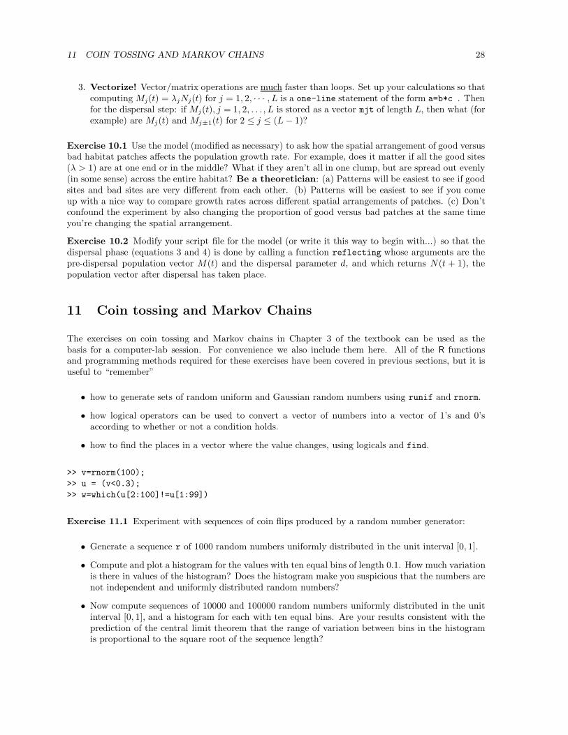
3. Vectorize! Vector/matrix operations are much faster than loops. Set up your calculations so thatcomputing Mj(t) = "jNj(t) for j = 1, 2, · · · , L is a one-line statement of the form a=b*c . Thenfor the dispersal step: if Mj(t), j = 1, 2, . . . , L is stored as a vector mjt of length L, then what (forexample) are Mj(t) and Mj±1(t) for 2 * j * (L # 1)?

Exercise 10.1 Use the model (modified as necessary) to ask how the spatial arrangement of good versusbad habitat patches a!ects the population growth rate. For example, does it matter if all the good sites(" > 1) are at one end or in the middle? What if they aren’t all in one clump, but are spread out evenly(in some sense) across the entire habitat? Be a theoretician: (a) Patterns will be easiest to see if goodsites and bad sites are very di!erent from each other. (b) Patterns will be easiest to see if you comeup with a nice way to compare growth rates across di!erent spatial arrangements of patches. (c) Don’tconfound the experiment by also changing the proportion of good versus bad patches at the same timeyou’re changing the spatial arrangement.

Exercise 10.2 Modify your script file for the model (or write it this way to begin with...) so that thedispersal phase (equations 3 and 4) is done by calling a function reflecting whose arguments are thepre-dispersal population vector M (t) and the dispersal parameter d, and which returns N (t + 1), thepopulation vector after dispersal has taken place.

11 Coin tossing and Markov Chains

The exercises on coin tossing and Markov chains in Chapter 3 of the textbook can be used as thebasis for a computer-lab session. For convenience we also include them here. All of the R functionsand programming methods required for these exercises have been covered in previous sections, but it isuseful to “remember”

• how to generate sets of random uniform and Gaussian random numbers using runif and rnorm.

• how logical operators can be used to convert a vector of numbers into a vector of 1’s and 0’saccording to whether or not a condition holds.

• how to find the places in a vector where the value changes, using logicals and find.

>> v=rnorm(100);>> u = (v<0.3);>> w=which(u[2:100]!=u[1:99])

Exercise 11.1 Experiment with sequences of coin flips produced by a random number generator:

• Generate a sequence r of 1000 random numbers uniformly distributed in the unit interval [0, 1].

• Compute and plot a histogram for the values with ten equal bins of length 0.1. How much variationis there in values of the histogram? Does the histogram make you suspicious that the numbers arenot independent and uniformly distributed random numbers?

• Now compute sequences of 10000 and 100000 random numbers uniformly distributed in the unitinterval [0, 1], and a histogram for each with ten equal bins. Are your results consistent with theprediction of the central limit theorem that the range of variation between bins in the histogramis proportional to the square root of the sequence length?


Note: q=hist(runif(1000),10) will plot the first histogram you need, and q$counts will hold thenumber in each bin of the histogram.

Exercise 11.2 Convert the sequence of 1000 random numbers r from the previous exercise into asequence of outcomes of coin tosses in which the probability of heads is 0.6 and the probability of tailsis 0.4. Then,

• Recall that this coin tossing experiment is modeled by the binomial distribution: the probabilityof k heads in the sequence is given by

ck(0.6)k(0.4)1000!k where ck =)

1000k

*=

1000!k!(1000# k)!

.

In R , choose(n,k) computes the binomial coe"cient)

nk

*.

Calculate the probability of k heads for values of k between 500 and 700 in a sequence of 1000independent tosses. Plot your results with k on the x-axis and the probability of k heads on they-axis. Comment on the shape of the plot.

• Now test the binomial distribution by doing 1000 repetitions of the sequence of 1000 coin tossesand plot a histogram of the number of heads obtained in each repetition. Compare the resultswith the predictions from the binomial distribution.

• Repeat this experiment with 10000 repetitions of 100 coin tosses. Comment on the di!erences youobserve between this histogram and the histogram for 1000 repetitions of tosses of 1000 coins.

Tossing multi-sided coins Uniform random numbers can also be used to simulate “coin-toss” experi-ments where the coin has 3 or more sides. Conceptually this is easy. If there are n sides with probabilitiesp1, p2, · · · , pn, you generate r=runif(1) and declare that

Side 1 occurs if r * p1.

Side 2 occurs if p1 < r * p1 + p2

Side 3 occurs if p1 + p2 < r * p1 + p2 + p3

· · ·

Side n occurs if p1 + p2 + · · ·+ pn!1 < r.

To code this compactly in R , note that the outcome depends on the cumulative sums

c1 = p1, c2 = p1 + p2, c3 = p1 + p2 + p3, · · · , cn = 1.

If r is larger than exactly k of these, then the outcome is Side k + 1. Cumulative sums of a vector arecomputed using the function cumsum.

As an example, the following code tosses a 5-sided coin with probabilities given by the vector p definedin the first line:

p=c(.3,.1,.3,.1,.2); b=cumsum(p);side=sum(runif(1)>b)+1

To toss the coin repeatedly you can use the sapply function, which applies an arbitrary function to allelements in a vector.


side=sapply(runif(1000),FUN=function(x) sum(x>b)+1)

In the code above the function to be applied is defined within the call to sapply. More complicatedfunctions can be defined separately, prior to the call, as in the following example:

side.choose=function(x) {sum(x>b) +1}side=sapply(runif(1000),FUN=side.choose)

Exercise 11.3 Generate 10000 tosses of a 3-sided coin (with your choice of probabilities), and plot ahistogram of the results to verify that your coin is behaving the way it should.

11.1 Markov chains and residence times

The purpose of the following exercises is to generate synthetic data for single channel recordings fromfinite state Markov chains, and to explore patterns in the “data”. Single channel recordings give thetimes that a Markov chain makes a transition from a closed to an open state or vice versa. The histogramof expected residence times for each state in a Markov chain is exponential, with di!erent mean residencetime for di!erent states. To observe this in the simplest case, we again consider coin tossing. The twooutcomes, heads or tails, are the di!erent states in this case. Therefore the histogram of residence timesfor heads and tails should each be exponential. The following steps are taken to compute the residencetimes:

• Generate sequences of independent coin tosses based on given probabilities.

• Look at the number of transitions that occur in each of the sequences (a transition is when twosuccessive tosses give di!erent outcomes).

• Calculate the residence times by counting the number of tosses between each transition.

Exercise 11.4 Find the script cointoss.R. This program calculates the residence times of coin tossesby the above methodology. Are the residence times consistent with the prediction that their histogramdecreases exponentially? Produce a plot that compares the predicted results with the simulated residencetimes stored by cointoss.R in the vectors hhist and thist. (Suggestion: use a logarithmic scale forthe values with the matlab command semilogy.)

Models for stochastic switching among conformational states of membrane channels are somewhat morecomplicated than the coin tosses we considered above. There are usually more than 2 states, andthe transition probabilities are state dependent. Moreover, in measurements some states cannot bedistinguished from others. We can observe transitions from an open state to a closed state and viceversa, but transitions between open states (or between closed states) are “invisible”. Here we shallsimulate data from a Markov chain with 3 states, collapse that data to remove the distinction between 2of the states and then analyze the data to see that it cannot be readily modeled by a Markov chain withjust two states. We can then use the distributions of residence times for the observations to determinehow many states we actually have.

Suppose we are interested in a membrane current that has three states: one open state, O, and twoclosed states, C1 and C2. As in the kinetic scheme discussed in class, state C1 cannot make a transitionto state O and vice-versa. We assume that state C2 has shorter residence times than states C1 or O.Here is the transition matrix of a Markov chain we will use to simulate these conditions:

C1 C2 O+

,.98 .1 0.02 .7 .050 .2 .95

-

.C1

C2

O

12 THE HODGKIN-HUXLEY MODEL 31

You can see from the matrix that the probability 0.7 of staying in state C2 is much smaller than theprobability 0.98 of staying in state C1 or the probability 0.95 of remaining in state O.

Exercise 11.5 Generate a set of 100000 samples from the Markov chain with these transition proba-bilities. We will label the state C1 by 1, the state C2 by 2 and the state O by 3. This can be done bya modification of the method that we used to toss coins with 3 or more sides. The modification is thatthe probabilities of each side depend on the current state of the membrane:

nt = 100000;A = matrix(c(0.98, 0.10, 0, 0.02, 0.7, 0.05, 0, 0.2, 0.95),3,3,byrow=T);B = apply(A,2,cumsum); #cumulative sums of each columnA; B;states=numeric(nt+1); rd=runif(nt);states[1] = 3; # Start in open statefor(i in 1:nt) {

b=B[,states[i]]; #cumulative probabilities for current statestates[i+1]=sum(rd[i]>b)+1 # do the ‘‘coin toss’’ based on current state

}plot(states[1:1000],type="s");

Notice the use of apply to compute the cumulative sum of each column of the transition matrix, andtype="s" to get a “stairstep” plot of the state transitions (see ?plot).

Exercise 11.6 Compute the eigenvalues and eigenvectors of the matrix A. Compute the total time thatyour “data” in the vector states spends in each state (use vector operations to do this!) and comparethe results with predictions coming from the dominant right eigenvector of A.

Exercise 11.7 Produce a new vector rstates by “reducing” the data in the vector states so thatstates 1 and 2 are indistinguishable. The states of rstates will be called “closed” and “open”.

Exercise 11.8 Plot histograms of the residence times of the open and closed states in rstates byapplying the methods used in the script cointoss.R. Comment on the shapes of the distributions ineach case. Using your knowledge of the transition matrix A, make a prediction about what the residencetime distributions of the open states should be. Compare this prediction with the data. Show that theresidence time distribution of the closed states is not fit well by an exponential distribution.

12 The Hodgkin-Huxley model

The purpose of this section is to develop an understanding of the components of the Hodgkin-Huxleymodel for the membrane potential of a space-clamped squid giant axon. It goes with the latter part ofChapter 3 in the textbook, and with the Recommended reading: Hille, Ion Channels of ExcitableMembranes, Chapter 2.

The Hodgkin-Huxley model is the system of di!erential equations

Cdv

dt= i #

/gNam3h (v # vNa) + gKn4 (v # vK) + gL (v # vL)

0

dm

dt= 3

T!6.310

1(1 # m)#

)#v # 35

10

*# 4m exp

)#v # 60

18

*2

dn

dt= 3

T!6.310

10.1 (1 # n)#

)#v # 50

10

*# 0.125n exp

)#v # 60

80

*2

dh

dt= 3

T!6.310

10.07(1 # h) exp

)#v # 60

20

*# h

1 + exp(#0.1(v + 30))

2


where#(x) =

x

exp(x) # 1.

The state variables of the model are the membrane potential v and the ion channel gating variables m,n, and h, with time t measured in msec. Parameters are the membrane capacitance C, temperature T ,conductances gNa, gK, gL, and reversal potentials vNa, vK , vL. The gating variables represent channelopening probabilities and depend upon the membrane potential. The parameter values used by Hodgkinand Huxley are:

gNa gK gL vNa vK VL T C120 36 0.3 55 -72 -49.4011 6.3 1

Most of the data used to derive the equations and the parameters comes from voltage clamp experimentsof the membrane, e.g Figure 2.7 of Hille. In this set of exercises, we want to see that the model reproducesthe voltage clamp data well, and examine some of the approximations and limitations of the parameterestimation.

When the membrane potential v is fixed, the equations for the gating variables m, n, h are first orderlinear di!erential equations that can be rewritten in the form

$xdx

dt= #(x # x")

where x is m, n or h.

Exercise 12.1 Re-write the di!erential equations for m, n, and h in the form above, thereby obtainingexpressions for $m, $n, $h and minf , ninf , hinf as functions of v.

Exercise 12.2 Write an R script that computes and plots $m, $n, $h and minf , ninf , hinf as functions ofv for v varying from #100mV to 75mV. You should obtain graphs that look like Figure 2.17 of Hille.

In voltage clamp, dvdt = 0 so we obtain the following formula for the current from the Hodgkin-Huxley

model:i = gNam3h(v # vNa) + gKn4(v # vK) + gL(v # vL)

The solution of the first order equation

$xdx

dt= #(x # x")

isx(t) = x" + (x(0) # x") exp(

#t

$x)

Exercise 12.3 Write an R script to compute and plot as a function of time the current i(t) obtainedfrom voltage clamp experiments in which the membrane is held at a potential of #60mV and thenstepped to a higher potential vs for 6msec. (When the membrane is at its holding potential #60mV, thevalues of m, n, h approach m"(#60), n"(#60), h"(#60). Use these approximations as starting values.)As in Figure 2.7 of Hille, use vs = #30,#10, 10, 30,50,70,90 and plot each of the curves of current onthe same graph.

Exercise 12.4 Separate the currents obtained from the voltage clamp experiments by plotting onseparate graphs each of the sodium, potassium and leak currents.

Exercise 12.5 Hodgkin and Huxley’s 1952 papers explain their choice of the complicated functionsin their model, but they had no computers available to analyze their data. In this exercise and the


next, we examine procedures for estimating from experimental data the sodium current parametersm", h", $m, $h. However, the data that we will use will be generated by the model itself: as in Exercises2 and 3 compute the Hodgkin-Huxley sodium current generated by a voltage clamp experiment with aholding potential of #90mV and steps to vs = #80,#70,#60,#50,#40,#30,#20,#10, 0. This is your“data”.2 Using the expression gNam3h(v # vNa) for the sodium current, estimate m", $m, h" and$h as functions of voltage from this simulated data. The most commonly used methods assume that$m is much smaller than $h, so that the activation variable m reaches its steady state before h changesmuch. Explain the procedures you use. Some of the parameters are di"cult to determine, especially overcertain ranges of membrane potential. Why? How do your estimates compare with the values computedin Exercise 1?

Challenge: For the parameters that you had di"culty estimating in Exercise 4, simulate voltage clampprotocols that help you estimate these parameters better. (See Hille, pp. 44-45.) Describe the protocolsand how you estimate the parameters. Plot the currents produced by the model (as in Exercise 2) foryour new experiments, and give the parameter estimates that you obtain using the additional “data”from your experiments. Further investigation of these procedures is a good topic for a course project!

12.1 Getting started

We o!er here some suggestions for completing the exercises in this section.

Complicated expressions are often built by composing simpler expressions. In any programming lan-guage, it helps to introduce intermediate variables. Here, let’s look at the gating variable h first. Wehave

dh

dt= 0.07 exp

)#v # 60

20

*(1 # h) # h

1 + exp(#0.1(v + 30)Introduce the intermediate expressions

ah = 0.07 exp)#v # 60

20

*

andbh =

11 + exp(#0.1(v + 30)

.

Thendh

dt= ah(1 # h) # bhh = ah # (ah + bh)h.

We can then divide this equation by (ah + bh) to obtain the desired form

$hdh

dt= #(h # h")

as1

ah + bh

dh

dt=

ah

ah + bh# h.

Comparing these two expressions we have

$h =1

ah + bh, h" =

ah

ah + bh.

Implementing this in R to compute the values of h"(#45) and $h(#45), we write2Analyzing data that come from a model to estimate parameters that you already know may sounds a bit crazy at first,

but statisticians do this all the time and many of them are not crazy. Before trying to fit a model to real data, it’s a goodidea to generate artificial “data” using the model with known parameters, and make sure that your approach to fitting themodel allows you to recover the parameters that generated the “data”.


v = -45;ah = 0.07*exp((-v-60)/20);bh = 1/(1+exp(-0.1*(v+30)));tauh = 1/(ah+bh);hinf = ah/(ah+bh);

Evaluation of this script gives tauh = 4.6406 and hinf = 0.1534.

To do the second exercise, for th and h", we want to evaluate the script for values of v that vary from-100 to 75. We will do this at integer values of v with a loop. We first make vectors to hold the data,and then store each value as it is computed:

tauh = rep(0,176); # to start with v = -100, end with v = 75hinf = rep(0,176);

for(j in 1:176){v = -101+j; # so v goes from -100 to 75ah = 0.07*exp((-v-60)/20);bh = 1/(1+exp(-0.1*(v+30)));tauh(j) = 1/(ah+bh);hinf(j) = ah/(ah+bh);

}

The same strategy can be used to compute m", $m, n", $n, but there is one slight twist: the function#. This function defined by

#(x) =x

exp(x) # 1

gives the indeterminate value 0/0 when x = 0, so R cannot evaluate it there. Nonetheless, usingl’Hopital’s rule from calculus, we can define #(0) = 1. When computing the values in R , either avoidx = 0 or use an if statement to check whether x = 0. It is helpful in writing R scripts to compute theterms involving # to introduce intermediate variables for its argument:

...amv = -(v+35.0)/10.0;am = amv/(exp(amv) - 1);...

You will need some of the data from the second exercise in completing the third and fourth, and youshould extend the range of v to include v = 90 for these exercises. It is helpful to define the parameters,a vector t of the time values that you want to use in computing the currents, values of m, n, h at theholding potential v = #60, values of m", n", h" and $m, $n, $h at the potentials of the steps, arrays thatwill hold all of the data for each of the gating variables m, n, h, etc. before you compute the currents.Use code like m[s,j] = m1[s] + (m0 - m1[s])*exp(-t[j]/mt1[s]) to compute the gating variables,with m0 the value of m at the holding potential, m1[s] the value of m" during the step and mt1[s] thevalue of $m during the step. Once these arrays have been computed, use

i = gNam3h(v # vNa) + gKn4(v # vK) + gL(v # vL)

to compute the total current, with gNam3h(v#vNa) and gKn4(v#vK ) giving the sodium and potassiumcurrents.

The fifth exercise requires much more ingenuity than the previous ones. To get started, repeat compu-tations like those of Exercise 3 to generate the sodium current data used in the exercise. Currents must

13 SOLVING SYSTEMS OF DIFFERENTIAL EQUATIONS 35

be converted to conductances by dividing by (v # vNa). After this is done, strategies must be developedto estimate m", h", $m, $h. Frequently used procedures assume that

1. the experiment starts at a potential su"ciently hyperpolarized that there is no inactivation (i.e.h = 1) and

2. activation is so fast relative to inactivation that m reaches its steady state before h has changedsignificantly.

This separation of time scales – m changing much faster than h because $m + $h – means that early,rapid changes in conductance are caused by changes in m, while later, slower changes in conductanceare caused by changes in h. One can then estimate m" and $m from the increasing portion of theconductance traces, assuming that h = 1 during this entire period of time, so that the conductance isgNam3. Then to estimate $h we assume that the decreasing “tail” of the conductance curve is given bygNam3

"h(t), because m(t) has already converged to its steady state.

It is easier to estimate h" from a di!erent set of voltage traces, having di!erent values of the holdingpotential v0, followed by a step to another potential v1 that is the same for each trace. In this protocolwe start with h partially inactivated (i.e. h < 1), so the peak conductance during the subsequent traceis proportional to the initial value of h, which is h"(v0). A plot of peak conductance as a function of v0

is then proportional to a plot of h" as a function of v0. The constant of proportionality can be inferredfrom the fact that the maximum value of h"(v) is 1. Consult Hille for further descriptions of theseprotocols.

13 Solving systems of di!erential equations

R built-in functions make it relatively easy to do some complicated things. One important example isfinding numerical solutions for a system of di!erential equations

dx

dt= f(t, x).

Here x is a vector assembled from quantities that change with time, and the vector field f gives theirrates of change. The Hodgkin-Huxley model from the last section is one example. Here we start with asimple model of a gene regulation network from the paperT. Gardner, C. Cantor and J. Collins. Construction of a genetic toggle switch in Escherichia coli. Nature403: 339-342.The model (described more fully in the textbook) is

du

dt= #u +

%u

1 + v!

dv

dt= #v +

%v

1 + u"

(5)

The variables u, v in this system are functions of time. They represent the concentrations of two repressorproteins Pu, Pv in bacteria that have been infected with a plasmid containing genes that code for Pu andPv. The plasmid also contains promoters, with Pu a repressor of the promoter of the gene coding for Pv

and vice-versa.

The equations are a simple “bathtub” model describing the rates at which u and v change with time.Pu is degraded at the rate u and is produced at a rate #u

1+v! , which is a decreasing function of v. Theexponent & models the “cooperativity” in the repression of Pu synthesis by Pv. These two processes of

degradation and synthesis combine to give the equation fordu

dt, and the equation for

dv

dtis similar.


There are no explicit formulas to solve this pair of equations, but we can interpret what the equationsmean geometrically. At each point of the (u, v) plane, we regard (du

dt , dvdt ) as a vector that gives the

direction and magnitude for how fast (u, v) jointly change as a function of t. Solutions to the equationsgive rise to parametric curves (u(t), v(t)) whose tangent vectors (du

dt , dvdt ) are those specified by the

equations.

To plot the vector field, first run the script DMBpplane.R (this script is based on pplane.R by DanielKaplan, Department of Mathematics, Macalester College, and has been modified and used here withhis permission). This script includes a function that computes the vector field for model (5) with theassumption that %u = %v:

toggle=function(u,v,parms) {du= -u + parms[1]/(1+v^parms[2]);dv= -v + parms[1]/(1+u^parms[3]);return(c(du,dv));

}

Note how this function is set up:

• Its input arguments are the two state variables u,v and a parameter vector parms. Even if parmsis not used by the function, it must be included in the list of arguments.

• The function returns the vector field as a vector.

• The computations are set up so they will go through if u and v are matrices of equal size.

Use this setup for any vector field that you want to study using the functions in DMBpplane.R.

The function phasearrows (also in DMBpplane.R) can then be used to plot the vector field, as in thisexample:

phasearrows(fun=toggle,xlim=c(0,3),ylim=c(0,3),resol=25,parms=c(3,2,2))

In this statement, fun is the name of the function that calculates the vector field, xlim and ylim definethe range of values for the plot, and setting resol=25 means that arrows showing the vector field willbe drawn at a 25%25 grid of points within the plotting region. The parameter vector parms is passed tothe vector field function – this argument can be omitted if the vector field function does not use parms.

Exercise 13.1 Run DMBpplane.R to create the toggle function, and then use the command aboveto plot the vector field.

We can think of solutions to (5) as curves in the plane that “follow the arrows”. Given a startingpoint (u0, v0), the mathematical theory discussed in the textbook proves that there is a unique solution(u(t), v(t)) with (u(0), v(0)) = (u0, v0). The process of finding the solution numerically is called numer-ical integration. Methods for numerical integration build up an approximate solution by adding shortsegments of an approximate solution curve, one after another.

R ’s numerical ODE solvers are in the odesolve package. Download this (if necessary) from CRAN, andthen use the command library(odesolve) to load it into your R session.

Exercise 13.2 After you load the odesolve library, and use ?rk4 to look at the syntax for this function.

To use R ’s ODE solvers, the first step is to write a function to evaluate the vector field in the specificformat required by the solvers. Here’s what that looks like for the toggle switch model:


Toggle=function(t,y,parms) {u=y[1]; v=y[2];du= -u + parms[1]/(1+v^parms[2]);dv= -v + parms[1]/(1+u^parms[3]);dY=c(du,dv);return(list(dY));

}

There’s a bit to digest in that. Here are the things to note:

1. The function must have input arguments (t,y,parms), even if only the state vector y is used tocompute the vector field. Here t is time, y is the state vector, and

2. parms is again a vector of parameter values for the function. This allows you to see how solutionschange as parameters are varied, without having to re-write and re-run the function. It alsosimplifies the process of fitting di!erential equations to data.

3. The vector field value has to be returned as a list. There’s a good reason for this; if you’re curiousand have way too much free time on your hands, ?lsoda gives the explanation. You’ve beenwarned.

The “basic” ODE solver in R is rk4, which implements the 4th-order Runge Kutta method with a fixedtime step. The format is

out=rk4(x0,times,func,parms)

Here times is a vector of the times at which you want solution values, x0 is the value of the state vectorat the initial time (i.e. times[1]), func func is the function specifying the model (such as Toggle), andparms is the vector of parameter values that will be passed to func.

Here is an example using our Toggle function:

x0=c(.2,.1); times=seq(0,50,by=0.2); parms=c(3,2,2);out=rk4(x0,times,Toggle,parms)matplot(out[,1],out[,2:3],type="l",ylim=c(0,3),xlab="time t",ylab="u,v");

Exercise 13.3 Write a script toggle.R with the commands above, and run them to see some solutiontrajectories as a function of time. Which plotted curve is u, and which is v? How do you know? Lookat the matrix out to see how it is set up: the first column is a list of times, and the other columns arethe computed (approximate) values of the state variables at each time.

The state trajectories both seem to be approaching constants, and that these constants have di!erentvalues. A second way of looking at the trajectories (Exercise: do this yourself right now) is:

plot(out[,2],out[,3],type="l",xlab="u",ylab="v")

This kind of plot is called a phase portrait. It shows the path in the (u, v) phase plane taken by thetrajectory, but we lose track of the times at which the trajectory passes through each point on this path.

Exercise 13.4 Use rk4 again with initial conditions (0.2, 0.3) to produce a new output matrix out2and plot phase portraits of both solutions. Do this first for time interval [0, 50] and again for [0, 200].

The trajectories appear to end at the same places, indicating that they didn’t go anywhere after t = 50.We can explain this by observing that the di!erential equations vanish at these endpoints. The curves


where dudt = 0 and dv

dt = 0 are called nullclines for the vector field. They intersect at equilibriumpoints, where both du

dt = 0 and dvdt = 0. The solution with initial point an equilibrium is constant. Here,

the equilibrium points are (asymptotically) stable, meaning that trajectories close to the equilibriaapproach them as t increases.

Nullclines for a general vector field can be plotted using the function nullclines in DMBpplane.R. Thesyntax is the same as to phasearrows, for example:

nullclines(fun=toggle,xlim=c(0,3),ylim=c(0,3),resol=250,parms=c(3,2,2))

It is a good idea to use a large value of resol so that the nullclines are found accurately.

Exercise 13.5 Without erasing the nullclines, add to that plot (using points) the two solution trajec-tories with di!erent initial conditions that you have computed (out and out2 from previous exercises).You should see that each trajectory converges onto an equilibrium point where the nullclines intersect.

Exercise 13.6 There is a third equilibrium point where the two nullclines intersect, in addition to thetwo at the ends of the trajectories that you have computed. Experiment with di!erent initial conditions,to see if you can find any trajectories that converge onto this third equilibrium (Hint: what happens inthis model if u(0) = v(0) for these parameter values?)

Exercise 13.7 Change the value of % from 3 to 1.5. How does the phase portrait change? Plot thenullclines to help answer this question.

13.1 Always use lsoda!

The “industrial strength” solver in R is lsoda. This is a front end to a general-purpose di!erential equa-tion solver (called, oddly enough, lsoda) that was developed at Lawrence Livermore National Laboratory.The full calling format for lsoda is

lsoda(y, times, func, parms, rtol=1e-06, atol=1e-06, tcrit=NULL,jacfunc=NULL, verbose=FALSE, dllname=NULL, hmin=0, hmax=Inf)

Don’t panic. Defaults are provided for everything but the arguments required by rk4, so lsoda can becalled just like rk4:

out=lsoda(x0,times,toggle,parms=c(3,2,2))matplot(out[,1],out[,2:3],type="l",ylim=c(0,3));

Usually you can get away with doing this, and here we always will. The options rtol and atol can beused to control the accuracy that the numerical integration tries to achieve, by using smaller time steps.lsoda automatically adjusts step sizes to achieve the desired error tolerance (based on error estimatesthat it calculates), whereas rk4 always goes directly from one value in times to the next.

One key reason for using lsoda rather than rk4 is sti!ness. Di!erential equations are called sti! if theyhave some variables or combinations of variables changing much faster than others. Sti! systems requirespecial techniques and are harder to solve than non-sti! systems. The lsoda solver monitors the systemthat it is solving for signs of sti!ness, and automatically switches to a sti!-system solver when necessary.Many biological models are at least mildly sti!, so for real work you should always use lsoda ratherthan rk4. The only time to try rk4 is that if lsoda fails on your problem (returning an error messagerather than a solution matrix), you may get a clue as to the reason by trying rk4 with a very small timestep and seeing how the solutions behave (e.g., does a state variable blow up to infinity in finite time?).


Exercise 13.8 Write a script using lsoda to solve the Lotka-Volterra model

dx1/dt = x1(r1 # x1 # ax2)dx2/dt = x2(r2 # x2 # bx1)

in which the parameters r1, r2, a, b are all passed as parameters via the argument parms. Generatesolutions for the same parameter values with rk4 and lsoda, and compare the results.

Exercise 13.9 Write a script using lsoda to solve the constant population size SIR model with births,

dS/dt = µ(S + I + R) # &SI # µS

dI/dt = &SI # (' + µ)IdR/dt = 'I # µR

For parameter values µ = 1/60, ' = 25 (corresponding to a mean lifetime of 60 years, and diseaseduration of 1/25 of a year) and population size S(0)+ I(0)+R(0) = 1000000, explore how the dynamicsof the disease prevalence I(t) changes as you increase the value of & from 0.

13.2 The logs trick

In many biological models the state variables always must be non-negative, but a numerical ODE solverdoesn’t know this. If a variable decreases rapidly to near-zero values in the exact solution, a numericalapproximate solution might overshoot to a negative value, leading to nonsense. For example, if thenumber of infectives becomes negative in a standard SIR-type infectious disease model, the transmissionrate &SI becomes negative. So contacts between susceptibles and infectives still occur but their e!ectis to make the sick one become healthy, pushing I even more negative. Once a model goes down therabbit hole, it may never come back.

This problem can often be fixed by a simple trick that is often used but (to our knowledge) rarelywritten down. The trick is to transform the model onto natural log scale, solve the transformed model,and back-transform the output. This is much easier than it sounds, because of the fact that for anystate variable x(t),

d(log x(t))dt

=1

x(t)dx

dt. (6)

This means that you can compute the untransformed vector field dx/dt, and then get the tranformedvector field with a single element-by-element division. For example, here is the function that computesthe toggle-switch model vector field on log scale. The input argument logy is the log-transformed statevector (logu, logv).

Toggle.log=function(t,logy,parms) {y=exp(logy);u=y[1]; v=y[2];du= -u + parms[1]/(1+v^parms[2]);dv= -v + parms[1]/(1+u^parms[3]);dY=c(du,dv);return(list(dY/y));}

There are only two di!erences from the original Toggle: the first line that back-transforms from logy toy, and the last line that uses equation (6) to compute the vector field of the log-transformed state vector.And there are just two minor di!erences in the call to lsoda: log-transforming the initial conditions, andback-transforming the output.

14 EQUILIBRIUM POINTS AND LINEARIZATION 40

x0=log(c(.2,.1)); times=seq(0,50,by=1); parms=c(3,2,2);out=lsoda(x0,times,Toggle.log,parms);out[,-1]=exp(out[,-1]) #column 1 is time, which was not transformedmatplot(out[,1],out[,2:3],type="l",ylim=c(0,3),xlab="time t",ylab="u,v");

Exercise 13.10 Write a script to solve the Lotka-Volterra model (in the previous subsection) usingthe log trick. Note that for this model you can do (6) in your head and avoid the dY/y calculation.

14 Equilibrium points and linearization

This section continues our study of di!erential equations with R . We will investigate the computation ofequilibrium points and their linearization. Recall that an equilibrium point of the system dx

dt = f(x) is avector x0 in the phase space where f(x0) = 0. If the models state vector has dimension n, the equilibriumcondition f(x0) = 0 is a system of n equations in n variables that may have multiple solutions, or nosolutions at all.

Solving nonlinear equations is a di"cult task for which there are no sure-fire algorithms. Newton’smethod is a simple iterative algorithm that is usually very fast when it works, but it doesn’t always work.Newton’s method takes as its input a starting value of x0, ideally one that is close to the solution off(x0) = 0 that we seek. It evaluates y0 = f(x0) and terminates if the magnitude of y0 is smaller than adesired tolerance. If y0 is larger than the desired tolerance, then a new value x1 is computed from thesolution of the linear or tangent approximation to f at x0:

f(x) , L(x) = f(x0) + Df(x0)(x # x0).

Here Df(x0) is the n%n Jacobian matrix of the partial derivatives of f evaluated at x0 – the jth columnof Df is the derivative of f with respect to the jth state variable. If Df(x0) is an invertible matrix,then we can solve the linear system L(x) = 0 for x, yielding the new value of x:

x1 = x0 # [Df(x0)]!1f(x0)

. So we replace x0 by x1 and start over again by evaluating f(x1). If its magnitude is small enough, westop. Otherwise, we take x1 as our new “starting value” and repeat the process to find a point x2 thatis (hopefully) closer to being a solution of f(x) = 0.

Close to a solution of f(x) = 0 at which Df(x) is an invertible matrix, Newton’s method converges“quadratically”, meaning that the error after one additional iteration is proportional to the currenterror squared – which is a very good thing one the error has become small.

The function newton in DMBpplane.R implements Newton’s method functions set up in the format usedfor solving di!erential equations with rk4 or lsoda. So we can apply Newton’s method to our toggleswitch model (5) using the commands

newton(Toggle,x0=c(2.5,0.4),parms=c(3,2,2))

The function newton has three optional arguments for which default values are provided: the maximumnumber of iterations niter, the convergence tolerance tol, and the increment inc used to computeJacobian matrices Df by finite-di!erence approximation to the derivatives.

Exercise 14.1 Download and run DMBpplane.R, and then run the command above. Note that thevalues of the state variables are displayed at each iteration. Recall that for these parameter values thereare three equilibrium points. Choose di!erent values of x0 to find the other two equilibrium points.

The file repress.R implements the six dimensional repressilator model of Elowitz and Leibler:

14 EQUILIBRIUM POINTS AND LINEARIZATION 41

repress=function(t,y,p){dy = rep(0,6);dy[1] = -y[1] + p[1]/(1.+y[6]^p[4])+ p[2];dy[2] = -y[2] + p[1]/(1.+y[4]^p[4])+ p[2];dy[3] = -y[3] + p[1]/(1.+y[5]^p[4])+ p[2];dy[4] = -p[3]*(y[4]-y[1]);dy[5] = -p[3]*(y[5]-y[2]);dy[6] = -p[3]*(y[6]-y[3]);return(list(dy))

}

Note that to save typing parms is replaced here by p – the name doesn’t matter so long as it’s in theright place in the list of arguments.

Exercise 14.2 Use lsoda and repress to reproduce the textbook figure that shows oscillations in thismodel by computing and graphing a trajectory for this model with parameters parms = c(50,0,0.2,2).Almost any initial conditions should work – try x0 = 2*runif(6)

Exercise 14.3 Use Newton’s method to compute an equilibrium point of the repressilator for the samevalues of the parameters.

We can use eigenvalues and eigenvectors as tools to study solutions of a vector field near an equilibriumpoint x0, as discussed in the textbook. The basic idea is that we approximate the vector field by thelinear system

dw

dt= Aw

where A is the n%n matrix Df(x0) that newton computes for us and w = x#x0. In many circumstancesthe phase portrait of this linear system will look similar to the phase portrait of dx

dt = f(x). Now, if vis an eigenvector of A with eigenvalue ", the curve

w(t) = exp(t")v

is a solution of dwdt = Aw because Av = "v.

If the eigenvalue " is negative, then the exponential exp(t") & 0 as t & '. Complex eigenvalues givesolutions that have trigonometric terms: exp(it) = cos(t) + i sin(t). Whenever the real parts of all theeigenvalues are negative, the equilibrium point is linearly stable. Otherwise it is unstable.

Exercise 14.4 Compute the eigenvalues of the Jacobian at the equilibrium point that you found forthe repressilator model (recall that the Jacobian at the equilibrium is one of the components of theobject returned by newton). Now change the parameters to parms = c(50,1,0.2,2) and recomputethe equilibrium point and its eigenvalues.

Exercise 14.5 Compute the eigenvalues of the three equilibrium points for the toggle switch modelwith parms = c(3,2,2) – by plotting the nullclines you will be able to pick starting conditions fornewton near each of these. You should find that the two equilibria o! the diagonal are stable. Theequilibrium point on the diagonal has one positive and one negative eigenvalue, making it a saddle.

Exercise 14.6 Continuing with the toggle switch modle: choose initial points x = x0 ± (w1 where0 < ( + 1and w1 is the eigenvector of the Jacobian corresponding to the positive eigenvalue. Computeand plot (on the same graph as the nullclines) solution trajectories starting at these point. Thesetrajectories is an approximation to the unstable manifold of the saddle.

Exercise 14.7 Next do the same for the eigenvector w2 corresponding to the negative eigenvalue,but integrate backward in time; i.e., choose a negative final time for your integration. This trajectoryapproximates the stable manifold of the saddle.

15 PHASE-PLANE ANALYSIS AND THE MORRIS-LECAR MODEL 42

Parameter Set 1 Set 2gCa 4.4 5.5gK 8 8gL 2 2vCa 120 120vK -84 -84vL -60 -60C 20 20) 0.04 0.22i 90 90v1 -1.2 -1.2v2 18 18v3 2 2v4 30 30

Table 8: Parameter sets for the Morris-Lecar model.

15 Phase-plane analysis and the Morris-Lecar model

Recommended reading: Rinzel and Ermentrout, Analysis of Neural Excitability and Oscillations inKoch and Segev, Methods in Neuronal Modeling: From Synapses to Networks, MIT Press, Cambridge,MA, 2nd edition, 1998.

In this section we continue to study phase portraits of two-dimensional vector fields, using the Morris-Lecar model for the membrane potential of barnacle muscle fiber. The di!erential equations for theMorris-Lecar model are

Cdv

dt= i # gCam"(v)(v # vCa) # gKw(v # vK) # gL(v # vL)

$w(v)dw

dt= )(w"(v) # w)

m"(v) = 0.5(1 + tanh(v # v1

v2))

w"(v) = 0.5(1 + tanh(v # v3

v4))

$w(v) =1

cosh(v!v32v4

)

(7)

The parameters used in the textbook are listed in table 8.

For phase-plane analysis we recommend stepping outside R and using a specialized tool. If your computerlab has Matlab installed you can use John Polking’s pplane, which runs inside Matlab but does notrequire any knowledge of the Matlab language. Another fine option is Bard Ermentrout’s open-sourceprogram XPP (Ermentrout 2002). Finally, we provide an R utility called R-pplane that includes theessential tools for the phase-plane exercises here and in the textbook.

Using pplane At this writing, pplane for various versions of Matlab can be obtained athttp://math.rice.edu/ dfield. Download the appropriate versions pplane?.m and dfield?.m intoany convenient folder. Then start Matlab, and use File/open on the Matlab menu bar to load pplane?.m

15 PHASE-PLANE ANALYSIS AND THE MORRIS-LECAR MODEL 43

into the Matlab script editor. In the editor, use Debug/run to start pplane. 3

To load the Morris-Lecar model into pplane, download the file ML.pps from the textbook webpage. Inthe Pplane7 setup window, use File/load a system... and select ML.pps. The “default” systemin the setup window will then be replaced by the Morris-Lecar model, with two parameters free to bevaried, gCa and ). Click on the Proceed bar at the bottom right of the setup window; this will opena graph window in which you can work with the phase portrait. Everything you need is in the menus –but it will take a bit of looking around, or maybe your instructor will o!er a guided tour.

Using XPP The main source for XPP is www.math.pitt.edu/ bard/xpp/xpp.html; you can down-load the source code and binaries for various operating systems, including (at this writing) OS X. ForWindows PCs, our experience has been that it is di"cult to get a stable installation of XPP so we sug-gest using the precompiled (but unsupported) version for Windows called WinPP. At this writing, WinPPis available from www.math.pitt.edu/ bard/xpp/xpponw95.html. Download winpp.zip and unzip itanywhere you like. Also download the file MLdmb.ode from the textbook web page, and save it into thesame folder as winpp.exe. Click on the WinPP icon to launch the program. The first window to comeup will ask you to load an .ode file; select MLdmb.ode. Alternatively, it may work to just double-click onMLdmb.ode without first launching WinPP. The things you need for the exercises are mostly under thePhaseplane and Run menus on the main WinPP window.

Using R-pplane The function Rpplane is included in DMBpplane.R. The syntax is

Rpplane(fun,xlim,ylim,parms=NULL,add=F)

Here fun is the function defining the vector field (in the format of the toggle function of the last section),xlim,ylim define the plotting region, parms is the parameter vector that will be passed to fun, and addindicates whether the results should be displayed on the currently active graphics device. So

Rpplane(ml,c(-60,40),c(-0,1),c(5.5,0.22));

will launch Rpplane with parameters gCa = 5.5,) = 0.22 using the ml function that defines the vectorfield in DMBpplane.R.

Always start by drawing nullclines or phase arrows, and then add to those plots by selecting from themenu. To start a trajectory, find a fixed point, or get the local stable/unstable manifold for a saddle, youneed to click on the current graph to select the starting point. Fixed points with complex eigenvaluesare plotted as circles (closed = stable, open = unstable), those with real eigenvalues are plotted astriangles. The fixed points and their eigenvalues are printed to the console window. At saddles, theunstable manifold is plotted in red and the stable manifold in blue.

Exercise 15.1 Compute phase portraits for the Morris-Lecar model at the two di!erent tabulated setsof parameter values. Label

• Each of the equilibrium points by type,

• The stable and unstable manifolds of any saddle points

• The stability of the periodic orbits.3Note that “?” here is a pplane version number, not literally a question mark. At this writing pplane7 is the latest

version, so you would download pplane7.m and dfield7.m, and load pplane7.m to get it started.

16 SIMULATING DISCRETE-EVENT MODELS 44

(it’s OK to just print the graph out and do the labeling by hand).

Bifurcations of a system occur at parameters where the number of equilibria or periodic orbits change.The typical bifurcations encountered while varying a single parameter at a time in a system with atmost a single saddle point are

1. Saddle-node bifurcation: The Jacobian at an equilibrium points has a zero eigenvalue.

2. Hopf bifurcation: The Jacobian at an equilibrium point has a pair of pure imaginary eigenvalues.

3. Homoclinic bifurcation: There is a trajectory in both the stable and unstable manifold of asaddle.

4. Saddle-node of limit cycle bifurcation: A periodic orbit has double eigenvalue 1.

The changes in dynamics that occur at each kind of bifurcation are discussed in Chapter 5 of thetextbook.

Exercise 15.2 At saddle-node bifurcations, two equilibria appear or disappear. Figure 5.14 of thetextbook shows that as gCa is varied, saddle-node bifurcations occur near gCa = 5.32 and gCa = 5.64.Compute phase portraits for values of gCa near these bifurcations, describing in words how the phaseportraits change.

Exercise 15.3 Now set gCa = 5.5 and vary ) in the range from (0.04, 0.22). Show that both Hopfand homoclinic bifurcations occur in this range. What are the approximate parameter values at whichbifurcations occur? Draw labeled phase portraits on both sides of the bifurcations, indicating the changesthat occur.

Exercise 15.4 Hopf bifurcations are supercritical if stable periodic orbits emerge from the equilibriumand subcritical if unstable periodic orbits emerge from the equilibrium. Is the Hopf bifurcation youlocated in the previous exercise subcritical or supercritical? Explain how you know.

Exercise 15.5 With gCa set to 4.4, show that the two periodic orbits you computed in the first exerciseapproach each other and coalesce as ) is increased. This is a saddle-node of limit cycle bifurcation. Drawphase portraits on the two sides of the bifurcations.

Exercise 15.6 For parameter values ) = 0.33 and gCa varying near the saddle-node value approxi-mately 5.64, the saddle-node is a snip. Explain what this is using phase portraits as an illustration.

16 Simulating Discrete-Event Models

This section is an introduction to simulating models that track discrete agents (organisms, molecules,neurons) as they change in state, as an alternative to compartment models that assume large numbersof agents. It can can be regarded as a warmup for simulating finite-population disease models (Chapter6 in the textbook), or as some simple examples of agent-based models (Chapter 8).

Figure 3 shows a compartment model for biased movement of particles between two compartments. Thecorresponding system of di!erential equations is

dx1dt = Lx2 # Rx1

dx2dt = Rx1 # Lx2

(8)

Even for molecules – but much more so for individuals catching a disease – changes in state are discreteevents in which individuals move one by one from one compartment to another. In some cases, such as

16 SIMULATING DISCRETE-EVENT MODELS 45

1

!21=Rx1!!!!!"#!!!!!12=Lx2

2

Figure 3: Compartment diagram for biased movements between 2 compartments.

molecular di!usion, transitions can really occur at any instant. But for modeling purposes we can havetransitions occurring at closely-spaced times dt, 2dt, 3dt, · · · for some short time step dt, and allow eachindividual to follow a Markov chain with transition matrix

A =1

1 # (R % dt) L % dtR % dt 1 # (L % dt)

2

In TwoState.R the movement decisions for many particles are made by using runif to toss many coinsat once. If there are N particles in compartment 1, each with probability Rdt of moving to compartment2, then sum(runif(N)<R*dt) simulates the combined outcome (number moving) from all of the “cointosses”. Note in TwoState.R that at each time step, first all coins are tossed – for all particles in allcompartments – and only then are particles moved to update the state variables. Note also the use ofifelse to avoid trying to toss zero coins (and see ?ifelse).

Each simulation of the model will have a di!erent outcome, but some properties will be more or lessconstant. In particular

1. Once dt is small enough to approximate a continuous-time process, further decreases in dt haveessentially no e!ect on the behavior of simulations. Roughly, dt is small enough to model continuoustime if there would be practically no chance of an individual really doing 2 or more things in atime interval of length dt. For this model, that means that we must have (Rdt) % (Ldt) + 1, i.e.dt + 1/

-RL.

2. A compartment’s typical range of departures from solutions of the di!erential equation are of order1/

-n where n is the expected number of particles in the compartment.

If there are many particles, coin-tossing with runif becomes slow. Instead, we can recall that thebinomial random variable B(N, p) is the number of heads in N coin-tosses with probability p of headson each toss. In R , binomial-distributed random numbers are generated by the rbinom function. Thesyntax is:

>> rbinom(n,N,p)

This generates a vector of n random numbers from a B(N, p) distribution. The script file TwoState2.Ruses rbinom instead of runif to do the coin tosses.

Exercise 16.1 The pure death process in discrete time tracks a population of initial size N in whichthe only events are the occasional death of individuals. Between times t and t + 1, each individual aliveat time t has probability p of death, and probability 1#p of surviving to time t+1, independent of whathappens to any other individual in the population. Eventually everybody is dead, so the main summarymeasure of a simulation run is the time it takes until the population is extinct.

Write an R script to simulate the pure death process by using coin-tossing as in the two-compartmentexample above. That is, if it is now time t and there are N (t) individuals still alive, we do N (t)coin-tosses with probability p of Heads(=death) and subtract those from the current population. This

17 SIMULATING DYNAMICS IN SYSTEMS WITH SPATIAL PATTERNS 46

continues until everyone is dead. The first line of your m-file should specify the values of N and p, e.g.N=250; p=0.05;

Exercise 16.2 One run of a stochastic model is not the whole story, because the next run will bedi!erent. One needs to do multiple runs, and look at the distribution of possible outcomes. Extend yourm-file from the last exercise so that it does 100 runs of the pure death process (with the same value ofN and p), stores the time at which the population goes extinct in each run, computes the mean andstandard deviation of extinction times across runs, and plots a histogram of the extinction times.

Exercise 16.3 Let’s give the two-compartment example a totally di!erent interpretation. We have npotential sites for local populations in a landscape, which can either be empty (state=1) or occupied(state=2). Then R is the chance that an empty size becomes occupied, and L is the chance that anoccupied site becomes extinct. It’s plausible that L is constant over time, but the rate at which emptysites are occupied should depend on the how many sites are occupied. So, modify TwoState2.m so thatin each time step, R is proportional to the number of occupied (state=2) sites. Note that you shouldchoose parameters so that R is never bigger than 1 – that is, even if only one site is empty, that site hassome probability of remaining empty.

Exercise 16.4 Modify your script from the last exercise so that it runs until all sites are in state 1 oruntil t = 100, whichever comes first, and prints out the extinction time (the population as a whole goesextinct when all sites are in state 1). Find parameters such that extinction at or before t=100 is likelybut not 100% certain.

17 Simulating dynamics in systems with spatial patterns

Recommended reading: Winfree (1991).

The purpose of this section is to investigate the formation of spiral waves by a reaction-di!usion mech-anism in the simplest possible manner. The system of equations that we study has as its reactionmechanism the Fitzhugh-Nagumo model that is often used as a caricature for the Hodgkin-Huxley equa-tions:

#u

#t=

1e(u # u3

3# v) + D

)#2u

#x2+

#2u

#y2

*

#v

#t= e(u + b # 0.5v)

(9)

In this form of the model the substance v does not di!use - the model is the extreme limit of thedi!ering di!usion constants that are required for pattern formation by the Turing mechanism. In anelectrophysiological context, v represents the gating variable of a channel (which does not move), whileu represents the membrane potential which changes due to di!usion of ions in the tissue as well as bytransmembrane currents. The tissue could be the surface of the heart, or (with one space dimension) anerve axon.

To solve equation (9) we want to discretize both space and time, replacing the derivatives in the equationsby finite di!erences. For the time derivatives, we estimate

#u

#t(x, y, t) , u(x, y, t + h) # u(x, y, t)

h

and#v

#t(x, y, t) , v(x, y, t + h) # v(x, y, t)

hh being the time step of the method. For the spatial derivatives, we estimate

#2u

#x2(x, y, t) ,

$u$x (x, y, t) # $u

$x (x # k, y)k

, u(x + k, y, t) # u(x, y, t) # (u(x, y, t)# u(x # k, y, t))k2


and

#2u

#y2(x, y, t) ,

$u$y (x, y, t) # $u

$y (x, y # k, t)k

, u(x, y + k, t) # u(x, y, t) # (u(x, y, t) # u(x, y # k, t))k2

The values of the function u “in the lower-left corner” of the lattice is given by

......

......

u(k, 3k, t) u(2k, 3k, t) u(3k, 3k, t) · · ·u(k, 2k, t) u(2k, 2k, t) u(3k, 2k, t) · · ·u(k, k, t) u(k, 2k, t) u(3k, k, t) · · ·

We shall work with a rectangular domain and impose no flux boundary conditions. This means thatnone of the u material should flow out of the domain due to the di!usion. Each of the terms of theform u(x, y) # u(x # k, y) in the discretized Laplacian represents the net material flowing between twosites. Therefore, if we surround the domain by an additional “ring” of sites that take the same values asthose at the adjacent site in the interior of the domain, then we can apply the discrete approximation ofthe Laplacian throughout the domain, including the sites at the domain boundary. Using this trick, thefollowing R function calculates the right hand side of our discretized operator for the arrays u and v:

sfn=function(u,v) {ny = dim(u)[1]; nx = dim(u)[2];uer = cbind(u[,1],u,u[,nx]); # u with extra rowsuec = rbind(u[1,],u,u[ny,]); # u with extra columnsul = uec[3:(ny+2),]+uec[1:ny,]+uer[,1:nx]+uer[,3:(nx+2)]-4*u;uf = (u-0.3333*u*u*u-v)/e + dx2*ul;vf = e*(u + b-0.5*v);return(list(uf=uf,vf=vf));

}

An important practical consideration here is that there are no loops. Everything is written as matrixoperations. The program is already quite slow to run - loops would make it intolerable.

We use the simple Euler method to update the points, and plot the results:

sfn.run=function(nsteps,init) {u=init$u; v=init$v;for(i in 1:nsteps){

out=sfn(u,v);u = u+h*out$uf; v = v+h*out$vf;if(i%%5==1) image(1:dim(u)[2],1:dim(u)[1],t(u),col=rainbow(n=100,start=0,end=0.7))

}return(list(u=u,v=v));

}

Because each time step depends on the results from the previous step, we do need a for-loop to iteratethe model over time. The value returned by sfn.run is the final state of the model, suitable for use asa new “initial condition” to continue the run.

The file sfn.R includes everything needed to produce and plot simulations of spiral patterns. First,select and run (using the R script editor or a text editor) the block of code with the functions sfn andsfn.run. Then select and run the code for the first parameter set/initial condition at the bottom of thescript. The command


nsteps=1000; # or however long you want to run itout=sfn.run(nsteps,init1)

will then run the model with the first parameters and initial conditions for 1000 iterations. To continuethe model run, you can use sfn.run again, but starting from the model state at the last time step:

out=sfn.run(nsteps,out)

Here are some more things things that you can do with these files:

• Restart the model using the second set of parameters and initial conditions, and see what happenswhen spiral waves collide with with one another.

• Figure 13 from Winfree (1991) shows a (b, e) bifurcation diagram for the rotor patterns that hestudied. Can you reproduce some of these patterns?

• Experiment with changing the spatial discretization parameter k. What e!ect do you expect tosee on the spatial pattern?

17.1 General method of lines

The solution method in sfn.R consists of three steps:

1. Space is discretized so that the model only “lives” at a discrete grid of points {(xi, yj)}.

2. Values of state variables at the grid points are used to approximate the derivatives with respect tox and y that appear in the dynamic equations (9).

3. We numerically solve the system of coupled ODEs that result from steps 1 and 2.

This general approach is called the method of lines – the name comes from imagining a set of linesrunning forward in time, one based at each grid point, along which we solve the ODEs. In sfn.R weused a regular grid for step 1, a finite di!erence approximation for step 2, and Euler’s method for step 3.All of those are choices favor simplicity over e"ciency, and more accurate results can be gotten with abit more work. As one simple example, sfnLines.R uses order-4 Runga-Kutta for step 3, by re-writingthe sfn function so it can be used with rk4. Because rk4 is also an implicit method this still requiresshort time steps, like Euler’s method, but gives more accurate solution of the ODE system. Only implicitsolution methods (such as the widely used Crank-Nicholson finite-di!erence method) remain numericallystable for long time steps.

The accuracy of step 2 can be greatly improved by using spectral methods (Trefethen 2000). Theseinterpolate the state variables “globally”, fitting a single smooth function that matches exactly thevalues at the grid points. Spatial derivates of the interpolating function are then used as the approximatespatial derivates in step 2. The best choice of interpolant depends on the spatial domain and boundaryconditions. With suitable interpolating functions spectral methods can be very e"cient, because thefinal result of the (interpolate+di!erentiate) process can be expressed as a single matrix multiplication,with the di!erentiation matrix being computed once and for all before iterating the model. Details ofthese methods are beyond our scope here; see Trefethen (2000) for an introduction and pointers to moreadvanced treatments.

According to Trefethen (2000), spectral methods are the method of choice for high-accuracy solutionson simple spatial domains, but implicit methods for solving the ODE system often require very short

18 REFERENCES 49

time steps so it is advantageous to use implicit or semi-implicit methods. For complex domains, such asoften arise in engineering applications, finite element methods are generally preferred. In general, apartfrom simple PDEs like those considered here that can be simulated using the simplest of methods, forsolving PDEs it is better to step outside R and use specialized software.

18 References

Chambers, J.M. and T.J. Hastie. 1992. Statistical Models in S. Chapman and Hall, London.

Chambers, J.M. 1998. Programming with Data. Springer, New York.

Ermentrout, B. 2002. Simulating, Analyzing, and Animating Dynamical Systems: A Guide to XPPAUTfor Researchers and Students. SIAM (Society for Industrial and Applied Mathematics),

Fussmann, G., S.P. Ellner, K.W. Shertzer, and N.G. Hairston, Jr. 2000. Crossing the Hopf bifurcationin a live predator-prey system. Science 290: 1358-1360.

Ihaka, R., and R. Gentleman. 1996. R: a language for data analysis and graphics. Journal of Compu-tational and Graphical Statistics 5: 299314.

Kelley, C.T. Iterative Methods for Optimization. SIAM (Society for Industrial and Applied Mathemat-ics), Philadelphia PA.

Maindonald, J. H. 2004. Using R for Data Analysis and Graphics: Introduction, Code, and Commentary.URL http://www.cran.R-project.org.

R Development Core Team. 2005. R: A language and environment for statistical comput-ing. R Foundation for Statistical Computing, Vienna, Austria. ISBN 3-900051-07-0, URLhttp://www.R-project.org.

Verzani, J. 2002. simpleR – using R for Introductory Statistics. URL http://www.cran.R-project.org.

Winfree, A. 1991. Varieties of spiral wave behavior: an experimentalist’s approach to the theory ofexcitable media. Chaos 1: 303-334.

an intro duction to r for dynamic mo dels in...

Documents