an introduction into protein-sequence annotation · 2 introduction into genome annotation 7 ... in...
TRANSCRIPT

An introduction intoprotein-sequence annotation
Arne Muller
June 2002 (release 1.1)
Biomolecular Modelling LaboratoryImperial Cancer Research Fund (Cancer Research UK)
44 Lincoln’s Inn Fields, London, WC2A 3PX
and
Imperial College Centre for BioinformaticsBiochemistry Building, Dept. of Biological Sciences
Imperial College, London SW7 2AZ,UK
http://www.sbg.bio.ic.ac.uk/~mueller
copyright, 2002 by Arne Muller. Feel free to modify and distribute this document
for educational purpose, but please cite the original author.

Contents
1 Genome sequencing projects 5
2 Introduction into genome annotation 7
2.1 Finding genes in genomes . . . . . . . . . . . . . . . . . . . . . . . . 7
2.2 Functional classification of genes and proteins . . . . . . . . . . . . . 9
2.3 Major resources used in protein annotation . . . . . . . . . . . . . . . 10
2.3.1 The main source database GenBank and EMBL . . . . . . . . 10
2.3.2 The SwissProt protein database . . . . . . . . . . . . . . . . . 11
2.3.3 The PIR protein database . . . . . . . . . . . . . . . . . . . . 11
2.3.4 The PFAM, SMART and ProDdom domain and family data-
bases . . . . . . . . . . . . . . . . . . . . . . . . . . . . . . . . 12
2.3.5 Motif databases: PROSITE, PRINTS and BLOCKS . . . . . 14
2.3.6 InterPro: A combination of databases . . . . . . . . . . . . . . 15
2.4 Gene Ontology (GO), a controlled vocabulary for genome annotation 16
2.5 Putting everything together to find pathways . . . . . . . . . . . . . . 16
3 Homology based sequence comparison methods 17
3.1 Dynamic programming . . . . . . . . . . . . . . . . . . . . . . . . . . 18
3.2 Substitution matrices . . . . . . . . . . . . . . . . . . . . . . . . . . . 21
3.2.1 The PAM matrices . . . . . . . . . . . . . . . . . . . . . . . . 22
3.2.2 The BLOSUM matrices . . . . . . . . . . . . . . . . . . . . . 22
3.3 The basics: BLAST and FastA . . . . . . . . . . . . . . . . . . . . . 23
3.3.1 The FastA heuristic . . . . . . . . . . . . . . . . . . . . . . . . 24
3.3.2 The BLAST heuristic . . . . . . . . . . . . . . . . . . . . . . . 25
3.4 Basic statistics and probabilities for local alignments . . . . . . . . . 26
3.5 Sequence specific profiles and PSI-BLAST . . . . . . . . . . . . . . . 29
3.5.1 Construction of a Position Specific Scoring Matrix . . . . . . . 30
3.5.2 Applying BLAST to a position specific search . . . . . . . . . 32
3.6 Using sequence profiles with IMPALA . . . . . . . . . . . . . . . . . . 34
3.7 Hidden Markov Models . . . . . . . . . . . . . . . . . . . . . . . . . . 35
4 Protein structure and genome annotation 37
4.1 Functional and evolutionary insights from protein structure . . . . . . 38
4.2 Examples for protein structure/function relationships . . . . . . . . . 41
4.2.1 Glycogen synthase kinase 3β . . . . . . . . . . . . . . . . . . . 41

4.2.2 Similar structure and function - different sequence . . . . . . . 43
4.2.3 Similar sequence and structure - different function . . . . . . . 45
4.3 Structural genomics projects . . . . . . . . . . . . . . . . . . . . . . . 46
4.4 Structure based classification of proteins . . . . . . . . . . . . . . . . 48
4.5 Methods for assigning a 3D-structure to protein sequence . . . . . . . 50
List of Tables
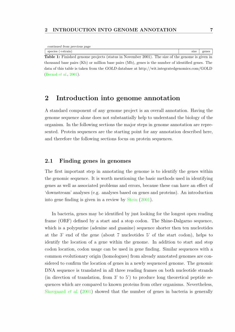
1 Finished genome projects . . . . . . . . . . . . . . . . . . . . . . . . . 7
2 PAM70 amino acid substitution matrix . . . . . . . . . . . . . . . . . 23
List of Figures
1 Metabolic pathways in the V. cholerae cell . . . . . . . . . . . . . . . 18
2 Distribution of random alignment scores . . . . . . . . . . . . . . . . 27
3 The PSI-BLAST procedure . . . . . . . . . . . . . . . . . . . . . . . 30
4 A two state hidden Markov model . . . . . . . . . . . . . . . . . . . . 36
5 An HMM for multiple sequence alignments . . . . . . . . . . . . . . . 38
6 Relationship between sequence identity and structural similarity . . . 39
7 Multi-functionality of homologous domains . . . . . . . . . . . . . . . 40
8 GSK3β protein surface and active site . . . . . . . . . . . . . . . . . 42
9 Superposition of ribonuclease H and integrase . . . . . . . . . . . . . 44
10 Superposition of lysozyme and α-lactalbumin . . . . . . . . . . . . . . 46
11 The SCOP classification . . . . . . . . . . . . . . . . . . . . . . . . . 50

Preface
The available sequence data from the finished genome projects provides biological
science with a huge and valuable source of data. The genetic information together
with its derived data such as protein sequences and structures, expression levels
and sub-cellular location has to be managed, understood and exploited for human
benefit. It is a long and challenging way from the raw sequence data (the genome)
to only a basic understanding of how an organism developed in evolution and how it
functions. It is not just the sum of the parts that makes life but a complex regulatory
network of interactions involving many components. The sequence data is further
analysed in large scale experiments such as expression profiles and protein interac-
tion networks which in turn increases the amount data to be analysed dramatically.
Bioinformatics organises and integrates all parts of the experimentally generated
data as well as connecting them to gain understanding of biological systems.
Bioinformatics is a relatively young discipline as a science with components from
software engineering. Bioinformatics aims to analyse and understand biological data,
but a hypothesis is not necessarily required when it comes to the description, man-
agement and interpretation of the experimentally generated data. Currently, the
development of new algorithms, recycling of algorithms from other areas such as
natural language processing, data management, the interpretation of data and their
relationships as well as supporting biologists working in a specific system is included
in bioinformatics.

1 GENOME SEQUENCING PROJECTS 5
1 Genome sequencing projects
As of November 2001 there were 67 completely sequenced bacterial and archaea
bacterial genomes and eleven eukaryotic genomes (for which at least one chromo-
some has been sequenced) available. The draft human genome sequence with >3,000
mega bases was published in February 2001. Table 1 gives an overview of the fin-
ished sequencing projects. In addition there are roughly 300 ongoing prokaryotic
and about 80 eukaryotic public and commercial sequencing projects (data from In-
tegrated Genomics Inc., http://wit.integratedgenomics.com/GOLD, Bernal et al.
(2001)). Many of the sequenced genomes are from pathogenic organisms such as
the recently published Yersinia pestis genome that causes plague (Heidelberg et al.,
2000) or the two Salmonella strains (Parkhill et al., 2001a; McClelland et al., 2001).
The genome sequence reveals many secrets about the organism that may help to
identify potential drug targets. The ideal target might be a key protein in an essen-
tial pathway specific to the pathogenic organism.
species (+strain) size genes
Archaea
Methanococcus jannaschii DSM 2661 (Bult et al., 1996) 1664 Kb 1750
Methanobacterium thermoautotrophicum delta H (Smith et al., 1997) 1751 Kb 1918
Archaeoglobus fulgidus DSM4304 (Klenk et al., 1997) 2178 Kb 2493
Pyrococcus horikoshii (shinkaj) OT3 (Kawarabayasi et al., 1998) 1738 Kb 1979
Aeropyrum pernix K1 (Kawarabayasi et al., 1999) 1669 Kb 2620
Pyrococcus abyssi GE5 (no reference) 1765 Kb 1765
Halobacterium sp. NRC-1 (Ng et al., 2000) 2014 Kb 2058
Thermoplasma acidophilum (Ruepp et al., 2000) 1564 Kb 1478
Thermoplasma volcanium GSS1 (Kawashima et al., 2000) 1584 Kb 1524
Sulfolobus solfataricus P2 (She et al., 2001) 2992 Kb 2977
Sulfolobus tokodaii 7 (Kawarabayasi et al., 2001) 2694 Kb 2826
Bacteria
Haemophilus influenzae KW20 (Fleischmann et al., 1995) 1830 Kb 1850
Mycoplasma genitalium G-37 (Fraser et al., 1995) 580 Kb 468
Synechocystis sp. PCC6803 (Kaneko et al., 1996) 3573 Kb 3168
Mycoplasma pneumoniae M129 (Himmelreich et al., 1996) 816 Kb 677
Escherichia coli K12- MG1655 (Blattner et al., 1997) 4639 Kb 4289
Helicobacter pylori 26695 (Tomb et al., 1997) 1667 Kb 1590
Bacillus subtilis 168 (Kunst et al., 1997) 4214 Kb 4099
Borrelia burgdorferi B31 (Fraser et al., 1997) 1230 Kb 1256
Aquifex aeolicus VF5 (Deckert et al., 1998) 1551 Kb 1544
Mycobacterium tuberculosis H37Rv (lab strain) (Cole et al., 1998) 4411 Kb 4402
Treponema pallidum subsp. pallidum Nichols (Fraser et al., 1998) 1138 Kb 1041
Chlamydia trachomatis serovar D (Stephens et al., 1998) 1042 Kb 896
Rickettsia prowazekii Madrid E (Andersson et al., 1998) 1111 Kb 834
Helicobacter pylori J99 (Alm et al., 1999) 1643 Kb 1495
Chlamydia pneumoniae CWL029 (Kalman et al., 1999) 1230 Kb 1052
continued on next page

1 GENOME SEQUENCING PROJECTS 6
continued from previous page
species (+strain) size genes
Thermotoga maritima MSB8 (Nelson et al., 1999) 1860 Kb 1877
Deinococcus radiodurans R1 (White et al., 1999) 3284 Kb 3187
Ureaplasma urealyticum serovar 3 (Glass et al., 2000) 751 Kb 650
Campylobacter jejuni NCTC 11168 (Parkhill et al., 2000b) 1641 Kb 1654
Chlamydia pneumoniae AR39 (Read et al., 2000) 1229 Kb 1052
Chlamydia trachomatis MoPn Nigg (Read et al., 2000) 1069 Kb 924
Neisseria meningitidis MC58 (serogroup B) (Tettelin et al., 2000) 2272 Kb 2158
Neisseria meningitidis Z2491 (serogroup A) (Parkhill et al., 2000a) 2184 Kb 2121
Bacillus halodurans C-125 (Takami & Horikoshi, 2000) 4202 Kb 4066
Chlamydia pneumoniae J138 (Shirai et al., 2000) 1228 Kb 1070
Xylella fastidiosa CVC 8.1.b clone 9.a.5.c (Simpson et al., 2000) 2679 Kb 2904
Vibrio cholerae serotype O1, Biotype El Tor, strain N16961 (Heidelberg et al., 2000) 4000 Kb 3885
Pseudomonas aeruginosa PAO1 (Stover et al., 2000) 6264 Kb 5570
Buchnera sp. APS (Shigenobu et al., 2000) 640 Kb 564
Mesorhizobium loti MAFF303099 (Kaneko et al., 2000) 7596 Kb 6752
Escherichia coli O157:H7 EDL933 (Perna et al., 2001) 4100 Kb 5283
Mycobacterium leprae TN (Cole et al., 2001) 3268 Kb 1604
Escherichia coli O157:H7. Sakai (Hayashi et al., 2001) 5594 Kb 5448
Pasteurella multocida Pm70 (May et al., 2001) 2250 Kb 2014
Caulobacter crescentus (Nierman et al., 2001) 4016 Kb 3737
Streptococcus pyogenes SF370 (M1) (Ferretti et al., 2001) 1852 Kb 1696
Lactococcus lactis IL1403 (Bolotin et al., 2001) 2365 Kb 2266
Staphylococcus aureus N315 (Kuroda et al., 2001) 2813 Kb 2594
Staphylococcus aureus Mu50 (Kuroda et al., 2001) 2878 Kb 2697
Mycobacterium tuberculosis CDC 1551 (no reference) 4403 Kb 4187
Mycoplasma pulmonis (Chambaud et al., 2001) 963 Kb 782
Streptococcus pneumoniae TIGR4 (Tettelin et al., 2001) 2160 Kb 2094
Clostridium acetobutylicum ATCC 824D (Nolling et al., 2001) 4100 Kb 4927
Sinorhizobium meliloti 1021 (Galibert et al., 2001) 6690 Kb 6205
Streptococcus pneumoniae R6 (Hoskins et al., 2001) 2038 Kb 2043
Agrobacterium tumefaciens C58 (Wood et al., 2001) 4915 Kb 4554
Rickettsia conorii Malish 7 (Ogata et al., 2001) 1268 Kb 1374
Yersinia pestis CO-92 Biovar Orientalis (Parkhill et al., 2001b) 4653 Kb 4012
Salmonella typhi CT18 (Kuroda et al., 2001) 4809 Kb 4600
Salmonella typhimurium,LT2 SGSC1412 (McClelland et al., 2001) 4857 Kb 4597
Listeria innocua Clip11262, rhamnose-negative (Glaser et al., 2001) 3011 Kb 2981
Listeria monocytogenes EGD-e (Glaser et al., 2001) 2944 Kb 2855
Eukaryota
Saccharomyces cerevisiae S288C (No authors listed, 1997) 12069 Kb 6294
Caenorhabditis elegans (The C. elegans Sequencing Consortium, 1998) 97000 Kb 19099
Drosophila melanogaster (Adams et al., 2000) 137000 Kb 14100
Arabidopsis thaliana (The Arabidopsis Genome Initiative, 2000) 115428 Kb 25498
Guillardia theta (Douglas et al., 2001) 551 Kb 464
Leishmania major Friedlin Chromosome 1 (Myler et al., 1999) 257 Kb 79
Plasmodium falciparum 3D7 Chromosome 2 (Gardner et al., 1998) 947 Kb 205
Plasmodium falciparum 3D7 Chromosome 3 (Bowman et al., 1999) 1060 Kb 220
Homo sapiens (Lander et al. (2001) and Venter et al. (2001)) >3000 Mb 35000
continued on next page
2 INTRODUCTION INTO GENOME ANNOTATION 7
continued from previous page
species (+strain) size genes
Table 1: Finished genome projects (status in November 2001). The size of the genome is given inthousand base pairs (Kb) or million base pairs (Mb), genes is the number of identified genes. Thedata of this table is taken from the GOLD database at http://wit.integratedgenomics.com/GOLD(Bernal et al., 2001).
2 Introduction into genome annotation
A standard component of any genome project is an overall annotation. Having the
genome sequence alone does not substantially help to understand the biology of the
organism. In the following sections the major steps in genome annotation are repre-
sented. Protein sequences are the starting point for any annotation described here,
and therefore the following sections focus on protein sequences.
2.1 Finding genes in genomes
The first important step in annotating the genome is to identify the genes within
the genomic sequence. It is worth mentioning the basic methods used in identifying
genes as well as associated problems and errors, because these can have an effect of
‘downstream’ analyses (e.g. analyses based on genes and proteins). An introduction
into gene finding is given in a review by Stein (2001).
In bacteria, genes may be identified by just looking for the longest open reading
frame (ORF) defined by a start and a stop codon. The Shine-Dalgarno sequence,
which is a polypurine (adenine and guanine) sequence shorter then ten nucleotides
at the 3’ end of the gene (about 7 nucleotides 5’ of the start codon), helps to
identify the location of a gene within the genome. In addition to start and stop
codon location, codon usage can be used in gene finding. Similar sequences with a
common evolutionary origin (homologues) from already annotated genomes are con-
sidered to confirm the location of genes in a newly sequenced genome. The genomic
DNA sequence is translated in all three reading frames on both nucleotide strands
(in direction of translation, from 3’ to 5’) to produce long theoretical peptide se-
quences which are compared to known proteins from other organisms. Nevertheless,
Skovgaard et al. (2001) showed that the number of genes in bacteria is generally

2 INTRODUCTION INTO GENOME ANNOTATION 8
overpredicted (in A. pernix they estimated 100% gene overprediction which is by far
the most extreme in their analysis).
Gene identification in eukaryotic genomes is far more problematic than in prokary-
otic genomes. This is due to the exon-intron structure of genes and the lack of
obvious sequence features such as a Shine-Dalgarno sequence to distinguish between
coding and non-coding regions . Despite the start codon there is no clear landmark
where a gene starts on a eukaryotic chromosome. Rule based ab initio gene iden-
tification methods such as GeneScan (Burge & Karlin, 1997) or Grail (Uberbacher
& Mural, 1991; Roberts, 1991; Xu et al., 1994) that employ statistical methods (for
example hidden Markov models, see section 3.7), have been shown to identify only
40% of the existing genes with their exon-intron structure. About 70% of these
predictions are to some extent wrong, i.e. do not corresponds to the correct gene
structure (Reese et al., 2000). On the other hand 90% of the predictions include at
least a fraction of the real gene. The use of experimental data as described above
for bacterial gene identification improve eukaryotic gene finding. For example, the
human genome sequence as defined by the ENSEMBL project version 1.2 (Hubbard
et al. (2002), http://www.ensembl.org), contains more than 150,000 predicted genes,
but only about 25,000 genes are either confirmed by expressed sequenced tags (ESTs
derived from mRNA of expressed genes) or homologues in a different organism. Be-
cause of the extensive exon-intron structure and the small fraction of actual coding
sequences in the human genome (estimated at about 1.5% of the genome, Lander
et al. (2001)), two predicted genes may in fact be one larger gene, or a larger gene
may be in fact several genes. A positive view on the human genome shows that
25,000 of at least 30,000 genes have been identified with the help of experimental
data (ESTs and homologues), which corresponds to nearly 85% of the estimated
number of genes in the genome.
The expected number of genes in the human genome is between 30,000 and
40,000 (Lander et al., 2001), thus there are theoretically still 5,000 to 15,000 genes
missing. The genome sequences of other higher eukaryotes, in particular those of
mouse (M. musculus), rat (R. norvegicus) and the puffer fish (Fugu rubripes) will
help to identify genes within these genomes and that of human, because of the higher
sequence conservation within exons compared to non coding regions. The mouse and
rat genome projects were established mainly because these organisms are used as
models in biology. The genome sequence (with the confirmed set of genes) will
2 INTRODUCTION INTO GENOME ANNOTATION 9
accelerate the progress with which molecular biologists clone and analyse specific
parts of the genome. The puffer fish project was deliberately established to enhance
gene finding and interpretation of the human genome sequence. A draft sequence
of the puffer fish project has been available since October 2001. The extent of the
coding sequences is estimated to be similar to that of human, but the overall size of
the genome (350 to 400 mega bases) is just about one eighth of the human genome
(>3,000 mega bases). The sequence conservation between the dense coding regions
of the puffer fish and the corresponding regions in the human genome is expected
to reveal currently unidentified genes.
In interpreting results from the analysis of the identified peptide sequence reper-
toire of a genome one has to keep in mind that the absence of a particular protein
does not necessarily mean that the genome contains no coding sequence for this
peptide, it may just have been missed in the interpretation of the genome.
2.2 Functional classification of genes and proteins
Once the genes are identified within a genome, they have to be functionally charac-
terised. Usually the genes are compared to a set of already functionally characterised
genes. Since a protein sequence is more conserved in its amino acid sequence than
the corresponding nucleotide sequence of the gene (because of the redundant genetic
code), sequence comparisons for functional annotation are performed at the peptide
level.
Function, at the level of a functional classification of proteins, is the description
of the biochemical function or a combination of several biochemical functions. A
functional annotation is generally derived from one or more homologous sequences
for which a functional description has been generated previously. However, only for
a fraction of annotated proteins has the biochemical activity been proven experi-
mentally (Ursing et al., 2002). Section 4.1 discusses the quality and the limitations
of functional transfer between homologues.
The majority of proteins in a genome consist of more than one protein domain.
A domain can be considered as the smallest functional and evolutionary unit of pro-
teins and is generally found in different proteins in combination with other domains
2 INTRODUCTION INTO GENOME ANNOTATION 10
of the same (repeats) or of different type (Apic et al., 2001; Qian et al., 2001). The
potential multi-domain character of proteins may need a list of biochemical func-
tions, which depends on the level detail of the annotation. For example a protein
with a NAD(P) binding domain and a dehydrogenase domain may just be described
as a dehydrogenase or in more detail as a protein that binds NAD(P) and has a
dehydrogenase activity (the NAD(P) binding domain may be a ‘helper’ domain to
fulfil the proteins biochemical function). In most cases the functional annotation
does not include the biological function, e.g. a human protease may be found in
a different biological context such as digestion, during development or in wound
healing. The main concepts in functional protein annotation are:
• Finding a homologous sequence that has been functionally characterised pre-
viously, the main databases containing such protein sequences are SwissProt
and PIR.
• Identifying domains within a protein sequence via homology. The main do-
main databases with functional descriptions are PFAM, SMART, ProDom and
InterPro. (Structural domain databases are discussed later.)
• Finding conserved patterns or motifs (these motifs are generally shorter than a
domain and may not include an independent folding unit). The main databases
maintaining collections of patterns or motifs associated with a function are
Prosite, Prints and Blocks.
2.3 Major resources used in protein annotation
The following sections give a more detailed view of the contents of some of the
available databases, including an overview of how these databases are constructed.
The first issue each year of the journal Nucleic Acids Research (in particular those
from 1999 on) contains articles about biological databases. The first 2002 issue
describes 112 different specialised biological databases.
2.3.1 The main source database GenBank and EMBL
All the specialised databases described below are based on the basic sequence databa-
ses. The major nucleotide sequence databases are GenBank (Benson et al., 2002) and
EMBL (Stoesser et al., 2002). Usually nucleotide sequences (or a nucleotide sequence
together with its peptide sequence) are submitted to either of these databases. Also,

2 INTRODUCTION INTO GENOME ANNOTATION 11
GenBank and EMBL update each other, so that both databases, with some de-
lay, contain the same sequences. If possible the submitted nucleotide sequences are
translated into a theoretical peptide sequence. These peptide sequences generate the
TrEMBL database (translated EMBL) and the GenPept database (translations from
GenBank). In addition, all publicly available genome sequences are submitted to
one of these databases. GenBank and EMBL entries contain information associated
with the sequence: literature references, authors, gene or protein names, taxonomic
information of the source organism and a feature table that lists all known features
(e.g. a ribosomal binding site for a bacterial ORF or an exon for a eukaryotic se-
quence) with their location in the sequence. GenPept and TrEMBL contain more
than 800,000 non-redundant peptide sequences (status 11/2001). EMBL/TrEMBL
is available from the EBI (http://www.ebi.ac.uk) and GenBank/GenPept is avail-
able from the NCBI (http://www.ncbi.nlm.nih.gov).
2.3.2 The SwissProt protein database
The SwissProt database (Bairoch & Apweiler, 2000) historically collected sequences
from protein sequencing experiments, i.e. the sequence information was directly
taken from the peptide sequence and not by translating a coding region of a gene.
SwissProt (version 40.11) contains 105,322 protein sequences. TrEMBL sequences
are transfered to SwissProt if there is sufficient evidence for the existence of the
gene product. The procedure for integrating new entries into SwissProt includes re-
viewing by human experts (database curators) and external consultants with expert
knowledge about a particular protein family. A SwissProt entry contains, in addi-
tion to the peptide sequence and literature references, comments about the functions
associated with the protein (edited by the human experts), keywords that describe
the function and a structured feature table that describes regions or positions in the
sequence such as post-translational modifications, domains and sites (e.g. an ATP
binding site).
2.3.3 The PIR protein database
The Protein Information Resource (PIR, Barker et al. (2000)), contains about
200,000 protein sequences (status in 2001). Like SwissProt, the database aims to
provide high quality annotation. Automatically generated annotations are reviewed
and edited by PIR staff, and consultant scientists who review specific parts of the

2 INTRODUCTION INTO GENOME ANNOTATION 12
database. Sequence entries are classified according to their status to which there is
evidence of their existence, e.g. for entries that are classified as experimental there is
some experimental evidence, and predicted proteins from theoretical coding regions
are classified as predicted. Also the annotation is classified into validated or similarity
according to the available evidence. PIR further clusters sequences in families and
superfamilies based on sequence similarity. Because PIR and SwissProt both get
their sequences from translated coding regions of the major nucleotide databases,
there is redundancy between the two databases.
2.3.4 The PFAM, SMART and ProDdom domain and family databases
The domain and protein family databases described here are generated by splitting
protein sequences into domains and then clustering similar domains into a family.
Annotating proteins according to their domain composition generally leads to more
detail than annotating the protein as a single unit.
PFAM is a database of protein domain families (Bateman et al., 2002), based on
protein sequences from SwissProt and TrEMBL. It contains a set of curated mul-
tiple sequence alignments, each representing a protein family. From these multiple
alignments hidden Markov models (see section 3.7) are built, which are in turn used
to search the protein sequence databases to find new members and to expand a
family. The final database PFAM-A provides a high quality description of the fam-
ilies which can help in annotating newly sequenced genomes. Most of the PFAM-A
families also contain a functional text description, cellular location of the members
of the family, relevant literature references and links to taxonomic groups in which
a family is found. PFAM-A is manually curated. Another part of PFAM (PFAM-
B) contains potential domain families for which there is not enough evidence to be
placed into PFAM-A. PFAM-B entries are mainly taken from families of the large
ProDom database (see below). PFAM-B contains more members and families than
PFAM-A but is of lower quality. PFAM-B and ProDom are used to update and
curate PFAM-A. PFAM-A version 6.6 (August 2001) contains 3071 families. PFAM
is available at The Sanger Centre (http://www.sanger.ac.uk/Software/Pfam).
SMART (a Simple Modular Architecture Research Tool, Letunic et al. (2002)),
like PFAM, is a domain database but originally focused on domains in eukaryotic
signal transduction. Recent SMART versions (November 2001) also include a wide

2 INTRODUCTION INTO GENOME ANNOTATION 13
range of other domain types (more than 600 domain families). Domain families are
constructed in a similar way to PFAM, but the initial step to create a seed multiple
sequence alignment involve manual editing and, if available, consideration of pro-
tein structure, or homologues of proteins of known structure. Hidden Markov models
are constructed from these alignments that are used to search the protein sequence
database to collect new family members. The hidden Markov models are then re-
built, and the search starts again until no more members are found. In addition each
member of a family is compared to the sequence database using the homology search
method PSI-BLAST (see section 3.5) to collect new family members. Alignments
are updated, e.g. when the three dimensional structure of a member is published,
to re-assess domain boundaries of the family. SMART is based on sequences from
SwisProt and TrEMBL. The database is available at the EMBL (http://smart.embl-
-heidelberg.de). The web-interface also allows the user to search for proteins of a
given domain architecture (domain combinations).
ProDom (Corpet et al., 2000) is a domain database with a larger sequence cover-
age than PFAM or SMART. Over 75% of the proteins from SwissProt and TrEMBL
can be assigned to ProDom families (status 2001). There are about 44,000 ProDom
domain families with more than one member. From version 35 onwards, the ProDom
database includes manual inspection of protein families by scientific consultants.
PFAM-A (see above) is used to increase the quality of ProDom. Domain families
are generated via PSI-BLAST homology searches (Sonnhammer & Kahn, 1994).
Two proteins may share only one homologous region in their sequence, which can
be a single domain or several domains. These regions are then used as queries in
subsequent PSI-BLAST searches to find additional significant alignments. This pro-
cedure is repeated until the regions cannot be split or truncated anymore because
no further homologous regions are found. The identified regions are then consid-
ered to be domains, and all homologous regions belong to one family. As a quality
control, recent versions of ProDom assign consistency indicators to each family (for
example sequence variation within a family). ProDom-GC is a ProDom version that
clusters protein sequences from complete genomes into families. Both databases are
available at http://prodes.toulouse.inra.fr/prodom/doc/prodom.html.
2 INTRODUCTION INTO GENOME ANNOTATION 14
2.3.5 Motif databases: PROSITE, PRINTS and BLOCKS
The PROSITE database (Falquet et al., 2002) is a collection of pattern descriptions
that usually are associated with a biochemical function. These signatures are gen-
erated from curated multiple sequence alignments and generally describe conserved
positions within a domain family. Signatures are represented as regular expression
patterns. Since patterns are not flexible (i.e. a pattern matches a sequence region
or it does not), the extent to which patterns identify a particular motif is limited.
To overcome this limitation, signature profiles have been developed which assign a
score to each of the 20 amino acids at each position of the signature according to
the frequency of which each amino acid is found at a particular position. Further,
alternative protein structure-based profiles and methods involving hidden Markov
models have been employed. A PROSITE entry can be associated with a functional
description and reasons that lead the construction of a pattern or profile. PROSITE
version 16.50 (November 2001) contains 1103 documents describing 1493 patterns
and profiles, and is available at http://www.expasy.org/prosite.html, it is updated
in parallel with SwissProt.
PRINTS (Attwood et al., 2002) and PRINTS-S (a recent development of the
original PRINTS) is a collection of protein fingerprints. The concept behind finger-
prints is that a protein can be represented by several conserved motifs. A fingerprint
is an ordered list of these motifs that describes a protein family. PRINTS-S is a
database for protein sequences rather than domains, although its components (the
single motifs) may be characteristic for a particular type of domain. The procedure
to build the fingerprints starts with manual curated multiple sequence alignments,
and then a series of conserved regions are extracted to construct motifs. This pro-
cedure includes manual intervention. The sequence database is searched iteratively
with these motifs to expand and gain confidence of the motifs. PRINTS-S contains
its own search software FingerPRINScan. The database is built from SwissProt
and TrEMBL. Each entry is associated with bibliographic information, functional
descriptions, lists of matching sequences and comments. The database (PRINTS-
S version 10, based on PRINTS version 32, November 2001) contains about 9,800
individual motifs and about 1,600 fingerprints. It is available at http://www.bioinf.-
man.ac.uk/dbbrowser/PRINTS.
The BLOCKS database (Henikoff et al., 1999, 2000) is similar to PRINTS. It

2 INTRODUCTION INTO GENOME ANNOTATION 15
contains a list of motifs that are representative for a family. Motifs in the BLOCKS
database are called blocks. To generate these blocks, protein family databases such
as PFAM-A, PRINTS, ProDom and Domo (Gracy & Argos, 1998) are used. Se-
quences for each family of these databases are re-aligned via a non-gapped multiple
local alignment procedure and converted into non-overlapping blocks. Thus, the
BLOCKS database identifies local motifs within given protein families but does not
find new protein families (because it uses domain families of the existing domains
databases as input). The BLOCKS database can be searched with sequences via
the BLIMPS (Henikoff et al., 1995) program that identifies individual blocks and
then combines hits belonging to the same family. Sequences can also be searched
against the database via the IMPALA program (see section 3.6). BLOCKS (June
1999) contains about 9,500 individual blocks and more than 2,000 families. It is
available at http://www.blocks.fhcrc.org.
2.3.6 InterPro: A combination of databases
InterPro (Apweiler et al., 2001), a recent database development from the EBI
(http://www.ebi.ac.uk/interpro), integrates most of the above databases. InterPro
itself does not contribute any new information, and its power comes from having
all the above databases in one place providing a range of evidence for a protein to
belong to a certain InterPro entry. InterPro is divided into families (3,532 entries),
domains (1,068 entries), repeats (74 entries) and post-translational modifications
(15 entries). A short description and an abstract about the biochemical function,
the biological role and matches against the SwissProt and TrEMBL databases are
included for each entry. InterPro also contains, like recent PFAM versions, families
for which the function is unknown, but where there is evidence for the conservation
of this family, domain or motif.
A family can be described by a set of characteristics from the above databases,
e.g. the thiolase family (InterPro entry IPR002155) is described by two PFAM en-
tries and three Prosite patterns. Sequences can be searched against InterPro via the
InterProScan software package (Zdobnov & Apweiler, 2001).
InterPro is a ‘modern’ database. It is distributed in XML format and is, together
with the integrated search engine InterProScan, a step towards solving common
bioinformatics problems such as standardisation, automatisation and distribution.

2 INTRODUCTION INTO GENOME ANNOTATION 16
A list of InterPro families is now commonly reported as an initial analysis of a newly
sequenced genome (e.g. Lander et al. (2001); Rubin et al. (2000) and http://www.-
ebi.ac.uk/proteome).
2.4 Gene Ontology (GO), a controlled vocabulary for ge-
nome annotation
A recent commentary published in the journal Nature (Pearson, 2001) summarises
problems and inconsistencies in gene (and protein) nomenclature and stresses the
importance of an ontology for gene names and functions to overcome problems in
annotation. In GO, descriptive terms and phrases are used to annotate a gene rather
than using gene and protein names such PMS1 or TFIIA. These terms are organised
in a hierarchy (a tree of terms and phrases) with the more general terms such as
transcription or fatty acid metabolism as the root for more detailed terms or phrases
such as RNA polymerase II transcription factor or fatty acid hydrolase. The set
of terms and phrases is stored in a central GO database maintained at Stanford
University. However, different GOs may be constructed for special purposes. New
terms can be inserted into the GO-tree. GO is also able to cope with synonyms
and can describe biological function. Using a system with a controlled vocabulary
organised in a tree as in GO allows automatic comparison of annotations between
genomes at different levels of the tree (i.e. at different level of detail, for example
to test for the existence of enzymatic pathways between genomes). The central GO
resource is located at http://www.geneontology.org, see also Lewis et al. (2000);
Ashburner et al. (2000); The Gene Ontology Consortium (2001).
2.5 Putting everything together to find pathways
At a higher level, genome annotation aims to identify complete biological subsys-
tems such as metabolic pathways or signalling pathways. The usual approach is
to compare all members of a pathway (e.g. for glycolysis) in a model organism
to the proteins of a newly sequenced genome. The comparison is carried out via
the standard homology search methods (see section 3 below). This approach gen-
erally identifies the fundamental pathways such as glycolysis in a newly sequenced
genome. If members of a pathway cannot be identified, this does not necessarily
mean the pathway is incomplete. The homology based comparison may just have
missed some members of that pathway because of insufficient similarity (although
3 HOMOLOGY BASED SEQUENCE COMPARISON METHODS 17
the homologues are present), or there may be alternative routes bypassing the known
proteins of that pathway. There are three major database systems available that
implement the above approach for metabolic pathways: The partly freely available
WIT system from Integrated Genomics (this system is now known as ERGO and is
no longer freely available for academic use, http://www.integratedgenomics.com/),
the KEGG (Kanehisa et al., 2002) database (Kyoto Encyclopedia of Genes and
Genomes) freely available for academic use and EcoCyc (Karp et al., 2002), a sys-
tem that describes metabolic pathways in E. coli (this database recently has been
made freely available for academic users).
The publication of the genome sequence of the cholera bacterium V. cholerae
(Heidelberg et al., 2000) contains an overview of some of the identified pathways in
this bacterium and can serve as an example of how to represent complex pathways
information in a comprehensive way (see figure 1).
3 Homology based sequence comparison methods
If two genes or proteins have diverged from a common ancestor they are by definition
homologues. Further, homologues within the same species are paralogues, and often
have different functions due to specialisation. The closest homologues with generally
the same biochemical function in two species are orthologues (Tatusov et al., 1997,
2001). Whether two sequences are homologues can be measured by their sequence
similarity for which there are different definitions and methods.
As mentioned in the introductory sections above, identifying homologous se-
quences is often the first step in annotating a newly sequenced gene. The homo-
logue may already have some functional annotation that may then be transfered to
the newly sequenced gene (or protein). Section 4.1 explains the conditions under
which this transfer is considered to be reliable. The sections below explain the most
common sequence search methods and their definition of similarity.

3 HOMOLOGY BASED SEQUENCE COMPARISON METHODS 18
Origin and function of the small chromosome of V. choleraeSeveral lines of evidence suggest that chromosome 2 was originally amegaplasmid captured by an ancestral Vibrio species. The phyloge-netic analysis of the ParA homologues located near the putativeorigin of replication of each chromosome shows chromosome 1ParA tending to group with other chromosomal ParAs, and theParA from chromosome 2 tending to group with plasmid, phageand megaplasmid ParAs (see Supplementary Information). Ingeneral, genes on chromosome 2, with an apparently identicalfunctioning copy on chromosome 1, appear less similar to ortho-logues present in other g-Proteobacteria species (see Supplemen-tary Information). Also, chromosome 1 contains all the ribosomalRNA operons and at least one copy of all the transfer RNAs (fourtRNAs are found on chromosome 2, but there are duplicates onchromosome 1). In addition, chromosome 2 carries the integronregion, an element often found on plasmids26. Finally, the bias in thefunctional gene content is more easily explained, if chromosome 2
was originally a megaplasmid (Fig. 4). The megaplasmid presum-ably acquired genes from diverse bacterial species before its captureby the ancestralVibrio. The relocation of several essential genes fromchromosome 1 to the megaplasmid completed the stable capture ofthis smaller replicon. Apparently this capture of the megaplasmidoccurred long enough ago that the trinucleotide composition andpercentage G+C content between the two chromosomes hasbecome similar (except for laterally moving elements such as theintegron island, bacteriophage genomes, transposons, and so on).The two chromosome structure is found in other Vibrio species19
suggesting that the gene content of the megaplasmid continues toprovide Vibrio with an evolutionary advantage, perhaps within theaquatic ecosystem where Vibrio species are frequently the dominantmicroorganisms14,16.It is unclear why chromosome 2 has not been integrated into
chromosome 1. Perhaps chromosome 2 plays an important special-ized function that provides the evolutionary selective pressure to
articles
NATURE |VOL 406 | 3 AUGUST 2000 |www.nature.com 479
���
�����
����� �����
���� �� ��� � ������������������ ��� � ��� � �
��� � � ��
��� ��� ��� �� � �
� �����!� � � ��
"�� ��#���$�� �� �� �� ��������� ��� � �����
�������� ���
% ��&��� ��
&��� �� ��#�!� ���� � � ���!� '
$!� ����#���� �
(�� )*(�+���*,-�!�.�
)/(�+.��021��
34567 458 98
: ;<=>?@>: @?@A BA
CED FEDGCEHIEJLKGIEJ�HGJ�M MN O FEPEQO R
D JSD�TJVUGW I O F W X�CN CED F JLYECN PGJSYEN P�O FECN O FEP Q�O R
ZE[ \ \ ]�^�_V` a�b` cVd ]Ve \ fEg d�` d[GeEa�h�gEiSj [EaV[ \ ` cLe
(�� (��*�����.�.�
� k�! ����(���� .����� �
% ��� &��� �lm�n o���0/n
�!p!0q(�r s-�
�� !� � �
0-p�s�r �.m�r s-��-p.)/r s�r s-�
��1.�.�/p.���!�.�
�
(�������0t1��
)*(Eu���0-)*�.s
v � � v � �� ���
(�� �-(���s�r s��1���p�r s��(�� �.p�u�����0*�-m��ts
"�� w� � �!� � �������� �� ��
�����x�.�����
��1.����p��*)/r s��
�!�!� ��y-�ot���
���!���� � k���� m!o
z�{�|�}�~ � ���
� � ���� � �
���
���
���
�t�������/�-�S�/�
��� ���
��� ���
` j cLe�� � � � �� �G� � � � ` �Vj ` cS�G[E_ \ ` e� � �L��� E� ¡L� ¢£ ` eG_¤ ¥L¦ § � �L� f gG¨�` e© ¦Gª �� G� ¡
��� ��� �«�¬ L®#�! � k�� �¯��� �!� � % �&°� � �
s�,2s�l ±.² «�³
´�µV¶¦E· � § � �L� G� ¸fEgE¨!g¹ ¹ º § � �L� G� ¡
aSj »EiVd� ¼ ½V� µ �\ cG¾V` eEd� ½G� � �¿ ` ÀGcL¿ ]EdE[E_E_VfE[Gj ` aVg ÁÂ�à [Ge \ ` iVgGeG�VÄ � ÅVÆL� Ç
È2É.Ê Ë Ì Í Ì Î*Ï Ì Ð�ÌÑ Ì Ò Ì Ó Ì Ô
Õ ÈtÖ�×ÙØ Ú!Û!Ü Ú.Ý Þ
ß!à ÝâáGã ä�å�Ê.ã ã ä.æ�ä.ç.èéÙê.ë ê æ�å�Ê.ç.Ê�×
��k !&t��� ���� � ���� $� ��� �
lV±.ì�í î
�/ï
ðLñSðSò�óLô�Â�õÙóLôL^�õ�ö�¶SÂ�ô�ó�ò�÷L^�� õm!o m�o m!o
��ø���'�� ��� ù���#���� �� ú�û�í ü�ý þ�ý ÿ��!ú�û «�® ý � ý ³
ù� � ������� �l�����²�î% ��� &��� �� �l �
s!�� ¯ '�� ���� ù���#���� �� �� �l �
s!�� ¯ ��� � � �� �l�û�� í ���#��� �� �¯ % ��� &���
$��� ���� ���!� '� ����� ® ý ��ý ³
&��� � ��� � � î�ý ��ý���ý��
� � ù����� ¬ ��� ® ý ��ý ³ ý �
(�� � ��� �� �$�� ������ ���
����� v k��� �l�û"!#�#$v k���� v k��� !l�²±�í ®
����� v k��� �� "�l " �
����� v k��� û%!�� ® ý ü�ý�&�ý�'
v k���� v k��� (� �l �±���í ® ý ��ý ³ ý �&���� ��ù�'! � ���&� ì�ú ® ý ��ý ³
��k���ø % �&q� � � v � ��� ��
����$��� % �& � � �
^�_Ej bLÁ hLÁ Z) [G¨�` ¿ ].� �G� ¼ �_E[ \ ` cLeEdð�¼ à ðV�) [G¨�` ¿ ]!� µE�
� ` �Vj ` cS�G[ _ \ ` ej gE_EgGÀ \ cSj* + ¦ §
v ��� ������ ��&,#��- �.� "/��
s!�� ¯ m0� � ø�l " �
,2$ n � l ��� í � � "�l �s!m21 ��v ��� ������ �!&�l!í ¬ , ® ý 3
� ��� ����� !l�í ! ¬ ü� � � v � � v k�! �l � í ¬
�2��� � % �& � � �4������ % �& � � �
�&°� ������� '���� 5�l �
v v � � '� ��� 5�l �
� v !� &°� '�� �¯v �� � ����� � ±�ì�í ® ý ��ý ³ ý �
�!� � $�� v v � � '� �ì±�± ® ý ��ý ³ ý ��ý �
�� $�� �� ¬ í 6 ý ÿ�ý ü�ýGþ
� !� � �l ��ú !³ � "#�
ù����l/� ¬ ²!þ
� � �� �� r r � l�- ��ì ® ý �
v ��� ������ �!&�l�, « ±
ó cSeVb*d ]Gd \ gG¨j gE_EgGÀE\ cSj � ¼ � � �
7 8 9 : ; < = < > 7 8 9 ? ; < = < >
@ ABCD E FEG
v ��� � �
s�� v �H��& � � �� "�l �
ZVñ ^�´�ðLñVñJI#K
õ�[EaVò) [G¨�` ¿ ]
�� $�� .� �¯��� �� � k�� v �� � ����� � �¯��� �� � k��
���'���� �� � � �¯� ����� � #
v � ��� �� �¯ v v � � '! % �& � � �
s!�� ¯ �� � �� � �� 5��v � ��� �� �¯ $�� ��� �&â�� �l ��� í ü� �l �
s!�� ¯ $�� �� �&��� !l ��� í �s!�� ¯ v � ��� � � �l ± « í ü
L M%N N OPMRQ"S TRURV/W X"Y�Z/[ \"V ] ^
_"`VN
a��cb
z�{�d�~ e�zRf�g
h ~ fji�}�k e�z/f�g
d�fjk k ejl�� e�z/fjmn ~ {�d h e�z/f
|jk {�d/e�z/foâ}jp�p�� h e�k
&��� � � v ��� � ì � ±j�
��+��.p���1.��r s-�
y�� �� ! �� (�� �� ! �� � ����!� ���� � �
)/(�+.��� ,/r s/�
+ Ä ·E§fEgG¨�g© ¦Gª §qRr sº�tV¹ u
)*� ����#��� �� ù�� v ���
,��/(�.�!�
)��-(��*����0-1��)*(Gu����!p�0*(2v v
,��-s�s�r ��0*(,��-s�s.0�1��
y�� (��*�����.�.�
H�p�+�����0t1��1�+���p.021��
�!p��.m��t(�0-1��s.� �*������u�(�)*(�+���021��/,*r s��
��m�r ��r s1����/p.��m
&t �� � ��
(�� v k� ! ��� �� � �� (���� � � v � � v k�� � ��� ����� �
)/(�+���0�s��/���
��p������k���� � ��&���
p�r 4.021��
\ fV` [G¨�` eEg%s_EcL¿ ` _V` eEdª wyx § � �S� zL� {
iL¿ ]G_·Jx �%| ´�µV¶·yx �/}
b¼ �ys� \ »Vb�Á ò�Á h K�dG�E^/s
�/�±
~ S U%N S T/S �"�����R�#� M"T�MJN S �/�� MJN �%�0M%Om�r 1���r y�r s-�
�"� �"�����y�%� �� �P� � �J�J�R� ���%� �R�J�R�J�%�%� �
� �#� �(� �P� �y���J� ��� �y� � � �%� �
�J� �R� ��� � � �%� �
% ��&��� �� ,��!��m.r 0�s�r s��
(�� � ����� � ����!� v � � v � �� ��� 0�� �������� ���� �k���&���� �� � �
$!� ����� ��0 n1��!p�r s-�
�!m�p���0�s.r s-�
(���������� �� �
(�� ��1��V�âp.���.�.�
'�� �& � �� v � &t �� � �t��� '
(�� � ����� ���'���� �� � �
Figure 3 Overview of metabolism and transport in V. cholerae. Pathways for energy
production and the metabolism of organic compounds, acids and aldehydes are shown.
Transporters are grouped by substrate speci®city: cations (green), anions (red),
carbohydrates (yellow), nucleosides, purines and pyrimidines (purple), amino acids/
peptides/amines (dark blue) and other (light blue). Question marks associated with
transporters indicate a putative gene, uncertainty in substrate speci®city, or direction of
transport. Permeases are represented as ovals; ABC transporters are shown as composite
®gures of ovals, diamonds and circles; porins are represented as three ovals; the large-
conductance mechanosensitive channel is shown as a gated cylinder; other cylinders
represent outer membrane transporters or receptors; and all other transporters are drawn
as rectangles. Export or import of solutes is designated by the direction of the arrow
through the transporter. If a precise substrate could not be determined for a transporter,
no gene name was assigned and a more general common name re¯ecting the type of
substrate being transported was used. Gene location on the two chromosomes, for both
transporters and metabolic steps, is indicated by arrow colour: all genes located on the
large chromosome (black); all genes located on the small chromosome (blue); all genes
needed for the complete pathway on one chromosome, but a duplicate copy of one or
more genes on the other chromosome (purple); required genes on both chromosomes
(red); complete pathway on both chromosomes (green). (Complete pathways, except for
glycerol, are found on the large chromosome.) Gene numbers on the two chromosomes
are in parentheses and follow the colour scheme for gene location. Substrates underlined
and capitalized can be used as energy sources. PRPP, phosphoribosyl-pyrophosphate;
PEP, phosphoenolpyruvate; PTS, phosphoenolpyruvate-dependant phosphotransferase
system; ATP, adenosine triphosphate; ADP, adenosine diphosphate; MCP, methyl-
accepting chaemotaxis protein; NAG, N-acetylglucosamine; G3P, glycerol-3-phosphate;
glyc, glycerol; NMN, nicotinamide mononucleotide. Asterisk, because V. cholerae does
not use cellobiose, we expect this PTS system to be involved in chitobiose transport.
© 2000 Macmillan Magazines Ltd
Figure 1: Schematic representation of the V. cholerae cell with a selection of metabolic pathwaysand transporters identified in the genome. This figure is an example how the huge amount ofinformation from genome annotation can be represented in a comprehensive and user friendly way.The figure is from Heidelberg et al. (2000).
.
3.1 Dynamic programming
The oldest sequence comparison method that is still part of recent methods was
developed by Needleman & Wunsch (1970). Their method is based on the general
dynamic programming algorithm which was introduced in the 1950s by Bellman
(1957), and allows the optimal alignment of two sequences. Two sequences with
length n and m form an n×m matrix. For each position in the matrix (n[i],m[j])
a numeric value scores how favourable a replacement of the residue/nucleotide n[i]
with m[i] or alternatively a deletion or insertion is. See section 3.2 below for a
discussion of substitution scores. Generally these are negative for unfavourable sub-
stitutions (e.g. aligning tryptophan with a lysine), and positive for conservative
substitutions such as lysine to arginine.
3 HOMOLOGY BASED SEQUENCE COMPARISON METHODS 19
Global sequence comparison via dynamic programming aligns two sequences from
the first to the last position in both sequences, and produces a global alignment.
Even if only a region in the middle of one sequence shares similarity with a region
of the other sequences, the algorithm will try to align the sequences over their full
lengths. This may result in a drop of the overall score of the alignment, because
the ends of the alignment may contribute negative scores, and the sum of the scores
may therefore then not be significant.
The local alignment is a development based on the method from Needelman and
Wunsch and was introduced by Smith & Waterman (1981). It solves the problem of
forcing an alignment over the entire sequence. This method is fundamental to many
other sequence comparison methods, and is therefore explained in more detail below.
The formal rule to fill each cell of the n × m matrix is given in equation 1. j
describes a position in n and i describes a position in m, d is a fixed negative score
for a gap (the gap penalty) and score is a judgement of the biological significance
for aligning residue n[j] with m[i].
F (i, j) = max
F (i− 1, j)− d deletion at position j (cell above)
F (i− 1, j − 1) + score(a, b) substitution i, j (diagonal cell)
F (i, j − 1)− d insertion at position j (cell to the left)
0 stop for local alignment
(1)
In equation 1 scores for a deletion or insertion are fixed. Generally the costs of
introducing a gap is set higher than for extending an existing gap. The substitution
score is taken from a lookup matrix described in more detail below. If deletion,
insertion or substitution gives a negative score, the stop condition holds, and the
local alignment is terminated. The matrix can be filled row by row or column by
column.
As an example the two sequences ‘HEAGAWGHED’ and ‘PAWHEAE’ are aligned us-
ing the method from Smith and Waterman. The matrix below shows the calculated
scores from which the optimal path can be traced back. This is the optimal local
alignment. Note that each cell of the matrix contains the sum of its own score and
3 HOMOLOGY BASED SEQUENCE COMPARISON METHODS 20
the last highest scoring cell as determined by equation 1. Matrix cells of the optimal
path are shown in red.
(j) H E A G A W G H E D
(i) 0 0 0 0 0 0 0 0 0 0 0
P 0 0 0 0 0 0 0 0 0 0 0
A 0 0 0 5 0 5 0 0 0 0 0
W 0 0 0 0 2 0 20 18 4 0 0
H 0 10 2 0 0 0 12 12 22 14 6
E 0 2 16 8 0 0 4 10 18 28 19
A 0 0 8 21 13 5 0 4 10 20 12
E 0 0 6 13 18 12 4 0 4 16 24
The resulting alignment is shown below:
(j) A W G H E - D
(i) A W - H E A E
The dynamic programming matrix shown above does not use ‘real’ substitution
scores. As an exercise you can fill the matrix with the scores from a real substitution
matrix as shown for the PAM70 matrix in table 2 using -1 for a gap, and realign the
two sequences.
Often there can be more than one optimal path through the matrix. If the
local alignment method is applied to align two three-domain proteins where the N-
terminal and the C-terminal domains of the two proteins are homologous but the
central domain is not homologous, there will be two paths with high score sums
through the matrix. Distinguishing alignments based on homology from those pro-
duced by chance similarity is critical for sequence comparison methods, i.e. it is
critical to find paths through the matrix that rely on evolutionary relationships.
The basis of local alignment statistics and probabilities are discussed below in sec-
tion 3.4.
Sequence search and alignment methods based on dynamic programming are de-
pendant on the length of both sequences to be compared. Every cell in the matrix
has to be filled to find high scoring paths. The runtime of the algorithm is propor-
tional to the product of the length of both sequences to be aligned. Comparing a
single sequence with sequences from a protein database with generally several hun-
3 HOMOLOGY BASED SEQUENCE COMPARISON METHODS 21
dreds of thousands of sequences is time consuming, and the algorithm is therefore
not applicable for large scale sequences searches.
3.2 Substitution matrices
An ideal substitution matrix scores a biologically meaningful alignment with pos-
itive scores and all chance alignments with negative scores. A scoring matrix is a
20 × 20 matrix, with each row/column representing a score for a particular amino
acid substitution. Each cell contains a score that is based on the probability for
exchanging amino acid i with amino acid j. The general formula for all substitution
matrices with negative expected score is:
Sij =log
qijpipj
λ(2)
where qij is the target substitution frequency (the observed frequency with which
amino acid i is replaced by amino acid j) usually calculated from homologous pro-
teins. All target frequencies for a given amino acid are > 0 and sum to one; pi
and pj are background frequencies (the overall frequencies with which i and j are
observed). The product of the background frequencies can be thought of as the
probability of exchanging i and j by chance. Furthermore, the normalisation by the
background frequencies implies that conservative exchanges for rare amino acids are
weighted stronger. Sij is multiplied by a factor (10 for the original PAM matrices)
and then rounded to the nearest integer. These are the scores that are stored in the
substitution matrix as shown in table 2 and are usually referred to as ’log-odds’ (the
log-odds for BLOSUM matrices are based on log2 whereas the original PAM matrix
was based on log10). The logarithm is used for computational reasons to avoid mul-
tiplications of the substitution scores of the cells of the optimal path through the
dynamic programming matrix. The log-odds are divided by a scaling factor λ that
is specific for the scoring system.
A substitution matrix is uniquely determined by its target frequency (the back-
ground frequencies are the same for different matrices). The assumption for most
scoring matrices is that the expected score Sij for a chance amino acid substitution
in a comparison of two random sequences is negative. Otherwise chance alignments
gave positive cumulative scores by just extending over a sufficient length.

3 HOMOLOGY BASED SEQUENCE COMPARISON METHODS 22
The most common matrices are PAM and BLOSUM. Generally the choice of the
substitution matrix is crucial for the performance of sequence database searches,
although no single scoring system is the best for all purposes. The best way to
distinguish between real and chance alignments of a given class is to choose a matrix
for which the target frequencies specifically characterise this class (e.g. a protein
family). This aspect is treated in more detail in a later section.
3.2.1 The PAM matrices
The Point Accepted Mutation (PAM) matrix models the evolutionary distance be-
tween sequences of closely related proteins (Dayhoff et al., 1978). A matrix cell gives
the probability of amino acid i to be replaced with amino acid j after a given evo-
lutionary interval which is given in PAM. One PAM is the probability of a residue
to be mutated during an evolutionary distance in which one point mutation was
accepted in 100 residues (i.e. 1% mutations). 100 PAMs do not necessarily mean
that all residues are mutated, some residues may have been mutated several times,
including mutations that restore the original amino acid, and some residues may not
have changed at all. The mutation data to calculate the PAM matrix were collected
from closely related proteins.
PAM matrices for longer evolutionary distances can be obtained by multiplying
each target exchange frequency of the PAM1 matrix n times with itself to generate
a PAMn matrix.
Sequence comparisons using a PAM matrix generally do not perform well in de-
tecting more distantly related sequences. In particular the theoretical extrapolation
from the experimentally derived PAM1 matrix to higher order PAM matrices to
model a longer evolutionary distance does not take into account the conservation of
functionally important sequence regions and may therefore overestimate mutability.
3.2.2 The BLOSUM matrices
The BLOSUM matrices (Henikoff & Henikoff, 1992) were derived from the BLOCKS
database (see page 14). The frequencies of amino acids from conserved sequence
blocks were tabulated, and the probabilities for target and background frequencies
were calculated. To reduce multiple contributions of several closely related proteins,
the sequences were clustered within blocks. Each cluster was treated as a single se-
3 HOMOLOGY BASED SEQUENCE COMPARISON METHODS 23
A R N D C Q E G H I L K M F R S T W Y V
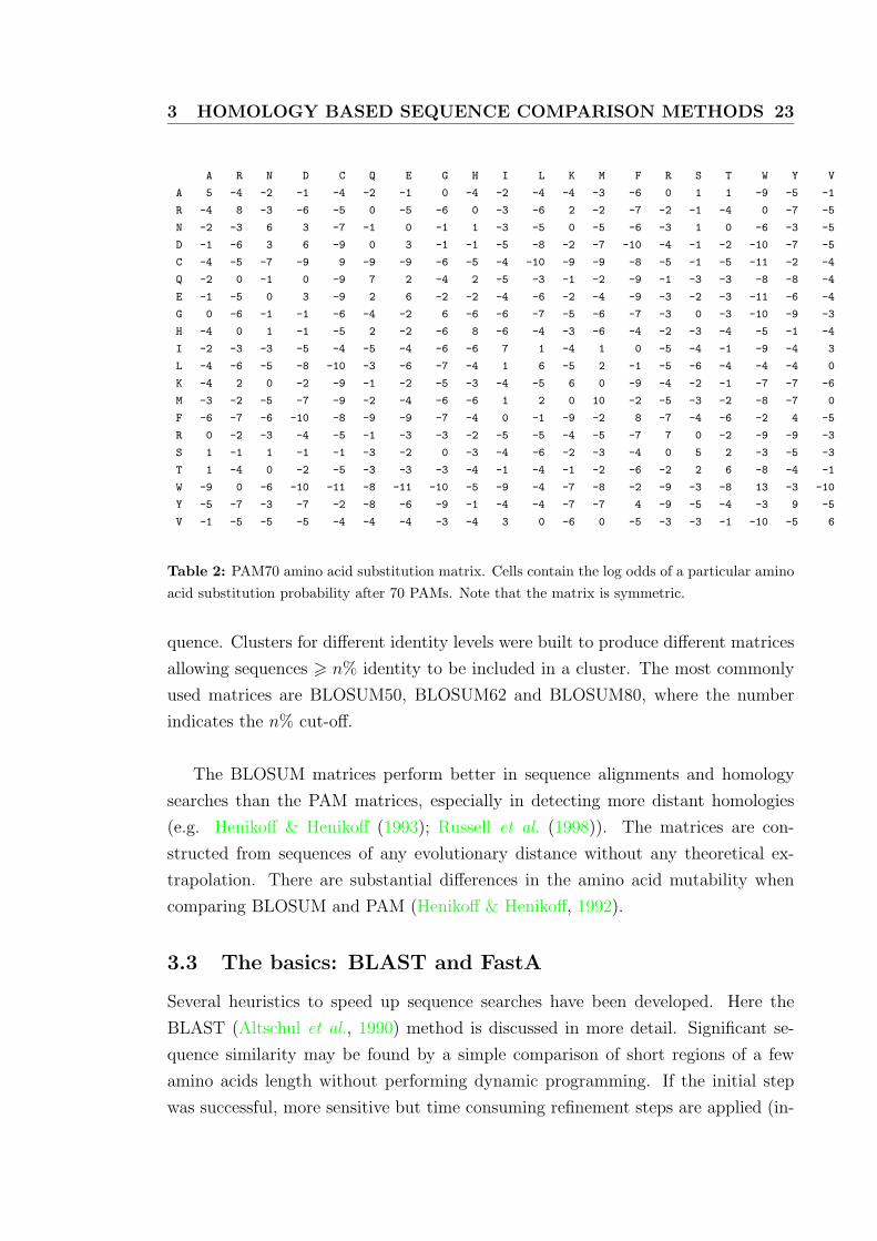
A 5 -4 -2 -1 -4 -2 -1 0 -4 -2 -4 -4 -3 -6 0 1 1 -9 -5 -1
R -4 8 -3 -6 -5 0 -5 -6 0 -3 -6 2 -2 -7 -2 -1 -4 0 -7 -5
N -2 -3 6 3 -7 -1 0 -1 1 -3 -5 0 -5 -6 -3 1 0 -6 -3 -5
D -1 -6 3 6 -9 0 3 -1 -1 -5 -8 -2 -7 -10 -4 -1 -2 -10 -7 -5
C -4 -5 -7 -9 9 -9 -9 -6 -5 -4 -10 -9 -9 -8 -5 -1 -5 -11 -2 -4
Q -2 0 -1 0 -9 7 2 -4 2 -5 -3 -1 -2 -9 -1 -3 -3 -8 -8 -4
E -1 -5 0 3 -9 2 6 -2 -2 -4 -6 -2 -4 -9 -3 -2 -3 -11 -6 -4
G 0 -6 -1 -1 -6 -4 -2 6 -6 -6 -7 -5 -6 -7 -3 0 -3 -10 -9 -3
H -4 0 1 -1 -5 2 -2 -6 8 -6 -4 -3 -6 -4 -2 -3 -4 -5 -1 -4
I -2 -3 -3 -5 -4 -5 -4 -6 -6 7 1 -4 1 0 -5 -4 -1 -9 -4 3
L -4 -6 -5 -8 -10 -3 -6 -7 -4 1 6 -5 2 -1 -5 -6 -4 -4 -4 0
K -4 2 0 -2 -9 -1 -2 -5 -3 -4 -5 6 0 -9 -4 -2 -1 -7 -7 -6
M -3 -2 -5 -7 -9 -2 -4 -6 -6 1 2 0 10 -2 -5 -3 -2 -8 -7 0
F -6 -7 -6 -10 -8 -9 -9 -7 -4 0 -1 -9 -2 8 -7 -4 -6 -2 4 -5
R 0 -2 -3 -4 -5 -1 -3 -3 -2 -5 -5 -4 -5 -7 7 0 -2 -9 -9 -3
S 1 -1 1 -1 -1 -3 -2 0 -3 -4 -6 -2 -3 -4 0 5 2 -3 -5 -3
T 1 -4 0 -2 -5 -3 -3 -3 -4 -1 -4 -1 -2 -6 -2 2 6 -8 -4 -1
W -9 0 -6 -10 -11 -8 -11 -10 -5 -9 -4 -7 -8 -2 -9 -3 -8 13 -3 -10
Y -5 -7 -3 -7 -2 -8 -6 -9 -1 -4 -4 -7 -7 4 -9 -5 -4 -3 9 -5
V -1 -5 -5 -5 -4 -4 -4 -3 -4 3 0 -6 0 -5 -3 -3 -1 -10 -5 6
Table 2: PAM70 amino acid substitution matrix. Cells contain the log odds of a particular aminoacid substitution probability after 70 PAMs. Note that the matrix is symmetric.
quence. Clusters for different identity levels were built to produce different matrices
allowing sequences > n% identity to be included in a cluster. The most commonly
used matrices are BLOSUM50, BLOSUM62 and BLOSUM80, where the number
indicates the n% cut-off.
The BLOSUM matrices perform better in sequence alignments and homology
searches than the PAM matrices, especially in detecting more distant homologies
(e.g. Henikoff & Henikoff (1993); Russell et al. (1998)). The matrices are con-
structed from sequences of any evolutionary distance without any theoretical ex-
trapolation. There are substantial differences in the amino acid mutability when
comparing BLOSUM and PAM (Henikoff & Henikoff, 1992).
3.3 The basics: BLAST and FastA
Several heuristics to speed up sequence searches have been developed. Here the
BLAST (Altschul et al., 1990) method is discussed in more detail. Significant se-
quence similarity may be found by a simple comparison of short regions of a few
amino acids length without performing dynamic programming. If the initial step
was successful, more sensitive but time consuming refinement steps are applied (in-

3 HOMOLOGY BASED SEQUENCE COMPARISON METHODS 24
cluding dynamic programming). Methods based on such simple comparisons are
heuristics and do not guarantee an optimal alignment between two sequences. Nev-
ertheless, when comparing a query sequence to a sequence database, generally most
of the sequences do not share any homology with the query, and may be skipped
by the fast heuristic step, reducing the search space to which the more detailed
comparisons are applied.
3.3.1 The FastA heuristic
Wilbur & Lipman (1983) introduced the first heuristic method to search a query
sequence against a database of sequences. This method has been subsequently im-
proved in the FastP and later in the FastA methods (Pearson & Lipman, 1988; Pear-
son, 1990). The FastA method can be applied to nucleotide or peptide sequences.
There are five major steps in the algorithm:
1. Identify matching ‘words’ between two sequences (the query and a database
sequence) that share identical pairs of amino acids (ktup = 2, a word of two
residues).
2. Find regions of high density of identities. This is done by finding the words
that are on the same diagonal of a plot between the two sequences. These
words are extended to merge with other existing words to form a region if the
distance of the previous word or region in residues is smaller than the score of
the current region or word match.
3. Re-score the ten highest scoring regions using a PAM250 matrix, and trim or
extend the ends of these to optimise their score. This is a partial alignment
without gaps.
4. If there are several regions above a given score cut-off, these regions are joined
via dynamic programming, producing a gapped alignment if their score can
be improved (the overall score is the sum of the scores of the regions minus a
penalty score for gaps). This score is called initn, and is used as a rank of the
database sequence.
5. For the top ranking sequences, a local alignment is constructed with the query
sequence using a centred 32 residue window on top of the best initn region.
The resulting score is the optimised score that is reported.
3 HOMOLOGY BASED SEQUENCE COMPARISON METHODS 25
The initial search step may not reduce the number of sequences substantially, but
it reduces the subsequent more detailed and time consuming searches to only a few
regions of the sequence that have to be compared in more detail. The calculation
of the initn value reduces the number of regions and sequences for which Smith-
Waterman local gapped alignments have to be produced. In summary, the FastA
method speeds up sequence database searches by reducing the time consuming dy-
namic programming to a set of matrices per sequence which are in total smaller
than the complete n×m matrix.
3.3.2 The BLAST heuristic
The original BLAST method (Basic Local Alignment Search Tool, Altschul et al.
(1990)) uses heuristics similar to FastA to find candidate sequences, but BLAST
is even faster then FastA. The original BLAST method produced un-gapped align-
ments and was refined (Altschul & Koonin, 1998; Schaffer et al., 2001) to gain more
sensitivity (including gapped alignments) and speed. The steps of the method im-
plemented in BLAST series 2.0 (Altschul & Koonin, 1998) for amino acid sequences
are described below (the steps for nucleotide sequences are similar).
1. Find word pairs of a given length (usually 3 residues for proteins) for which
the cumulative score is at least T . A word satisfying this condition is called a
hit. Scores are taken from a standard matrix such as BLOSUM or PAM.
2. If the two sequences contain at least two non-overlapping hits within a distance
A on the same diagonal then the extension of these matches is triggered. If
two hits overlap, the most recent one is ignored. This two-hit method reduces
the number of triggered extensions, which is the most time consuming step in
BLAST.
3. If the previous conditions are satisfied, the un-gapped bidirectional extension
of the second hit is triggered using the same substitution matrix as in the first
step. The extension terminates if its cumulative score cannot be improved
anymore, and the score is > S. A step in the heuristics to speed up the
extension procedure is to terminate an extension if it reaches another hit with
a score that falls a certain distance below the previous shorter extension. The
extended hit may include other hits. An extended hit is called an HSP (High
scoring Segment Pair).
3 HOMOLOGY BASED SEQUENCE COMPARISON METHODS 26
4. The highest scoring HSP with a score > Sg is further extended in both di-
rections via a gapped alignment. Only the highest scoring HSP is extended
because most of the HSPs will be included in this gapped extension.
5. The final alignment for hits for which a gapped extension produced a high
score are re-aligned with relaxed alignment parameters. This increases the
extend of the alignment.
BLAST performs far fewer local alignments compared to FastA and is therefore
much faster. Like FastA, gapped extensions are only performed on a relatively small
region within a sequence.
3.4 Basic statistics and probabilities for local alignments
The scoring system is crucial in distinguishing between real and chance alignments,
and equation 2 gives most of the basic statistics of a scoring system. Sequence search
methods employ a scoring system to judge whether similarity could have arisen by
chance, and for heuristics such as BLAST whether a more time consuming compar-
ison has to be performed.
The basic statistics for the score distributions from local ungapped alignments
has been described by Karlin and Altshul (Karlin & Altschul, 1990, 1993; Altschul
& Gish, 1996). The distribution of scores for hits between a real sequence and a
set of randomly generated sequences can be approximated with an extreme value
distribution. Scores as given in equation 2 are summed over the region participating
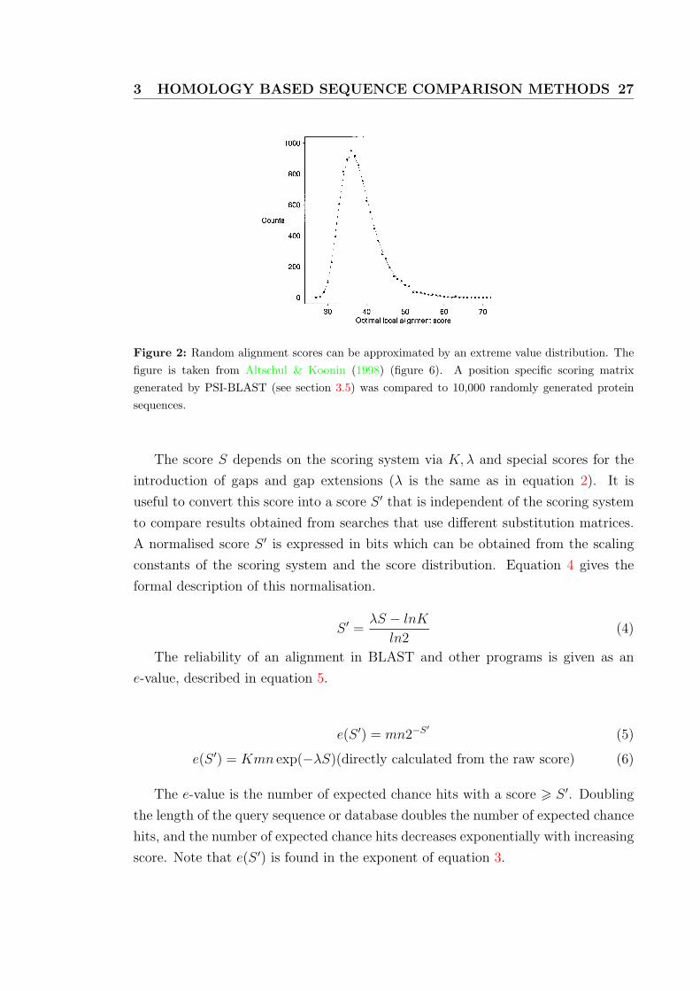
in a hit. Figure 2 shows scores that are approximated with an extreme value distri-
bution. Since this score distribution is the result of chance alignments, biologically
meaningful scores should be distributed at the long tail end of the distribution, and
the location of this score on the distribution can be treated as a confidence level for
this score (Karlin & Altschul, 1990). The formal description of this confidence is
given in equation 3 which is the probability to find at least one random alignment
with a score S > x. This probability is also known as a P -value. K is another
constant that depends on the scoring system, and mn is the product of the lengths
of the sequences that are compared. For database searches mn is the product of the
length of the query sequence and the search space of the database.
P (S > x) = 1− e−Kmne−λx (3)
3 HOMOLOGY BASED SEQUENCE COMPARISON METHODS 27 3397
Nucleic Acids Research, 1994, Vol. 22, No. 1Nucleic Acids Research, 1997, Vol. 25, No. 17 3397
Figure 6. The distribution of optimal local alignment scores from thecomparison of a position-specific score matrix with 10 000 random proteinsequences. The score matrix was constructed by PSI-BLAST from the 128 localalignments with E-value ≤0.01 found in a search of SWISS-PROT using asquery the length-567 influenza A virus hemagglutinin precursor (27) (SWISS-PROT accession no. P03435). The random sequences, each of length 567, weregenerated using the amino acid frequencies of Robinson and Robinson (20).Optimal local alignment scores were calculated using the position-specificmatrix in conjunction with 10 + k gap costs. The extreme value distribution thatbest fits the data (3,15) is plotted. A χ2 goodness-of-fit test with 34 degrees offreedom has value 41.8, corresponding to a P-value of 0.20.
lowest E-value found, as well as the number of shuffled sequencesyielding E-values ≤1 and 10. For comparison, we performed the
identical shuffled-database test on the gapped and originalversions of BLAST. To reduce the probability that high-scoringalignments were missed due to the heuristic nature of thealgorithms, we performed these tests with T = 9 rather than thedefault value of 11. The results are given in Table 2. For the 11queries, the median of the low PSI-BLAST E-values was 0.87,which corresponds to a median P-value of 0.58 (8,9). The meannumbers of shuffled database sequences with E-values <1 and 10were 1.0 and 8.7, respectively, within 20% of the expected valuesof 1.0 and 10.0. The equivalent tests for the ungapped and gappedversions of BLAST also yielded results that diverged from theoryby <50%.
The ability to estimate with reasonable accuracy the signifi-cance of gapped local matrix-sequence alignments permits us toautomate the construction of position-specific score matricesduring multiple iterations of the PSI-BLAST program. After eachiteration, we generate a new multiple alignment simply bycollecting those alignments with E-value lower than a definedthreshold. An interactive version of PSI-BLAST allows the userto override either the inclusion or exclusion of specific localalignments. Once a given database sequence has been used in thegeneration of a position-specific score matrix, low E-values forthis sequence are virtually guaranteed in future iterations, for thesequence is to a certain extent being compared with itself. Thebiological relevance of PSI-BLAST output thus depends criti-cally on avoiding the inappropriate inclusion of sequences in themultiple alignment constructed. Specifically, the utility of thescore matrix produced is immediately vitiated by the inclusion ofany alignment involving a region of highly biased amino acidcomposition (57,58).
Table 2. The comparison of various query sequences with a shuffled version of SWISS-PROT
Protein family SWISS-PROT Original BLAST Gapped BLAST PSI-BLASTaccession no. Low No. of seqs Low No. of seqs Low No. of seqsof query E-value with E-value E-value with E-value E-value with E-value
≤1 ≤10 ≤1 ≤10 ≤1 ≤10
Serine protease P00762 0.86 1 7 3.0 0 4 0.94 1 8
Serine protease inhibitor P01008 3.9 0 4 0.078 1 9 1.5 0 9
Ras P01111 3.4 0 8 3.4 0 7 1.1 0 9
Globin P02232 2.4 0 7 2.8 0 5 8.2 0 2
Hemagglutinin P03435 0.11 2 11 0.46 3 16 0.87 1 8
Interferon α P05013 2.4 0 6 0.27 2 4 0.11 2 11
Alcohol dehydrogenase P07327 1.5 0 2 0.80 1 5 1.5 0 9
Histocompatibility antigen P10318 0.91 1 7 0.13 1 7 0.0031 2 6
Cytochrome P450 P10635 0.84 2 5 8.5 0 3 0.46 1 15
Glutathione transferase P14942 1.0 1 10 3.3 0 3 0.30 2 9
H+-transporting ATP synthase P20705 0.012 1 8 0.26 2 14 0.79 2 10
Average (median or mean) 1.0 0.7 6.8 0.80 0.9 7.0 0.87 1.0 8.7
The original and gapped BLAST comparisons use BLOSUM-62 substitution scores (18). All three programs use threshold T parameter set to 9, but the gappedBLAST and PSI-BLAST programs use the two-hit method to trigger ungapped extensions. The original BLAST program has the X dropoff parameter set to nominalscore 23. The gapped BLAST and PSI-BLAST comparisons charge gaps of length k a cost of 10 + k. They have Xu set to 16, and Xg set to 40 for the database searchstage and to 67 for the output stage of the algorithms. Gapped alignments are triggered by a score corresponding to ∼22 bits. For PSI-BLAST, the query is first com-pared to the SWISS-PROT database, and the position-specific score matrix generated is then compared to a shuffled version of SWISS-PROT. The median is usedfor the average of the low E-values, and the mean otherwise.
Figure 2: Random alignment scores can be approximated by an extreme value distribution. Thefigure is taken from Altschul & Koonin (1998) (figure 6). A position specific scoring matrixgenerated by PSI-BLAST (see section 3.5) was compared to 10,000 randomly generated proteinsequences.
The score S depends on the scoring system via K,λ and special scores for the
introduction of gaps and gap extensions (λ is the same as in equation 2). It is
useful to convert this score into a score S ′ that is independent of the scoring system
to compare results obtained from searches that use different substitution matrices.
A normalised score S ′ is expressed in bits which can be obtained from the scaling
constants of the scoring system and the score distribution. Equation 4 gives the
formal description of this normalisation.
S ′ =λS − lnK
ln2(4)
The reliability of an alignment in BLAST and other programs is given as an
e-value, described in equation 5.
e(S ′) = mn2−S′
(5)
e(S ′) = Kmn exp(−λS)(directly calculated from the raw score) (6)
The e-value is the number of expected chance hits with a score > S ′. Doubling
the length of the query sequence or database doubles the number of expected chance
hits, and the number of expected chance hits decreases exponentially with increasing
score. Note that e(S ′) is found in the exponent of equation 3.

3 HOMOLOGY BASED SEQUENCE COMPARISON METHODS 28
Another confidence measure that requires a substantial sample of the score dis-
tribution is the z-score. It is defined as the distance of an the alignment score S from
the mean µ of the distribution of all scores of the analysis divided by the standard
deviation σ of the score distribution (score = (S − µ)/σ). The normalisation by
the standard deviation of the distribution ensures that even high scores with a short
distance to the mean get relative low z-scores if the score distribution is flat, e.g.
if there are many chance hits. A z-score is as defined above is only informative for
normally distributed scores. However, it is possible to calculate P-values for z-scores
that are derived from an extreme value distribution of scores (personal communica-
tion with William Pearson). Therefore z-scores may be used as confidence measures
for local alignments such as in the FastA (Pearson, 1990).
All equations in this section and equation 2 have only been proven to hold for
ungapped local alignments, but computational analysis and some analytical work
suggest the same applies to gapped local alignments (Karlin & Altschul, 1990, 1993;
Altschul & Gish, 1996; Altschul et al., 2001). Extreme value distributions fit scores
from gapped local alignments of randomly generated sequences well using standard
background frequencies (Robinson & Robinson, 1991) and a standard substitution
matrix such as BLOSUM62 with standard gap opening and extension scores (Wa-
terman & Vingron, 1994; Altschul & Koonin, 1998; Altschul & Gish, 1996), from
which the scale parameters λ and K are derived. These parameters cannot be deter-
mined analytically for gapped local alignments. However, Mott (2000) derived an
empirical formula from a large number of simulation with different scoring systems
to calculate λ. For ungapped local alignments these parameters are analytically
derived from the scoring system (Karlin & Altschul, 1990). The FastA method
generates enough optimal gapped local alignments between unrelated sequences for
each run to have a basis from which to λ and K can be estimated. The BLAST pro-
gram generates gapped alignments only for potentially related sequences and cannot
estimate the parameters from these scores. Therefore BLAST uses pre-estimated
parameters from simulations for different standard matrices and gap opening and
extension costs (Altschul et al., 1997).
3 HOMOLOGY BASED SEQUENCE COMPARISON METHODS 29
3.5 Sequence specific profiles and PSI-BLAST
As mentioned at the beginning of section 3.2, none of the standard substitution ma-
trices optimally describes the target frequencies of a particular class of sequences. A
position specific scoring matrix (PSSM) or sequence profile is specifically constructed
for a particular class of proteins. A PSSM has the dimensions n × 20, where n is
the length of the sequence. At each position ni of the matrix, a substitution score
for each of the 20 amino acids is given. The main difference to the standard substi-
tution matrices is that the score for the same amino acid type can differ depending
on the position within the sequence. Usually a PSSM is constructed from a multi-
ple sequence alignment, for example from a set of already identified homologues and
may be subsequently refined by pulling in more distant homologues when a database
is searched with the PSSM. Earlier profile methods (e.g. Patthy (1987); Gribskov
et al. (1987); Taylor (1986); Yi & Lander (1994); Tatusov et al. (1994)) used rather
complex procedures involving several programs with substantial user intervention.
The PSI-BLAST method (Altschul et al., 1997; Schaffer et al., 2001) combines all
the required steps, automatically constructs a PSSM and uses this profile to search
a sequence database. A comparison of several sequence database search methods
showed that PSI-BLAST is about three times more sensitive than BLAST or FastA
in detecting remote homologues (Park et al., 1998).
Figure 3 shows the basic steps of the PSI-BLAST procedure. First, a standard
BLAST, as described in section 3.3, is performed using a standard substitution ma-
trix (e.g. BLOSUM62) and a sequence database. From this run those sequences
satisfying a given e-value cut-off are stored, and a multiple sequence alignment is
constructed from these sequences. This multiple alignment is converted into a PSSM
which is then used in the second search round instead of the query sequence and
the standard substitution matrix to search the sequence database via the BLAST
algorithm. The difference between this step and the original BLAST is just that the
PSSM itself contains the information about the query sequence and the substitution
matrix. The procedure of searching the database and re-constructing a new PSSM
after every round is repeated until no more sequences with sufficient e-value can be
added to the list of sequences of the previous round or a given maximum number
of rounds has been reached. The result is a list of sequence alignments of the last
round that are of sufficient e-value.
3 HOMOLOGY BASED SEQUENCE COMPARISON METHODS 30
Position SpecificScoring Matrix (PSSM)
A R N D C ...1 M -2 -3 -4 -5 -2 ...2 N -3 -3 4 -7 -2 ...3 L -1 -4 -4 -5 -1 ...4 Y -4 -3 -4 -6 -4 ...5 D 0 0 -1 3 -3 ...6 L -1 -2 -5 -5 -1 ...
Convertto PSSM
Input/QuerySequence
New Sequence Hits
No Yes
BLASTsearch
ResultIterativesearch
Multiple SequenceAlignment
MNLYDLLELPTTASIKIAYRLA
Protein SequenceDatabase
List ofSequence Hits
List ofSequence Hits
create multiple sequence
alignment &purge highly similar
sequences
addto
Return
filter hits(E-value < x)
START
BLOSUM62
Figure 3: Overview of the PSI-BLAST procedure. The procedure starts by running BLAST fora query sequence against the sequence database using a standard matrix (here BLOSUM62). Inthe next round the PSSM, instead of the query sequence and the BLOSUM62 matrix, is used forthe database search. A new PSSM is constructed in every round until no new sequences can befound. A search cycle is called iteration. See text for more details.
3.5.1 Construction of a Position Specific Scoring Matrix
A multiple alignment is constructed by stacking all sequences found in a search
round with an e-value ≤ the cut-off. Sequences identical to the query are skipped,
and for sequences with very high sequence identity (> 97% in PSI-BLAST version
2.0 and > 93% in version 2.1) only one representative sequences is kept. The final
multiple sequence alignment M has residues or gap characters in every column and
row. For the calculation of the sequence weight for a column in the PSSM only
those rows (sequences) are considered that contribute a residue or gap to that row.
3 HOMOLOGY BASED SEQUENCE COMPARISON METHODS 31
Sequences contributing to a column of the multiple alignment are weighted in a
similar way as for the construction of the BLOSUM matrices described in (Henikoff
& Henikoff, 1992). Closely related sequences can bias the PSSM. This bias can be
avoided by weighting each sequence according to its individual information content.
Gaps are treated as the 21st distinct character of the amino acid alphabet, and any
column consisting of identical characters are ignored for calculating the individual
weight factor for a sequence. This weight scales the raw observed residue frequency
for a given column i of the PSSM, giving the weighted residue frequency fi. Fur-
ther the relative number of independent residue observations NC is calculated as
the mean of the number of different amino acid types observed at a position. The
maximum of NC is 21, but for most columns in the multiple alignment NC is much
smaller. NC is a per column scaling factor reflecting alignment variability.
A general frequency probability Qi/Pi with Q being the target frequency and P
being the standard background frequency on which equation 2 is based on is not
appropriate for the probability estimation for the PSSM, because of the weighting
issues discussed above. A small sample size (some alignments may just have a few
sequences at some columns) and the necessity for the prior knowledge of the relation-
ships among the residues requires a different probability scheme. The calculation of
Qi for a position in the PSSM includes the target frequency qij that was used for the
initial substitution matrix (see equation 2) to make use of the prior knowledge of the
residue relationships. Equation 7 calculates a pseudocount (Tatusov et al., 1994)
for a given column in the PSSM where qij is the target frequency for the standard
substitution matrix from equation 2.
gi =20∑j=1
fjPjqij (7)
Qi =αfi + βgiα + β
(8)
The target frequency Qi for a position in the PSSM is then given via equation
8 which combines the scaled observed frequency with the pseudocount. Therefore
a PSI-BLAST PSSM is a position specific scaled version of the initial substitution
matrix that was used. The factor α is defined as NC−1 to account for the alignment
variability mentioned above. The two equations above imply that for positions in
the query for which the multiple alignment does not have any sequences the initial
substitution score is used. The β factor can be used to increase or decrease the
3 HOMOLOGY BASED SEQUENCE COMPARISON METHODS 32
weight of the initial substitution matrix. Gaps do not have any position specific
scores, constant gap opening and gap extension scores are applied as for the standard
substitution matrices. The actual substitution score is calculated from Qi using
equation 2.
3.5.2 Applying BLAST to a position specific search
The BLAST method is applied in the same way to the PSSM as for a query se-
quence and a standard substitution matrix, assuming the same statistics holds for a
position specific search. The calculation of the normalised score S ′ for hits includes
the scaling parameters λ and K for which Altschul et al. use the same values as for
the initial substitution matrix that was used in the first round (e.g. BLOSUM62).
They showed that the employed scoring system fits well the observed score distribu-
tion. The score distribution from comparisons of random sequences with a PSSM
derived from a real sequence can be fitted by an extreme value distribution (figure
2) with the calculated parameters λ and K close to those for gapped simulations for
a BLOSUM62 matrix.
By employing the pseudocount PSI-BLAST makes use of the statistics from
BLAST and the underlying substitution matrix which assumes a standard amino
acid composition of the query sequence and the database. Although the initial anal-
ysis of PSI-BLAST has shown that its statistics fits the observed score distribution,
and the calculation of the e-value approximates the observed error rate within a
range of 20%, there have been problems with the PSI-BLAST statistics for a range
of query sequence the more the sequence differs from the assumed standard amino
acid composition. A BLAST comparison between a query and a database sequence
of similar biased composition may produce a hit with significantly high score be-
cause the standard BLAST statistics does not apply for this sequence pair. Recent
changes in the BLAST and PSI-BLAST algorithms (Schaffer et al., 2001) imple-
mented in the 2.1 series of the program consider biased amino acid compositions.
Especially for PSI-BLAST, biased sequences have a strong impact because in every
iteration the PSSM itself will be biased towards the amino acid composition of the
query, producing even more unreliable results in the next search round (Schaffer
et al., 2001; Altschul & Koonin, 1998).
The most important change to cope with different amino acid compositions is a

3 HOMOLOGY BASED SEQUENCE COMPARISON METHODS 33
PSSM specific λ. For composition biased sequence pairs the standard λ (e.g. that
for the BLOSUM62 scoring system) is generally too big and results in a lower e-
value (lower e-values give more confidence) than justified (Schaffer et al., 2001). A
composition dependant λ′ is therefore generally smaller than the standard λ. It is
computationally too intensive to estimate λ′ by fitting the score distribution for each
query or PSSM and database sequence pair. Since λu can be determined analytically
(Karlin & Altschul, 1990) for ungapped alignments (it is the unique solution to sum
the scores for a matrix colum given in equation 2 to one), a composition specific λ′ufor scores from ungapped alignments is calculated using the amino acid frequencies
of the database sequence and the query. The composition rescaled score for a matrix
cell in the PSSM is then given by λ′uλuSij, where Sij is the non-scaled score of the
PSSM.
As mentioned in section 3.4 the statistics for ungapped alignments has been
shown to approximate score distributions for gapped alignments, too. Matrix rescal-
ing is time consuming because it has to be performed for every query database se-
quence pair. Rescaling is only triggered if an alignment produces a significantly high
score using the non-scaled scoring system. The alignment for the sequence pair (or
a PSSM and the sequence) is then recalculated. e-Values as the common confidence
measure for BLAST and PSI-BLAST alignments are more conservative with the
rescaled scoring system and have been shown to be more realistic than the original
e-values (Schaffer et al., 2001).
To avoid the application of the BLAST algorithm to highly biased sequences
with a low amino acid entropy, for which re-scaling may not be sufficient to stop
a corrupted search, a low complexity filter can be applied to remove regions from
the database or query sequence that differ markedly from the standard amino acid
composition. Positions in these low complexity regions are replaced by the ‘X’ char-
acter and are ignored by the BLAST search procedure. Such a filter is implemented
in the BLAST 2.0 and 2.1 series (Wootton, 1994).
Finally, it is worth mentioning that the sensitivity of PSI-BLAST, the ability
to detect even distantly related homologues, depends on the diversity and size of
the sequence database that is used for the search. Generally in every iteration
more distantly related sequences are identified and added to the PSSM. After every
round the PSSM explores evolution a step backward. PSI-BLAST would not be
3 HOMOLOGY BASED SEQUENCE COMPARISON METHODS 34
able to detect the relationship between a query sequence A and a distantly related
sequence B in the database if there were no evolutionary intermediates present in
the database, see e.g. Aravind & Koonin (1999).
3.6 Using sequence profiles with IMPALA
The IMPALA method (Schaffer et al., 1999) compares a query sequence against a
library of PSSM produced by PSI-BLAST. This is particularly useful if one wants
to find the protein or domain family to which a given query belongs. Each family
is represented as one PSSM in the library. Such a library may be constructed by
searching a large sequence database with a member of a characterised protein family
using PSI-BLAST. The final PSSM produced by PSI-BLAST may then be used as
a representation of the protein family.
The comparison of the query sequence with each PSSM is performed via the
Smith-Waterman procedure (see equation 1 and text in that section), so that optimal
local alignments are guaranteed. The time consuming Smith-Waterman procedure is
acceptable because a profile library generally contains only a few hundred members
representing families or domains rather than hundreds of thousands of single protein
sequences from a database that is used within e.g BLAST and PSI-BLAST searches.
IMPALA faces the same statistical problems calculating significance for scores be-
tween the query and a PSSM as PSI-BLAST. In fact the re-scaling procedure to
scale a PSSM by λ′u (mentioned in the previous section) was initially developed for
IMPALA and later adapted by PSI-BLAST version 2.1. IMPALA performs similarly
to PSI-BLAST version 2.0 and 2.1 in terms of sensitivity and error rate. Since IM-
PALA and PSI-BLAST version 2.1 use the same re-scaled scoring system, e-values
are very similar, whereas e-values generally differ from those calculated by the older
PSI-BLAST version 2.0.
A recent development is the RPS-BLAST program (Reversed Position Specific,
Marchler-Bauer et al. (2002)) that is a derivative of IMPALA. The query is compared
to the query PSSM via the BLAST heuristics instead of using a Smith-Waterman
dynamic programming as in IMPALA (the program is part of the NCBI BLAST
package).
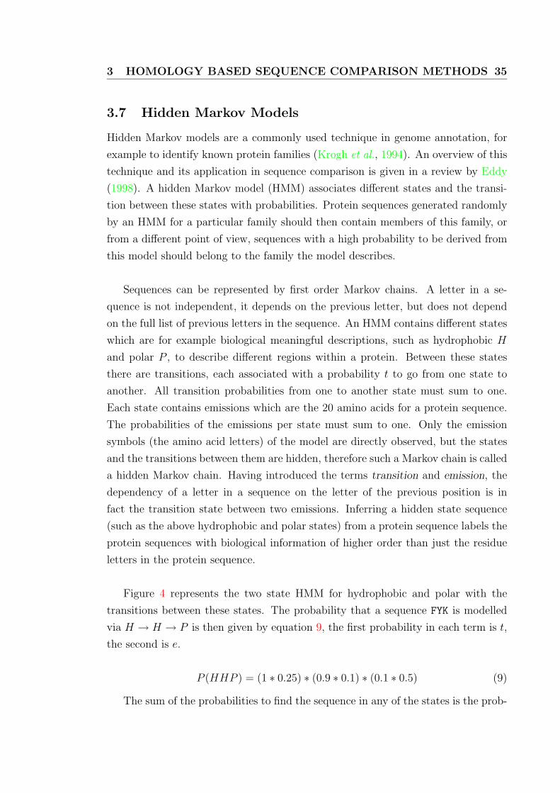
3 HOMOLOGY BASED SEQUENCE COMPARISON METHODS 35
3.7 Hidden Markov Models
Hidden Markov models are a commonly used technique in genome annotation, for
example to identify known protein families (Krogh et al., 1994). An overview of this
technique and its application in sequence comparison is given in a review by Eddy
(1998). A hidden Markov model (HMM) associates different states and the transi-
tion between these states with probabilities. Protein sequences generated randomly
by an HMM for a particular family should then contain members of this family, or
from a different point of view, sequences with a high probability to be derived from
this model should belong to the family the model describes.
Sequences can be represented by first order Markov chains. A letter in a se-
quence is not independent, it depends on the previous letter, but does not depend
on the full list of previous letters in the sequence. An HMM contains different states
which are for example biological meaningful descriptions, such as hydrophobic H
and polar P , to describe different regions within a protein. Between these states
there are transitions, each associated with a probability t to go from one state to
another. All transition probabilities from one to another state must sum to one.
Each state contains emissions which are the 20 amino acids for a protein sequence.
The probabilities of the emissions per state must sum to one. Only the emission
symbols (the amino acid letters) of the model are directly observed, but the states
and the transitions between them are hidden, therefore such a Markov chain is called
a hidden Markov chain. Having introduced the terms transition and emission, the
dependency of a letter in a sequence on the letter of the previous position is in
fact the transition state between two emissions. Inferring a hidden state sequence
(such as the above hydrophobic and polar states) from a protein sequence labels the
protein sequences with biological information of higher order than just the residue
letters in the protein sequence.
Figure 4 represents the two state HMM for hydrophobic and polar with the
transitions between these states. The probability that a sequence FYK is modelled
via H → H → P is then given by equation 9, the first probability in each term is t,
the second is e.
P (HHP ) = (1 ∗ 0.25) ∗ (0.9 ∗ 0.1) ∗ (0.1 ∗ 0.5) (9)
The sum of the probabilities to find the sequence in any of the states is the prob-

3 HOMOLOGY BASED SEQUENCE COMPARISON METHODS 36
H Pt = 0.9
t = 0.05
t = 0.1
t = 0.95
F = 0.25Y = 0.10K = 0.01
...
F = 0.01Y = 0.05K = 0.50
...
e e
Figure 4: Schematic representation of a two state hidden Markov model, to assign a residue in aprotein sequence to either the hydrophobic H or the polar P state. t is the transition probability,e gives the probability for emitting a particular amino acid type from this state.
ability with which the sequence can me modelled by this HMM. Usually dynamic
programming is used to find the optimal path for a given input sequence through the
HMM, where the rows and the columns of the matrix contain the sequence letters
and the states.
HMMs are used in a wide range of bioinformatics applications, such as (i) gene
prediction where a gene is modelled with different states such as exon-intron struc-
ture (see section 2.1), (ii) transmembrane helix prediction of protein sequences (e.g.
Sonnhammer et al. (1998); Krogh et al. (2001); Tusnady & Simon (2001)) where a
helix may get states for the helix caps and states for the hydrophobic core and (iii)
the identification of homologous sequence families (Bateman et al., 1999). Homol-
ogy based sequence searches using carefully constructed HMMs for protein families
perform better than PSI-BLAST (Park et al., 1998) in detecting distantly related
proteins, but the construction of high quality HMMs on which the performance re-
lies is difficult and usually requires several steps and manual inspection (Bateman
et al., 1999, 2002; Letunic et al., 2002; Gough & Chothia, 2002). The key aspect for
the performance of any HMM based application is the design of the HMM which
includes a definition of the states and the associated probabilities e and t.
Profile HMMs that describe a protein or domain family such as in PFAM and
SMART (see section 2.3.4) usually derive the probabilities for e and t from multi-
4 PROTEIN STRUCTURE AND GENOME ANNOTATION 37
ple sequence alignments. An initial HMM is constructed that may just contain a
limited number of rather closely related members of the family. This HMM is then
iteratively refined in a similar way PSI-BLAST refines its PSSMs (Bateman et al.,
1999). A HMM in database search round n will detect more divergent members of
the family than in round n− 1, and the new HMM that is constructed after round
n is used to search the sequence database in round n + 1. The most commonly
used profile HMM packages are HMMer (Eddy, 1998) and SAMT99 (Karplus et al.,
1998). These methods contain programs to construct, refine and manage HMMs
and to search libraries of HMMs with a query sequence.
The states for a sequence profile HMM are (a) the residue positions of the protein
family (from one to the sequence length of members of the family), referred to as
match states, (b) a deletion state between each match state that allows bypassing
a match, and (c) an insertion state between each match state to allow residues to
be inserted between two matches. Figure 5 represents a model for a three residue
sequence motif (Eddy, 1998). The two major differences between sequence profiles
such PSI-BLAST PSSMs and HMMs is that a PSSM does not score gaps in a posi-
tion specific way whereas a HMM contains the deletion (gaps) state. Further, in a
HMM a state is dependant on the previous state, whereas a position in a PSSM is
mathematically independent.
4 Protein structure and genome annotation
This section explains why knowledge of the three dimensional structure of proteins
is important. There is a huge discrepancy between the availability of protein se-
quences and their 3D-structures. Currently there are more than 800,000 different
sequences in the public databases (12/2001, ftp://ftp.ncbi.nlm.nih.gov/blast/db/),
but there are less than 16,000 experimentally determined protein structures in the
Protein Data Bank (PDB, 12/2001, http://www.rcsb.org, Berman et al. (2000)),
and these contain redundancies such as structures with point a mutation. Despite
the difference in absolute numbers, the sequence and the structure databases both
grow exponentially.

4 PROTEIN STRUCTURE AND GENOME ANNOTATION 38
i1
d1
m1
i0
b e
i2
d2
m2
i3
d3
m3
CCCCC
1
AGDVK
2
FWYFY
3
X X XX
C X FY�
Figure 5: A small profile HMM (right) representing a short multiple alignment of five sequences(left) with three consensus columns. The three columns are modelled by three match states (squareslabelled m1, m2 and m3), each of which has 20 residue emission probabilities, shown with blackbars. Insert states (diamonds labeled i0-i3) also have 20 emission probabilities each. Delete states(circles labeled d1-d3) are ‘mute’ states that have no emission probabilities. A begin and end stateare included (b, e). State transition probabilities are show as arrows. The figure and the legendare from Eddy (1998) (figure 2).
4.1 Functional and evolutionary insights from protein struc-
ture
The 3D-structure of a protein determines its biochemical function. Homology based
sequence comparisons and motif searches to identify the function of a protein are
therefore simplifications because these searches only consider 1D-information. How-
ever, divergent sequences often share a similar 3D-structure that accepts to some
extent a range of amino acid substitutions. The 3D-structure is generally more
conserved than the 1D-structure (the sequence), see e.g. Chothia & Lesk (1986)
and Murzin et al. (1995). Figure 6 shows the dependency of the structural sim-
ilarity measured as the root mean square of Cα distances of homologous protein
domains and the sequence identity between these domain pairs. At about 20-25%
sequence identity the 3D-similarity starts to decrease dramatically. Distantly re-
lated sequences with less than 20% sequence identity (the twilight zone) generally
only share a similar structural scaffold, a common fold, with differences in struc-
tural details which usually determine the biochemical function (Hegyi & Gerstein,
1999; Wilson et al., 2000). However, an analysis from Wood & Pearson (1999) using
z-scores for a sequence-structure comparison showed a linear relationship between
z-scores of the sequences members of a fold and the z-scores of their structural align-
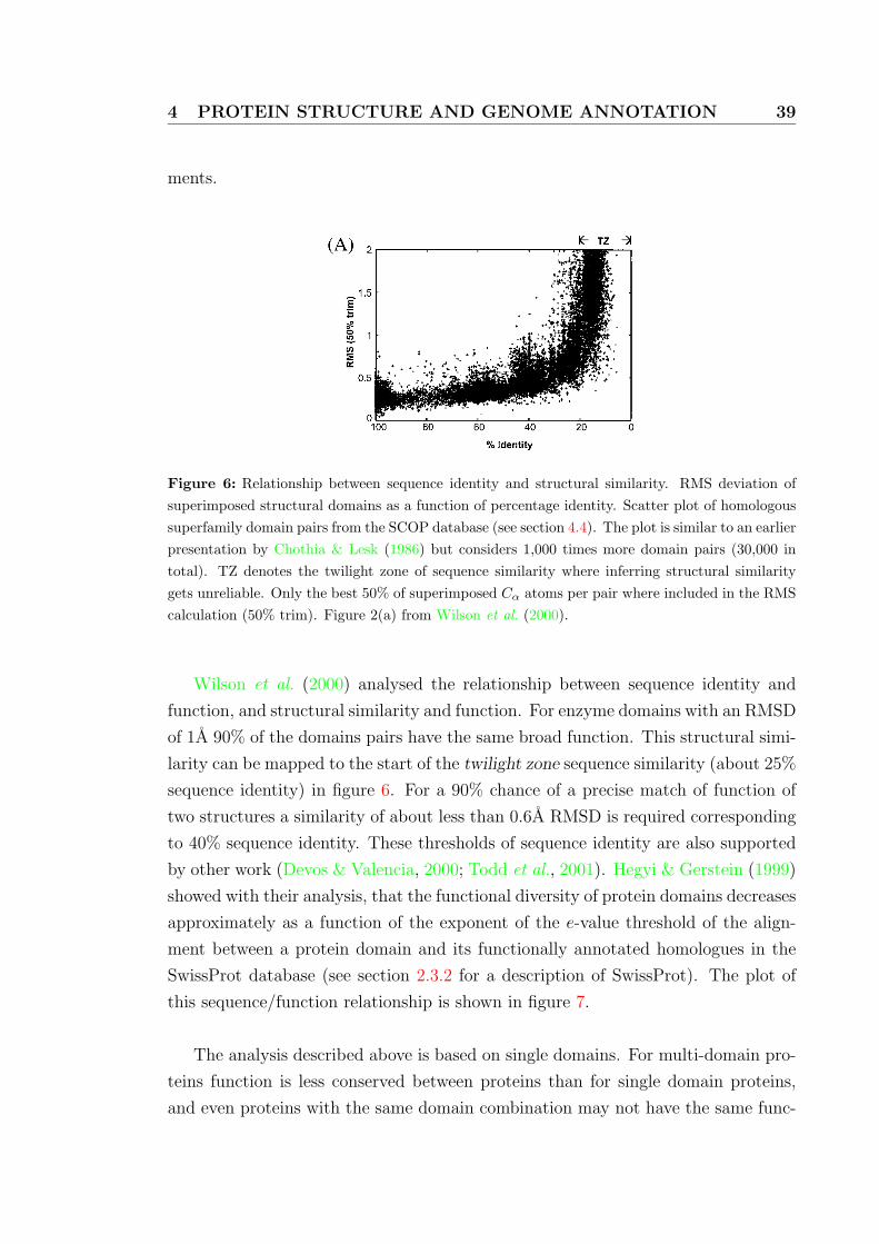
4 PROTEIN STRUCTURE AND GENOME ANNOTATION 39
ments.
in the twilight zone (according to the percent iden-tity to Pseq calibration in Figure 4(b)), structuralsimilarity is more signi®cant than sequence simi-larity (having a smaller P-value or more negativelog P-value). In contrast, for pairs with more than�30 % identity, the situation is reversed, with agiven pair having more signi®cant sequence simi-larity than structural similarity. One possibleinterpretation of this reversal is as follows. Struc-ture is always more highly conserved thansequence, so usually a given amount of structuralsimilarity is not as signi®cant as a correspondingamount of sequence similarity. However, this istrue only when meaningful sequence similarity
actually exists; thus, it does not apply in the twi-light zone, where sequence similarity is by de®-nition not signi®cant. Note that all pairs in ourcomparison share at least the same fold, implyingthat they always have a signi®cant amount ofstructural similarity.
In other words, for closely related sequences,differences in sequence similarity are more mean-ingful, whereas for highly diverged sequences thatshare the same fold, the differences in structuralsimilarity are more signi®cant.
Fitting two lines to the Pstr versus Pseq graphsuggests that the same might be done for otherscoring schemes. It is possible to some degree to ®t
Figure 2. RMS as a function of percent identity. (a) A simple scatter plot of our pairs, relating RMS separation topercent sequence identity. This is similar to the presentation given by Chothia & Lesk (1986), but in this survey welooked at 30,000 pairs, 1000 times the number they compared. Outliers (pairs with RMS scores further than two stan-dard deviations from the mean for their percent identity) are excluded from this graph; they represent domains thatare very closely related with the exception of a conformational change. (b) A simpli®ed graph with a number of ®tsto the data. For each percent identity bin we show the median RMS value, indicated by (^) and the top and bottomquartile RMS values, indicated by the bars. Two ®ts are drawn through the median RMS values. The thin line,labeled SINGLE, is a simple exponential ®t through the medians. It has the form:
R � 0:21e0:0132H
where R is the RMS deviation after least-square ®tting, H is the percent difference between the sequences (H forHamming distance), and H � 100 % ÿ I, where I is the percent sequence identity. The thick line, labeled MULTI, is amultigraph ®t, which is described in the legend to Figure 4. The relation between RMS and percent identity accordingto this ®t is expressed by the equation:
R � 0:18e0:0187H
The twilight zone of sequence identity and below is labeled TZ. In this region, sequence similarity is not signi®cantand not reliable for predicting structural similarity. This is why the median values in this area of the graph deviatesigni®cantly from the ®ts, which consider only data above 20 % sequence identity. For reference we include the orig-inal data points from Chothia and Lesk's, 1986 paper (A.M. Lesk, personal communication), indicated by X. Theirdata follow the form:
R � 0:40e0:0187H
The difference between the Chothia & Lesk trend and our relationship is due to the different trimming methods usedin calculating the RMS score. Chothia and Lesk imposed a 3 AÊ cut-off in determining the conserved core residues; wede®ned the core as the better matching (in terms of Ca distances) half (50 %) of the residue pairs. (c) and (d) Theeffect our trimming has on median RMS values. The RMS values in (c) are calculated from all the matched residuesin each pair; the values in (d) are calculated from the better matching 50 % of the residues.
238 Assessing Annotation Transfer for Genomics
Figure 6: Relationship between sequence identity and structural similarity. RMS deviation ofsuperimposed structural domains as a function of percentage identity. Scatter plot of homologoussuperfamily domain pairs from the SCOP database (see section 4.4). The plot is similar to an earlierpresentation by Chothia & Lesk (1986) but considers 1,000 times more domain pairs (30,000 intotal). TZ denotes the twilight zone of sequence similarity where inferring structural similaritygets unreliable. Only the best 50% of superimposed Cα atoms per pair where included in the RMScalculation (50% trim). Figure 2(a) from Wilson et al. (2000).
Wilson et al. (2000) analysed the relationship between sequence identity and
function, and structural similarity and function. For enzyme domains with an RMSD
of 1A 90% of the domains pairs have the same broad function. This structural simi-
larity can be mapped to the start of the twilight zone sequence similarity (about 25%
sequence identity) in figure 6. For a 90% chance of a precise match of function of
two structures a similarity of about less than 0.6A RMSD is required corresponding
to 40% sequence identity. These thresholds of sequence identity are also supported
by other work (Devos & Valencia, 2000; Todd et al., 2001). Hegyi & Gerstein (1999)
showed with their analysis, that the functional diversity of protein domains decreases
approximately as a function of the exponent of the e-value threshold of the align-
ment between a protein domain and its functionally annotated homologues in the
SwissProt database (see section 2.3.2 for a description of SwissProt). The plot of
this sequence/function relationship is shown in figure 7.
The analysis described above is based on single domains. For multi-domain pro-
teins function is less conserved between proteins than for single domain proteins,
and even proteins with the same domain combination may not have the same func-

4 PROTEIN STRUCTURE AND GENOME ANNOTATION 40
Figure 7: Multi-functionality of protein domains versus e-value threshold. A domain has multiplefunctions if at least two homologues of different function from the SwissProt database can beidentified for this domain. The e-value of the alignment between homologous pairs is plotted asthe negative logarithm to the base of 10 against the fraction of domains with multiple functions(i.e. increasing values on the x-axes indicates more confidence in the homologous relationship).Starting from an e-value of 10−5 (log10 − 5) multi-functionality decreases exponentially. Figure 7from Hegyi & Gerstein (1999).
tion (Hegyi & Gerstein, 2001). This renders functional flexibility of folds of domains
in a different context.
The relationship between structure and function raises the question whether
there is a relationship between a particular function and a fold. Studies from Mar-
tin et al. (1998) showed only little preference of a function to be associated with
a particular protein fold. However, other results (Hegyi & Gerstein, 1999; Wilson
et al., 2000) show a significant bias of certain folds with a particular group of func-
tions. E.g., mixed α/β-folds are often associated with enzymatic domains whereas
all-α domains are biased towards non-enzymatic function. On the other hand there
are a few folds such as the TIM (Triose-phosphate Isomerase) barrel that provides
a generic scaffold to fulfil a broad range of enzymatic functions.
Todd et al. (2001) showed that 25% of the homologous superfamilies of simi-
lar structure have different enzymatic function, highlighting the divergent evolution
within these superfamilies. Most functional changes within a related set of sequences
are due to a change in the substrate but maintain the same reaction mechanism
(Holm & Sander, 1997; Todd et al., 2001).
Due to the structural conservation of proteins the number of distinct 3D-archi-
tectures for globular proteins has been estimated to be limited between 1,000 and

4 PROTEIN STRUCTURE AND GENOME ANNOTATION 41
7,000 (Brenner et al., 1997; Govindarajan et al., 1999; Zhang & DeLisi, 1998; Wolf
et al., 2000). This means that many proteins have the same or a very similar general
architecture of secondary structure elements (α-helices and β-sheets), although their
peptide sequences may not show obvious similarity. Considering this structural ‘lim-
itation’, functional diversity has to be generated by adopting an existing structural
scaffold to a particular function. Functional changes within the same structural fold
is often related to critical local sequence changes Todd et al. (2001); Aloy et al.
(2001), and in difficult cases may be traced to differences of a few critical atoms.
An overview about the relationships between sequence, structure, function and
evolution is given by Orengo et al. (1999); Thornton et al. (1999, 2000). Generally
protein structure is more conserved than its function (and its sequence).
4.2 Examples for protein structure/function relationships
4.2.1 Glycogen synthase kinase 3β
The recently published structure of the glycogen synthase kinase 3β (GSK3β, Dajani
et al. (2001)) is represented as an example of how protein structure reveals insight
into biochemical function, supporting and guiding functional studies. The GSK3β
plays a regulatory role in two distinct signalling pathways, the insulin induced sig-
nalling pathway to regulate glycogen synthesis and the Wnt (Wintbeutel) signalling
pathway involved in cell proliferation and development. The default for GSK3β is
to phosphorylate and thereby inhibit its target proteins.
GSK-3β contains an N-terminal activation segment that is also found in other
kinases such as ERK2 MAP kinase (Zhang et al., 1995), forming a β barrel structure
that opens a substrate specific binding cleft and positions the active site residues
for the phosphorylation reaction. This activation itself is enhanced by the phospho-
rylation of the activation segment (tyrosine 216 in GSK-3β). A feature specific for
GSK3β is the P+4 phosphorylation pattern. The kinase efficiently phosphorylates
substrates at a position with a serine or threonine if the residue 4 positions towards
the C-terminus has already been phosphorylated (primed phosphorylation). Addi-
tional serine or threonine residues can be phosphorylate in +4 steps in a C-terminal
to N-terminal direction (hyper-phosphorylation, Fiol et al. (1994)).
The crystal structure was analysed to suggests a model by which the requirement

4 PROTEIN STRUCTURE AND GENOME ANNOTATION 42
for primed phosphorylation and the substrate specificity is explained. The struc-
ture of GSK3β shows the active from of the protein, with an open cleft between
the activation segment at the N-terminus and the C-terminal domain. Figure 8 (A)
shows the surface of GSK3β with the functionally key residues labelled. The cleft
from the positively charged patch formed by R96, R80 and K205 to the left, passing
the active site residues R220 and D181, is the substrate binding site. The positively
charged patch is stabilised by either a phosphorylated tyrosine at position 216 form-
ing a hydrogen bonding network with the three positively charged residues or by a
free phosphate or sulphate from the surrounding buffer in vitro (as it is found in the
crystal structure) and the cytosol in vivo. The modelled protein substrate complex
in 8 (B) explains the requirement for P+4 primed substrates, and the specificity for
substrates containing a serine or threonine at ‘P(0)’ and ‘P(+4)’.
A B
Figure 8: GSK3β surface and active site. From Dajani et al. (2001), figures 3a and 4a. (A) Thesolvent-accessible surface of GSK3β coloured according to electrostatic potential (red, negative,blue: positive). The intensive positive patch generated by the basic side chains of Arg 96, Arg180 and Lys 205 is indicated, as is the location of the catalytic Asp 181 and Arg 220 which couldinteract with a phosphorylated Tyr 216. The N-terminal mainly neutral activation segment islocated towards the bottom of figure. (B) Phospho-Substrate bind model. Model of substratebinding (peptide sequence PPSPSLS) to GSK3β. Phosphorylation of a serine at P(0) by the activesite residues (red) depends on a ‘priming’ phospho-serine at P(+4) interacting with residues ofthe positively charged patch (blue sidechains) shown in (A) fitting the substrate into the bindingpocket.
The authors further suggest an autoinhibition mechanism to interpret the inhibi-

4 PROTEIN STRUCTURE AND GENOME ANNOTATION 43
tion of GSK3β when serine 9 is phosphorylated in the insulin pathway (Cross et al.,
1995). The 35 residue N-terminal peptide, which is distorted in the crystal structure
and therefore not visible, was modelled into the substrate binding site serving as a
pseudo primed substrate analogue with the phosphorylated serine 9 as ‘P(+4)’ and
a proline 5 in ‘P(0)’ occupying the pocket at the catalytic residues. The authors
showed experimentally that inhibition depends on the sequence context of the serine
9, and is in fact specific to the sequence N-terminal fragment of GSK3β itself.
The structure of GSK3β from Dajani et al. (2001) does not reveal any insights
into how GSK3β acts differently in the two signalling pathways (insulin and Wnt).
However, recently a structure of a complex between GSK3β and a peptide from
an interacting regulatory protein required in the Wnt pathway was published (Bax
et al., 2001), showing that the interaction site is close to the substrate binding site
but without any overlap. This structural complex explains why GSK-3β can be
inhibited in the Wnt pathway while staying active in the insulin pathway.
4.2.2 Similar structure and function - different sequence
As figure 6 shows and is further discussed in section 4.3 below, similar sequences
generally have a similar 3D-structure which in turn determines the biochemical func-
tion of the protein, although, as explained in section 4.1, it is not straightforward
to identify these relationships. In this section two protein structures with such a
difficult relationship are discussed.
The structures of the core domain from different viral integrase proteins Dyda
et al. (1994) are similar to ribonuclease H (RNaseH, Katayanagi et al. (1990); Davies
et al. (1991)), but their sequences do not show significant similarity (Yang & Steitz,
1995; Dyda et al., 1994). The integrase inserts the viral DNA into the host DNA,
whereas RNaseH hydrolyses RNA strands of RNA-DNA hybrids. Despite the differ-
ence of their biological function, both enzymes perform a similar trans-esterifiaction
reaction that requires either Mg2+ or Mn2+ ions and three carboxylates. Overall
the reaction mechanism of both enzymes has been proposed to be similar Yang &
Steitz (1995).
The topology of the core folds for the integrase and the RNaseH are the same,
but the length and twist of the secondary structure elements are different, also both

4 PROTEIN STRUCTURE AND GENOME ANNOTATION 44
folds contain additional secondary structure elements. Figure 9 shows a superpo-
sition of both structures. The three residues of the catalytic site that provide the
carboxylates for the chelated metal-ion are in similar relative positions (coloured in
magenta and green). In integrase glutamate 157 (magenta) does not interact di-
rectly with the magnesium-ion, although mutagenesis has shown that this position
requires a glutamate (Kulkosky et al., 1992). Further, glutamate 157 is in an oppo-
site position relative to glutamate 48 of the RNaseH. It has to be pointed out that
the fold of the Avian Sarcoma Virus (ASV) integrase shown in the figure is similar
to the HIV-1 integrase (Bujacz et al., 1996) with a sequence identity of 24% but the
relative orientation of the three active site residues are different (Bujacz et al., 1996).
A B
Figure 9: Superposition of ribonuclease H from E. coli (PDB code 1RDD, red structure,Katayanagi et al. (1993)) and integrase from Avian Sarcoma virus (PDB code 1VSD, structureshown in blue, Bujacz et al. (1996)). (A) The RMSD of the superposition is 3.9A. Most similarityis found in the 5 stranded sheet, both structures contain additional secondary structure elements,although their general topology is the same. (B) Mg2+ binding site of both enzymes (integrasein magenta, and RNaseH in green). The two aspartates occupy similar positions whereas the twoglutamates are on opposite sites of the metal ion.
The similarity between both protein domains and the proposal of a common
enzymatic mechanism was identified only because their 3D-structures are available,
pointing out the limitations of sequence based comparisons, and raising the question
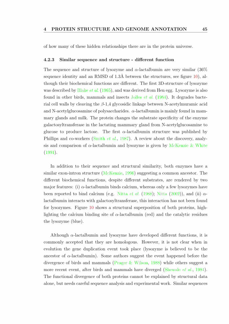
4 PROTEIN STRUCTURE AND GENOME ANNOTATION 45
of how many of these hidden relationships there are in the protein universe.
4.2.3 Similar sequence and structure - different function
The sequence and structure of lysozyme and α-lactalbumin are very similar (36%
sequence identity and an RMSD of 1.3A between the structures, see figure 10), al-
though their biochemical functions are different. The first 3D-structure of lysozyme
was described by Blake et al. (1965), and was derived from Hen egg. Lysozyme is also
found in other birds, mammals and insects Jolles et al. (1984). It degrades bacte-
rial cell walls by cleaving the β-1,4 glycosidic linkage between N-acetylmuramic acid
and N-acetylglucosamine of polysaccharides. α-lactalbumin is mainly found in mam-
mary glands and milk. The protein changes the substrate specificity of the enzyme
galactosyltransferase in the lactating mammary gland from N-acetylglucosamine to
glucose to produce lactose. The first α-lactalbumin structure was published by
Phillips and co-workers (Smith et al., 1987). A review about the discovery, analy-
sis and comparison of α-lactalbumin and lysozyme is given by McKenzie & White
(1991).
In addition to their sequence and structural similarity, both enzymes have a
similar exon-intron structure (McKenzie, 1996) suggesting a common ancestor. The
different biochemical functions, despite different substrates, are rendered by two
major features: (i) α-lactalbumin binds calcium, whereas only a few lysozymes have
been reported to bind calcium (e.g. Nitta et al. (1988); Nitta (2002)), and (ii) α-
lactalbumin interacts with galactosyltransferase, this interaction has not been found
for lysozymes. Figure 10 shows a structural superposition of both proteins, high-
lighting the calcium binding site of α-lactalbumin (red) and the catalytic residues
the lysozyme (blue).
Although α-lactalbumin and lysozyme have developed different functions, it is
commonly accepted that they are homologous. However, it is not clear when in
evolution the gene duplication event took place (lysozyme is believed to be the
ancestor of α-lactalbumin). Some authors suggest the event happened before the
divergence of birds and mammals (Prager & Wilson, 1988) while others suggest a
more recent event, after birds and mammals have diverged (Shewale et al., 1984).
The functional divergence of both proteins cannot be explained by structural data
alone, but needs careful sequence analysis and experimental work. Similar sequences
4 PROTEIN STRUCTURE AND GENOME ANNOTATION 46
Figure 10: Superposition of lysozyme (PDB code 1LYZ, blue, Diamond (1974)) and α-lactalbumin(PDB code 1ALC, red, Acharya et al. (1989)). The catalytic sidechains ASP52 and GLU35 oflysozyme are shown. The calcium (red sphere) and the sidechains of the residues LYS79, ASP82,ASP87 and ASP88 involved in calcium binding are shown in red.
and structures do not necessarily imply similar function. This is an important aspect
in functional genome annotation which was discussed in section 4.1.
4.3 Structural genomics projects
Automated large scale structural genomics projects have been setup around the
world to determine large numbers of protein structures (Sanchez et al., 2000). There
are at least fifteen such projects in North America, four in Europe using X-ray crys-
tallography and one in Japan that uses NMR technology. Generally the aim of
structural genomics projects is to solve protein structures without the focus on a
particular protein. Targets may be selected carefully including those of special inter-
est such as potential drug targets, protein families or a representative set of proteins
from a particular organism. An important aspect is to have a wide range of pos-
sible protein targets so that a protein that is difficult to express or to crystallise
may be skipped or suspended from the processing pipeline without having any im-
pact on the entire project. This philosophy which is often referred to as grabbing
for the low hanging fruit aims for the easy targets. However, the current lack of
protein structures supports this point of view, and advances in technology based
on the experience of ongoing projects may allow future exploration of targets that
cannot be handled at this time. Nevertheless, there are projects such as the one at
the Midwest Center For Structural Genomics, that include difficult targets such as

4 PROTEIN STRUCTURE AND GENOME ANNOTATION 47
membrane proteins.
As mentioned at the beginning of section 4, there is a large discrepancy between
the number of available sequences and structures. However, structural genomics
projects do not need to provide experimental structures for every single sequence,
because the number of distinct 3D-architectures for globular proteins is limited to
a relatively small number of folds, allowing the modelling of the structures of many
proteins from a limited number of homologues for which the structures were deter-
mined experimentally.
Recent work by Vitkup et al. (2001) suggests that a number of 16,000 structures
may be required to have representative structures for 90% of all proteins. To cover
90% of all protein families in PFAM (version 4.4 with 2,000 families, see section
2.3.4) about 4,000 structure determinations are required. More than one structure
per family has to be solved if the sequence identity between members of a family
is low (< 30%). Assuming that reliable homology based model building for protein
structures requires at least 30% sequence identity between the target (the protein
of unknown structure) and the template (the homologue of known structure), one
could model all members of a protein family with a minimum number of template
structures. This minimum number is determined so that all members of the family
share at least 30% sequence identity to at least one template. On average a quarter
of a genome is covered by PFAM (version 4.4), and so the extrapolated number of
structure determinations rises to 16,000. This is the estimated number of protein
structures to cover 90% of the sequence space. About 10% of these structures are
already available. Targeting a 100% coverage of the protein sequence space requires
four times more protein structures to be solved, and therefore a 90% coverage cut-off
is a good ratio of completeness to costs. This theoretical estimate does not consider
membrane proteins and technical difficulties with certain protein families, although
difficulties with individual target proteins from families can be bypassed by choos-
ing an alternative candidate target protein of the same family (e.g. from a different
organism).
Target selection is critical for the success of structural genomics and has to
be coordinated to avoid redundant work. Lists of targets from various projects
are maintained at http://presage.berkeley.edu/ (Brenner et al., 1999) and http://-
www.structuralgenomics.org.
4 PROTEIN STRUCTURE AND GENOME ANNOTATION 48
The expected benefits from having a large set of available structures (includ-
ing those derived from homology modelling, see section 4.5) are combinations of
‘new/old’ folds (3D-architectures) and ‘known/unknown’ functions (Burley, 2000).
The examples in 4.2 already highlighted the benefits of knowing the structure of a
protein. Structures will be used for guiding experimental work such as site directed
mutagenesis, protein-protein interaction studies and identification of possible ligands
(e.g. inhibitors). Having a larger number of proteins with the same or a similar fold
but different function sheds light into the evolutionary history of a fold. This al-
lows the exploration of the differences between proteins that have diverged from a
common ancestor, and how proteins with the same structural scaffold evolved new
functions. As discussed in section 4.1, the structure/function relationship is com-
plex, and there is still a lack of structural data to extract reliable rules for this
relationship. New folds of proteins with known function will allow to elucidate the
function of a fold, which in turn may allow to propose a function for all those mem-
bers (proteins) of this fold. For a known fold with an unknown function the structure
may be used to propose a function, e.g. by screening this fold for 3D-sites extracted
from existing structures (Wallace et al., 1997; Russell, 1998; Jonassen et al., 1999).
4.4 Structure based classification of proteins
The protein family and domain databases discussed in section 2.3.4 derive their rel-
evant information to cluster proteins mainly from sequence information. Another
type of domain database uses protein structure to identify and cluster similar do-
mains. Protein structure supports the identification of domain boundaries for a
sequence family. A comparison of protein structures also allows the identification
of structurally similar domains in the absence of obvious sequence similarity as the
structural similarity of the integrase and the ribonuclease in section 4.2.2 shows.
The most commonly used structural domain databases are SCOP (Murzin et al.
(1995); Conte et al. (2002), see also http://scop.mrc-lmb.cam.ac.uk/scop/) and
CATH (Orengo et al. (1997); Pearl et al. (2001), see also http://www.biochem.-
ucl.ac.uk/bsm/cath/). Both databases are based on the PDB database which is the
central repository for protein structures. Here, SCOP (Structural Classification Of
Proteins) is described in detail. Proteins are classified via a tree with six branch
levels. The top level is the class that summarises domains according to their sec-

4 PROTEIN STRUCTURE AND GENOME ANNOTATION 49
ondary structure content. In SCOP version 1.53 there are five main classes, all-α,
all-β, mixed α/β and α + β (domains contain a separated α and β part) and small
domains (dominated by short domains that usually contain a complexed metal or
disulphide bridges). The next level is the fold, that groups domains for which the
secondary structure elements are arranged in a similar topology but without the
need of sequence similarity. Each fold contains one or more superfamilies which
aims to group domains for which the evidence suggests there is be a common an-
cestor, therefore members of the same superfamily are homologues. The evidence
that two domains belong to the same superfamily can be similarity in sequence,
structure and function, but may be a combination of similar structure and function
without detectable sequence similarity (as for the integrase and ribonuclease H ex-
amples in section 4.2.2). Domains in the same fold but from different superfamilies
are considered to be analogues, their similar structural framework is believed to
have evolved independently. Since the discrimination between analogy and homol-
ogy is not straightforward, a common evolutionary origin cannot be excluded for
some domains within the same fold but in different superfamilies. SCOP decides
conservatively, and places domains without clear evidence for common ancestry in
different superfamilies. Each superfamily contains at least one family that groups
closely related domains with at least 30% sequence identity or in some cases less
identity but very similar structures and function. A domain itself is the next level
within a family, followed by the species, i.e. the same domain may be present in
different species. The SCOP database is constructed and maintained mainly man-
ually, some steps of the analysis are automated.
The CATH database is organised similarly to SCOP, it contains five levels: (i) the
class, similar to SCOP, and contains the entities mainly-α, mainly-β and α − beta,
(ii) the architecture level groups domains with similar arrangements of secondary
structure elements but ignoring their connectivity, (iii) the topology/fold family level
that considers secondary structure topology (grouping analogues), (iv) the homolo-
gous superfamily and (v) the sequence family levels for similar sequences. CATH is
constructed and maintained mainly automatically with some manual intervention.
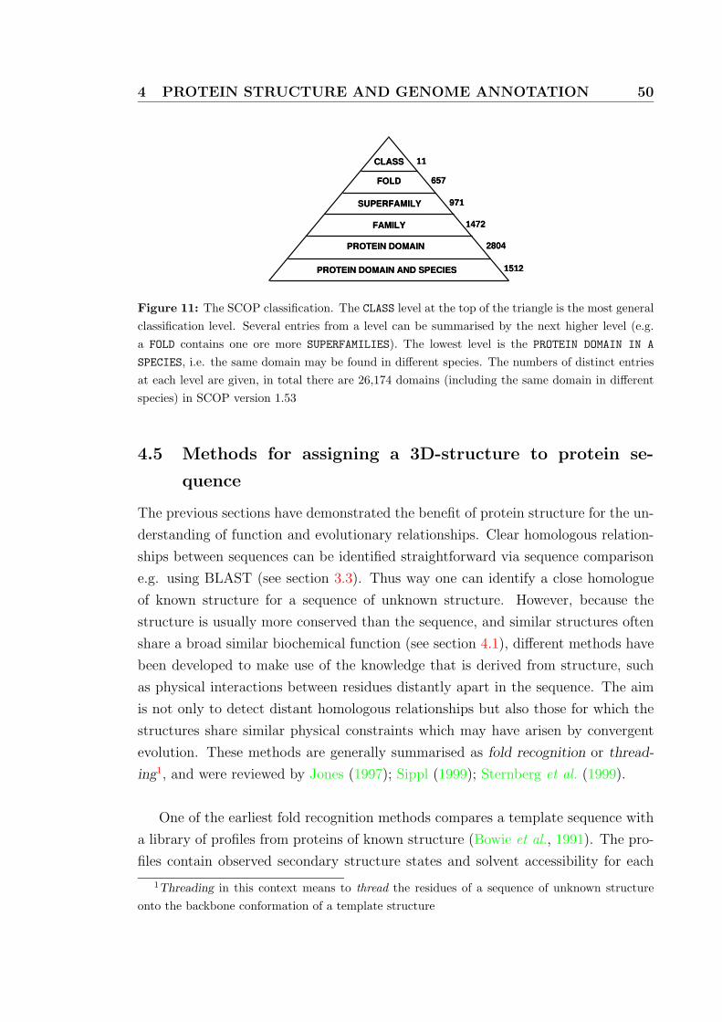
4 PROTEIN STRUCTURE AND GENOME ANNOTATION 50
CLASS
FOLD
SUPERFAMILY
FAMILY
PROTEIN DOMAIN
PROTEIN DOMAIN AND SPECIES
11
657
971
1472
2804
1512
Figure 11: The SCOP classification. The CLASS level at the top of the triangle is the most generalclassification level. Several entries from a level can be summarised by the next higher level (e.g.a FOLD contains one ore more SUPERFAMILIES). The lowest level is the PROTEIN DOMAIN IN A
SPECIES, i.e. the same domain may be found in different species. The numbers of distinct entriesat each level are given, in total there are 26,174 domains (including the same domain in differentspecies) in SCOP version 1.53
4.5 Methods for assigning a 3D-structure to protein se-
quence
The previous sections have demonstrated the benefit of protein structure for the un-
derstanding of function and evolutionary relationships. Clear homologous relation-
ships between sequences can be identified straightforward via sequence comparison
e.g. using BLAST (see section 3.3). Thus way one can identify a close homologue
of known structure for a sequence of unknown structure. However, because the
structure is usually more conserved than the sequence, and similar structures often
share a broad similar biochemical function (see section 4.1), different methods have
been developed to make use of the knowledge that is derived from structure, such
as physical interactions between residues distantly apart in the sequence. The aim
is not only to detect distant homologous relationships but also those for which the
structures share similar physical constraints which may have arisen by convergent
evolution. These methods are generally summarised as fold recognition or thread-
ing1, and were reviewed by Jones (1997); Sippl (1999); Sternberg et al. (1999).
One of the earliest fold recognition methods compares a template sequence with
a library of profiles from proteins of known structure (Bowie et al., 1991). The pro-
files contain observed secondary structure states and solvent accessibility for each
1Threading in this context means to thread the residues of a sequence of unknown structureonto the backbone conformation of a template structure
4 PROTEIN STRUCTURE AND GENOME ANNOTATION 51
residue position. A statistical analysis of all 20 amino acids with their states is
performed for all proteins of known structure, calculating a score for each amino
acid type in each state, which is used to score each residue of a target sequence in
the templates residues states.
One of the most successful methods developed was THREADER (Jones et al.,
1992) which uses pair-potentials to evaluate an energy function for the target residues
in a template structure. Pair-potentials introduced by Sippl (1990); Hendlich et al.
(1990) are derived by analysing the surrounding residues in a given radius in space
for a given residue. This is a measure for the preferred amino acid environment for
a given residue.
Advances in secondary structure predictions based on multiple sequence align-
ments and neural networks (Rost & Sander, 1993b,a; Jones, 1999) enhanced fold
recognition (similar 3D-structures have the a similar secondary structure content
and topologies) and were frequently incorporated into fold recognition methods.
In the 4th CASP competition (Critical Assessment of Structure Prediction) in
2000, a blind trial to predict the fold of structures that were held back temporar-
ily from publication for the purpose of CASP, the 3D-PSSM method performed
best under the fully automated methods (Kelley et al., 2000). Different methods
are combined to score the compatibility of a target sequence with each library se-
quence represented by a set of profiles that are derived from superimposed structures,
solvent-potentials, secondary structure prediction and sequence homology.
If more information than just the general fold is required and a homologue of
known structure is available, homology based modelling can be applied to build an
accurate structural model that includes sidechains. The assumption for homology
modelling is that the target sequence will have a similar fold, and therefore a similar
backbone conformation for the main secondary structure elements. The backbone
conformation of the homologue of known structure is used as a template onto which
the sidechains of the target are placed. The model may be refined using different
force fields (e.g. Sali & Blundell (1993); Sanchez & Sali (1997b)), see Sanchez &
Sali (1997a); Moult (1999) for a review on comparative modelling. Flexible loops
and gaps are difficult to model, and special methods have been developed to tackle
this problem (Bates et al., 1997). The quality of homology models strongly depends

4 PROTEIN STRUCTURE AND GENOME ANNOTATION 52
on the accuracy of the alignment between the target and the template. Reasonable
models that include sidechains and flexible loops require at least 30% sequence
identity (Sanchez & Sali, 1998; Bates et al., 1997; Fischer et al., 1999). Structural
genomics projects benefit from the conservation of protein structure by building
reliable models for closely related sequences (see section 4.3 on page 47). The growth
of the sequence database and the expected growth of the protein structure database
will increase the number of relationships with >30% sequence identity, increasing
template selection via straightforward sequence search methods such as BLAST.

REFERENCES 53
References
Acharya, K. R., D. I. Stuart, N. P. Walker, M. Lewis & D. C. Phillips (1989). Refined
structure of baboon alpha-lactalbumin at 1.7 A resolution. Comparison with C-type
lysozyme. J Mol Biol , 208(1):99–127.
Adams, M. D., S. E. Celniker, R. A. Holt, C. A. Evans, J. D. Gocayne et al. (2000). The
genome sequence of Drosophila melanogaster. Science, 287(5461):2185–2195.
Alm, R. A., L. S. Ling, D. T. Moir, B. L. King, E. D. Brown et al. (1999). Genomic-
sequence comparison of two unrelated isolates of the human gastric pathogen Helicobac-
ter pylori. Nature, 397(6715):176–180.
Aloy, P., E. Querol, F. X. Aviles & M. J. Sternberg (2001). Automated structure-based
prediction of functional sites in proteins: applications to assessing the validity of inher-
iting protein function from homology in genome annotation and to protein docking. J
Mol Biol , 311(2):395–408.
Altschul, S. F., R. Bundschuh, R. Olsen & T. Hwa (2001). The estimation of statistical
parameters for local alignment score distributions. Nucleic Acids Res, 29(2):351–361.
Altschul, S. F. & W. Gish (1996). Local alignment statistics. Methods Enzymol , 266:460–
480.
Altschul, S. F., W. Gish, W. Miller, E. W. Myers & D. J. Lipman (1990). Basic local
alignment search tool. J Mol Biol , 215(3):403–410.
Altschul, S. F. & E. V. Koonin (1998). Iterated profile searches with PSI-BLAST–a tool
for discovery in protein databases. Trends Biochem Sci , 23(11):444–447.
Altschul, S. F., T. L. Madden, A. A. Schaffer, J. Zhang, Z. Zhang et al. (1997). Gapped
BLAST and PSI-BLAST: a new generation of protein database search programs. Nucleic
Acids Res, 25(17):3389–3402.
Andersson, S. G., A. Zomorodipour, J. O. Andersson, T. Sicheritz-Ponten, U. C. Als-
mark et al. (1998). The genome sequence of Rickettsia prowazekii and the origin of
mitochondria. Nature, 396(6707):133–140.
Apic, G., J. Gough & S. A. Teichmann (2001). Domain combinations in archaeal, eubac-
terial and eukaryotic proteomes. J Mol Biol , 310(2):311–325.
Apweiler, R., T. K. Attwood, A. Bairoch, A. Bateman, E. Birney et al. (2001). The
InterPro database, an integrated documentation resource for protein families, domains
and functional sites. Nucleic Acids Res, 29(1):37–40.
REFERENCES 54
Aravind, L. & E. V. Koonin (1999). Gleaning non-trivial structural, functional and
evolutionary information about proteins by iterative database searches. J Mol Biol ,
287(5):1023–1040.
Ashburner, M., C. A. Ball, J. A. Blake, D. Botstein, H. Butler et al. (2000). Gene
ontology: tool for the unification of biology. The Gene Ontology Consortium. Nat
Genet , 25(1):25–29.
Attwood, T. K., M. J. Blythe, D. R. Flower, A. Gaulton, J. E. Mabey et al. (2002).
PRINTS and PRINTS-S shed light on protein ancestry. Nucleic Acids Res, 30(1):239–
241.
Bairoch, A. & R. Apweiler (2000). The SWISS-PROT protein sequence database and its
supplement TrEMBL in 2000. Nucleic Acids Res, 28(1):45–48.
Barker, W. C., J. S. Garavelli, H. Huang, P. B. McGarvey, B. C. Orcutt et al. (2000).
The protein information resource (PIR). Nucleic Acids Res, 28(1):41–44.
Bateman, A., E. Birney, L. Cerruti, R. Durbin, L. Etwiller et al. (2002). The Pfam protein
families database. Nucleic Acids Res, 30(1):276–280.
Bateman, A., E. Birney, R. Durbin, S. R. Eddy, R. D. Finn et al. (1999). Pfam 3.1: 1313
multiple alignments and profile HMMs match the majority of proteins. Nucleic Acids
Res, 27(1):260–262.
Bates, P. A., R. M. Jackson & M. J. Sternberg (1997). Model building by comparison: a
combination of expert knowledge and computer automation. Proteins, Suppl 1:59–67.
Bax, B., P. S. Carter, C. Lewis, A. R. Guy, A. Bridges et al. (2001). The structure of
phosphorylated GSK-3beta complexed with a peptide, FRATtide, that inhibits beta-
catenin phosphorylation. Structure, 9(12):1143–1152.
Bellman, R. (1957). Dynamic Programming . Princeton University Press, Princeton, New
Jersey, USA.
Benson, D. A., I. Karsch-Mizrachi, D. J. Lipman, J. Ostell, B. A. Rapp et al. (2002).
GenBank. Nucleic Acids Res, 30(1):17–20.
Berman, H. M., J. Westbrook, Z. Feng, G. Gilliland, T. N. Bhat et al. (2000). The Protein
Data Bank. Nucleic Acids Res, 28(1):235–242.
Bernal, A., U. Ear & N. Kyrpides (2001). Genomes OnLine Database (GOLD): a monitor
of genome projects world-wide. Nucleic Acids Res, 29(1):126–127.
REFERENCES 55
Blake, C. C., D. F. Koenig, G. A. Mair, A. C. North, D. C. Phillips et al. (1965). Struc-
ture of hen egg-white lysozyme. A three-dimensional Fourier synthesis at 2 Angstrom
resolution. Nature, 206(986):757–761.
Blattner, F. R., G. r. Plunkett, C. A. Bloch, N. T. Perna, V. Burland et al. (1997).
The complete genome sequence of Escherichia coli K-12. Science, 277(5331):1453–1474.
Comment.
Bolotin, A., P. Wincker, S. Mauger, O. Jaillon, K. Malarme et al. (2001). The complete
genome sequence of the lactic acid bacterium Lactococcus lactis ssp. lactis IL1403.
Genome Res, 11(5):731–753.
Bowie, J. U., R. Luthy & D. Eisenberg (1991). A method to identify protein sequences
that fold into a known three-dimensional structure. Science, 253(5016):164–170.
Bowman, S., D. Lawson, D. Basham, D. Brown, T. Chillingworth et al. (1999). The
complete nucleotide sequence of chromosome 3 of Plasmodium falciparum. Nature,
400(6744):532–538.
Brenner, S. E., D. Barken & M. Levitt (1999). The PRESAGE database for structural
genomics. Nucleic Acids Res, 27(1):251–253.
Brenner, S. E., C. Chothia & T. J. Hubbard (1997). Population statistics of protein
structures: lessons from structural classifications. Curr Opin Struct Biol , 7(3):369–376.
Bujacz, G., M. Jaskolski, J. Alexandratos, A. Wlodawer, G. Merkel et al. (1996). The cat-
alytic domain of avian sarcoma virus integrase: conformation of the active-site residues
in the presence of divalent cations. Structure, 4(1):89–96.
Bult, C. J., O. White, G. J. Olsen, L. Zhou, R. D. Fleischmann et al. (1996). Complete
genome sequence of the methanogenic archaeon, Methanococcus jannaschii. Science,
273(5278):1058–1073.
Burge, C. & S. Karlin (1997). Prediction of complete gene structures in human genomic
DNA. J Mol Biol , 268(1):78–94.
Burley, S. K. (2000). An overview of structural genomics. Nat Struct Biol , 7 Suppl:932–
934.
Chambaud, I., R. Heilig, S. Ferris, V. Barbe, D. Samson et al. (2001). The complete
genome sequence of the murine respiratory pathogen Mycoplasma pulmonis. Nucleic
Acids Res, 29(10):2145–2153.

REFERENCES 56
Chothia, C. & A. M. Lesk (1986). The relation between the divergence of sequence and
structure in proteins. EMBO J , 5(4):823–826.
Cole, S. T., R. Brosch, J. Parkhill, T. Garnier, C. Churcher et al. (1998). Deciphering the
biology of Mycobacterium tuberculosis from the complete genome sequence. Nature,
393(6685):537–544.
Cole, S. T., K. Eiglmeier, J. Parkhill, K. D. James, N. R. Thomson et al. (2001). Massive
gene decay in the leprosy bacillus. Nature, 409(6823):1007–1011.
Conte, L. L., S. E. Brenner, T. J. P. Hubbard, C. Chothia & A. G. Murzin (2002). SCOP
database in 2002: refinements accommodate structural genomics. Nucleic Acids Res,
30(1):264–267.
Corpet, F., F. Servant, J. Gouzy & D. Kahn (2000). ProDom and ProDom-CG: tools for
protein domain analysis and whole genome comparisons. Nucleic Acids Res, 28(1):267–
269.
Cross, D. A., D. R. Alessi, P. Cohen, M. Andjelkovich & B. A. Hemmings (1995). Inhi-
bition of glycogen synthase kinase-3 by insulin mediated by protein kinase B. Nature,
378(6559):785–789.
Dajani, R., E. Fraser, S. M. Roe, N. Young, V. Good et al. (2001). Crystal structure
of glycogen synthase kinase 3 beta: structural basis for phosphate-primed substrate
specificity and autoinhibition. Cell , 105(6):721–732.
Davies, J. F., Z. Hostomska, Z. Hostomsky, S. R. Jordan & D. A. Matthews (1991).
Crystal structure of the ribonuclease H domain of HIV-1 reverse transcriptase. Science,
252(5002):88–95.
Dayhoff, M. O., R. M. Schwartz & B. C. Orcutt (1978). Atlas of Protein Sequence and
Structure, volume 5 of 3 , pages 345–352. Natl. Biomed. Res. Found., Washington, DC.
Deckert, G., P. V. Warren, T. Gaasterland, W. G. Young, A. L. Lenox et al. (1998).
The complete genome of the hyperthermophilic bacterium Aquifex aeolicus. Nature,
392(6674):353–358.
Devos, D. & A. Valencia (2000). Practical limits of function prediction. Proteins,
41(1):98–107.
Diamond, R. (1974). Real-space refinement of the structure of hen egg-white lysozyme.
J Mol Biol , 82(3):371–391.
REFERENCES 57
Douglas, S., S. Zauner, M. Fraunholz, M. Beaton, S. Penny et al. (2001). The highly
reduced genome of an enslaved algal nucleus. Nature, 410(6832):1091–1096.
Dyda, F., A. B. Hickman, T. M. Jenkins, A. Engelman, R. Craigie et al. (1994). Crystal
structure of the catalytic domain of HIV-1 integrase: similarity to other polynucleotidyl
transferases. Science, 266(5193):1981–1986.
Eddy, S. R. (1998). Profile hidden Markov models. Bioinformatics, 14(9):755–763.
Falquet, L., M. Pagni, P. Bucher, N. Hulo, C. J. A. Sigrist et al. (2002). The PROSITE
database, its status in 2002. Nucleic Acids Res, 30(1):235–238.
Ferretti, J. J., W. M. McShan, D. Ajdic, D. J. Savic, G. Savic et al. (2001). Complete
genome sequence of an M1 strain of Streptococcus pyogenes. Proc Natl Acad Sci U S
A, 98(8):4658–4663.
Fiol, C. J., J. S. Williams, C. H. Chou, Q. M. Wang, P. J. Roach et al. (1994). A secondary
phosphorylation of CREB341 at Ser129 is required for the cAMP-mediated control of
gene expression. A role for glycogen synthase kinase-3 in the control of gene expression.
J Biol Chem, 269(51):32187–32193.
Fischer, D., C. Barret, K. Bryson, A. Elofsson, A. Godzik et al. (1999). CAFASP-1:
critical assessment of fully automated structure prediction methods. Proteins, Suppl
3:209–217.
Fleischmann, R. D., M. D. Adams, O. White, R. A. Clayton, E. F. Kirkness et al. (1995).
Whole-genome random sequencing and assembly of Haemophilus influenzae Rd. Sci-
ence, 269(5223):496–512.
Fraser, C. M., S. Casjens, W. M. Huang, G. G. Sutton, R. Clayton et al. (1997). Genomic
sequence of a Lyme disease spirochaete, Borrelia burgdorferi. Nature, 390(6660):580–
586.
Fraser, C. M., J. D. Gocayne, O. White, M. D. Adams, R. A. Clayton et al. (1995). The
minimal gene complement of Mycoplasma genitalium. Science, 270(5235):397–403.
Fraser, C. M., S. J. Norris, G. M. Weinstock, O. White, G. G. Sutton et al. (1998).
Complete genome sequence of Treponema pallidum, the syphilis spirochete. Science,
281(5375):375–388.
Galibert, F., T. M. Finan, S. R. Long, A. Puhler, P. Abola et al. (2001). The composite
genome of the legume symbiont Sinorhizobium meliloti. Science, 293(5530):668–672.

REFERENCES 58
Gardner, M. J., H. Tettelin, D. J. Carucci, L. M. Cummings, L. Aravind et al. (1998).
Chromosome 2 sequence of the human malaria parasite Plasmodium falciparum. Sci-
ence, 282(5391):1126–1132.
Glaser, P., L. Frangeul, C. Buchrieser, C. Rusniok, A. Amend et al. (2001). Comparative
genomics of Listeria species. Science, 294(5543):849–852.
Glass, J. I., E. J. Lefkowitz, J. S. Glass, C. R. Heiner, E. Y. Chen et al. (2000).
The complete sequence of the mucosal pathogen Ureaplasma urealyticum. Nature,
407(6805):757–762.
Gough, J. & C. Chothia (2002). SUPERFAMILY: HMMs representing all proteins of
known structure. SCOP sequence searches, alignments and genome assignments. Nucleic
Acids Res, 30(1):268–272.
Govindarajan, S., R. Recabarren & R. A. Goldstein (1999). Estimating the total number
of protein folds. Proteins, 35(4):408–414.
Gracy, J. & P. Argos (1998). DOMO: a new database of aligned protein domains. Trends
Biochem Sci , 23(12):495–497.
Gribskov, M., A. D. McLachlan & D. Eisenberg (1987). Profile analysis: detection of
distantly related proteins. Proc Natl Acad Sci U S A, 84(13):4355–4358.
Hayashi, T., K. Makino, M. Ohnishi, K. Kurokawa, K. Ishii et al. (2001). Complete ge-
nome sequence of enterohemorrhagic Escherichia coli O157:H7 and genomic comparison
with a laboratory strain K-12. DNA Res, 8(1):11–22.
Hegyi, H. & M. Gerstein (1999). The relationship between protein structure and function:
a comprehensive survey with application to the yeast genome. J Mol Biol , 288(1):147–
164.
Hegyi, H. & M. Gerstein (2001). Annotation transfer for genomics: measuring functional
divergence in multi-domain proteins. Genome Res, 11(10):1632–1640.
Heidelberg, J. F., J. A. Eisen, W. C. Nelson, R. A. Clayton, M. L. Gwinn et al. (2000).
DNA sequence of both chromosomes of the cholera pathogen Vibrio cholerae. Nature,
406(6795):477–483.
Hendlich, M., P. Lackner, S. Weitckus, H. Floeckner, R. Froschauer et al. (1990). Iden-
tification of native protein folds amongst a large number of incorrect models. The
calculation of low energy conformations from potentials of mean force. J Mol Biol ,
216(1):167–180.
REFERENCES 59
Henikoff, J. G., E. A. Greene, S. Pietrokovski & S. Henikoff (2000). Increased coverage
of protein families with the blocks database servers. Nucleic Acids Res, 28(1):228–230.
Henikoff, S. & J. G. Henikoff (1992). Amino acid substitution matrices from protein
blocks. Proc Natl Acad Sci U S A, 89(22):10915–10919.
Henikoff, S. & J. G. Henikoff (1993). Performance evaluation of amino acid substitution
matrices. Proteins, 17(1):49–61.
Henikoff, S., J. G. Henikoff, W. J. Alford & S. Pietrokovski (1995). Automated con-
struction and graphical presentation of protein blocks from unaligned sequences. Gene,
163(2):GC17–26.
Henikoff, S., J. G. Henikoff & S. Pietrokovski (1999). Blocks+: a non-redundant data-
base of protein alignment blocks derived from multiple compilations. Bioinformatics,
15(6):471–479.
Himmelreich, R., H. Hilbert, H. Plagens, E. Pirkl, B. C. Li et al. (1996). Complete
sequence analysis of the genome of the bacterium Mycoplasma pneumoniae. Nucleic
Acids Res, 24(22):4420–4449.
Holm, L. & C. Sander (1997). An evolutionary treasure: unification of a broad set of
amidohydrolases related to urease. Proteins, 28(1):72–82.
Hoskins, J., W. E. J. Alborn, J. Arnold, L. C. Blaszczak, S. Burgett et al. (2001). Genome
of the bacterium Streptococcus pneumoniae strain R6. J Bacteriol , 183(19):5709–5717.
Hubbard, T., D. Barker, E. Birney, G. Cameron, Y. Chen et al. (2002). The Ensembl
genome database project. Nucleic Acids Res, 30(1):38–41.
Jolles, P., F. Schoentgen, J. Jolles, D. E. Dobson, E. M. Prager et al. (1984). Stomach
lysozymes of ruminants. II. Amino acid sequence of cow lysozyme 2 and immunological
comparisons with other lysozymes. J Biol Chem, 259(18):11617–11625.
Jonassen, I., I. Eidhammer & W. R. Taylor (1999). Discovery of local packing motifs in
protein structures. Proteins, 34(2):206–219.
Jones, D. T. (1997). Progress in protein structure prediction. Curr Opin Struct Biol ,
7(3):377–387.
Jones, D. T. (1999). Protein secondary structure prediction based on position-specific
scoring matrices. J Mol Biol , 292(2):195–202.
REFERENCES 60
Jones, D. T., W. R. Taylor & J. M. Thornton (1992). A new approach to protein fold
recognition. Nature, 358(6381):86–89.
Kalman, S., W. Mitchell, R. Marathe, C. Lammel, J. Fan et al. (1999). Comparative
genomes of Chlamydia pneumoniae and C. trachomatis. Nat Genet , 21(4):385–389.
Kanehisa, M., S. Goto, S. Kawashima & A. Nakaya (2002). The KEGG databases at
GenomeNet. Nucleic Acids Res, 30(1):42–46.
Kaneko, T., Y. Nakamura, S. Sato, E. Asamizu, T. Kato et al. (2000). Complete genome
structure of the nitrogen-fixing symbiotic bacterium Mesorhizobium loti. DNA Res,
7(6):331–338.
Kaneko, T., S. Sato, H. Kotani, A. Tanaka, E. Asamizu et al. (1996). Sequence analysis
of the genome of the unicellular cyanobacterium Synechocystis sp. strain PCC6803. II.
Sequence determination of the entire genome and assignment of potential protein-coding
regions. DNA Res, 3(3):109–136.
Karlin, S. & S. F. Altschul (1990). Methods for assessing the statistical significance of
molecular sequence features by using general scoring schemes. Proc Natl Acad Sci U S
A, 87(6):2264–2268.
Karlin, S. & S. F. Altschul (1993). Applications and statistics for multiple high-scoring
segments in molecular sequences. Proc Natl Acad Sci U S A, 90(12):5873–5877.
Karp, P. D., M. Riley, M. Saier, I. T. Paulsen, J. Collado-Vides et al. (2002). The EcoCyc
Database. Nucleic Acids Res, 30(1):56–58.
Karplus, K., C. Barrett & R. Hughey (1998). Hidden Markov models for detecting remote
protein homologies. Bioinformatics, 14(10):846–856.
Katayanagi, K., M. Miyagawa, M. Matsushima, M. Ishikawa, S. Kanaya et al. (1990).
Three-dimensional structure of ribonuclease H from E. coli. Nature, 347(6290):306–
309.
Katayanagi, K., M. Okumura & K. Morikawa (1993). Crystal structure of Escherichia coli
RNase HI in complex with Mg2+ at 2.8 A resolution: proof for a single Mg(2+)-binding
site. Proteins, 17(4):337–346.
Kawarabayasi, Y., Y. Hino, H. Horikawa, K. Jin-no, M. Takahashi et al. (2001). Com-
plete genome sequence of an aerobic thermoacidophilic crenarchaeon, Sulfolobus toko-
daii strain7. DNA Res, 8(4):123–140.
REFERENCES 61
Kawarabayasi, Y., Y. Hino, H. Horikawa, S. Yamazaki, Y. Haikawa et al. (1999). Complete
genome sequence of an aerobic hyper-thermophilic crenarchaeon, Aeropyrum pernix K1.
DNA Res, 6(2):83–101, 145–52.
Kawarabayasi, Y., M. Sawada, H. Horikawa, Y. Haikawa, Y. Hino et al. (1998). Complete
sequence and gene organization of the genome of a hyper-thermophilic archaebacterium,
Pyrococcus horikoshii OT3. DNA Res, 5(2):55–76.
Kawashima, T., N. Amano, H. Koike, S. Makino, S. Higuchi et al. (2000). Archaeal
adaptation to higher temperatures revealed by genomic sequence of Thermoplasma vol-
canium. Proc Natl Acad Sci U S A, 97(26):14257–14262.
Kelley, L. A., R. M. MacCallum & M. J. Sternberg (2000). Enhanced genome annotation
using structural profiles in the program 3D-PSSM. J Mol Biol , 299(2):499–520.
Klenk, H. P., R. A. Clayton, J. F. Tomb, O. White, K. E. Nelson et al. (1997). The
complete genome sequence of the hyperthermophilic, sulphate-reducing archaeon Ar-
chaeoglobus fulgidus. Nature, 390(6658):364–370.
Krogh, A., M. Brown, I. S. Mian, K. Sjolander & D. Haussler (1994). Hidden Markov mod-
els in computational biology. Applications to protein modeling. J Mol Biol , 235(5):1501–
1531.
Krogh, A., B. Larsson, G. von Heijne & E. L. Sonnhammer (2001). Predicting transmem-
brane protein topology with a hidden Markov model: application to complete genomes.
J Mol Biol , 305(3):567–580.
Kulkosky, J., K. S. Jones, R. A. Katz, J. P. Mack & A. M. Skalka (1992). Residues critical
for retroviral integrative recombination in a region that is highly conserved among
retroviral/retrotransposon integrases and bacterial insertion sequence transposases. Mol
Cell Biol , 12(5):2331–2338.
Kunst, F., N. Ogasawara, I. Moszer, A. M. Albertini, G. Alloni et al. (1997). The
complete genome sequence of the gram-positive bacterium Bacillus subtilis. Nature,
390(6657):249–256.
Kuroda, M., T. Ohta, I. Uchiyama, T. Baba, H. Yuzawa et al. (2001). Whole genome
sequencing of meticillin-resistant Staphylococcus aureus. Lancet , 357(9264):1225–1240.
Lander, E. S., L. M. Linton, B. Birren, C. Nusbaum, M. C. Zody et al. (2001). Initial
sequencing and analysis of the human genome. Nature, 409(6822):860–921.
REFERENCES 62
Letunic, I., L. Goodstadt, N. J. Dickens, T. Doerks, J. Schultz et al. (2002). Recent
improvements to the SMART domain-based sequence annotation resource. Nucleic
Acids Res, 30(1):242–244.
Lewis, S., M. Ashburner & M. G. Reese (2000). Annotating eukaryote genomes. Curr
Opin Struct Biol , 10(3):349–354.
Marchler-Bauer, A., A. R. Panchenko, B. A. Shoemaker, P. A. Thiessen, L. Y. Geer et al.
(2002). CDD: a database of conserved domain alignments with links to domain three-
dimensional structure. Nucleic Acids Res, 30(1):281–283.
Martin, A. C., C. A. Orengo, E. G. Hutchinson, S. Jones, M. Karmirantzou et al. (1998).
Protein folds and functions. Structure, 6(7):875–884.
May, B. J., Q. Zhang, L. L. Li, M. L. Paustian, T. S. Whittam et al. (2001). Com-
plete genomic sequence of Pasteurella multocida, Pm70. Proc Natl Acad Sci U S A,
98(6):3460–3465.
McClelland, M., K. E. Sanderson, J. Spieth, S. W. Clifton, P. Latreille et al. (2001).
Complete genome sequence of Salmonella enterica serovar Typhimurium LT2. Nature,
413(6858):852–856.
McKenzie, H. A. (1996). alpha-Lactalbumins and lysozymes. EXS , 75:365–409.
McKenzie, H. A. & F. H. J. White (1991). Lysozyme and alpha-lactalbumin: structure,
function, and interrelationships. Adv Protein Chem, 41:173–315.
Mott, R. (2000). Accurate formula for P-values of gapped local sequence and profile
alignments. J Mol Biol , 300(3):649–659.
Moult, J. (1999). Predicting protein three-dimensional structure. Curr Opin Biotechnol ,
10(6):583–588.
Murzin, A. G., S. E. Brenner, T. Hubbard & C. Chothia (1995). SCOP: a structural
classification of proteins database for the investigation of sequences and structures. J
Mol Biol , 247(4):536–540.
Myler, P. J., L. Audleman, T. deVos, G. Hixson, P. Kiser et al. (1999). Leishmania major
Friedlin chromosome 1 has an unusual distribution of protein-coding genes. Proc Natl
Acad Sci U S A, 96(6):2902–2906.
Needleman, S. B. & C. D. Wunsch (1970). A general method applicable to the search for
similarities in the amino acid sequence of two proteins. J Mol Biol , 48(3):443–453.

REFERENCES 63
Nelson, K. E., R. A. Clayton, S. R. Gill, M. L. Gwinn, R. J. Dodson et al. (1999).
Evidence for lateral gene transfer between Archaea and bacteria from genome sequence
of Thermotoga maritima. Nature, 399(6734):323–329.
Ng, W. V., S. P. Kennedy, G. G. Mahairas, B. Berquist, M. Pan et al. (2000). Genome
sequence of Halobacterium species NRC-1. Proc Natl Acad Sci U S A, 97(22):12176–
12181.
Nierman, W. C., T. V. Feldblyum, M. T. Laub, I. T. Paulsen, K. E. Nelson et al. (2001).
Complete genome sequence of Caulobacter crescentus. Proc Natl Acad Sci U S A,
98(7):4136–4141.
Nitta, K. (2002). Alpha-lactalbumin and (calcium-binding) lysozyme. Methods Mol Biol ,
172:211–224.
Nitta, K., H. Tsuge, K. Shimazaki & S. Sugai (1988). Calcium-binding lysozymes. Biol
Chem Hoppe Seyler , 369(8):671–675.
No authors listed (1997). The yeast genome directory. Nature, 387(6632 Suppl). Directory.
Nolling, J., G. Breton, M. V. Omelchenko, K. S. Makarova, Q. Zeng et al. (2001). Genome
sequence and comparative analysis of the solvent-producing bacterium Clostridium ace-
tobutylicum. J Bacteriol , 183(16):4823–4838.
Ogata, H., S. Audic, P. Renesto-Audiffren, P. E. Fournier, V. Barbe et al. (2001). Mech-
anisms of evolution in Rickettsia conorii and R. prowazekii. Science, 293(5537):2093–
2098.
Orengo, C. A., A. D. Michie, S. Jones, D. T. Jones, M. B. Swindells et al. (1997). CATH–a
hierarchic classification of protein domain structures. Structure, 5(8):1093–1108.
Orengo, C. A., A. E. Todd & J. M. Thornton (1999). From protein structure to function.
Curr Opin Struct Biol , 9(3):374–382.
Park, J., K. Karplus, C. Barrett, R. Hughey, D. Haussler et al. (1998). Sequence com-
parisons using multiple sequences detect three times as many remote homologues as
pairwise methods. J Mol Biol , 284(4):1201–1210.
Parkhill, J., M. Achtman, K. D. James, S. D. Bentley, C. Churcher et al. (2000a). Com-
plete DNA sequence of a serogroup A strain of Neisseria meningitidis Z2491. Nature,
404(6777):502–506.
REFERENCES 64
Parkhill, J., G. Dougan, K. D. James, N. R. Thomson, D. Pickard et al. (2001a). Complete
genome sequence of a multiple drug resistant Salmonella enterica serovar Typhi CT18.
Nature, 413(6858):848–852.
Parkhill, J., B. W. Wren, K. Mungall, J. M. Ketley, C. Churcher et al. (2000b). The ge-
nome sequence of the food-borne pathogen Campylobacter jejuni reveals hypervariable
sequences. Nature, 403(6770):665–668.
Parkhill, J., B. W. Wren, N. R. Thomson, R. W. Titball, M. T. Holden et al. (2001b). Ge-
nome sequence of Yersinia pestis, the causative agent of plague. Nature, 413(6855):523–
527.
Patthy, L. (1987). Detecting homology of distantly related proteins with consensus se-
quences. J Mol Biol , 198(4):567–577.
Pearl, F. M., N. Martin, J. E. Bray, D. W. Buchan, A. P. Harrison et al. (2001). A rapid
classification protocol for the CATH Domain Database to support structural genomics.
Nucleic Acids Res, 29(1):223–227.
Pearson, H. (2001). Biology’s name game. Nature, 411(6838):631–632.
Pearson, W. R. (1990). Rapid and sensitive sequence comparison with FASTP and
FASTA. Methods Enzymol , 183:63–98.
Pearson, W. R. & D. J. Lipman (1988). Improved tools for biological sequence comparison.
Proc Natl Acad Sci U S A, 85(8):2444–2448.
Perna, N. T., G. r. Plunkett, V. Burland, B. Mau, J. D. Glasner et al. (2001). Genome
sequence of enterohaemorrhagic Escherichia coli O157:H7. Nature, 409(6819):529–533.
Prager, E. M. & A. C. Wilson (1988). Ancient origin of lactalbumin from lysozyme:
analysis of DNA and amino acid sequences. J Mol Evol , 27(4):326–335.
Qian, J., N. M. Luscombe & M. Gerstein (2001). Protein family and fold occurrence in
genomes: power-law behaviour and evolutionary model. J Mol Biol , 313(4):673–681.
Read, T. D., R. C. Brunham, C. Shen, S. R. Gill, J. F. Heidelberg et al. (2000). Genome
sequences of Chlamydia trachomatis MoPn and Chlamydia pneumoniae AR39. Nucleic
Acids Res, 28(6):1397–1406.
Reese, M. G., G. Hartzell, N. L. Harris, U. Ohler, J. F. Abril et al. (2000). Genome
annotation assessment in Drosophila melanogaster. Genome Res, 10(4):483–501.

REFERENCES 65
Roberts, L. (1991). GRAIL seeks out genes buried in DNA sequence. Science,
254(5033):805. News.
Robinson, A. B. & L. R. Robinson (1991). Distribution of glutamine and asparagine
residues and their near neighbors in peptides and proteins. Proc Natl Acad Sci U S A,
88(20):8880–8884.
Rost, B. & C. Sander (1993a). Improved prediction of protein secondary structure by use
of sequence profiles and neural networks. Proc Natl Acad Sci U S A, 90(16):7558–7562.
Rost, B. & C. Sander (1993b). Prediction of protein secondary structure at better than
70accuracy. J Mol Biol , 232(2):584–599.
Rubin, G. M., M. D. Yandell, J. R. Wortman, G. L. Gabor Miklos., C. R. Nelson et al.
(2000). Comparative genomics of the eukaryotes. Science, 287(5461):2204–2215.
Ruepp, A., W. Graml, M. L. Santos-Martinez, K. K. Koretke, C. Volker et al. (2000).
The genome sequence of the thermoacidophilic scavenger Thermoplasma acidophilum.
Nature, 407(6803):508–513.
Russell, R. B. (1998). Detection of protein three-dimensional side-chain patterns: new
examples of convergent evolution. J Mol Biol , 279(5):1211–1227.
Russell, R. B., M. A. Saqi, P. A. Bates, R. A. Sayle & M. J. Sternberg (1998). Recognition
of analogous and homologous protein folds–assessment of prediction success and associ-
ated alignment accuracy using empirical substitution matrices. Protein Eng , 11(1):1–9.
Sali, A. & T. L. Blundell (1993). Comparative protein modelling by satisfaction of spatial
restraints. J Mol Biol , 234(3):779–815.
Sanchez, R., U. Pieper, F. Melo, N. Eswar, M. A. Marti-Renom et al. (2000). Protein
structure modeling for structural genomics. Nat Struct Biol , 7 Suppl:986–990.
Sanchez, R. & A. Sali (1997a). Advances in comparative protein-structure modelling.
Curr Opin Struct Biol , 7(2):206–214.
Sanchez, R. & A. Sali (1997b). Evaluation of comparative protein structure modeling by
MODELLER-3. Proteins, Suppl 1:50–58.
Sanchez, R. & A. Sali (1998). Large-scale protein structure modeling of the Saccharomyces
cerevisiae genome. Proc Natl Acad Sci U S A, 95(23):13597–13602.

REFERENCES 66
Schaffer, A. A., L. Aravind, T. L. Madden, S. Shavirin, J. L. Spouge et al. (2001).
Improving the accuracy of PSI-BLAST protein database searches with composition-
based statistics and other refinements. Nucleic Acids Res, 29(14):2994–3005.
Schaffer, A. A., Y. I. Wolf, C. P. Ponting, E. V. Koonin, L. Aravind et al. (1999). IMPALA:
matching a protein sequence against a collection of PSI-BLAST-constructed position-
specific score matrices. Bioinformatics, 15(12):1000–1011.
She, Q., R. K. Singh, F. Confalonieri, Y. Zivanovic, G. Allard et al. (2001). The complete
genome of the crenarchaeon Sulfolobus solfataricus P2. Proc Natl Acad Sci U S A,
98(14):7835–7840.
Shewale, J. G., S. K. Sinha & K. Brew (1984). Evolution of alpha-lactalbumins. The
complete amino acid sequence of the alpha-lactalbumin from a marsupial (Macropus ru-
fogriseus) and corrections to regions of sequence in bovine and goat alpha-lactalbumins.
J Biol Chem, 259(8):4947–4956.
Shigenobu, S., H. Watanabe, M. Hattori, Y. Sakaki & H. Ishikawa (2000). Genome
sequence of the endocellular bacterial symbiont of aphids Buchnera sp. APS. Nature,
407(6800):81–86.
Shirai, M., H. Hirakawa, M. Kimoto, M. Tabuchi, F. Kishi et al. (2000). Comparison
of whole genome sequences of Chlamydia pneumoniae J138 from Japan and CWL029
from USA. Nucleic Acids Res, 28(12):2311–2314.
Simpson, A. J., F. C. Reinach, P. Arruda, F. A. Abreu, M. Acencio et al. (2000).
The genome sequence of the plant pathogen Xylella fastidiosa. The Xylella fastid-
iosa Consortium of the Organization for Nucleotide Sequencing and Analysis. Nature,
406(6792):151–157.
Sippl, M. J. (1990). Calculation of conformational ensembles from potentials of mean
force. An approach to the knowledge-based prediction of local structures in globular
proteins. J Mol Biol , 213(4):859–883.
Sippl, M. J. (1999). An attempt to analyse progress in fold recognition from CASP1 to
CASP3. Proteins, 37(S3):226–230.
Skovgaard, M., L. J. Jensen, S. Brunak, D. Ussery & A. Krogh (2001). On the total
number of genes and their length distribution in complete microbial genomes. Trends
Genet , 17(8):425–428.

REFERENCES 67
Smith, D. R., L. A. Doucette-Stamm, C. Deloughery, H. Lee, J. Dubois et al. (1997).
Complete genome sequence of Methanobacterium thermoautotrophicum deltaH: func-
tional analysis and comparative genomics. J Bacteriol , 179(22):7135–7155.
Smith, S. G., M. Lewis, R. Aschaffenburg, R. E. Fenna, I. A. Wilson et al. (1987). Crys-
tallographic analysis of the three-dimensional structure of baboon alpha-lactalbumin at
low resolution. Homology with lysozyme. Biochem J , 242(2):353–360.
Smith, T. F. & M. S. Waterman (1981). Identification of common molecular subsequences.
J Mol Biol , 147(1):195–197.
Sonnhammer, E. L. & D. Kahn (1994). Modular arrangement of proteins as inferred from
analysis of homology. Protein Sci , 3(3):482–492.
Sonnhammer, E. L., G. von Heijne & A. Krogh (1998). A hidden Markov model for
predicting transmembrane helices in protein sequences. Proc Int Conf Intell Syst Mol
Biol , 6:175–182.
Stein, L. (2001). Genome annotation: from sequence to biology. Nat Rev Genet , 2(7):493–
503.
Stephens, R. S., S. Kalman, C. Lammel, J. Fan, R. Marathe et al. (1998). Genome
sequence of an obligate intracellular pathogen of humans: Chlamydia trachomatis. Sci-
ence, 282(5389):754–759.
Sternberg, M. J., P. A. Bates, L. A. Kelley & R. M. MacCallum (1999). Progress in
protein structure prediction: assessment of CASP3. Curr Opin Struct Biol , 9(3):368–
373. Congresses.
Stoesser, G., W. Baker, A. van Den. Broek., E. Camon, M. Garcia-Pastor et al. (2002).
The EMBL Nucleotide Sequence Database. Nucleic Acids Res, 30(1):21–26.
Stover, C. K., X. Q. Pham, A. L. Erwin, S. D. Mizoguchi, P. Warrener et al. (2000). Com-
plete genome sequence of Pseudomonas aeruginosa PA01, an opportunistic pathogen.
Nature, 406(6799):959–964.
Takami, H. & K. Horikoshi (2000). Analysis of the genome of an alkaliphilic Bacillus
strain from an industrial point of view. Extremophiles, 4(2):99–108.
Tatusov, R. L., S. F. Altschul & E. V. Koonin (1994). Detection of conserved segments
in proteins: iterative scanning of sequence databases with alignment blocks. Proc Natl
Acad Sci U S A, 91(25):12091–12095.

REFERENCES 68
Tatusov, R. L., E. V. Koonin & D. J. Lipman (1997). A genomic perspective on protein
families. Science, 278(5338):631–637.
Tatusov, R. L., D. A. Natale, I. V. Garkavtsev, T. A. Tatusova, U. T. Shankavaram et al.
(2001). The COG database: new developments in phylogenetic classification of proteins
from complete genomes. Nucleic Acids Res, 29(1):22–28.
Taylor, W. R. (1986). Identification of protein sequence homology by consensus template
alignment. J Mol Biol , 188(2):233–258.
Tettelin, H., K. E. Nelson, I. T. Paulsen, J. A. Eisen, T. D. Read et al. (2001). Com-
plete genome sequence of a virulent isolate of Streptococcus pneumoniae. Science,
293(5529):498–506.
Tettelin, H., N. J. Saunders, J. Heidelberg, A. C. Jeffries, K. E. Nelson et al. (2000).
Complete genome sequence of Neisseria meningitidis serogroup B strain MC58. Science,
287(5459):1809–1815.
The Arabidopsis Genome Initiative (2000). Analysis of the genome sequence of the flow-
ering plant Arabidopsis thaliana. Nature, 408(6814):796–815.
The C. elegans Sequencing Consortium (1998). Genome sequence of the nematode C.
elegans: a platform for investigating biology. Science, 282(5396):2012–2018.
The Gene Ontology Consortium (2001). Creating the gene ontology resource: design and
implementation. Genome Res, 11(8):1425–1433.
Thornton, J. M., C. A. Orengo, A. E. Todd & F. M. Pearl (1999). Protein folds, functions
and evolution. J Mol Biol , 293(2):333–342.
Thornton, J. M., A. E. Todd, D. Milburn, N. Borkakoti & C. A. Orengo (2000). From
structure to function: approaches and limitations. Nat Struct Biol , 7 Suppl:991–994.
Todd, A. E., C. A. Orengo & J. M. Thornton (2001). Evolution of function in protein
superfamilies, from a structural perspective. J Mol Biol , 307(4):1113–1143.
Tomb, J. F., O. White, A. R. Kerlavage, R. A. Clayton, G. G. Sutton et al. (1997).
The complete genome sequence of the gastric pathogen Helicobacter pylori. Nature,
388(6642):539–547.
Tusnady, G. E. & I. Simon (2001). The HMMTOP transmembrane topology prediction
server. Bioinformatics, 17(9):849–850.

REFERENCES 69
Uberbacher, E. C. & R. J. Mural (1991). Locating protein-coding regions in human DNA
sequences by a multiple sensor-neural network approach. Proc Natl Acad Sci U S A,
88(24):11261–11265.
Ursing, B. M., F. H. J. van Enckevort, J. A. M. Leunissen & R. J. Siezen (2002). EXProt:
a database for proteins with an experimentally verified function. Nucleic Acids Res,
30(1):50–51.
Venter, J. C., M. D. Adams, E. W. Myers, P. W. Li, R. J. Mural et al. (2001). The
sequence of the human genome. Science, 291(5507):1304–1351.
Vitkup, D., E. Melamud, J. Moult & C. Sander (2001). Completeness in structural
genomics. Nat Struct Biol , 8(6):559–566.
Wallace, A. C., N. Borkakoti & J. M. Thornton (1997). TESS: a geometric hashing
algorithm for deriving 3D coordinate templates for searching structural databases. Ap-
plication to enzyme active sites. Protein Sci , 6(11):2308–2323.
Waterman, M. S. & M. Vingron (1994). Rapid and accurate estimates of statistical
significance for sequence data base searches. Proc Natl Acad Sci U S A, 91(11):4625–
4628.
White, O., J. A. Eisen, J. F. Heidelberg, E. K. Hickey, J. D. Peterson et al. (1999).
Genome sequence of the radioresistant bacterium Deinococcus radiodurans R1. Science,
286(5444):1571–1577.
Wilbur, W. J. & D. J. Lipman (1983). Rapid similarity searches of nucleic acid and
protein data banks. Proc Natl Acad Sci U S A, 80(3):726–730.
Wilson, C. A., J. Kreychman & M. Gerstein (2000). Assessing annotation transfer for
genomics: quantifying the relations between protein sequence, structure and function
through traditional and probabilistic scores. J Mol Biol , 297(1):233–249.
Wolf, Y. I., N. V. Grishin & E. V. Koonin (2000). Estimating the number of protein folds
and families from complete genome data. J Mol Biol , 299(4):897–905.
Wood, D. W., J. C. Setubal, R. Kaul, D. E. Monks, J. P. Kitajima et al. (2001).
The genome of the natural genetic engineer Agrobacterium tumefaciens C58. Science,
294(5550):2317–2323.
Wood, T. C. & W. R. Pearson (1999). Evolution of protein sequences and structures. J
Mol Biol , 291(4):977–995.

REFERENCES 70
Wootton, J. C. (1994). Non-globular domains in protein sequences: automated segmen-
tation using complexity measures. Comput Chem, 18(3):269–285.
Xu, Y., J. R. Einstein, R. J. Mural, M. Shah & E. C. Uberbacher (1994). An improved
system for exon recognition and gene modeling in human DNA sequences. Proc Int
Conf Intell Syst Mol Biol , 2:376–384.
Yang, W. & T. A. Steitz (1995). Recombining the structures of HIV integrase, RuvC and
RNase H. Structure, 3(2):131–134.
Yi, T. M. & E. S. Lander (1994). Recognition of related proteins by iterative template
refinement (ITR). Protein Sci , 3(8):1315–1328.
Zdobnov, E. M. & R. Apweiler (2001). InterProScan–an integration platform for the
signature-recognition methods in InterPro. Bioinformatics, 17(9):847–848.
Zhang, C. & C. DeLisi (1998). Estimating the number of protein folds. J Mol Biol ,
284(5):1301–1305.
Zhang, J., F. Zhang, D. Ebert, M. H. Cobb & E. J. Goldsmith (1995). Activity of the
MAP kinase ERK2 is controlled by a flexible surface loop. Structure, 3(3):299–307.