an introduction to applicable game theory - home |...

Journal of Economic Perspectives—Volume 11, Number 1—Winter 1997—Pages 127–149

An Introduction to Applicable GameTheory

Robert Gibbons

G ame theory is rampant in economics. Having long ago invaded industrialorganization, game-theoretic modeling is now commonplace in interna-tional, labor, macro and public finance, and it is gathering steam in de-

velopment and economic history. Nor is economics alone: accounting, finance, law,marketing, political science and sociology are beginning similar experiences. Manymodelers use game theory because it allows them to think like an economist whenprice theory does not apply. That is, game-theoretic models allow economists tostudy the implications of rationality, self-interest and equilibrium, both in marketinteractions that are modeled as games (such as where small numbers, hiddeninformation, hidden actions or incomplete contracts are present) and in nonmar-ket interactions (such as between a regulator and a firm, a boss and a worker, andso on).

Many applied economists seem to appreciate that game theory can comple-ment price theory in this way, but nonetheless find game theory more an entrybarrier than a useful tool. This paper is addressed to such readers. I try to give cleardefinitions and intuitive examples of the basic kinds of games and the basic solutionconcepts. Perhaps more importantly, I try to distill the welter of solution conceptsand other jargon into a few basic principles that permeate the literature. Thus, Ienvision this paper as a tutorial for economists who have brushed up against gametheory but have not (yet) read a book on the subject.

The theory is presented in four sections, corresponding to whether the game

/ av1 3006 0002 Mp 127 Friday Oct 27 12:23 PM LP–JEP 00023007

in question is static or dynamic and to whether it has complete or incomplete

� Robert Gibbons is the Charles Dyson Professor of Economics and Organizations, JohnsonGraduate School of Management, Cornell University, Ithaca, New York, and Research Asso-ciate, National Bureau of Economic Research, Cambridge, Massachusetts.

128 Journal of Economic Perspectives

information. (‘‘Complete information’’ means that there is no private information:the timing, feasible moves and payoffs of the game are all common knowledge.)We begin with static games with complete information; for these games, we focuson Nash equilibrium as the solution concept. We turn next to dynamic games withcomplete information, for which we use backward induction as the solution con-cept. We discuss dynamic games with complete information that have multiple Nashequilibria, and we show how backward induction selects a Nash equilibrium thatdoes not rely on noncredible threats. We then return to the context of static gamesand introduce private information; for these games we extend the concept of Nashequilibrium to allow for private information and call the resulting solution conceptBayesian Nash equilibrium. Finally, we consider signaling games (the simplest dy-namic games with private information) and blend the ideas of backward inductionand Bayesian Nash equilibrium to define perfect Bayesian equilibrium.

This outline may seem to suggest that game theory invokes a brand new equi-librium concept for each new class of games, but one theme of this paper is thatthese equilibrium concepts are very closely linked. As we consider progressivelyricher games, we progressively strengthen the equilibrium concept to rule out im-plausible equilibria in the richer games that would survive if we applied equilibriumconcepts suitable for simpler games. In each case, the stronger equilibrium conceptdiffers from the weaker concept only for the richer games, not for the simplergames.

Space constraints prevent me from presenting anything other than the basictheory. I omit several natural extensions of the theory; I only hint at the terrificbreadth of applications in economics; I say nothing about the growing body of fieldand experimental evidence; and I do not discuss recent applications outside eco-nomics, including fascinating efforts to integrate game theory with behavioral andsocial-structural elements from other social sciences. To conclude the paper, there-fore, I offer a brief guide to further reading.1

Static Games with Complete Information

We begin with two-player, simultaneous-move games. (Everything we do fortwo-player games extends easily to three or more players; we consider sequential-move games below.) The timing of such a game is as follows:

1) Player 1 chooses an action a1 from a set of feasible actions A1. Simulta-neously, player 2 chooses an action a2 from a set of feasible actions A2.

2) After the players choose their actions, they receive payoffs: u1(a1, a2) to


player 1 and u2(a1, a2) to player 2.

1 Full disclosure requires me to reveal that I wrote one of the books mentioned in this guide to furtherreading, so readers should discount my objectivity accordingly. By the gracious consent of the publisher,much of the material presented here is drawn from that book.

Robert Gibbons 129

Figure 1An Example of Iterated Elimination of Dominated Strategies

A classic example of a static game with complete information is Cournot’s (1838)duopoly model. Other examples include Hotelling’s (1929) model of candidates’platform choices in an election, Farber’s (1980) model of final-offer arbitration andGrossman and Hart’s (1980) model of takeover bids.

Rational PlayRather than ask how one should play a given game, we first ask how one should

not play the game. Consider the game in Figure 1. Player 1 has two actions, {Up,Down}; player 2 has three, {Left, Middle, Right}. For player 2, playing Right is dom-inated by playing Middle: if player 1 chooses Up, then Right yields 1 for player 2,whereas Middle yields 2; if 1 chooses Down, then Right yields 0 for 2, whereasMiddle yields 1. Thus, a rational player 2 will not play Right.2

Now take the argument a step further. If player 1 knows that player 2 is rational,then player 1 can eliminate Right from player 2’s action space. That is, if player 1knows that player 2 is rational, then player 1 can play the game as if player 2’s onlymoves were Left and Middle. But in this case, Down is dominated by Up for player1: if 2 plays Left, then Up is better for 1, and likewise if 2 plays Middle. Thus, ifplayer 1 is rational (and player 1 knows that player 2 is rational, so that player 2’sonly moves are Left and Middle), then player 1 will not play Down.

Finally, take the argument one last step. If player 2 knows that player 1 isrational, and player 2 knows that player 1 knows that player 2 is rational, then player2 can eliminate Down from player 1’s action space, leaving Up as player 1’s onlymove. But in this case, Left is dominated by Middle for player 2, leaving (Up,Middle) as the solution to the game.

This argument shows that some games can be solved by (repeatedly) askinghow one should not play the game. This process is called iterated elimination of


dominated strategies. Although it is based on the appealing idea that rational

2 More generally, action is dominated by action for player 1 if, for each action player 2 might choose,a� a�1 1

1’s payoff is higher from playing than from playing That is, a2) õ , a2) for each actiona� a�. u (a�, u (a�1 1 1 1 1 1

a2 in 2’s action set, A2. A rational player will not play a dominated action.


Figure 2A Game without Dominated Strategies to be Eliminated

players do not play dominated strategies, the process has two drawbacks. First,each step requires a further assumption about what the players know about eachother’s rationality. Second, the process often produces a very imprecise predic-tion about the play of the game. Consider the game in Figure 2, for example.In this game there are no dominated strategies to be eliminated. Since all thestrategies in the game survive iterated elimination of dominated strategies, theprocess produces no prediction whatsoever about the play of the game. Thus,asking how one should not play a game sometimes is no help in determininghow one should play.

We turn next to Nash equilibrium—a solution concept that produces much tighterpredictions in a very broad class of games. We will see that each of the two games abovehas a unique Nash equilibrium. In any game, the players’ strategies in a Nash equilibriumalways survive iterated elimination of dominated strategies; in particular, we will see that(Up, Middle) is the unique Nash equilibrium of the game in Figure 1.

Nash EquilibriumWe have just seen that asking how one should not play a given game can

shed some light on how one should play. To introduce Nash equilibrium, wetake a similarly indirect approach: instead of asking what the solution of a givengame is (that is, what all the players should do), we ask what outcomes cannotbe the solution. After eliminating some outcomes, we are left with one or morepossible solutions. We then discuss which of these possible solutions, if any,deserves further attention. We also consider the possibility that the game has nocompelling solution.

Suppose game theory offers a unique prediction about the play of a particular


game. For this predicted solution to be correct, it is necessary that each player bewilling to choose the strategy that the theory predicts that individual will play. Thus,each player’s predicted strategy must be that player’s best response to the predictedstrategies of the other players. Such a collection of predicted strategies could becalled ‘‘strategically stable’’ or ‘‘self-enforcing,’’ because no single player wants to

An Introduction to Applicable Game Theory 131

Figure 3The Prisoners’ Dilemma

deviate from his or her predicted strategy. We will call such a collection of strategiesa Nash equilibrium.3

To relate this definition to the motivation above, suppose game theory offersthe actions as a solution. Saying that is not a Nash equilibrium is* * * *(a , a ) (a , a )1 2 1 2

equivalent to saying that either is not a best response for player 1 to , or is* * *a a a1 2 2

not a best response for player 2 to or both. Thus, if the theory offers the strat-*a ,1

egies as the solution, but these strategies are not a Nash equilibrium, then* *(a , a )1 2

at least one player will have an incentive to deviate from the theory’s prediction, sothe prediction seems unlikely to be true.

To see the definition of Nash equilibrium at work, consider the games in Fig-ures 1 and 2. For five of the six strategy pairs in Figure 1, at least one player wouldwant to deviate if that strategy pair were proposed as the solution to the game. Only(Up, Middle) satisfies the mutual-best-response criterion of Nash equilibrium. Like-wise, of the nine strategy pairs in Figure 2, only (B, R) is ‘‘strategically stable’’ or‘‘self-enforcing.’’ In Figure 2, it happens that the unique Nash equilibrium is effi-cient: it yields the highest payoffs in the game for both players. In many games,however, the unique Nash equilibrium is not efficient—consider the Prisoners’Dilemma in Figure 3.4

Some games have multiple Nash equilibria, such as the Dating Game (or Battleof the Sexes, in antiquated terminology) shown below in Figure 4. The story behindthis game is that Chris and Pat will be having dinner together but are currently ontheir separate ways home from work. Pat is supposed to buy the wine and Chris themain course, but Pat could buy red or white wine and Chris steak or chicken. BothChris and Pat prefer red wine with steak and white with chicken, but Chris prefersthe former combination to the latter and Pat the reverse; that is, the players prefer


3 Formally, in the two-player, simultaneous-move game described above, the actions are a Nash* *(a , a )1 2

equilibrium if is a best response for player 1 to , and is a best response for player 2 to That* * * *a a a a .1 2 2 1

is, must satisfy ¢ u1(a1, for every a1 in A1, and must satisfy u2 ¢ a2)* * * * * * * *a u (a , a ) a ) a (a , a ) u (a ,1 1 1 2 2 2 1 2 2 1

for every a2 in A2.4 Another well-known example in which the unique Nash Equilibrium is not efficient is the Cournotduopoly model.


Figure 4The Dating Game

to coordinate but disagree about how to do so.5 In this game, Red Wine and Steakis a Nash equilibrium, as is White Wine and Chicken, but there is no obvious wayto decide between these equilibria. When several Nash equilibria are equally com-pelling, as in the Dating Game, Nash equilibrium loses much of its appeal as aprediction of play. In such settings, which (if any) Nash equilibrium emerges as aconvention may depend on accidents of history (Young, 1996).

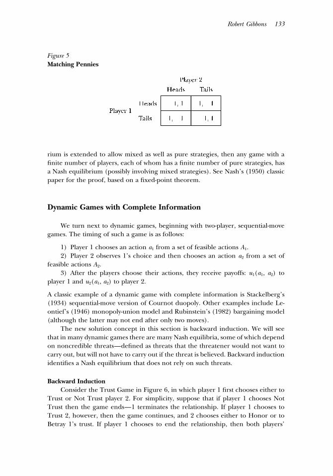
Other games, such as Matching Pennies in Figure 5, do not have a pair of strategiessatisfying the mutual-best-response definition of Nash equilibrium given above. Thedistinguishing feature of Matching Pennies is that each player would like to outguessthe other. Versions of this game also arise in poker, auditing and other settings. Inpoker, for example, the analogous question is how often to bluff: if player i is knownnever to bluff, then i’s opponents will fold whenever i bids aggressively, thereby makingit worthwhile for i to bluff on occasion; on the other hand, bluffing too often is also alosing strategy. Similarly, in auditing, if a subordinate worked diligently, then the bossprefers not to incur the cost of auditing the subordinate, but if the boss is not goingto audit, then the subordinate prefers to shirk, and so on.

In any game in which each player would like to outguess the other, there is nopair of strategies satisfying the definition of Nash equilibrium given above. Instead,the solution to such a game necessarily involves uncertainty about what the playerswill do. To model this uncertainty, we will refer to the actions in a player’s actionspace (Ai) as pure strategies, and we will define a mixed strategy to be a probabilitydistribution over some or all of the player’s pure strategies. A mixed strategy forplayer i is sometimes described as player i rolling dice to pick a pure strategy, butlater in the paper we will offer a much more plausible interpretation based on playerj’s uncertainty about the strategy player i will choose. Regardless of how one inter-prets mixed strategies, once the mutual-best-response definition of Nash equilib-


5 I owe the nonsexist, nonheterosexist player names to Matt Rabin. Allison Beezer noted, however, thatno amount of Rabin’s relabeling could overcome the game’s original name, so she suggested the DatingGame. Larry Samuelson suggested the updated choices available to the players.

There are of course many applications of this game, including political groups attempting to establisha constitution, firms attempting to establish an industry standard, and colleagues deciding which days towork at home.

Robert Gibbons 133

Figure 5Matching Pennies

rium is extended to allow mixed as well as pure strategies, then any game with afinite number of players, each of whom has a finite number of pure strategies, hasa Nash equilibrium (possibly involving mixed strategies). See Nash’s (1950) classicpaper for the proof, based on a fixed-point theorem.

Dynamic Games with Complete Information

We turn next to dynamic games, beginning with two-player, sequential-movegames. The timing of such a game is as follows:

1) Player 1 chooses an action a1 from a set of feasible actions A1.2) Player 2 observes 1’s choice and then chooses an action a2 from a set of

feasible actions A2.3) After the players choose their actions, they receive payoffs: u1(a1, a2) to

player 1 and u2(a1, a2) to player 2.

A classic example of a dynamic game with complete information is Stackelberg’s(1934) sequential-move version of Cournot duopoly. Other examples include Le-ontief’s (1946) monopoly-union model and Rubinstein’s (1982) bargaining model(although the latter may not end after only two moves).

The new solution concept in this section is backward induction. We will seethat in many dynamic games there are many Nash equilibria, some of which dependon noncredible threats—defined as threats that the threatener would not want tocarry out, but will not have to carry out if the threat is believed. Backward inductionidentifies a Nash equilibrium that does not rely on such threats.

Backward Induction


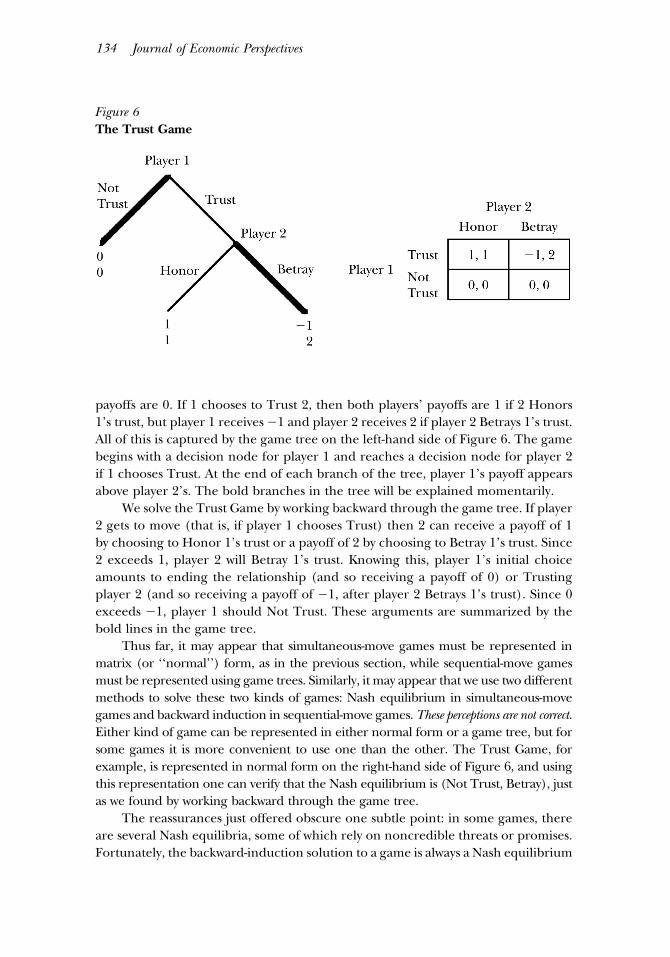
Consider the Trust Game in Figure 6, in which player 1 first chooses either toTrust or Not Trust player 2. For simplicity, suppose that if player 1 chooses NotTrust then the game ends—1 terminates the relationship. If player 1 chooses toTrust 2, however, then the game continues, and 2 chooses either to Honor or toBetray 1’s trust. If player 1 chooses to end the relationship, then both players’


Figure 6The Trust Game

payoffs are 0. If 1 chooses to Trust 2, then both players’ payoffs are 1 if 2 Honors1’s trust, but player 1 receives 01 and player 2 receives 2 if player 2 Betrays 1’s trust.All of this is captured by the game tree on the left-hand side of Figure 6. The gamebegins with a decision node for player 1 and reaches a decision node for player 2if 1 chooses Trust. At the end of each branch of the tree, player 1’s payoff appearsabove player 2’s. The bold branches in the tree will be explained momentarily.

We solve the Trust Game by working backward through the game tree. If player2 gets to move (that is, if player 1 chooses Trust) then 2 can receive a payoff of 1by choosing to Honor 1’s trust or a payoff of 2 by choosing to Betray 1’s trust. Since2 exceeds 1, player 2 will Betray 1’s trust. Knowing this, player 1’s initial choiceamounts to ending the relationship (and so receiving a payoff of 0) or Trustingplayer 2 (and so receiving a payoff of 01, after player 2 Betrays 1’s trust). Since 0exceeds 01, player 1 should Not Trust. These arguments are summarized by thebold lines in the game tree.

Thus far, it may appear that simultaneous-move games must be represented inmatrix (or ‘‘normal’’) form, as in the previous section, while sequential-move gamesmust be represented using game trees. Similarly, it may appear that we use two differentmethods to solve these two kinds of games: Nash equilibrium in simultaneous-movegames and backward induction in sequential-move games. These perceptions are not correct.Either kind of game can be represented in either normal form or a game tree, but forsome games it is more convenient to use one than the other. The Trust Game, forexample, is represented in normal form on the right-hand side of Figure 6, and using


this representation one can verify that the Nash equilibrium is (Not Trust, Betray), justas we found by working backward through the game tree.

The reassurances just offered obscure one subtle point: in some games, thereare several Nash equilibria, some of which rely on noncredible threats or promises.Fortunately, the backward-induction solution to a game is always a Nash equilibrium


Figure 7A Game that Relies on a Noncredible Threat

that does not rely on noncredible threats or promises. As an illustration of a Nashequilibrium that relies on a noncredible threat (but does not satisfy backward in-duction), consider the game tree and associated normal form in Figure 7. Workingbackward through this game tree shows that the backward-induction solution is forplayer 2 to play R� if given the move and for player 1 to play R. But the normalform reveals that there are two Nash equilibria: (R, R�) and (L, L�). The secondNash equilibrium exists because player 1’s best response to L� by 2 is to end thegame by choosing L. But (L, L�) relies on the noncredible threat by player 2 to playL� rather than R� if given the move. If player 1 believes 2’s threat, then 2 is off thehook because 1 will play L, but 2 would never want to carry out this threat if giventhe opportunity.

Backward induction can be applied in any finite-horizon game of completeinformation in which the players move one at a time and all previous moves arecommon knowledge before the next move is chosen. The method is simple: go tothe end of the game and work backward, one move at a time. In dynamic gameswith simultaneous moves or an infinite horizon, however, we cannot apply thismethod directly. We turn next to subgame-perfect Nash equilibrium, which extendsthe spirit of backward induction to such games.

Subgame-Perfect Nash EquilibriumSubgame-perfect Nash equilibrium is a refinement of Nash equilibrium; that is,

to be subgame-perfect, the players’ strategies must first be a Nash equilibrium andmust then fulfill an additional requirement. The point of this additional require-ment is, as with backward induction, to rule out Nash equilibria that rely on non-credible threats.

To provide an informal definition of subgame-perfect Nash equilibrium, we


return to the motivation for Nash equilibrium—namely, that a unique solution toa game-theoretic problem must satisfy Nash’s mutual-best-response requirement.In many dynamic games, the same argument can also be applied to certain piecesof the game, called subgames. A subgame is the piece of an original game thatremains to be played beginning at any point at which the complete history of the


play of the game thus far is common knowledge. In the one-shot Trust Game, forexample, the history of play is common knowledge after player 1 moves. The pieceof the game that then remains is very simple—just one move by player 2.

As a second example of a subgame (and, eventually, of subgame-perfect Nashequilibrium), consider Lazear and Rosen’s (1981) model of a tournament. First,the principal chooses two wages—WH for the winner, WL for the loser. Second, thetwo workers observe these wages and then simultaneously choose effort levels. Fi-nally, each worker’s output (which equals the worker’s effort plus noise) is observed,and the worker with the higher output earns WH. In this game, the history of playis common knowledge after the principal chooses the wages. The piece of the gamethat then remains is the effort-choice game between the workers.

Because the workers’ effort-choice game has simultaneous moves, we cannotgo to the end of the game and work backward one move at a time, as with backwardinduction. (If we go to the end of the game, which worker’s move should we analyzefirst?) Instead, we analyze both workers’ moves together. That is, we analyze theentire subgame that remains after the principal sets the wages by solving for theNash equilibrium in the workers’ effort-choice game given arbitrary wages chosenby the principal. Given the workers’ equilibrium response to these arbitrary wages,we can then work backward, solving the principal’s problem: choose wages thatmaximize expected profit given the workers’ equilibrium response. This processyields the subgame-perfect Nash equilibrium of the tournament game.

There typically are other Nash equilibria of the tournament game that arenot subgame-perfect. For example, the principal might pay very high wages be-cause the workers both threaten to shirk if she pays anything less. Solving forthe workers’ equilibrium response to an arbitrary pair of wages reveals that thisthreat is not credible. This solution process illustrates Selten’s (1965) definitionof a subgame-perfect Nash equilibrium: a Nash equilibrium (of the game aswhole) is subgame-perfect if the players’ strategies constitute a Nash equilibriumin every subgame.6

Repeated GamesWhen people interact over time, threats and promises concerning future

behavior may influence current behavior. Repeated games capture this fact oflife, and hence have been applied more broadly than any other game-theoreticmodel (by my armchair count)—not only in virtually every field of economicsbut also in finance, law, marketing, political science and sociology.

In this section, we analyze the infinitely repeated Trust Game, borrowed fromKreps’s (1990a) analysis of corporate culture. All previous outcomes are knownbefore the next period’s Trust Game is played. Both players share the interest rate

7


r per period. Consider the following ‘‘trigger’’ strategies:

6 Any finite game has a subgame-perfect Nash equilibrium, possibly involving mixed strategies, becauseeach subgame is itself a finite game and hence has a Nash equilibrium.7 The interest rate r can be interpreted as reflecting both the rate of time preference and the probabilitythat the current period will be the last, so that the ‘‘infinitely repeated’’ game ends at a random date.

Robert Gibbons 137

Player 1: In the first period, play Trust. Thereafter, if all moves in all pre-vious periods have been Trust and Honor, play Trust; otherwise, play NotTrust.

Player 2: If given the move this period, play Honor if all moves in all previousperiods have been Trust and Honor; otherwise, play Betray.

Recall that in the one-shot version of the Trust Game, backward inductionyields (Not Trust, Betray), with payoffs of (0, 0). Given the trigger strategiesstated above for the repeated game, this backward-induction outcome of thestage game will be the ‘‘punishment’’ outcome if cooperation collapses in therepeated game. Under these trigger strategies, the payoffs from ‘‘cooperation’’are (1, 1), but cooperation creates an incentive for ‘‘defection,’’ at least forplayer 2: if player 1 chooses Trust, player 2’s one-period payoff would be max-imized by choosing to Betray, producing payoffs of (01, 2). Thus, player 2 willcooperate if the present value of the payoffs from cooperation (1 ineach period) exceeds the present value of the payoffs from detection followedby punishment (2 immediately, but 0 thereafter). The former presentvalue exceeds the latter if the interest rate is sufficiently small (here,r ° 1).8

What about player 1? Suppose player 2 is playing his strategy given above.Because player 1 moves first, she has no chance to defect, in the sense of cheat-ing while player 2 attempts to cooperate. The only possible deviation for player1 is to play Not Trust, in which case player 2 does not get the move that period.But 2’s strategy then specifies that any future Trusts will be met with Betrayal.Thus, by playing Not Trust, player 1 gets 0 this period and 0 thereafter (be-cause playing Not Trust forever after is 1’s best response to 2’s anticipatedBetrayal of Trust). So if player 2 is playing his strategy given above, then it isoptimal for player 1 to play hers. Thus, if the interest rate is sufficiently small,then the trigger strategies stated above are a Nash equilibrium of the repeatedgame.9

The general point is that cooperation is prone to defection—otherwise weshould call it something else, such as a happy alignment of the players’ self-interests.But in some circumstances, defection can be met with punishment, in which casea potential defector must weigh the present value of continued cooperation againstthe short-term gain from defection followed by the long-term loss from punishment.If the players are sufficiently patient (that is, the interest rate is sufficiently small),then cooperation can occur in an equilibrium of the repeated game when it cannotin the one-shot game.


8 If player 1 is playing her strategy given above, then it is a best response for player 2 to play his strategyif {1 / (1/r)}1 ¢ 2 / (1/r)·0, or r ° 1. More generally, if a player’s payoffs (per period) are C fromcooperation, D from defection and P from punishment, then the player has an incentive to cooperateif {1 / (1/r)}C ¢ D / (1/r)P, or r ° (C 0 P)/(D 0 C).9 In fact, this Nash equilibrium of the repeated game is subgame-perfect.


Static Games with Incomplete Information

We turn next to games with incomplete information, also called Bayesian games.In a game of complete information, the players’ payoff functions are commonknowledge, whereas in a game of incomplete information at least one player isuncertain about another player’s payoff function. One common example of a staticgame of incomplete information is a sealed-bid auction: each bidder knows his orher own valuation for the good being sold, but does not know any other bidder’svaluation; bids are submitted in sealed envelopes, so the players’ moves are effec-tively simultaneous. Most economically interesting Bayesian games are dynamic,however, because the existence of private information leads naturally to attemptsby informed parties to communicate (or mislead) and to attempts by uninformedparties to learn and respond.

We first use the idea of incomplete information to provide a new interpretationfor mixed-strategy Nash equilibria in games with complete information—an inter-pretation of player i’s mixed strategy in terms of player j’s uncertainty about i’saction, rather than in terms of actual randomization on i’s part. Using this simplemodel as a template, we then define a static Bayesian game and a Bayesian Nashequilibrium. Reassuringly, we will see that a Bayesian Nash equilibrium is simply aNash equilibrium in a Bayesian game: the players’ strategies must be best responsesto each other.

Mixed Strategies ReinterpretedRecall that in the Dating Game discussed earlier, there are two pure-strategy

Nash equilibria: (Steak, Red Wine) and (Chicken, White Wine). There is also amixed-strategy Nash equilibrium, in which Chris chooses Steak with probability 2

3

and Chicken with probability , and Pat chooses White Wine with probability and1 23 3

Red Wine with probability . To verify that these mixed strategies constitute a Nash13

equilibrium, check that given Pat’s strategy, Chris is indifferent between the purestrategies of Steak and Chicken and so also indifferent among all probability dis-tributions over these pure strategies. Thus, the mixed strategy specified for Chrisis one of a continuum of best responses to Pat’s strategy. The same is true for Pat,so the two mixed strategies are a Nash equilibrium.

Now suppose that, although they have known each other for quite some time,Chris and Pat are not quite sure of each other’s payoffs, as shown in Figure 8. Chris’spayoff from Steak with Red Wine is now 2 / tc, where tc is privately known by Chris;Pat’s payoff from Chicken with White Wine is now 2 / tp, where tp is privately knownby Pat; and tc and tp are independent draws from a uniform distribution on [0, x].The choice of a uniform distribution is only for convenience, but we do have in


mind that the values of tc and tp only slightly perturb the payoffs in the originalgame, so think of x as small. All the other payoffs are the same as in the originalcomplete-information game.

We will construct a pure-strategy Bayesian Nash equilibrium of this incomplete-information version of the Dating Game in which Chris chooses Steak if tc exceeds


Figure 8The Dating Game with Incomplete Information

a critical value, c, and chooses Chicken otherwise, and Pat chooses White Wine iftp exceeds a critical value, p, and chooses Red Wine otherwise. In such an equilib-rium, Chris chooses Steak with probability (x 0 c)/x, and Pat chooses White Winewith probability (x 0 p)/x. (For example, if the critical value c is nearly x, then theprobability that tc will exceed c is almost zero.) We will show that as the incompleteinformation disappears—that is, as x approaches zero—the players’ behavior inthis pure-strategy Bayesian Nash equilibrium of the incomplete-information gameapproaches their behavior in the mixed-strategy Nash equilibrium in the originalcomplete-information game. That is, both (x 0 c)/x and (x 0 p)/x approach as x2

3

approaches zero.Suppose that Pat will play the strategy described above for the incomplete-

information game. Chris can then compute that Pat chooses White Wine with prob-ability (x 0 p)/x and Red with probability p/x, so Chris’s expected payoffs fromchoosing Steak and from choosing Chicken are p(2 / tc)/x and (x 0 p)/x, respec-tively. Thus, Chris’s best response to Pat’s strategy has the form described above:choosing Steak has the higher expected payoff if and only if tc ¢ (x 0 3p)/p å c.Similarly, given Chris’s strategy, Pat can compute that Chris chooses Steak withprobability (x 0 c)/x and Chicken with probability c/x, so Pat’s expected payoffsfrom choosing White Wine and from choosing Red Wine are c(2 / tp)/x and(x 0 c)/x, respectively. Thus, choosing White Wine has the higher expected payoffif and only if tp ¢ (x 0 3c)/c å p.

We have now shown that Chris’s strategy (namely, Steak if and only iftc ¢ c) and Pat’s strategy (namely, White Wine if and only if tp ¢ p) are bestresponses to each other if and only if (x 0 3p)/p Å c and (x 0 3c)/c Å p. Solvingthese two equations for p and c shows that the probability that Chris choosesSteak, namely, (x 0 c)/x, and the probability that Pat chooses White Wine,namely, (x 0 p)/x, are equal. This probability approaches as x approaches zero2

3


(by application of l’Hopital’s rule). Thus, as the incomplete information dis-appears, the players’ behavior in this pure-strategy Bayesian Nash equilibriumof the incomplete-information game approaches their behavior in the mixed-strategy Nash equilibrium in the original game of complete information.

Harsanyi (1973) showed that this result is quite general: a mixed-strategy Nash


equilibrium in a game of complete information can (almost always) be interpretedas a pure-strategy Bayesian Nash equilibrium in a closely related game with a littlebit of incomplete information. Put more evocatively, the crucial feature of a mixed-strategy Nash equilibrium is not that player j chooses a strategy randomly, but ratherthat player i is uncertain about player j’s choice; this uncertainty can arise eitherbecause of randomization or (more plausibly) because of a little incompleteinformation.

Static Bayesian Games and Bayesian Nash EquilibriumRecall from the first section that in a two-player, simultaneous-move game of

complete information, first the players simultaneously choose actions (player ichooses ai from the feasible set Ai) and then payoffs ui(ai, aj) are received. Todescribe a two-player, simultaneous-move game of incomplete information, the firststep is to represent the idea that each player knows his or her own payoff functionbut may be uncertain about the other player’s payoff function. Let player i’s possiblepayoff functions be represented by ui(ai, aj; ti), where ti is called player i’s type andbelongs to a set of possible types (or type space) Ti. Each type ti corresponds to adifferent payoff function that player i might have. In an auction, for example, aplayer’s payoff depends not only on all the players’ bids (that is, the players’ actionsai and aj) but also on the player’s own valuation for the good being auctioned (thatis, the player’s type ti).

Given this definition of a player’s type, saying that player i knows his or herown payoff function is equivalent to saying that player i knows his or her type.Likewise, saying that player i may be uncertain about player j’s payoff function isequivalent to saying that player i may be uncertain about player j’s type tj. (In anauction, player i may be uncertain about player j’s valuation for the good.) We usethe probability distribution p(tjÉti) to denote player i’s belief about player j’s type,tj, given player i’s knowledge of her own type, ti. For notational simplicity we assume(as in most of the literature) that the players’ types are independent, in which casep(tj É ti) does not depend on ti, so we can write player i’s belief as p(tj).10

Joining these new concepts of types and beliefs with the familiar elements ofa static game of complete information yields a static Bayesian game, as first definedby Harsanyi (1967, 1968a,b). The timing of a two-player static Bayesian game is asfollows:

1) Nature draws a type vector t Å (t1, t2), where ti is independently drawn fromthe probability distribution p(ti) over player i’s set of possible types Ti.

2) Nature reveals ti to player i but not to player j.


10 As an example of correlated types, imagine that two firms are racing to develop a new technology.Each firm’s chance of success depends in part on how difficult the technology is to develop, which isnot known. Each firm knows only whether it has succeeded, not whether the other has. If firm 1 hassucceeded, however, then it is more likely that the technology is easy to develop and so also more likelythat firm 2 has succeeded. Thus, firm 1’s belief about firm 2’s type depends on firm 1’s knowledge ofits own type.

Robert Gibbons 141

3) The players simultaneously choose actions, player i choosing ai from thefeasible set Ai.

4) Payoffs ui(ai, aj; ti) are received by each player.11

It may be helpful to check that the Dating Game with incomplete informationdescribed above is a simple example of this abstract definition of a static Bayesiangame.

We now need to define an equilibrium concept for static Bayesian games. Todo so, we must first define the players’ strategy spaces in such a game, after whichwe will define a Bayesian Nash equilibrium to be a pair of strategies such that eachplayer’s strategy is a best response to the other player’s strategy. That is, given theappropriate definition of a strategy in a static Bayesian game, the appropriate def-inition of equilibrium (now called Bayesian Nash equilibrium) is just the familiardefinition from Nash.12

A strategy in a static Bayesian game is an action rule, not just an action. Moreformally, a (pure) strategy for player i specifies a feasible action (ai) for each ofplayer i’s possible types (ti). In the Dating Game with incomplete information, forexample, Chris’s strategy was a rule specifying Chris’s action for each possible valueof tc: Steak if tc exceeds a critical value, c, and Chicken otherwise. Similarly, in anauction, a bidder’s strategy is a rule specifying the player’s bid for each possiblevaluation the bidder might have for the good.

In a static Bayesian game, player 1’s strategy is a best response to player 2’s if,for each of player 1’s types, the action specified by 1’s action rule for that typemaximizes 1’s expected payoff, given 1’s belief about 2’s type and given 2’s actionrule. In the Bayesian Nash equilibrium we constructed in the Dating Game, forexample, there was no incentive for Chris to change even one action by one type,given Chris’s belief about Pat’s type and given Pat’s action rule (namely, chooseWhite Wine if tp exceeds a critical value, p, and choose Red Wine otherwise). Like-wise, in a Bayesian Nash equilibrium of a two-bidder auction, bidder 1 has noincentive to change even one bid by one valuation-type, given bidder 1’s belief aboutbidder 2’s type and given bidder 2’s bidding rule.13

11 There are games in which one player has private information not only about his or her own payofffunction but also about another player’s payoff function. As an example, consider an asymmetric-information Cournot model in which costs are common knowledge, but one firm knows the level ofdemand and the other does not. Since the level of demand affects both players’ payoff functions, theinformed firm’s type enters the uninformed firm’s payoff function. To allow for such information struc-tures, the payoff functions in a Bayesian game can be written as ui(ai, aj; ti, tj).12 Given the close connection between Nash equilibrium and Bayesian Nash equilibrium, it should notbe surprising that a Bayesian Nash equilibrium exists in any finite Bayesian game.13 It may seem strange to define equilibrium in terms of action rules. In an auction, for example, why


can’t a bidder simply consider what bid to make given her actual valuation? Why does it matter whatbids she would have made given other valuations? To see through this puzzle, note that for bidder 1 tocompute an optimal bid, bidder 1 needs a conjecture about bidder 2’s entire bidding rule. And todetermine whether even one bid from this rule is optimal, bidder 2 would need a conjecture aboutbidder 1’s entire bidding rule. Akin to a rational expectations equilibrium, these conjectured biddingrules must be correct in a Bayesian Nash equilibrium.


Dynamic Games with Incomplete Information

As noted earlier, the existence of private information leads naturally to at-tempts by informed parties to communicate (or to mislead) and to attempts byuninformed parties to learn and respond. The simplest model of such attempts isa signaling game: there are two players—one with private information, the otherwithout; and there are two stages in the game—a signal sent by the informed party,followed by a response taken by the uninformed party. In Spence’s (1973) classicmodel, for example, the informed party is a worker with private information abouthis or her productive ability, the uninformed party is a potential employer (or amarket of same), the signal is education, and the response is a wage offer.

Richer dynamic Bayesian games allow for reputations to be developed, main-tained or milked. In the first such analysis, Kreps, Milgrom, Roberts and Wilson(1982) showed that a finitely repeated prisoners’ dilemma that begins with a littlebit of (the right kind of) private information can have equilibrium cooperation inall but the last few periods. In contrast, a backward-induction argument shows thatequilibrium cooperation cannot occur in any round of a finitely repeated prisoners’dilemma under complete information, because knowing that cooperation will breakdown in the last round causes it to break down in the next-to-last round, and so onback to the first round. Signaling games, reputation games and other dynamicBayesian games (like bargaining games) have been very widely applied in manyfields of economics and in accounting, finance, law, marketing and political science.For example, see Benabou and Laroque (1992) on insiders and gurus in financialmarkets, Cramton and Tracy (1992) on strikes and Rogoff (1989) on monetarypolicy.

Perfect Bayesian EquilibriumTo analyze dynamic Bayesian games, we introduce a fourth equilibrium con-

cept: perfect Bayesian equilibrium. The crucial new feature of perfect Bayesianequilibrium is due to Kreps and Wilson (1982): beliefs are elevated to the level ofimportance of strategies in the definition of equilibrium. That is, the definition ofequilibrium no longer consists of just a strategy for each player but now also in-cludes a belief for each player whenever the player has the move but is uncertainabout the history of prior play.14 The advantage of making the players’ beliefs anexplicit part of the equilibrium is that, just as we previously insisted that the playerschoose credible (that is, subgame-perfect) strategies, we can now also insist thatthey hold reasonable beliefs.

14


Kreps and Wilson (1982) formalize this perspective on equilibrium by defining sequential equilibrium,an equilibrium concept that is equivalent to perfect Bayesian equilibrium in many economic applicationsbut in some cases is slightly stronger. Sequential equilibrium is more complicated to define and to applythan perfect Bayesian equilibrium, so most authors now use the latter. Kreps and Wilson show that anyfinite game (with or without private information) has a sequential equilibrium, so the same can be saidfor perfect Bayesian equilibrium.


Figure 9Why Players’ Beliefs are as Important as their Strategies

To illustrate why the players’ beliefs are as important as their strategies,consider the example in Figure 9. (This example shows that perfect Bayesianequilibrium refines subgame-perfect Nash equilibrium; we return to dynamicBayesian games in the next subsection.) First, player 1 chooses among threeactions: L, M and R. If player 1 chooses R then the game ends without a moveby player 2. If player 1 chooses either L or M then player 2 learns that R was notchosen (but not which of L or M was chosen) and then chooses between twoactions, L� and R�, after which the game ends. (The dashed line connectingplayer 2’s two decision nodes in the game tree on the left of Figure 9 indicatesthat if player 2 gets the move, player 2 does not know which node has beenreached—that is, whether player 1 has chosen L or M. The probabilities p and1 0 p attached to player 2’s decision nodes will be explained below.) Payoffs aregiven in the game tree.

The normal-form representation of this game on the right-hand side of Figure9 reveals that there are two pure-strategy Nash equilibria: (L, L�) and (R, R�). Wefirst ask whether these Nash equilibria are subgame-perfect. Because a subgame isdefined to begin when the history of prior play is common knowledge, there areno subgames in the game tree above. (After player 1’s decision node at the begin-ning of the game, there is no point at which the complete history of play is commonknowledge: the only other nodes are player 2’s, and if these nodes are reached,then player 2 does not know whether the previous play was L or M.) If a game hasno subgames, then the requirement of subgame-perfection—namely, that the play-ers’ strategies constitute a Nash equilibrium on every subgame—is trivially satisfied.Thus, in any game that has no subgames the definition of subgame-perfect Nash


equilibrium is equivalent to the definition of Nash equilibrium, so in this exampleboth (L, L�) and (R, R�) are subgame-perfect Nash equilibria. Nonetheless, (R, R�)clearly depends on a noncredible threat: if player 2 gets the move, then playing L�

dominates playing R�, so player 1 should not be induced to play R by 2’s threat toplay R� if given the move.


One way to strengthen the equilibrium concept so as to rule out the sub-game-perfect Nash equilibrium (R, R�) is to impose two requirements.

Requirement 1: Whenever a player has the move and is uncertain about thehistory of prior play, the player must have a belief over the set of feasible historiesof play.

Requirement 2: Given their beliefs, the players’ strategies must be sequentiallyrational. That is, whenever a player has the move, the player’s action (and theplayer’s strategy from then on) must be optimal given the player’s belief at thatpoint (and the other players’ strategies from then on).

In the example above, Requirement 1 implies that if player 2 gets the move, thenplayer 2 must have a belief about whether player 1 has played L or M. This beliefis represented by the probabilities p and 1 0 p attached to the relevant nodes inthe game tree. Given player 2’s belief, the expected payoff from playing R� isp·0 / (1 0 p)·1 Å 1 0 p, while the expected payoff from playing L� isp·1 / (1 0 p)·2 Å 2 0 p. Since 2 0 p ú 1 0 p for any value of p, Requirement2 prevents player 2 from choosing R�. Thus, simply requiring that each playerhave a belief and act optimally given this belief suffices to eliminate the implau-sible equilibrium (R, R�) in this example.

What about the other subgame-perfect Nash equilibrium, (L, L�)? Require-ment 1 dictates that player 2 have a belief but does not specify what it should be.In the spirit of rational expectations, however, player 2’s belief in this equilibriumshould be p Å 1. We state this idea a bit more formally as

Requirement 3: Where possible, beliefs should be determined by Bayes’ rule fromthe players’ equilibrium strategies.

We give other examples of Requirement 3 below.In simple economic applications, including the signaling games discussed be-

low, Requirements 1 through 3 constitute the definition of perfect Bayesian equilib-rium. In richer applications, more requirements need to be imposed to eliminateimplausible equilibria.15

Signaling GamesWe now return to dynamic Bayesian games, where we will apply perfect Bayes-

ian equilibrium. For simplicity, we restrict attention to (finite) signaling games,which have the following timing:

1) Nature draws a type ti for the Sender from a set of feasible types T Å {t1,. . . , tI} according to a probability distribution p(ti).


15 To give a sense of the issues not addressed by Requirements 1 through 3, suppose players 2 and 3 haveobserved the same events, and then both observe a deviation from the equilibrium by player 1. Shouldplayers 2 and 3 hold the same belief about earlier unobserved moves by player 1? Fudenberg and Tirole(1991a) give a formal definition of perfect Bayesian equilibrium for a broad class of dynamic Bayesiangames and provide conditions under which their perfect Bayesian equilibrium is equivalent to Kreps andWilson’s (1982) sequential equilibrium.

Robert Gibbons 145

Figure 10The Beer and Quiche Signaling Game

2) The Sender observes ti and then chooses a message mj from a set of feasiblemessages M Å {m1, . . . , mJ}.

3) The Receiver observes mj (but not ti) and then chooses an action ak from aset of feasible actions A Å {a1, . . . , aK}.

4) Payoffs are given by US(ti, mj, ak) and UR(ti, mj, ak).

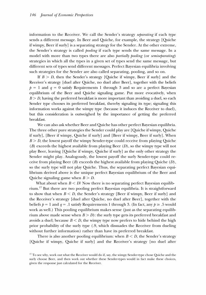
In Cho and Kreps’s (1987) ‘‘Beer and Quiche’’ signaling game, shown in Figure10, the type, message and action spaces (T, M and A, respectively) all have only twoelements. While most game trees start at the top, a signaling game starts in the middle,with a move by Nature that determines the Sender’s type: here t1 Å ‘‘wimpy’’ (withprobability .1) or t2 Å ‘‘surly’’ (with probability .9).16 Both Sender types then have thesame choice of messages—Quiche or Beer (as alternative breakfasts). The Receiverobserves the message but not the type. (As above, the dashed line connecting two ofthe Receiver’s two decision nodes indicates that the Receiver knows that one of thenodes in this ‘‘information set’’ was reached, but does not know which node—that is,the Receiver observes the Sender’s breakfast but not his type.) Finally, following eachmessage, the Receiver chooses between two actions—to duel or not to duel with theSender.

The qualitative features of the payoffs are that the wimpy type would prefer tohave quiche for breakfast, the surly type would prefer to have beer, both types wouldprefer not to duel with the Receiver, and the Receiver would prefer to duel withthe wimpy type but not to duel with the surly type. Specifically, the preferred break-fast is worth B ú 0 for both sender types, avoiding a duel is worth D ú 0 for bothSender types, and the payoff from a duel with the wimpy (respectively, surly) typeis 1 (respectively, 01) for the Receiver; all other payoffs were zero.


The point of a signaling game is that the Sender’s message may convey

16 Readers over the age of 35 may recognize that the labels in this game were inspired by Real Men Don’tEat Quiche, a highly visible book when this example was conceived.


information to the Receiver. We call the Sender’s strategy separating if each typesends a different message. In Beer and Quiche, for example, the strategy [Quicheif wimpy, Beer if surly] is a separating strategy for the Sender. At the other extreme,the Sender’s strategy is called pooling if each type sends the same message. In amodel with more than two types there are also partially pooling (or semiseparating)strategies in which all the types in a given set of types send the same message, butdifferent sets of types send different messages. Perfect Bayesian equilibria involvingsuch strategies for the Sender are also called separating, pooling, and so on.

If B ú D, then the Sender’s strategy [Quiche if wimpy, Beer if surly] and theReceiver’s strategy [duel after Quiche, no duel after Beer], together with the beliefsp Å 1 and q Å 0 satisfy Requirements 1 through 3 and so are a perfect Bayesianequilibrium of the Beer and Quiche signaling game. Put more evocatively, whenB ú D, having the preferred breakfast is more important than avoiding a duel, so eachSender type chooses its preferred breakfast, thereby signaling its type; signaling thisinformation works against the wimpy type (because it induces the Receiver to duel),but this consideration is outweighed by the importance of getting the preferredbreakfast.

We can also ask whether Beer and Quiche has other perfect Bayesian equilibria.The three other pure strategies the Sender could play are [Quiche if wimpy, Quicheif surly], [Beer if wimpy, Quiche if surly] and [Beer if wimpy, Beer if surly]. WhenB ú D, the lowest payoff the wimpy Sender-type could receive from playing Quiche(B) exceeds the highest available from playing Beer (D), so the wimpy type will notplay Beer, leaving [Quiche if wimpy, Quiche if surly] as the only other strategy theSender might play. Analogously, the lowest payoff the surly Sender-type could re-ceive from playing Beer (B) exceeds the highest available from playing Quiche (D),so the surly type will not play Quiche. Thus, the separating perfect Bayesian equi-librium derived above is the unique perfect Bayesian equilibrium of the Beer andQuiche signaling game when B ú D.

What about when B õ D? Now there is no separating perfect Bayesian equilib-rium.17 But there are two pooling perfect Bayesian equilibria. It is straightforwardto show that when B õ D, the Sender’s strategy [Beer if wimpy, Beer if surly] andthe Receiver’s strategy [duel after Quiche, no duel after Beer], together with thebeliefs p Å 1 and q Å .1 satisfy Requirements 1 through 3. (In fact, any p ¢ .5 wouldwork as well.) This pooling equilibrium makes sense (just as the separating equilib-rium above made sense when B ú D): the surly type gets its preferred breakfast andavoids a duel; because B õ D, the wimpy type now prefers to hide behind the highprior probability of the surly type (.9, which dissuades the Receiver from duelingwithout further information) rather than have its preferred breakfast.

There is also another pooling equilibrium: when B õ D, the Sender’s strategy


[Quiche if wimpy, Quiche if surly] and the Receiver’s strategy [no duel after

17 To see why, work out what the Receiver would do if, say, the wimpy Sender-type chose Quiche and thesurly choose Beer, and then work out whether these Sender-types would in fact make these choices,given the response just calculated for the Receiver.


Quiche, duel after Beer], together with the beliefs p Å .1 and q Å 1 satisfy Require-ments 1 through 3. (In fact, any q ¢ .5 would work as well.) Cho and Kreps arguethat the Receiver’s belief in this equilibrium is counterintuitive. Their ‘‘IntuitiveCriterion’’ refines perfect Bayesian equilibrium by putting additional restrictionson beliefs (beyond Requirement 3) that rule out this pooling equilibrium (but notthe previous pooling equilibrium, in which both types choose Beer).

Further Reading

I hope this paper has clearly defined the four major classes of games and theirsolution concepts, as well as sketched the motivation for and connections amongthese concepts. This may be enough to allow some applied economists to grapplewith game-theoretic work in their own research areas, but I hope to have interestedat least a few readers in more than this introduction.

An economist seeking further reading on game theory has the luxury of a greatdeal of choice—at least eight new books, as well as at least two earlier texts, one now inits second edition. (I apologize for excluding several other books written either for orby noneconomists, as well as any books by and for economists that have escaped myattention.) These ten books are Binmore (1992), Dixit and Nalebuff (1991), Friedman(1990), Fudenberg and Tirole (1991b), Gibbons (1992), Kreps (1990b), McMillan(1992), Myerson (1991), Osborne and Rubinstein (1994) and Rasmussen (1989). Thesebooks are all excellent, but I think it fair to say that different readers will find differentbooks appropriate, depending on the reader’s background and goals. At the risk ofoffending my fellow authors, let me hazard some characterizations and suggestions.

Roughly speaking, some books emphasize theory, others economic applica-tions, and still others ‘‘the real world.’’ Given a book’s emphasis, there is then aquestion regarding its level. I see Binmore, Friedman, Fudenberg-Tirole, Kreps,Myerson and Osborne-Rubinstein as books that emphasize theory. If I were tryingto transform a bright undergraduate into a game theorist (as distinct from an ap-plied modeler), I would start with either or both of Binmore and Kreps, and thenproceed to any or all of Friedman, Fudenberg-Tirole, Myerson and Osborne-Rubinstein. In contrast, I see Gibbons and Rasmussen (and, to some extent, Mc-Millan) as books that emphasize economic applications. Each is accessible to abright undergraduate, but could also provide the initial doctoral training for anapplied modeler and perhaps the full doctoral training for an applied economistwishing to consume (rather than construct) applied models. The next step for thosewho wish to construct such models might be to sample from Fudenberg-Tirole, as the


most applications oriented of the advanced theory books. Finally, I see Dixit-Nalebuff and McMillan as books that emphasize the real world (McMillan being moreclosely tied to applications from the economics literature). These are the texts to useto teach an undergraduate (or an MBA) to think strategically, although for this purposeone should also read the collected works of Thomas Schelling. These books would also


be useful additions to the training of an applied modeler, in the hope that the studentwould learn to keep his or her eye on the empirical ball.

All of this further reading is for economists seeking a deeper treatment of thetheory. I wish I could offer analogous recommendations for those seeking furtherreading on the many ways game theory has been used to build new theoreticalmodels, both inside and outside economics; this will have to await a future survey.More importantly, I eagerly await the first thorough assessment of how game-theoretic models in economics have fared when confronted with field data of the kindcommonly used to assess price-theoretic models. For an important step in a related
direction, see Roth and Kagel’s (1995) excellent Handbook of Experimental Economics,which describes laboratory evidence pertaining to many game-theoretic models.
t and Brad De Long, Alan Krueger and Timothy
� I thank Carl Shapiro for shaping this projecTaylor for helpful comments.
References

Benabou, Roland, and Guy Laroque, ‘‘UsingPrivileged Information to Manipulate Markets:Insiders, Gurus, and Credibility,’’ Quarterly Jour-nal of Economics, August 1992, 107, 921–58.

Binmore, Ken, Fun and Games: A Text on GameTheory. Lexington, Mass.: D. C. Heath & Co,1992.

Cho, In-Koo, and David Kreps, ‘‘SignalingGames and Stable Equilibria,’’ Quarterly Journal ofEconomics, May 1987, 102, 179–222.

Cournot, A., Recherches sur les Principes Mathe-matiques de la Theorie des Richesses. 1838. Englishedition, Bacon, N., ed., Researches into the Mathe-matical Principles of the Theory of Wealth. New York:Macmillan, 1897.

Cramton, Peter, and Joseph Tracy, ‘‘Strikesand Holdouts in Wage Bargaining: Theory andData,’’ American Economic Review, March 1992, 82,100–21.

Dixit, Avinash, and Barry Nalebuff, ThinkingStrategically: The Competitive Edge in Business, Poli-tics, and Everyday Life. New York: Norton, 1991.

Farber, Henry, ‘‘An Analysis of Final-Offer Ar-bitration,’’ Journal of Conflict Resolution, Decem-ber 1980, 35, 683–705.

/ av1 3006 0002 Mp 148 Friday Oct 27 13007

Friedman, James, Game Theory with Applicationsto Economics. 2nd ed., Oxford: Oxford UniversityPress, 1990.

Fudenberg, Drew, and Jean Tirole, ‘‘PerfectBayesian Equilibrium and Sequential Equilib-rium,’’ Journal of Economic Theory, April 1991a, 53,236–60.

Fudenberg, Drew, and Jean Tirole, Game The-ory. Cambridge, Mass.: Massachusetts Institute ofTechnology Press, 1991b.

Gibbons, Robert, Game Theory for Applied Econ-omists. Princeton, N.J.: Princeton UniversityPress, 1992.

Grossman, Sanford, and Oliver Hart, ‘‘Take-over Bids, the Free-Rider Problem, and the The-ory of the Corporation,’’ Bell Journal of Economics,Spring 1980, 11, 42–64.

Harsanyi, John, ‘‘Games with Incomplete In-formation Played by ‘Bayesian Players’: I. The Ba-sic Model,’’ Management Science, November 1967,14, 159–82.

Harsanyi, John, ‘‘Games with Incomplete In-formation Played by ‘Bayesian Players’: II. Bayes-ian Equilibrium Points,’’ Management Science, Jan-uary 1968a, 14, 320–34.

Harsanyi, John, ‘‘Games with Incomplete In-formation Played by ‘Bayesian Players’: III. TheBasic Probability Distribution of the Game,’’Management Science, March 1968b, 14, 486–502.

Harsanyi, John, ‘‘Games with Randomly Dis-turbed Payoffs: A New Rationale for Mixed Strat-egy Equilibrium Points,’’ International Journal ofGame Theory, 1973, 2:1, 1–23.

2:24 PM LP–JEP 0002

Hotelling, Harold, ‘‘Stability in Competition,’’Economic Journal, March 1929, 39, 41–57.

Kreps, David, ‘‘Corporate Culture and EconomicTheory.’’ In Alt, J., and K. Shepsle, eds., Perspectiveson Positive Political Economy. Cambridge: CambridgeUniversity Press, 1990a, pp. 90–143.

Kreps, David, Game Theory and Economic Mod-eling. Oxford: Oxford University Press, 1990b.

Kreps, David, and Robert Wilson, ‘‘SequentialEquilibrium,’’ Econometrica, July 1982, 50, 863–94.

Kreps, David, Paul Milgrom, John Roberts,and Robert Wilson, ‘‘Rational Cooperation inthe Finitely Repeated Prisoners’ Dilemma,’’ Jour-nal of Economic Theory, August 1982, 27, 245–52.

Lazear, Edward, and Sherwin Rosen, ‘‘Rank-Order Tournaments as Optimum Labor Con-tracts,’’ Journal of Political Economy, October 1981,89, 841–64.

Leontief, Wessily, ‘‘The Pure Theory of theGuaranteed Annual Wage Contract,’’ Journal ofPolitical Economy, February 1946, 54, 76–9.

McMillan, John, Games, Strategies, and Manag-ers. Oxford: Oxford University Press, 1992.

Myerson, Roger, Game Theory: Analysis of Conflict.Cambridge, Mass.: Harvard University Press, 1991.

/ av1 3006 0002 Mp 149 Friday Oct 27 123007

Nash, John, ‘‘Equilibrium Points in n-PersonGames,’’ Proceedings of the National Academy of Sci-ences, 1950, 36, 48–9.

Osborne, Martin, and Ariel Rubinstein, ACourse in Game Theory. Cambridge, Mass.: Massa-chusetts Institute of Technology Press, 1994.

Robert Gibbons 149

Rasmussen, Eric, Games and Information: An In-troduction to Game Theory. New York: Basil Black-well, 1989.

Rogoff, Kenneth, ‘‘Reputation, Coordination,and Monetary Policy.’’ In Barro, R., ed., ModernBusiness Cycle Theory. Cambridge, Mass.: HarvardUniversity Press, 1989, pp. 236–64.

Roth, Alvin, and John Kagel, Handbook of Ex-perimental Economics. Princeton, N.J.: PrincetonUniversity Press, 1995.

Rubinstein, Ariel, ‘‘Perfect Equilibrium in aBargaining Model,’’ Econometrica, January 1982,50, 97–109.

Selten, R., ‘‘Spieltheoretische Behandlung ei-nes Oligopolmodells mit Nachfragetragheit,’’Zeitschrift fur Gesamte Staatswissenschaft, 1965, 121,301–24.

Spence, A. Michael, ‘‘Job Market Signaling,’’Quarterly Journal of Economics, August 1973, 87,

:24 PM LP–JEP 0002

355–74.von Stackelberg, H., Marktform und Gleichgew-

icht. Vienna: Julius Springer, 1934.Young, H. Peyton, ‘‘The Economics of Con-

vention,’’ Journal of Economic Perspectives, Spring1996, 10, 105–22.

an introduction to applicable game theory - home |...

Documents