an introduction to bayesian nonparametric modelling
TRANSCRIPT
An Introduction toBayesian Nonparametric Modelling
Yee Whye Teh
Gatsby Computational Neuroscience UnitUniversity College London
October, 2009 / Toronto
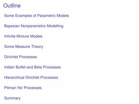
Outline
Some Examples of Parametric Models
Bayesian Nonparametric Modelling
Infinite Mixture Models
Some Measure Theory
Dirichlet Processes
Indian Buffet and Beta Processes
Hierarchical Dirichlet Processes
Pitman-Yor Processes
Summary
Outline
Some Examples of Parametric Models
Bayesian Nonparametric Modelling
Infinite Mixture Models
Some Measure Theory
Dirichlet Processes
Indian Buffet and Beta Processes
Hierarchical Dirichlet Processes
Pitman-Yor Processes
Summary
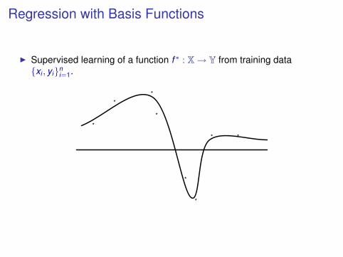
Regression with Basis Functions
I Supervised learning of a function f ∗ : X→ Y from training data{xi , yi}n
i=1.
**
*
*
*
*
*
*
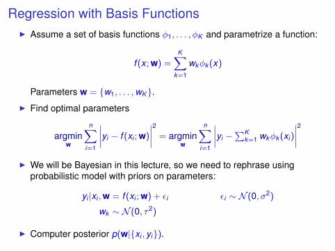
Regression with Basis FunctionsI Assume a set of basis functions φ1, . . . , φK and parametrize a function:
f (x ; w) =K∑
k=1
wkφk (x)
Parameters w = {w1, . . . ,wK}.I Find optimal parameters
argminw
n∑i=1
∣∣∣∣yi − f (xi ; w)
∣∣∣∣2 = argminw
n∑i=1
∣∣∣∣yi −∑K
k=1 wkφk (xi )
∣∣∣∣2I We will be Bayesian in this lecture, so we need to rephrase using
probabilistic model with priors on parameters:
yi |xi ,w = f (xi ; w) + εi εi ∼ N (0, σ2)
wk ∼ N (0, τ2)
I Computer posterior p(w|{xi , yi}).
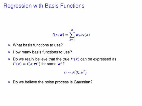
Regression with Basis Functions
f (x ; w) =K∑
k=1
wkφk (x)
I What basis functions to use?
I How many basis functions to use?
I Do we really believe that the true f ∗(x) can be expressed asf ∗(x) = f (x ; w∗) for some w∗?
εi ∼ N (0, σ2)
I Do we believe the noise process is Gaussian?
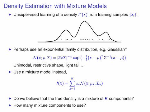
Density Estimation with Mixture ModelsI Unsupervised learning of a density f ∗(x) from training samples {xi}.
* ** * ** * ** *** ****
I Perhaps use an exponential family distribution, e.g. Gaussian?
N (x ;µ,Σ) = |2πΣ|− 12 exp
(− 12 (x − µ)>Σ−1(x − µ)
)Unimodal, restrictive shape, light tail...
I Use a mixture model instead,
f (x) =K∑
k=1
πkN (x ;µk ,Σk )
I Do we believe that the true density is a mixture of K components?I How many mixture components to use?
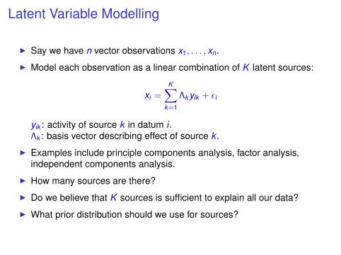
Latent Variable Modelling
I Say we have n vector observations x1, . . . , xn.
I Model each observation as a linear combination of K latent sources:
xi =K∑
k=1
Λk yik + εi
yik : activity of source k in datum i .Λk : basis vector describing effect of source k .
I Examples include principle components analysis, factor analysis,independent components analysis.
I How many sources are there?
I Do we believe that K sources is sufficient to explain all our data?
I What prior distribution should we use for sources?
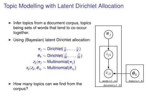
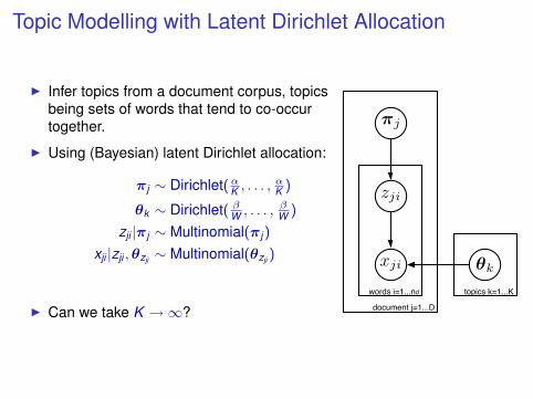
Topic Modelling with Latent Dirichlet Allocation
I Infer topics from a document corpus, topicsbeing sets of words that tend to co-occurtogether.
I Using (Bayesian) latent Dirichlet allocation:
πj ∼ Dirichlet(αK , . . . ,αK )
θk ∼ Dirichlet( βW , . . . , βW )
zji |πj ∼ Multinomial(πj )
xji |zji ,θzji ∼ Multinomial(θzji )
I How many topics can we find from thecorpus?
topics k=1...K
document j=1...D
words i=1...nd
πj
zji
xji θk
Outline
Some Examples of Parametric Models
Bayesian Nonparametric Modelling
Infinite Mixture Models
Some Measure Theory
Dirichlet Processes
Indian Buffet and Beta Processes
Hierarchical Dirichlet Processes
Pitman-Yor Processes
Summary
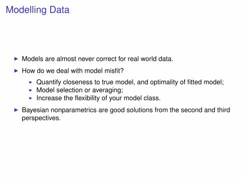
Modelling Data
I Models are almost never correct for real world data.
I How do we deal with model misfit?
I Quantify closeness to true model, and optimality of fitted model;I Model selection or averaging;I Increase the flexibility of your model class.
I Bayesian nonparametrics are good solutions from the second and thirdperspectives.
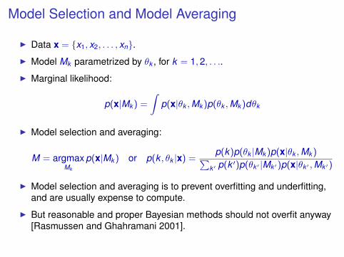
Model Selection and Model Averaging
I Data x = {x1, x2, . . . , xn}.I Model Mk parametrized by θk , for k = 1,2, . . ..
I Marginal likelihood:
p(x|Mk ) =
∫p(x|θk ,Mk )p(θk ,Mk )dθk
I Model selection and averaging:
M = argmaxMk
p(x|Mk ) or p(k , θk |x) =p(k)p(θk |Mk )p(x|θk ,Mk )∑
k ′ p(k ′)p(θk ′ |Mk ′)p(x|θk ′ ,Mk ′)
I Model selection and averaging is to prevent overfitting and underfitting,and are usually expense to compute.
I But reasonable and proper Bayesian methods should not overfit anyway[Rasmussen and Ghahramani 2001].
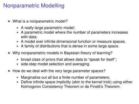
Nonparametric Modelling
I What is a nonparametric model?
I A really large parametric model;I A parametric model where the number of parameters increases
with data;I A model over infinite dimensional function or measure spaces.I A family of distributions that is dense in some large space.
I Why nonparametric models in Bayesian theory of learning?
I broad class of priors that allows data to “speak for itself”;I side-step model selection and averaging.
I How do we deal with the very large parameter spaces?
I Marginalize out all but a finite number of parameters;I Define infinite space implicitly (akin to the kernel trick) using either
Kolmogorov Consistency Theorem or de Finetti’s Theorem.
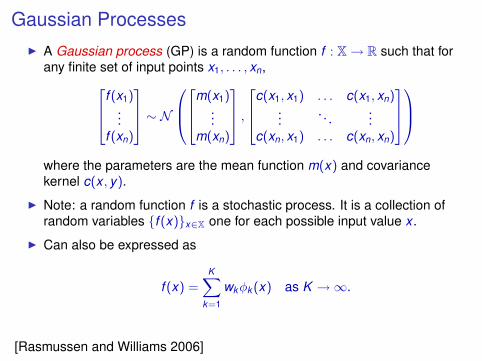
Gaussian ProcessesI A Gaussian process (GP) is a random function f : X→ R such that for
any finite set of input points x1, . . . , xn,f (x1)...
f (xn)
∼ Nm(x1)
...m(xn)
,c(x1, x1) . . . c(x1, xn)
.... . .
...c(xn, x1) . . . c(xn, xn)
where the parameters are the mean function m(x) and covariancekernel c(x , y).
I Note: a random function f is a stochastic process. It is a collection ofrandom variables {f (x)}x∈X one for each possible input value x .
I Can also be expressed as
f (x) =K∑
k=1
wkφk (x) as K →∞.
[Rasmussen and Williams 2006]
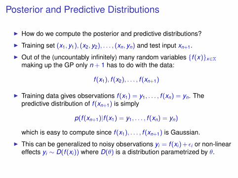
Posterior and Predictive Distributions
I How do we compute the posterior and predictive distributions?
I Training set (x1, y1), (x2, y2), . . . , (xn, yn) and test input xn+1.
I Out of the (uncountably infinitely) many random variables {f (x)}x∈Xmaking up the GP only n + 1 has to do with the data:
f (x1), f (x2), . . . , f (xn+1)
I Training data gives observations f (x1) = y1, . . . , f (xn) = yn. Thepredictive distribution of f (xn+1) is simply
p(f (xn+1)|f (x1) = y1, . . . , f (xn) = yn)
which is easy to compute since f (x1), . . . , f (xn+1) is Gaussian.
I This can be generalized to noisy observations yi = f (xi ) + εi or non-lineareffects yi ∼ D(f (xi )) where D(θ) is a distribution parametrized by θ.
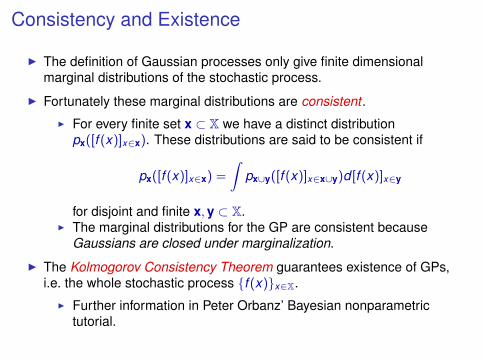
Consistency and Existence
I The definition of Gaussian processes only give finite dimensionalmarginal distributions of the stochastic process.
I Fortunately these marginal distributions are consistent .
I For every finite set x ⊂ X we have a distinct distributionpx([f (x)]x∈x). These distributions are said to be consistent if
px([f (x)]x∈x) =
∫px∪y([f (x)]x∈x∪y)d [f (x)]x∈y
for disjoint and finite x,y ⊂ X.I The marginal distributions for the GP are consistent because
Gaussians are closed under marginalization.
I The Kolmogorov Consistency Theorem guarantees existence of GPs,i.e. the whole stochastic process {f (x)}x∈X.
I Further information in Peter Orbanz’ Bayesian nonparametrictutorial.
Outline
Some Examples of Parametric Models
Bayesian Nonparametric Modelling
Infinite Mixture Models
Some Measure Theory
Dirichlet Processes
Indian Buffet and Beta Processes
Hierarchical Dirichlet Processes
Pitman-Yor Processes
Summary
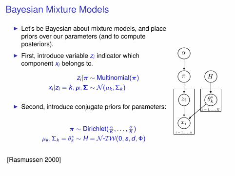
Bayesian Mixture Models
I Let’s be Bayesian about mixture models, and placepriors over our parameters (and to computeposteriors).
I First, introduce variable zi indicator whichcomponent xi belongs to.
zi |π ∼ Multinomial(π)
xi |zi = k ,µ,Σ ∼ N (µk ,Σk )
I Second, introduce conjugate priors for parameters:
π ∼ Dirichlet(αK , . . . ,αK )
µk ,Σk = θ∗k ∼ H = N -IW(0, s,d ,Φ)
[Rasmussen 2000]
zi
π
α
H
i = 1, . . . , n
xi
θ∗kk = 1, . . . ,K
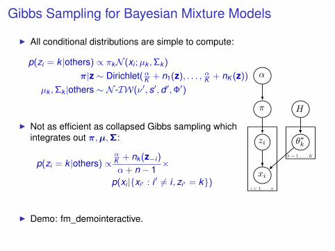
Gibbs Sampling for Bayesian Mixture Models
I All conditional distributions are simple to compute:
p(zi = k |others) ∝ πkN (xi ;µk ,Σk )
π|z ∼ Dirichlet(αK + n1(z), . . . , αK + nK (z))
µk ,Σk |others ∼ N -IW(ν′, s′,d ′,Φ′)
I Not as efficient as collapsed Gibbs sampling whichintegrates out π,µ,Σ:
p(zi = k |others) ∝αK + nk (z−i )
α + n − 1×
p(xi |{xi′ : i ′ 6= i , zi′ = k})
I Demo: fm_demointeractive.
zi
π
α
H
i = 1, . . . , n
xi
θ∗kk = 1, . . . ,K
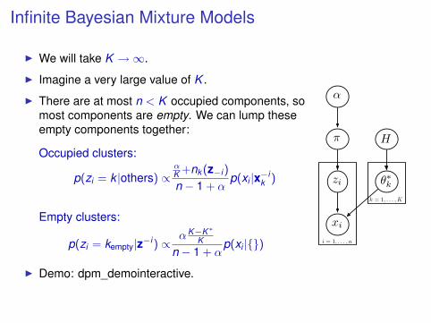
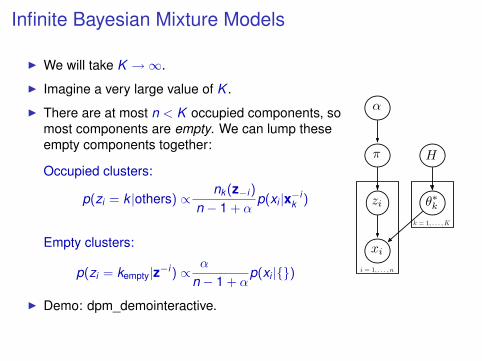
Infinite Bayesian Mixture Models
I We will take K →∞.
I Imagine a very large value of K .
I There are at most n < K occupied components, somost components are empty. We can lump theseempty components together:
Occupied clusters:
p(zi = k |others) ∝αK +nk (z−i )
n − 1 + αp(xi |x−i
k )
Empty clusters:
p(zi = kempty|z−i ) ∝ αK−K∗K
n − 1 + αp(xi |{})
I Demo: dpm_demointeractive.
zi
π
α
H
i = 1, . . . , n
xi
θ∗kk = 1, . . . ,K
Infinite Bayesian Mixture Models
I The actual infinite limit of finite mixture models does not make sense:any particular component will get a mixing proportion of 0.
I In the Gibbs sampler we bypassed this by lumping empty clusterstogether.
I Other better ways of making this infinite limit precise:
I Look at the prior clustering structure induced by the Dirichlet priorover mixing proportions—Chinese restaurant process.
I Re-order components so that those with larger mixing proportionstend to occur first, before taking the infinite limit—stick-breakingconstruction.
I Both are different views of the Dirichlet process (DP).
I DPs can be thought of as infinite dimensional Dirichlet distributions.
I The K →∞ Gibbs sampler is for DP mixture models.
Outline
Some Examples of Parametric Models
Bayesian Nonparametric Modelling
Infinite Mixture Models
Some Measure Theory
Dirichlet Processes
Indian Buffet and Beta Processes
Hierarchical Dirichlet Processes
Pitman-Yor Processes
Summary

A Tiny Bit of Measure Theoretic Probability Theory
I A σ-algebra Σ is a family of subsets of a set Θ such that
I Σ is not empty;I If A ∈ Σ then Θ\A ∈ Σ;I If A1,A2, . . . ∈ Σ then ∪∞i=1Ai ∈ Σ.
I (Θ,Σ) is a measure space and A ∈ Σ are the measurable sets.
I A measure µ over (Θ,Σ) is a function µ : Σ→ [0,∞] such that
I µ(∅) = 0;I If A1,A2, . . . ∈ Σ are disjoint then µ(∪∞i=1Ai ) =
∑∞i=1 µ(Ai ).
I Everything we consider here will be measurable.I A probability measure is one where µ(Θ) = 1.
I Given two measure spaces (Θ,Σ) and (∆,Φ), a function f : Θ→ ∆ ismeasurable if f−1(A) ∈ Σ for every A ∈ Φ.
A Tiny Bit of Measure Theoretic Probability Theory
I If p is a probability measure on (Θ,Σ), a random variable X takingvalues in ∆ is simply a measurable function X : Θ→ ∆.
I Think of the probability space (Θ,Σ,p) as a black-box randomnumber generator, and X as a function taking random samples in Θand producing random samples in ∆.
I The probability of an event A ∈ Φ is p(X ∈ A) = p(X−1(A)).
I A stochastic process is simply a collection of random variables {Xi}i∈Iover the same measure space (Θ,Σ), where I is an index set.
I What distinguishes a stochastic process from, say, a graphicalmodel is that I can be infinite, even uncountably so.
I This raises issues of how do you even define them and how do youensure that they can even existence (mathematically speaking).
I Stochastic processes form the core of many Bayesian nonparametricmodels.
I Gaussian processes, Poisson processes, gamma processes,Dirichlet processes, beta processes...
Outline
Some Examples of Parametric Models
Bayesian Nonparametric Modelling
Infinite Mixture Models
Some Measure Theory
Dirichlet Processes
Indian Buffet and Beta Processes
Hierarchical Dirichlet Processes
Pitman-Yor Processes
Summary

Dirichlet Distributions
I A Dirichlet distribution is a distribution over the K -dimensional probabilitysimplex:
∆K ={
(π1, . . . , πK ) : πk ≥ 0,∑
k πk = 1}
I We say (π1, . . . , πK ) is Dirichlet distributed,
(π1, . . . , πK ) ∼ Dirichlet(λ1, . . . , λK )
with parameters (λ1, . . . , λK ), if
p(π1, . . . , πK ) =Γ(∑
k λk )∏k Γ(λk )
n∏k=1
πλk−1k
I Equivalent to normalizing a set of independent gamma variables:
(π1, . . . , πK ) = 1Pk γk
(γ1, . . . , γK )
γk ∼ Gamma(λk ) for k = 1, . . . ,K
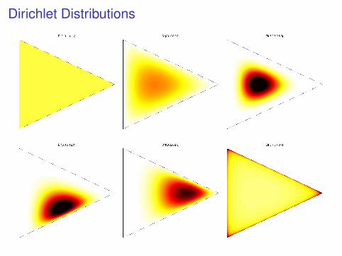
Dirichlet Distributions
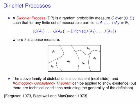
Dirichlet Processes
I A Dirichlet Process (DP) is a random probability measure G over (Θ,Σ)such that for any finite set of measurable partitions A1∪̇ . . . ∪̇AK = Θ,
(G(A1), . . . ,G(AK )) ∼ Dirichlet(λ(A1), . . . , λ(AK ))
where λ is a base measure.
6
A
A1
A A
A
A
2
3
4
5
I The above family of distributions is consistent (next slide), andKolmogorov Consistency Theorem can be applied to show existence (butthere are technical conditions restricting the generality of the definition).
[Ferguson 1973, Blackwell and MacQueen 1973]
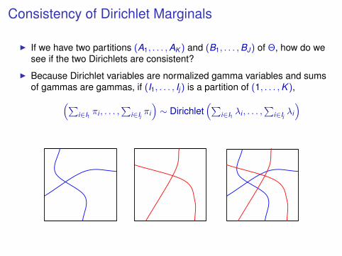
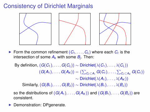
Consistency of Dirichlet Marginals
I If we have two partitions (A1, . . . ,AK ) and (B1, . . . ,BJ) of Θ, how do wesee if the two Dirichlets are consistent?
I Because Dirichlet variables are normalized gamma variables and sumsof gammas are gammas, if (I1, . . . , Ij ) is a partition of (1, . . . ,K ),(∑
i∈I1 πi , . . . ,∑
i∈Ij πi
)∼ Dirichlet
(∑i∈I1 λi , . . . ,
∑i∈Ij λi
)
Consistency of Dirichlet Marginals
I Form the common refinement (C1, . . . ,CL) where each C` is theintersection of some Ak with some Bj . Then:
By definition, (G(C1), . . . ,G(CL)) ∼ Dirichlet(λ(C1), . . . , λ(CL))
(G(A1), . . . ,G(AK )) =(∑
C`⊂A1G(C`), . . . ,
∑C`⊂AK
G(C`))
∼ Dirichlet(λ(A1), . . . , λ(AK ))
Similarly, (G(B1), . . . ,G(BJ)) ∼ Dirichlet(λ(B1), . . . , λ(BJ))
so the distributions of (G(A1), . . . ,G(AK )) and (G(B1), . . . ,G(BJ)) areconsistent.
I Demonstration: DPgenerate.
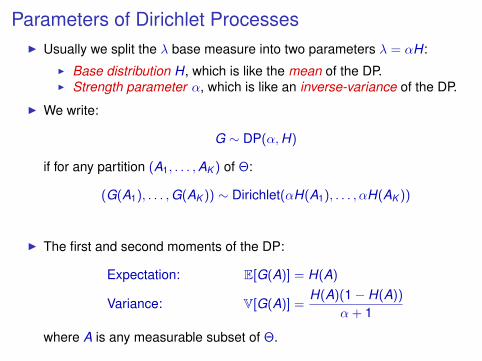
Parameters of Dirichlet ProcessesI Usually we split the λ base measure into two parameters λ = αH:
I Base distribution H, which is like the mean of the DP.I Strength parameter α, which is like an inverse-variance of the DP.
I We write:
G ∼ DP(α,H)
if for any partition (A1, . . . ,AK ) of Θ:
(G(A1), . . . ,G(AK )) ∼ Dirichlet(αH(A1), . . . , αH(AK ))
I The first and second moments of the DP:
Expectation: E[G(A)] = H(A)
Variance: V[G(A)] =H(A)(1− H(A))
α + 1
where A is any measurable subset of Θ.
Representations of Dirichlet ProcessesI Draws from Dirichlet processes will always place all their mass on a
countable set of points:
G =∞∑
k=1
πkδθ∗k
where∑
k πk = 1 and θ∗k ∈ Θ.I What is the joint distribution over π1, π2, . . . and θ∗1 , θ
∗2 , . . .?
I Since G is a (random) probability measure over Θ, we can treat it as adistribution and draw samples from it. Let
θ1, θ2, . . . ∼ G
be random variables with distribution G.I What is the marginal distribution of θ1, θ2, . . . with G integrated out?I There is positive probability that sets of θi ’s can take on the same
value θ∗k for some k , i.e. the θi ’s cluster together. How do theseclusters look like?
I For practical modelling purposes this is sufficient. But is thissufficient to tell us all about G?
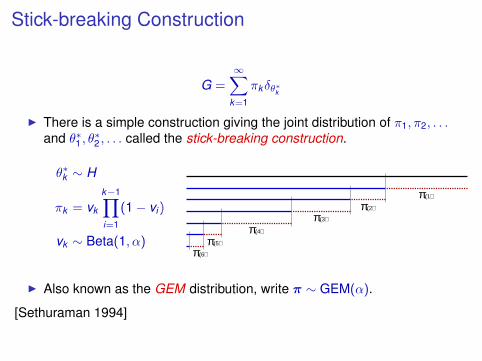
Stick-breaking Construction
G =∞∑
k=1
πkδθ∗k
I There is a simple construction giving the joint distribution of π1, π2, . . .and θ∗1 , θ
∗2 , . . . called the stick-breaking construction.
θ∗k ∼ H
πk = vk
k−1∏i=1
(1− vi )
vk ∼ Beta(1, α)
π
(4)π(5)π
(2)π(3)π
(6)π
(1)
I Also known as the GEM distribution, write π ∼ GEM(α).
[Sethuraman 1994]
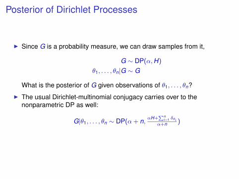
Posterior of Dirichlet Processes
I Since G is a probability measure, we can draw samples from it,
G ∼ DP(α,H)
θ1, . . . , θn|G ∼ G
What is the posterior of G given observations of θ1, . . . , θn?
I The usual Dirichlet-multinomial conjugacy carries over to thenonparametric DP as well:
G|θ1, . . . , θn ∼ DP(α + n, αH+Pn
i=1 δθiα+n )
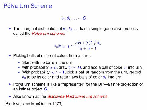
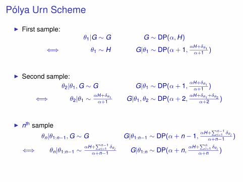
Pólya Urn Scheme
θ1, θ2, . . . ∼ G
I The marginal distribution of θ1, θ2, . . . has a simple generative processcalled the Pólya urn scheme.
θn|θ1:n−1 ∼ αH +∑n−1
i=1 δθi
α + n − 1
I Picking balls of different colors from an urn:
I Start with no balls in the urn.I with probability ∝ α, draw θn ∼ H, and add a ball of color θn into urn.I With probability ∝ n − 1, pick a ball at random from the urn, recordθn to be its color and return two balls of color θn into urn.
I Pólya urn scheme is like a “representer” for the DP—a finite projection ofan infinite object G.
I Also known as the Blackwell-MacQueen urn scheme.
[Blackwell and MacQueen 1973]
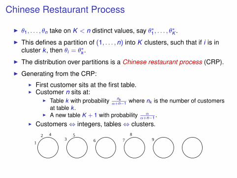
Chinese Restaurant Process
I θ1, . . . , θn take on K < n distinct values, say θ∗1 , . . . , θ∗K .
I This defines a partition of (1, . . . ,n) into K clusters, such that if i is incluster k , then θi = θ∗k .
I The distribution over partitions is a Chinese restaurant process (CRP).
I Generating from the CRP:
I First customer sits at the first table.I Customer n sits at:
I Table k with probability nkα+n−1 where nk is the number of customers
at table k .I A new table K + 1 with probability α
α+n−1 .I Customers⇔ integers, tables⇔ clusters.
91
23
4 56 7
8
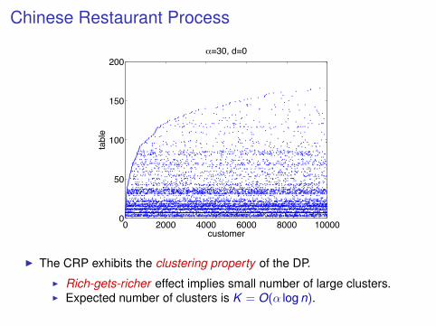
Chinese Restaurant Process
0 2000 4000 6000 8000 100000
50
100
150
200
customer
tabl
e
!=30, d=0
I The CRP exhibits the clustering property of the DP.
I Rich-gets-richer effect implies small number of large clusters.I Expected number of clusters is K = O(α log n).
Exchangeability
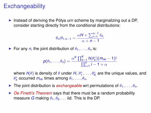
I Instead of deriving the Pólya urn scheme by marginalizing out a DP,consider starting directly from the conditional distributions:
θn|θ1:n−1 ∼ αH +∑n−1
i=1 δθi
α + n − 1
I For any n, the joint distribution of θ1, . . . , θn is:
p(θ1, . . . , θn) =αK ∏K
k=1 h(θ∗k )(mnk − 1)!∏ni=1 i − 1 + α
where h(θ) is density of θ under H, θ∗1 , . . . , θ∗K are the unique values, and
θ∗k occurred mnk times among θ1, . . . , θn.
I The joint distribution is exchangeable wrt permutations of θ1, . . . , θn.
I De Finetti’s Theorem says that there must be a random probabilitymeasure G making θ1, θ2, . . . iid. This is the DP.
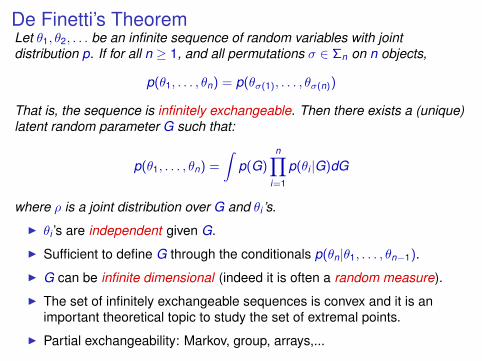
De Finetti’s TheoremLet θ1, θ2, . . . be an infinite sequence of random variables with jointdistribution p. If for all n ≥ 1, and all permutations σ ∈ Σn on n objects,
p(θ1, . . . , θn) = p(θσ(1), . . . , θσ(n))
That is, the sequence is infinitely exchangeable. Then there exists a (unique)latent random parameter G such that:
p(θ1, . . . , θn) =
∫p(G)
n∏i=1
p(θi |G)dG
where ρ is a joint distribution over G and θi ’s.
I θi ’s are independent given G.
I Sufficient to define G through the conditionals p(θn|θ1, . . . , θn−1).
I G can be infinite dimensional (indeed it is often a random measure).
I The set of infinitely exchangeable sequences is convex and it is animportant theoretical topic to study the set of extremal points.
I Partial exchangeability: Markov, group, arrays,...
Outline
Some Examples of Parametric Models
Bayesian Nonparametric Modelling
Infinite Mixture Models
Some Measure Theory
Dirichlet Processes
Indian Buffet and Beta Processes
Hierarchical Dirichlet Processes
Pitman-Yor Processes
Summary
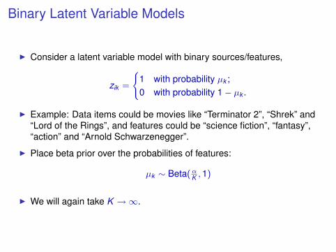
Binary Latent Variable Models
I Consider a latent variable model with binary sources/features,
zik =
{1 with probability µk ;0 with probability 1− µk .
I Example: Data items could be movies like “Terminator 2”, “Shrek” and“Lord of the Rings”, and features could be “science fiction”, “fantasy”,“action” and “Arnold Schwarzenegger”.
I Place beta prior over the probabilities of features:
µk ∼ Beta(αK ,1)
I We will again take K →∞.
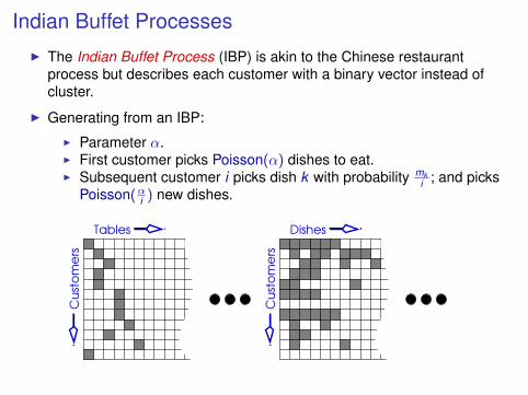
Indian Buffet ProcessesI The Indian Buffet Process (IBP) is akin to the Chinese restaurant
process but describes each customer with a binary vector instead ofcluster.
I Generating from an IBP:
I Parameter α.I First customer picks Poisson(α) dishes to eat.I Subsequent customer i picks dish k with probability mk
i ; and picksPoisson(αi ) new dishes.
Tables
Cu
sto
me
rs
Dishes
Cu
sto
me
rs
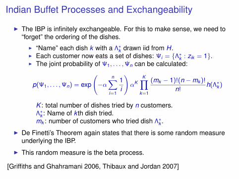
Indian Buffet Processes and Exchangeability
I The IBP is infinitely exchangeable. For this to make sense, we need to“forget” the ordering of the dishes.
I “Name” each dish k with a Λ∗k drawn iid from H.I Each customer now eats a set of dishes: Ψi = {Λ∗k : zik = 1}.I The joint probability of Ψ1, . . . ,Ψn can be calculated:
p(Ψ1, . . . ,Ψn) = exp
(−α
n∑i=1
1i
)αK
K∏k=1
(mk − 1)!(n −mk )!
n!h(Λ∗k )
K : total number of dishes tried by n customers.Λ∗k : Name of k th dish tried.mk : number of customers who tried dish Λ∗k .
I De Finetti’s Theorem again states that there is some random measureunderlying the IBP.
I This random measure is the beta process.
[Griffiths and Ghahramani 2006, Thibaux and Jordan 2007]
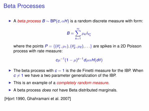
Beta Processes
I A beta process B ∼ BP(c, αH) is a random discrete measure with form:
B =∞∑
k=1
µkδθ∗k
where the points P = {(θ∗1 , µ1), (θ∗2 , µ2), . . .} are spikes in a 2D Poissonprocess with rate measure:
cµ−1(1− µ)c−1dµαH(dθ)
I The beta process with c = 1 is the de Finetti measure for the IBP. Whenc 6= 1 we have a two parameter generalization of the IBP.
I This is an example of a completely random measure.
I A beta process does not have Beta distributed marginals.
[Hjort 1990, Ghahramani et al. 2007]
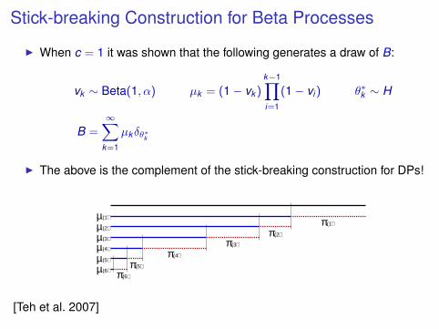
Stick-breaking Construction for Beta Processes
I When c = 1 it was shown that the following generates a draw of B:
vk ∼ Beta(1, α) µk = (1− vk )k−1∏i=1
(1− vi ) θ∗k ∼ H
B =∞∑
k=1
µkδθ∗k
I The above is the complement of the stick-breaking construction for DPs!
π
(4)π(3)µ
(6)µ
(1)µ(2)µ
(4)µ(5)µ
(5)π
(2)π(3)π
(6)π
(1)
[Teh et al. 2007]
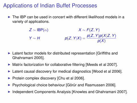
Applications of Indian Buffet Processes
I The IBP can be used in concert with different likelihood models in avariety of applications.
Z ∼ IBP(α) X ∼ F (Z ,Y )
Y ∼ H p(Z ,Y |X ) =p(Z ,Y )p(X |Z ,Y )
p(X )
I Latent factor models for distributed representation [Griffiths andGhahramani 2005].
I Matrix factorization for collaborative filtering [Meeds et al 2007].
I Latent causal discovery for medical diagnostics [Wood et al 2006].
I Protein complex discovery [Chu et al 2006].
I Psychological choice behaviour [Görür and Rasmussen 2006].
I Independent Components Analysis [Knowles and Ghahramani 2007].
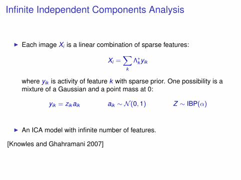
Infinite Independent Components Analysis
I Each image Xi is a linear combination of sparse features:
Xi =∑
k
Λ∗k yik
where yik is activity of feature k with sparse prior. One possibility is amixture of a Gaussian and a point mass at 0:
yik = zik aik aik ∼ N (0,1) Z ∼ IBP(α)
I An ICA model with infinite number of features.
[Knowles and Ghahramani 2007]
Outline
Some Examples of Parametric Models
Bayesian Nonparametric Modelling
Infinite Mixture Models
Some Measure Theory
Dirichlet Processes
Indian Buffet and Beta Processes
Hierarchical Dirichlet Processes
Pitman-Yor Processes
Summary
Topic Modelling with Latent Dirichlet Allocation
I Infer topics from a document corpus, topicsbeing sets of words that tend to co-occurtogether.
I Using (Bayesian) latent Dirichlet allocation:
πj ∼ Dirichlet(αK , . . . ,αK )
θk ∼ Dirichlet( βW , . . . , βW )
zji |πj ∼ Multinomial(πj )
xji |zji ,θzji ∼ Multinomial(θzji )
I Can we take K →∞?
topics k=1...K
document j=1...D
words i=1...nd
πj
zji
xji θk
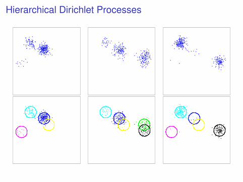
Hierarchical Dirichlet Processes
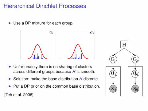
Hierarchical Dirichlet Processes
I Use a DP mixture for each group.
I Unfortunately there is no sharing of clustersacross different groups because H is smooth.
I Solution: make the base distribution H discrete.
I Put a DP prior on the common base distribution.
[Teh et al. 2006]
H
1i
1ix
θ
G1 G
x
θ
2
2i
2i
Hierarchical Dirichlet Processes
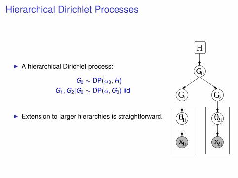
I A hierarchical Dirichlet process:
G0 ∼ DP(α0,H)
G1,G2|G0 ∼ DP(α,G0) iid
I Extension to larger hierarchies is straightforward. 1i
1ix
θ
G1 G
x
θ
G
H
0
2
2i
2i
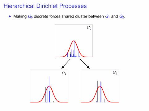
Hierarchical Dirichlet Processes
I Making G0 discrete forces shared cluster between G1 and G2.
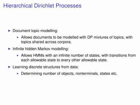
Hierarchical Dirichlet Processes
I Document topic modelling:
I Allows documents to be modelled with DP mixtures of topics, withtopics shared across corpora.
I Infinite hidden Markov modelling:
I Allows HMMs with an infinite number of states, with transitions fromeach allowable state to every other allowable state.
I Learning discrete structures from data:
I Determining number of objects, nonterminals, states etc.
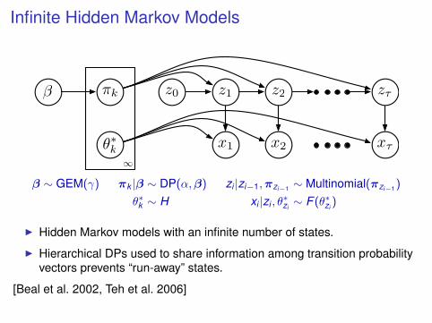
Infinite Hidden Markov Models
z0 z1 z2 zτ
x1 x2 xτ
β πk
θ∗k∞
β ∼ GEM(γ) πk |β ∼ DP(α,β) zi |zi−1,πzi−1 ∼ Multinomial(πzi−1 )
θ∗k ∼ H xi |zi , θ∗zi∼ F (θ∗zi
)
I Hidden Markov models with an infinite number of states.
I Hierarchical DPs used to share information among transition probabilityvectors prevents “run-away” states.
[Beal et al. 2002, Teh et al. 2006]
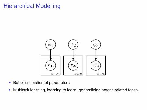
Hierarchical Modelling
i=1...n2
φ2
x2i
i=1...n3
φ3
x3i
i=1...n1
φ1
x1i
I Better estimation of parameters.
I Multitask learning, learning to learn: generalizing across related tasks.
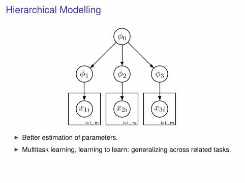
Hierarchical Modelling
i=1...n2
φ0
φ2
x2i
i=1...n3
φ3
x3i
i=1...n1
φ1
x1i
I Better estimation of parameters.
I Multitask learning, learning to learn: generalizing across related tasks.
Outline
Some Examples of Parametric Models
Bayesian Nonparametric Modelling
Infinite Mixture Models
Some Measure Theory
Dirichlet Processes
Indian Buffet and Beta Processes
Hierarchical Dirichlet Processes
Pitman-Yor Processes
Summary
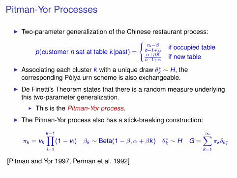
Pitman-Yor Processes
I Two-parameter generalization of the Chinese restaurant process:
p(customer n sat at table k |past) =
{nk−β
n−1+α if occupied tableα+βKn−1+α if new table
I Associating each cluster k with a unique draw θ∗k ∼ H, thecorresponding Pólya urn scheme is also exchangeable.
I De Finetti’s Theorem states that there is a random measure underlyingthis two-parameter generalization.
I This is the Pitman-Yor process.
I The Pitman-Yor process also has a stick-breaking construction:
πk = vk
k−1∏i=1
(1− vi ) βk ∼ Beta(1− β, α + βk) θ∗k ∼ H G =∞∑
k=1
πkδθ∗k
[Pitman and Yor 1997, Perman et al. 1992]
Pitman-Yor Processes
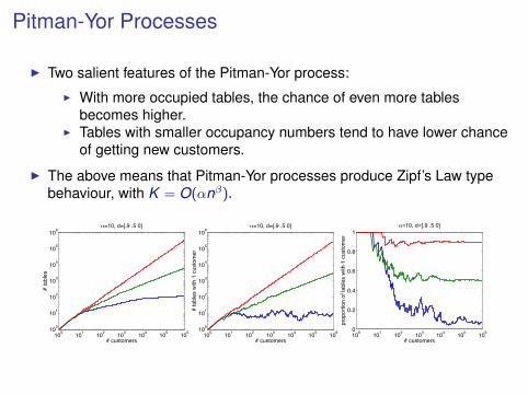
I Two salient features of the Pitman-Yor process:
I With more occupied tables, the chance of even more tablesbecomes higher.
I Tables with smaller occupancy numbers tend to have lower chanceof getting new customers.
I The above means that Pitman-Yor processes produce Zipf’s Law typebehaviour, with K = O(αnβ).
100 101 102 103 104 105 106100
101
102
103
104
105
106
# customers
# ta
bles
!=10, d=[.9 .5 0]
100 101 102 103 104 105 106100
101
102
103
104
105
106
# customers
# ta
bles
with
1 c
usto
mer
!=10, d=[.9 .5 0]
100 101 102 103 104 105 1060
0.2
0.4
0.6
0.8
1
# customerspr
opor
tion
of ta
bles
with
1 c
usto
mer
!=10, d=[.9 .5 0]
Pitman-Yor Processes
Draw from a Pitman-Yor process
0 2000 4000 6000 8000 100000
50
100
150
200
250
customer
tabl
e
!=1, d=.5
0 200 400 600 800100
101
102
103
104
105
# tables#
cust
omer
s pe
r tab
le
!=1, d=.5
100 101 102 103100
101
102
103
104
105
# tables
# cu
stom
ers
per t
able
!=1, d=.5
Draw from a Dirichlet process
0 2000 4000 6000 8000 100000
50
100
150
200
customer
tabl
e
!=30, d=0
0 50 100 150 200 250100
101
102
103
104
105
# tables
# cu
stom
ers
per t
able
!=30, d=0
100 101 102 103100
101
102
103
104
105
# tables#
cust
omer
s pe
r tab
le
!=30, d=0
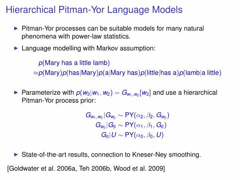
Hierarchical Pitman-Yor Language Models
I Pitman-Yor processes can be suitable models for many naturalphenomena with power-law statistics.
I Language modelling with Markov assumption:
p(Mary has a little lamb)
≈p(Mary)p(has|Mary)p(a|Mary has)p(little|has a)p(lamb|a little)
I Parameterize with p(w3|w1,w2) = Gw1,w2 [w3] and use a hierarchicalPitman-Yor process prior:
Gw1,w2 |Gw2 ∼ PY(α2, β2,Gw2 )
Gw2 |G∅ ∼ PY(α1, β1,G∅)G∅|U ∼ PY(α0, β0,U)
I State-of-the-art results, connection to Kneser-Ney smoothing.
[Goldwater et al. 2006a, Teh 2006b, Wood et al. 2009]
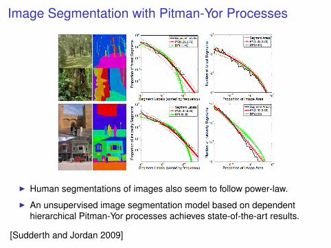
Image Segmentation with Pitman-Yor Processes
I Human segmentations of images also seem to follow power-law.
I An unsupervised image segmentation model based on dependenthierarchical Pitman-Yor processes achieves state-of-the-art results.
[Sudderth and Jordan 2009]
Outline
Some Examples of Parametric Models
Bayesian Nonparametric Modelling
Infinite Mixture Models
Some Measure Theory
Dirichlet Processes
Indian Buffet and Beta Processes
Hierarchical Dirichlet Processes
Pitman-Yor Processes
Summary
SummaryI Motivation for Bayesian nonparametrics:
I Allows practitioners to define and work with models with largesupport, sidesteps model selection.
I New models with useful properties.I Large variety of applications.
I Various standard Bayesian nonparametric models:I Dirichlet processesI Hierarchical Dirichlet processesI Infinite hidden Markov modelsI Indian buffet and beta processesI Pitman-Yor processes
I Touched upon two important theoretical tools:I Consistency and Kolmogorov’s Consistency TheoremI Exchangeability and de Finetti’s Theorem
I Described a number of applications of Bayesian nonparametrics.
I Missing: Inference methods based on MCMC, variational etc,consistency and convergence.
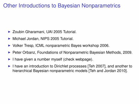
Other Introductions to Bayesian Nonparametrics
I Zoubin Gharamani, UAI 2005 Tutorial.
I Michael Jordan, NIPS 2005 Tutorial.
I Volker Tresp, ICML nonparametric Bayes workshop 2006.
I Peter Orbanz, Foundations of Nonparametric Bayesian Methods, 2009.
I I have given a number myself (check webpage).
I I have an introduction to Dirichlet processes [Teh 2007], and another tohierarchical Bayesian nonparametric models [Teh and Jordan 2010].
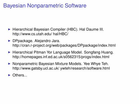
Bayesian Nonparametric Software
I Hierarchical Bayesian Compiler (HBC). Hal Daume III.http://www.cs.utah.edu/ hal/HBC/
I DPpackage. Alejandro Jara.http://cran.r-project.org/web/packages/DPpackage/index.html
I Hierarchical Pitman Yor Language Model. Songfang Huang.http://homepages.inf.ed.ac.uk/s0562315/progs/index.html
I Nonparametric Bayesian Mixture Models. Yee Whye Teh.http://www.gatsby.ucl.ac.uk/ ywteh/research/software.html
I Others...

AISTATS 2010
May 13-15, 2010. Chia Laguna Resort, Sardinia, Italy
http://www.aistats.org
Deadline: November 6, 2009
Outline
Relating Different Representations of Dirichlet Processes
Representations of Hierarchical Dirichlet Processes
Extended Bibliography
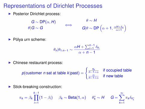
Representations of Dirichlet ProcessesI Posterior Dirichlet process:
G ∼ DP(α,H)
θ|G ∼ G⇐⇒
θ ∼ H
G|θ ∼ DP(α + 1, αH+δθ
α+1
)I Pólya urn scheme:
θn|θ1:n−1 ∼ αH +∑n−1
i=1 δθi
α + n − 1
I Chinese restaurant process:
p(customer n sat at table k |past) =
{nk
n−1+α if occupied tableα
n−1+α if new table
I Stick-breaking construction:
πk = βk
k−1∏i=1
(1− βi ) βk ∼ Beta(1, α) θ∗k ∼ H G =∞∑
k=1
πkδθ∗k
Posterior Dirichlet Processes
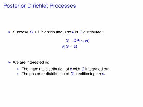
I Suppose G is DP distributed, and θ is G distributed:
G ∼ DP(α,H)
θ|G ∼ G
I We are interested in:
I The marginal distribution of θ with G integrated out.I The posterior distribution of G conditioning on θ.
Posterior Dirichlet Processes
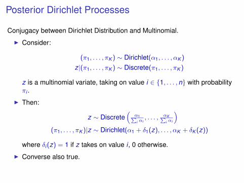
Conjugacy between Dirichlet Distribution and Multinomial.
I Consider:
(π1, . . . , πK ) ∼ Dirichlet(α1, . . . , αK )
z|(π1, . . . , πK ) ∼ Discrete(π1, . . . , πK )
z is a multinomial variate, taking on value i ∈ {1, . . . ,n} with probabilityπi .
I Then:
z ∼ Discrete(
α1Pi αi, . . . , αKP
i αi
)(π1, . . . , πK )|z ∼ Dirichlet(α1 + δ1(z), . . . , αK + δK (z))
where δi (z) = 1 if z takes on value i , 0 otherwise.
I Converse also true.
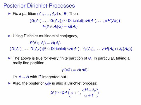
Posterior Dirichlet ProcessesI Fix a partition (A1, . . . ,AK ) of Θ. Then
(G(A1), . . . ,G(AK )) ∼ Dirichlet(αH(A1), . . . , αH(AK ))
P(θ ∈ Ai |G) = G(Ai )
I Using Dirichlet-multinomial conjugacy,
P(θ ∈ Ai ) = H(Ai )
(G(A1), . . . ,G(AK ))|θ ∼ Dirichlet(αH(A1)+δθ(A1), . . . , αH(AK )+δθ(AK ))
I The above is true for every finite partition of Θ. In particular, taking areally fine partition,
p(dθ) = H(dθ)
i.e. θ ∼ H with G integrated out.I Also, the posterior G|θ is also a Dirichlet process:
G|θ ∼ DP(α + 1,
αH + δθα + 1
)
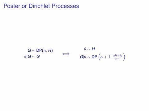
Posterior Dirichlet Processes
G ∼ DP(α,H)
θ|G ∼ G⇐⇒
θ ∼ H
G|θ ∼ DP(α + 1, αH+δθ
α+1
)
Pólya Urn Scheme
I First sample:θ1|G ∼ G G ∼ DP(α,H)
⇐⇒ θ1 ∼ H G|θ1 ∼ DP(α + 1, αH+δθ1α+1 )
I Second sample:θ2|θ1,G ∼ G G|θ1 ∼ DP(α + 1, αH+δθ1
α+1 )
⇐⇒ θ2|θ1 ∼ αH+δθ1α+1 G|θ1, θ2 ∼ DP(α + 2, αH+δθ1 +δθ2
α+2 )
I nth sample
θn|θ1:n−1,G ∼ G G|θ1:n−1 ∼ DP(α + n − 1, αH+Pn−1
i=1 δθiα+n−1 )
⇐⇒ θn|θ1:n−1 ∼ αH+Pn−1
i=1 δθiα+n−1 G|θ1:n ∼ DP(α + n, αH+
Pni=1 δθi
α+n )
Stick-breaking ConstructionI Returning to the posterior process:
G ∼ DP(α,H)
θ|G ∼ G⇔
θ ∼ H
G|θ ∼ DP(α + 1, αH+δθα+1 )
I Consider a partition (θ,Θ\θ) of Θ. We have:
(G(θ),G(Θ\θ))|θ ∼ Dirichlet((α + 1)αH+δθα+1 (θ), (α + 1)αH+δθ
α+1 (Θ\θ))
= Dirichlet(1, α)
I G has a point mass located at θ:
G = βδθ + (1− β)G′ with β ∼ Beta(1, α)
and G′ is the (renormalized) probability measure with the point massremoved.
I What is G′?
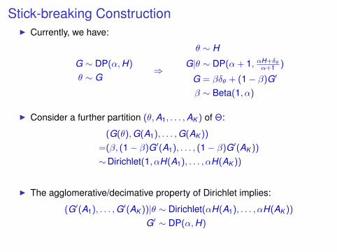
Stick-breaking ConstructionI Currently, we have:
G ∼ DP(α,H)
θ ∼ G⇒
θ ∼ H
G|θ ∼ DP(α + 1, αH+δθα+1 )
G = βδθ + (1− β)G′
β ∼ Beta(1, α)
I Consider a further partition (θ,A1, . . . ,AK ) of Θ:
(G(θ),G(A1), . . . ,G(AK ))
=(β, (1− β)G′(A1), . . . , (1− β)G′(AK ))
∼Dirichlet(1, αH(A1), . . . , αH(AK ))
I The agglomerative/decimative property of Dirichlet implies:
(G′(A1), . . . ,G′(AK ))|θ ∼ Dirichlet(αH(A1), . . . , αH(AK ))
G′ ∼ DP(α,H)
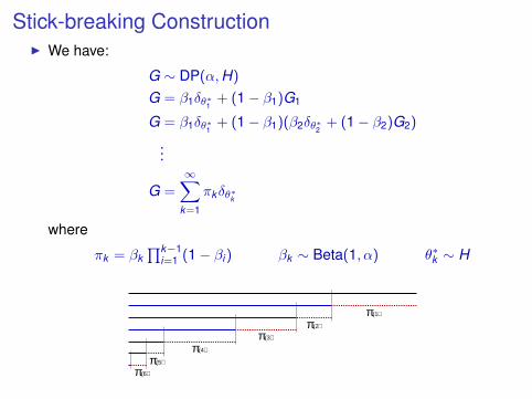
Stick-breaking ConstructionI We have:
G ∼ DP(α,H)
G = β1δθ∗1 + (1− β1)G1
G = β1δθ∗1 + (1− β1)(β2δθ∗2 + (1− β2)G2)
...
G =∞∑
k=1
πkδθ∗k
where
πk = βk∏k−1
i=1 (1− βi ) βk ∼ Beta(1, α) θ∗k ∼ H
π
(4)π(5)π
(2)π(3)π
(6)π
(1)
Outline
Relating Different Representations of Dirichlet Processes
Representations of Hierarchical Dirichlet Processes
Extended Bibliography
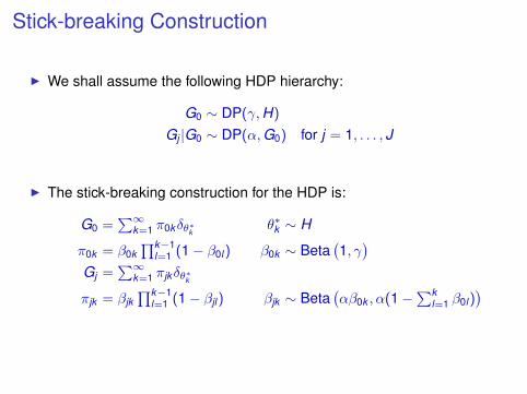
Stick-breaking Construction
I We shall assume the following HDP hierarchy:
G0 ∼ DP(γ,H)
Gj |G0 ∼ DP(α,G0) for j = 1, . . . , J
I The stick-breaking construction for the HDP is:
G0 =∑∞
k=1 π0kδθ∗k θ∗k ∼ H
π0k = β0k∏k−1
l=1 (1− β0l ) β0k ∼ Beta(1, γ)
Gj =∑∞
k=1 πjkδθ∗k
πjk = βjk∏k−1
l=1 (1− βjl ) βjk ∼ Beta(αβ0k , α(1−∑k
l=1 β0l ))
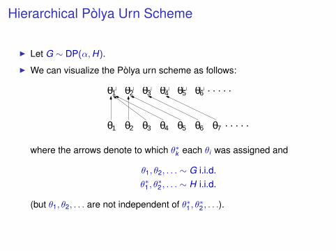
Hierarchical Pòlya Urn Scheme
I Let G ∼ DP(α,H).
I We can visualize the Pòlya urn scheme as follows:
2
1θ θ θ θ θ θ
θ∗θ∗θ∗θ∗θ∗1θ∗ . . . . .
. . . . .θ2 3 4 5 6 7
6543
where the arrows denote to which θ∗k each θi was assigned and
θ1, θ2, . . . ∼ G i.i.d.θ∗1 , θ
∗2 , . . . ∼ H i.i.d.
(but θ1, θ2, . . . are not independent of θ∗1 , θ∗2 , . . .).
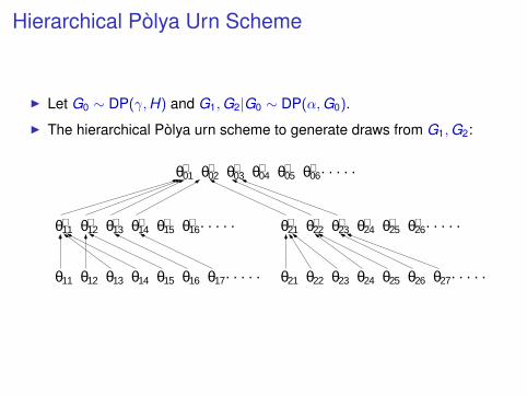
Hierarchical Pòlya Urn Scheme
I Let G0 ∼ DP(γ,H) and G1,G2|G0 ∼ DP(α,G0).
I The hierarchical Pòlya urn scheme to generate draws from G1,G2:
21θ θ θ θ θ
θ∗θ∗θ∗θ∗θ∗θ∗ . . . . .
. . . . .θ
11 12 13 14 15 16
11 12 13 14 15 θ16 17
θ∗θ∗θ∗θ∗θ∗θ∗ . . . . .21 22 23 24 25 26
θ∗θ∗θ∗θ∗θ∗θ∗ . . . . .01 02 03 0504 06
θ θ θ θ . . . . .θ θ θ272625242322
Chinese Restaurant Franchise
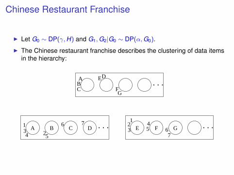
I Let G0 ∼ DP(γ,H) and G1,G2|G0 ∼ DP(α,G0).
I The Chinese restaurant franchise describes the clustering of data itemsin the hierarchy:
E
. . .134
6 7
52
. . .
. . .7
64
12
53 E F GA B C D
ABC
GF
D
Outline
Relating Different Representations of Dirichlet Processes
Representations of Hierarchical Dirichlet Processes
Extended Bibliography
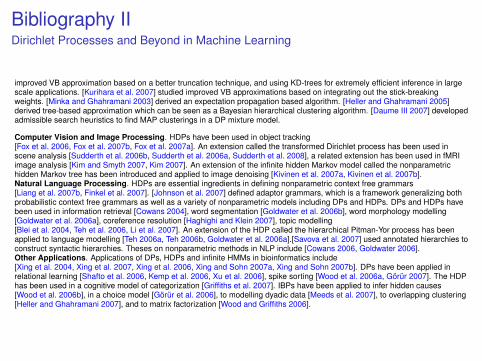
Bibliography IDirichlet Processes and Beyond in Machine LearningDirichlet Processes were first introduced by [Ferguson 1973], while [Antoniak 1974] further developed DPs as well as introducethe mixture of DPs. [Blackwell and MacQueen 1973] showed that the Pólya urn scheme is exchangeable with the DP being its deFinetti measure. Further information on the Chinese restaurant process can be obtained at [Aldous 1985, Pitman 2002]. The DPis also related to Ewens’ Sampling Formula [Ewens 1972]. [Sethuraman 1994] gave a constructive definition of the DP via astick-breaking construction. DPs were rediscovered in the machine learning community by [Neal 1992, Rasmussen 2000].
Hierarchical Dirichlet Processes (HDPs) were first developed by [Teh et al. 2006], although an aspect of the model was firstdiscussed in the context of infinite hidden Markov models [Beal et al. 2002]. HDPs and generalizations have been applied acrossa wide variety of fields.Dependent Dirichlet Processes are sets of coupled distributions over probability measures, each of which is marginally DP[MacEachern et al. 2001]. A variety of dependent DPs have been proposed in the literature since then[Srebro and Roweis 2005, Griffin 2007, Caron et al. 2007]. The infinite mixture of Gaussian processes of[Rasmussen and Ghahramani 2002] can also be interpreted as a dependent DP.Indian Buffet Processes (IBPs) were first proposed in [Griffiths and Ghahramani 2006], and extended to a two-parameter familyin [Ghahramani et al. 2007]. [Thibaux and Jordan 2007] showed that the de Finetti measure for the IBP is the beta process of[Hjort 1990], while [Teh et al. 2007] gave a stick-breaking construction and developed efficient slice sampling inference algorithmsfor the IBP.Nonparametric Tree Models are models that use distributions over trees that are consistent and exchangeable. [Blei et al. 2004]used a nested CRP to define distributions over trees with a finite number of levels. [Neal 2001, Neal 2003] defined Dirichletdiffusion trees, which are binary trees produced by a fragmentation process. [Teh et al. 2008] used Kingman’s coalescent[Kingman 1982b, Kingman 1982a] to produce random binary trees using a coalescent process. [Roy et al. 2007] proposedannotated hierarchies, using tree-consistent partitions first defined in [Heller and Ghahramani 2005] to model both relational andfeatural data.
Markov chain Monte Carlo Inference algorithms are the dominant approaches to inference in DP mixtures. [Neal 2000] is agood review of algorithms based on Gibbs sampling in the CRP representation. Algorithm 8 in [Neal 2000] is still one of the bestalgorithms based on simple local moves. [Ishwaran and James 2001] proposed blocked Gibbs sampling in the stick-breakingrepresentation instead due to the simplicity in implementation. This has been further explored in [Porteous et al. 2006]. Sincethen there has been proposals for better MCMC samplers based on proposing larger moves in a Metropolis-Hastings framework[Jain and Neal 2004, Liang et al. 2007a], as well as sequential Monte Carlo [Fearnhead 2004, Mansingkha et al. 2007].Other Approximate Inference Methods have also been proposed for DP mixture models. [Blei and Jordan 2006] is the firstvariational Bayesian approximation, and is based on a truncated stick-breaking representation. [Kurihara et al. 2007] proposed an
Bibliography IIDirichlet Processes and Beyond in Machine Learning
improved VB approximation based on a better truncation technique, and using KD-trees for extremely efficient inference in largescale applications. [Kurihara et al. 2007] studied improved VB approximations based on integrating out the stick-breakingweights. [Minka and Ghahramani 2003] derived an expectation propagation based algorithm. [Heller and Ghahramani 2005]derived tree-based approximation which can be seen as a Bayesian hierarchical clustering algorithm. [Daume III 2007] developedadmissible search heuristics to find MAP clusterings in a DP mixture model.
Computer Vision and Image Processing. HDPs have been used in object tracking[Fox et al. 2006, Fox et al. 2007b, Fox et al. 2007a]. An extension called the transformed Dirichlet process has been used inscene analysis [Sudderth et al. 2006b, Sudderth et al. 2006a, Sudderth et al. 2008], a related extension has been used in fMRIimage analysis [Kim and Smyth 2007, Kim 2007]. An extension of the infinite hidden Markov model called the nonparametrichidden Markov tree has been introduced and applied to image denoising [Kivinen et al. 2007a, Kivinen et al. 2007b].Natural Language Processing. HDPs are essential ingredients in defining nonparametric context free grammars[Liang et al. 2007b, Finkel et al. 2007]. [Johnson et al. 2007] defined adaptor grammars, which is a framework generalizing bothprobabilistic context free grammars as well as a variety of nonparametric models including DPs and HDPs. DPs and HDPs havebeen used in information retrieval [Cowans 2004], word segmentation [Goldwater et al. 2006b], word morphology modelling[Goldwater et al. 2006a], coreference resolution [Haghighi and Klein 2007], topic modelling[Blei et al. 2004, Teh et al. 2006, Li et al. 2007]. An extension of the HDP called the hierarchical Pitman-Yor process has beenapplied to language modelling [Teh 2006a, Teh 2006b, Goldwater et al. 2006a].[Savova et al. 2007] used annotated hierarchies toconstruct syntactic hierarchies. Theses on nonparametric methods in NLP include [Cowans 2006, Goldwater 2006].Other Applications. Applications of DPs, HDPs and infinite HMMs in bioinformatics include[Xing et al. 2004, Xing et al. 2007, Xing et al. 2006, Xing and Sohn 2007a, Xing and Sohn 2007b]. DPs have been applied inrelational learning [Shafto et al. 2006, Kemp et al. 2006, Xu et al. 2006], spike sorting [Wood et al. 2006a, Görür 2007]. The HDPhas been used in a cognitive model of categorization [Griffiths et al. 2007]. IBPs have been applied to infer hidden causes[Wood et al. 2006b], in a choice model [Görür et al. 2006], to modelling dyadic data [Meeds et al. 2007], to overlapping clustering[Heller and Ghahramani 2007], and to matrix factorization [Wood and Griffiths 2006].
References IAldous, D. (1985).Exchangeability and related topics.In École d’Été de Probabilités de Saint-Flour XIII–1983, pages 1–198. Springer, Berlin.
Antoniak, C. E. (1974).Mixtures of Dirichlet processes with applications to Bayesian nonparametric problems.Annals of Statistics, 2(6):1152–1174.
Beal, M. J., Ghahramani, Z., and Rasmussen, C. E. (2002).The infinite hidden Markov model.In Advances in Neural Information Processing Systems, volume 14.
Blackwell, D. and MacQueen, J. B. (1973).Ferguson distributions via Pólya urn schemes.Annals of Statistics, 1:353–355.
Blei, D. M., Griffiths, T. L., Jordan, M. I., and Tenenbaum, J. B. (2004).Hierarchical topic models and the nested Chinese restaurant process.In Advances in Neural Information Processing Systems, volume 16.
Blei, D. M. and Jordan, M. I. (2006).Variational inference for Dirichlet process mixtures.Bayesian Analysis, 1(1):121–144.
Caron, F., Davy, M., and Doucet, A. (2007).Generalized Polya urn for time-varying Dirichlet process mixtures.In Proceedings of the Conference on Uncertainty in Artificial Intelligence, volume 23.
References IICowans, P. (2004).Information retrieval using hierarchical Dirichlet processes.In Proceedings of the Annual International Conference on Research and Development in Information Retrieval,volume 27, pages 564–565.
Cowans, P. (2006).Probabilistic Document Modelling.PhD thesis, University of Cambridge.
Daume III, H. (2007).Fast search for Dirichlet process mixture models.In Proceedings of the International Workshop on Artificial Intelligence and Statistics, volume 11.
Ewens, W. J. (1972).The sampling theory of selectively neutral alleles.Theoretical Population Biology, 3:87–112.
Fearnhead, P. (2004).Particle filters for mixture models with an unknown number of components.Statistics and Computing, 14:11–21.
Ferguson, T. S. (1973).A Bayesian analysis of some nonparametric problems.Annals of Statistics, 1(2):209–230.
Finkel, J. R., Grenager, T., and Manning, C. D. (2007).The infinite tree.In Proceedings of the Annual Meeting of the Association for Computational Linguistics.
References IIIFox, E. B., Choi, D. S., and Willsky, A. S. (2006).Nonparametric Bayesian methods for large scale multi-target tracking.In Proceedings of the Asilomar Conference on Signals, Systems, and Computers, volume 40.
Fox, E. B., Sudderth, E. B., Choi, D. S., and Willsky, A. S. (2007a).Tracking a non-cooperative maneuvering target using hierarchical Dirichlet processes.In Proceedings of the Adaptive Sensor Array Processing Conference.
Fox, E. B., Sudderth, E. B., and Willsky, A. S. (2007b).Hierarchical Dirichlet processes for tracking maneuvering targets.In Proceedings of the International Conference on Information Fusion.
Ghahramani, Z., Griffiths, T. L., and Sollich, P. (2007).Bayesian nonparametric latent feature models (with discussion and rejoinder).In Bayesian Statistics, volume 8.
Goldwater, S. (2006).Nonparametric Bayesian Models of Lexical Acquisition.PhD thesis, Brown University.
Goldwater, S., Griffiths, T., and Johnson, M. (2006a).Interpolating between types and tokens by estimating power-law generators.In Advances in Neural Information Processing Systems, volume 18.
Goldwater, S., Griffiths, T. L., and Johnson, M. (2006b).Contextual dependencies in unsupervised word segmentation.In Proceedings of the 21st International Conference on Computational Linguistics and 44th Annual Meeting of theAssociation for Computational Linguistics.
References IVGörür, D. (2007).Nonparametric Bayesian Discrete Latent Variable Models for Unsupervised Learning.PhD thesis, Technischen Universität Berlin.
Görür, D., Jäkel, F., and Rasmussen, C. E. (2006).A choice model with infinitely many latent features.In Proceedings of the International Conference on Machine Learning, volume 23.
Griffin, J. E. (2007).The Ornstein-Uhlenbeck Dirichlet process and other time-varying processes for Bayesian nonparametric inference.Technical report, Department of Statistics, University of Warwick.
Griffiths, T. L., Canini, K. R., Sanborn, A. N., and Navarro, D. J. (2007).Unifying rational models of categorization via the hierarchical Dirichlet process.In Proceedings of the Annual Conference of the Cognitive Science Society, volume 29.
Griffiths, T. L. and Ghahramani, Z. (2006).Infinite latent feature models and the Indian buffet process.In Advances in Neural Information Processing Systems, volume 18.
Haghighi, A. and Klein, D. (2007).Unsupervised coreference resolution in a nonparametric Bayesian model.In Proceedings of the Annual Meeting of the Association for Computational Linguistics.
Heller, K. A. and Ghahramani, Z. (2005).Bayesian hierarchical clustering.In Proceedings of the International Conference on Machine Learning, volume 22.
References VHeller, K. A. and Ghahramani, Z. (2007).A nonparametric Bayesian approach to modeling overlapping clusters.In Proceedings of the International Workshop on Artificial Intelligence and Statistics, volume 11.
Hjort, N. L. (1990).Nonparametric Bayes estimators based on beta processes in models for life history data.Annals of Statistics, 18(3):1259–1294.
Ishwaran, H. and James, L. F. (2001).Gibbs sampling methods for stick-breaking priors.Journal of the American Statistical Association, 96(453):161–173.
Jain, S. and Neal, R. M. (2004).A split-merge Markov chain Monte Carlo procedure for the Dirichlet process mixture model.Technical report, Department of Statistics, University of Toronto.
Johnson, M., Griffiths, T. L., and Goldwater, S. (2007).Adaptor grammars: A framework for specifying compositional nonparametric Bayesian models.In Advances in Neural Information Processing Systems, volume 19.
Kemp, C., Tenenbaum, J. B., Griffiths, T. L., Yamada, T., and Ueda, N. (2006).Learning systems of concepts with an infinite relational model.In Proceedings of the AAAI Conference on Artificial Intelligence, volume 21.
Kim, S. (2007).Learning Hierarchical Probabilistic Models with Random Effects with Applications to Time-series and Image Data.PhD thesis, Information and Computer Science, University of California at Irvine.
References VIKim, S. and Smyth, P. (2007).Hierarchical dirichlet processes with random effects.In Advances in Neural Information Processing Systems, volume 19.
Kingman, J. F. C. (1982a).The coalescent.Stochastic Processes and their Applications, 13:235–248.
Kingman, J. F. C. (1982b).On the genealogy of large populations.Journal of Applied Probability, 19:27–43.Essays in Statistical Science.
Kivinen, J., Sudderth, E., and Jordan, M. I. (2007a).Image denoising with nonparametric hidden Markov trees.In IEEE International Conference on Image Processing (ICIP), San Antonio, TX.
Kivinen, J., Sudderth, E., and Jordan, M. I. (2007b).Learning multiscale representations of natural scenes using Dirichlet processes.In IEEE International Conference on Computer Vision (ICCV), Rio de Janeiro, Brazil.
Knowles, D. and Ghahramani, Z. (2007).Infinite sparse factor analysis and infinite independent components analysis.In International Conference on Independent Component Analysis and Signal Separation, volume 7 of Lecture Notes inComputer Science. Springer.
Kurihara, K., Welling, M., and Vlassis, N. (2007).Accelerated variational DP mixture models.In Advances in Neural Information Processing Systems, volume 19.
References VIILi, W., Blei, D. M., and McCallum, A. (2007).Nonparametric Bayes pachinko allocation.In Proceedings of the Conference on Uncertainty in Artificial Intelligence.
Liang, P., Jordan, M. I., and Taskar, B. (2007a).A permutation-augmented sampler for Dirichlet process mixture models.In Proceedings of the International Conference on Machine Learning.
Liang, P., Petrov, S., Jordan, M. I., and Klein, D. (2007b).The infinite PCFG using hierarchical Dirichlet processes.In Proceedings of the Conference on Empirical Methods in Natural Language Processing.
MacEachern, S., Kottas, A., and Gelfand, A. (2001).Spatial nonparametric Bayesian models.Technical Report 01-10, Institute of Statistics and Decision Sciences, Duke University.http://ftp.isds.duke.edu/WorkingPapers/01-10.html.
Mansingkha, V. K., Roy, D. M., Rifkin, R., and Tenenbaum, J. B. (2007).AClass: An online algorithm for generative classification.In Proceedings of the International Workshop on Artificial Intelligence and Statistics, volume 11.
Meeds, E., Ghahramani, Z., Neal, R. M., and Roweis, S. T. (2007).Modeling dyadic data with binary latent factors.In Advances in Neural Information Processing Systems, volume 19.
Minka, T. P. and Ghahramani, Z. (2003).Expectation propagation for infinite mixtures.Presented at NIPS2003 Workshop on Nonparametric Bayesian Methods and Infinite Models.
References VIIINeal, R. M. (1992).Bayesian mixture modeling.In Proceedings of the Workshop on Maximum Entropy and Bayesian Methods of Statistical Analysis, volume 11, pages197–211.
Neal, R. M. (2000).Markov chain sampling methods for Dirichlet process mixture models.Journal of Computational and Graphical Statistics, 9:249–265.
Neal, R. M. (2001).Defining priors for distributions using Dirichlet diffusion trees.Technical Report 0104, Department of Statistics, University of Toronto.
Neal, R. M. (2003).Density modeling and clustering using Dirichlet diffusion trees.In Bayesian Statistics, volume 7, pages 619–629.
Perman, M., Pitman, J., and Yor, M. (1992).Size-biased sampling of Poisson point processes and excursions.Probability Theory and Related Fields, 92(1):21–39.
Pitman, J. (2002).Combinatorial stochastic processes.Technical Report 621, Department of Statistics, University of California at Berkeley.Lecture notes for St. Flour Summer School.
Pitman, J. and Yor, M. (1997).The two-parameter Poisson-Dirichlet distribution derived from a stable subordinator.Annals of Probability, 25:855–900.
References IXPorteous, I., Ihler, A., Smyth, P., and Welling, M. (2006).Gibbs sampling for (Coupled) infinite mixture models in the stick-breaking representation.In Proceedings of the Conference on Uncertainty in Artificial Intelligence, volume 22.
Rasmussen, C. E. (2000).The infinite Gaussian mixture model.In Advances in Neural Information Processing Systems, volume 12.
Rasmussen, C. E. and Ghahramani, Z. (2001).Occam’s razor.In Advances in Neural Information Processing Systems, volume 13.
Rasmussen, C. E. and Ghahramani, Z. (2002).Infinite mixtures of Gaussian process experts.In Advances in Neural Information Processing Systems, volume 14.
Rasmussen, C. E. and Williams, C. K. I. (2006).Gaussian Processes for Machine Learning.MIT Press.
Roy, D. M., Kemp, C., Mansinghka, V., and Tenenbaum, J. B. (2007).Learning annotated hierarchies from relational data.In Advances in Neural Information Processing Systems, volume 19.
Savova, V., Roy, D. M., Schmidt, L., and Tenenbaum, J. B. (2007).Discovering syntactic hierarchies.In Proceedings of the Annual Conference of the Cognitive Science Society, volume 29.
References XSethuraman, J. (1994).A constructive definition of Dirichlet priors.Statistica Sinica, 4:639–650.
Shafto, P., Kemp, C., Mansinghka, V., Gordon, M., and Tenenbaum, J. B. (2006).Learning cross-cutting systems of categories.In Proceedings of the Annual Conference of the Cognitive Science Society, volume 28.
Srebro, N. and Roweis, S. (2005).Time-varying topic models using dependent Dirichlet processes.Technical Report UTML-TR-2005-003, Department of Computer Science, University of Toronto.
Sudderth, E. and Jordan, M. I. (2009).Shared segmentation of natural scenes using dependent Pitman-Yor processes.In Advances in Neural Information Processing Systems, volume 21.
Sudderth, E., Torralba, A., Freeman, W., and Willsky, A. (2006a).Depth from familiar objects: A hierarchical model for 3D scenes.In Proceedings of the IEEE Conference on Computer Vision and Pattern Recognition.
Sudderth, E., Torralba, A., Freeman, W., and Willsky, A. (2006b).Describing visual scenes using transformed Dirichlet processes.In Advances in Neural Information Processing Systems, volume 18.
Sudderth, E., Torralba, A., Freeman, W., and Willsky, A. (2008).Describing visual scenes using transformed objects and parts.International Journal of Computer Vision, 77.
References XITeh, Y. W. (2006a).A Bayesian interpretation of interpolated Kneser-Ney.Technical Report TRA2/06, School of Computing, National University of Singapore.
Teh, Y. W. (2006b).A hierarchical Bayesian language model based on Pitman-Yor processes.In Proceedings of the 21st International Conference on Computational Linguistics and 44th Annual Meeting of theAssociation for Computational Linguistics, pages 985–992.
Teh, Y. W. (2007).Dirichlet processes.Submitted to Encyclopedia of Machine Learning.
Teh, Y. W., Daume III, H., and Roy, D. M. (2008).Bayesian agglomerative clustering with coalescents.In Advances in Neural Information Processing Systems, volume 20.
Teh, Y. W., Görür, D., and Ghahramani, Z. (2007).Stick-breaking construction for the Indian buffet process.In Proceedings of the International Conference on Artificial Intelligence and Statistics, volume 11.
Teh, Y. W. and Jordan, M. I. (2010).Hierarchical Bayesian nonparametric models with applications.In Hjort, N., Holmes, C., Müller, P., and Walker, S., editors, Bayesian Nonparametrics. Cambridge University Press.
Teh, Y. W., Jordan, M. I., Beal, M. J., and Blei, D. M. (2006).Hierarchical Dirichlet processes.Journal of the American Statistical Association, 101(476):1566–1581.
References XIIThibaux, R. and Jordan, M. I. (2007).Hierarchical beta processes and the Indian buffet process.In Proceedings of the International Workshop on Artificial Intelligence and Statistics, volume 11, pages 564–571.
Wood, F., Archambeau, C., Gasthaus, J., James, L. F., and Teh, Y. W. (2009).A stochastic memoizer for sequence data.In Proceedings of the International Conference on Machine Learning, volume 26.
Wood, F., Goldwater, S., and Black, M. J. (2006a).A non-parametric Bayesian approach to spike sorting.In Proceedings of the IEEE Conference on Engineering in Medicine and Biologicial Systems, volume 28.
Wood, F. and Griffiths, T. L. (2006).Particle filtering for nonparametric Bayesian matrix factorization.In Advances in Neural Information Processing Systems, volume 18.
Wood, F., Griffiths, T. L., and Ghahramani, Z. (2006b).A non-parametric Bayesian method for inferring hidden causes.In Proceedings of the Conference on Uncertainty in Artificial Intelligence, volume 22.
Xing, E., Sharan, R., and Jordan, M. (2004).Bayesian haplotype inference via the dirichlet process.In Proceedings of the International Conference on Machine Learning, volume 21.
Xing, E. P., Jordan, M. I., and Sharan, R. (2007).Bayesian haplotype inference via the Dirichlet process.Journal of Computational Biology, 14:267–284.
References XIII
Xing, E. P. and Sohn, K. (2007a).
Hidden Markov Dirichlet process: Modeling genetic recombination in open ancestral space.Bayesian Analysis, 2(2).
Xing, E. P. and Sohn, K. (2007b).
A nonparametric Bayesian approach for haplotype reconstruction from single and multi-population data.Technical Report CMU-MLD 07-107, Carnegie Mellow University.
Xing, E. P., Sohn, K., Jordan, M. I., and Teh, Y. W. (2006).
Bayesian multi-population haplotype inference via a hierarchical Dirichlet process mixture.In Proceedings of the International Conference on Machine Learning, volume 23.
Xu, Z., Tresp, V., Yu, K., and Kriegel, H.-P. (2006).
Infinite hidden relational models.In Proceedings of the Conference on Uncertainty in Artificial Intelligence, volume 22.