an introduction to empirical modeling - whitman...
TRANSCRIPT

An Introduction to Empirical Modeling
Douglas Robert HundleyMathematics Department
Whitman College
November 17, 2014

2
Contents
1 Basic Models, Discrete Systems 71.1 Introduction . . . . . . . . . . . . . . . . . . . . . . . . . . . . . . . . . . . . . . . . . . . . . . 71.2 What Kinds of Models Are There? . . . . . . . . . . . . . . . . . . . . . . . . . . . . . . . . . 81.3 Discrete Dynamical Systems . . . . . . . . . . . . . . . . . . . . . . . . . . . . . . . . . . . . . 10
2 A Case Study in Learning 172.1 A Case Study in Learning . . . . . . . . . . . . . . . . . . . . . . . . . . . . . . . . . . . . . . 172.2 The n−Armed Bandit . . . . . . . . . . . . . . . . . . . . . . . . . . . . . . . . . . . . . . . . 18
3 Statistics 293.1 Functions that Define Data . . . . . . . . . . . . . . . . . . . . . . . . . . . . . . . . . . . . . 293.2 The Mean, Median, and Mode . . . . . . . . . . . . . . . . . . . . . . . . . . . . . . . . . . . 313.3 The Variance and Standard Deviation . . . . . . . . . . . . . . . . . . . . . . . . . . . . . . . 343.4 The Covariance Matrix . . . . . . . . . . . . . . . . . . . . . . . . . . . . . . . . . . . . . . . . 353.5 Exercises . . . . . . . . . . . . . . . . . . . . . . . . . . . . . . . . . . . . . . . . . . . . . . . 363.6 Linear Regression . . . . . . . . . . . . . . . . . . . . . . . . . . . . . . . . . . . . . . . . . . . 38
4 Another Case Study: Genetic Algorithms 414.1 Introduction to Genetic Algorithms . . . . . . . . . . . . . . . . . . . . . . . . . . . . . . . . . 414.2 Example: Binary Strings . . . . . . . . . . . . . . . . . . . . . . . . . . . . . . . . . . . . . . . 424.3 GA Using Real Numbers . . . . . . . . . . . . . . . . . . . . . . . . . . . . . . . . . . . . . . . 454.4 Example: The Knapsack Problem . . . . . . . . . . . . . . . . . . . . . . . . . . . . . . . . . . 48
5 Linear Algebra 515.1 Representation, Basis and Dimension . . . . . . . . . . . . . . . . . . . . . . . . . . . . . . . . 515.2 The Four Fundamental Subspaces . . . . . . . . . . . . . . . . . . . . . . . . . . . . . . . . . . 535.3 Exercises . . . . . . . . . . . . . . . . . . . . . . . . . . . . . . . . . . . . . . . . . . . . . . . 555.4 The Decomposition Theorems . . . . . . . . . . . . . . . . . . . . . . . . . . . . . . . . . . . . 57
I Data Representations 67
6 The Best Basis 696.1 The Karhunen-Loeve Expansion . . . . . . . . . . . . . . . . . . . . . . . . . . . . . . . . . . 696.2 Exercises: Finding the Best Basis . . . . . . . . . . . . . . . . . . . . . . . . . . . . . . . . . . 706.3 Connections to the SVD . . . . . . . . . . . . . . . . . . . . . . . . . . . . . . . . . . . . . . . 726.4 Computation of the Rank . . . . . . . . . . . . . . . . . . . . . . . . . . . . . . . . . . . . . . 736.5 Matlab and the KL Expansion . . . . . . . . . . . . . . . . . . . . . . . . . . . . . . . . . . . 746.6 The Details . . . . . . . . . . . . . . . . . . . . . . . . . . . . . . . . . . . . . . . . . . . . . . 766.7 Sunspot Analysis, Part I . . . . . . . . . . . . . . . . . . . . . . . . . . . . . . . . . . . . . . . 776.8 Eigenfaces . . . . . . . . . . . . . . . . . . . . . . . . . . . . . . . . . . . . . . . . . . . . . . . 78
3

6.9 A Movie Data Example . . . . . . . . . . . . . . . . . . . . . . . . . . . . . . . . . . . . . . . 82
7 A Best Nonorthogonal Basis 877.1 Set up the Signal Separation Problem . . . . . . . . . . . . . . . . . . . . . . . . . . . . . . . 877.2 Signal Separation of Voice Data . . . . . . . . . . . . . . . . . . . . . . . . . . . . . . . . . . . 917.3 A Closer Look at the GSVD . . . . . . . . . . . . . . . . . . . . . . . . . . . . . . . . . . . . . 92
8 Local Basis and Dimension 95
9 Data Clustering 979.1 Background . . . . . . . . . . . . . . . . . . . . . . . . . . . . . . . . . . . . . . . . . . . . . . 979.2 K-means clustering . . . . . . . . . . . . . . . . . . . . . . . . . . . . . . . . . . . . . . . . . . 1009.3 Neural Gas . . . . . . . . . . . . . . . . . . . . . . . . . . . . . . . . . . . . . . . . . . . . . . 104
II Functional Representations 111
10 Linear Neural Networks 11310.1 A Model of Learning . . . . . . . . . . . . . . . . . . . . . . . . . . . . . . . . . . . . . . . . . 11310.2 Linear Neural Nets . . . . . . . . . . . . . . . . . . . . . . . . . . . . . . . . . . . . . . . . . . 11310.3 Training a Network . . . . . . . . . . . . . . . . . . . . . . . . . . . . . . . . . . . . . . . . . . 11510.4 Hebbian Learning (On-line training) . . . . . . . . . . . . . . . . . . . . . . . . . . . . . . . . 11610.5 Batch Training . . . . . . . . . . . . . . . . . . . . . . . . . . . . . . . . . . . . . . . . . . . . 120
11 Radial Basis Functions 12311.1 The Process of Function Approximation . . . . . . . . . . . . . . . . . . . . . . . . . . . . . . 12311.2 Using Polynomials to Build Functions . . . . . . . . . . . . . . . . . . . . . . . . . . . . . . . 12411.3 Distance Matrices . . . . . . . . . . . . . . . . . . . . . . . . . . . . . . . . . . . . . . . . . . . 12811.4 Radial Basis Functions . . . . . . . . . . . . . . . . . . . . . . . . . . . . . . . . . . . . . . . . 13111.5 Orthogonal Least Squares . . . . . . . . . . . . . . . . . . . . . . . . . . . . . . . . . . . . . . 13711.6 Homework: Iris Classification . . . . . . . . . . . . . . . . . . . . . . . . . . . . . . . . . . . . 140
12 Neural Networks 14312.1 From Biology to Construction . . . . . . . . . . . . . . . . . . . . . . . . . . . . . . . . . . . . 14312.2 History and Discussion . . . . . . . . . . . . . . . . . . . . . . . . . . . . . . . . . . . . . . . . 14612.3 Training and Error . . . . . . . . . . . . . . . . . . . . . . . . . . . . . . . . . . . . . . . . . . 14712.4 Neural Networks and Matlab . . . . . . . . . . . . . . . . . . . . . . . . . . . . . . . . . . . . 15012.5 Post Training Analysis . . . . . . . . . . . . . . . . . . . . . . . . . . . . . . . . . . . . . . . . 15412.6 Example: Alphabet recognition . . . . . . . . . . . . . . . . . . . . . . . . . . . . . . . . . . . 15712.7 Project 1: Mushroom Classification . . . . . . . . . . . . . . . . . . . . . . . . . . . . . . . . . 15812.8 Autoassociation Neural Networks . . . . . . . . . . . . . . . . . . . . . . . . . . . . . . . . . . 158
III Time and Space 161
13 Fourier Analysis 16313.1 Introduction . . . . . . . . . . . . . . . . . . . . . . . . . . . . . . . . . . . . . . . . . . . . . . 16313.2 Implementation of the Fourier Transform . . . . . . . . . . . . . . . . . . . . . . . . . . . . . 16513.3 Applying the FFT . . . . . . . . . . . . . . . . . . . . . . . . . . . . . . . . . . . . . . . . . . 17013.4 Short Term Fourier and Windowing . . . . . . . . . . . . . . . . . . . . . . . . . . . . . . . . 17713.5 Fourier and Biological Mechanisms . . . . . . . . . . . . . . . . . . . . . . . . . . . . . . . . . 18013.6 Chapter Summary . . . . . . . . . . . . . . . . . . . . . . . . . . . . . . . . . . . . . . . . . . 180
4
14 Wavelets 181
15 Time Series Analysis 183
IV Appendices 185
A An Introduction to Matlab 187
B The Derivative 199B.1 The Derivative of f . . . . . . . . . . . . . . . . . . . . . . . . . . . . . . . . . . . . . . . . . . 199B.2 Worked Examples: . . . . . . . . . . . . . . . . . . . . . . . . . . . . . . . . . . . . . . . . . . 202B.3 Optimality . . . . . . . . . . . . . . . . . . . . . . . . . . . . . . . . . . . . . . . . . . . . . . 203B.4 Worked Examples . . . . . . . . . . . . . . . . . . . . . . . . . . . . . . . . . . . . . . . . . . 205B.5 Exercises . . . . . . . . . . . . . . . . . . . . . . . . . . . . . . . . . . . . . . . . . . . . . . . 206
C Optimization 209
D Matlab and Radial Basis Functions 211
V Bibliography 217
VI Index 221
5

6

Chapter 1
Basic Models, Discrete Systems
1.1 Introduction
Mathematical modeling is the process by which we try to express physical processes mathematically. In sodoing, we need to keep some things in mind:
• What are our assumptions?
That is, what assumptions are absolutely necessary for us to emulate the desired behavior? Forexample, we might be interested in the fluctuation of a population. In that situation, we may or maynot want to changes based on seasonality.
• The model should be simple enough so that we can understand it. If a model is so complicated as todefy understanding, then the model is not useful.
• The model should be complex enough so that we capture the desired behavior. The model shouldnot be so simple that it does not explain anything- again, such a model is not useful. This does notmean that we need a lot of equations, however. One of the lessons of chaos theory1 is the following:
Very simple models can create very complex behavior
• To put the previous two items into context, when we build a model, we probably have some questionsin mind that we’d like to answer. You can evaluate your model by seeing if it gives you the answer-For example,
– Should a stock be bought or sold?
– Is the earth becoming warmer?
– Does creating a law have a positive or negative social effect?
– What is the most valuable property in monopoly?
In this way, a model provides added value, and it is by this property that we might evaluate thegoodness of a model.
• Once a model has been built, it needs to be checked against reality- Modeling is not a thought exper-iment! Of course, you would then go back to your assumptions, and revise, create new experiments,and check again.
1For a general introduction to Chaos Theory, consider reading “Chaos”, by James Gleick. For a mathematical introduction,see “An Introduction to Chaotic Dynamics”, by Robert Devaney
7
You might notice that we have used very subjective terms in our definition of “modeling”- and these arean intrinsic part of the process. Some of the most beautiful and insightful models are those that are elegantin their simplicity. Most everyone knows the following model, which relates energy to mass and the speed oflight:
E = mc2
While it is simple, the model is also far-reaching in its implications (we will not go into those here). Othermodels of observed behavior from physics are so fundamental, we even call them physical “laws”- such asNewton’s Laws of Motion.
In building mathematical models, you are allowed and encouraged to be creative. Explore and questionyour assumptions, explore your options for expressing those options mathematically, and most importantly,use your mathematical background.
1.2 What Kinds of Models Are There?
There are many ways of classifying mathematical models, which will make sense once you begin to buildyour own models. In general, we might consider the following classes of models:
1.2.1 Deterministic vs. Stochastic
A stochastic model is one that uses random variation. To describe this random variation properly, we willtypically need ideas from statistics. An example: Model the outcomes of a roll of dice. Stochastic modelsare characterized by the introduction of statistics and probability. We won’t be doing a lot of this in ourcourse.
On the other hand, in a deterministic model, there is no randomness. As an example, we might modelthe temperature of a cup of coffee as it varies over time (a cooling model). Classically, the model would onlyinvolve the temperature of the coffee and the temperature of the environment.
There may not be a clean division of categories here; it is common for some models to incorporate bothdeterministic and stochastic parts. For example, a model for a microphone may include a model for thevoice (deterministic), and a model for noise (stochastic).
It is interesting to consider the following: Does a deterministic model necessarily produce results thatare completely predictable through all time? Interestingly, the answer is: Maybe yes, Maybe no. Yes, in thetheoretical sense- we might be able to show that there exists a single unique solution to our problem. No,in the practical sense that we might not actually be able to compute that solution. However, this does notmean that all is lost- we might have excellent approximations over a short time span (think of the weathermodels on the news).
1.2.2 Discrete vs. Continuous Time
In modeling an occurrence that depends on time, it might happen at discrete steps in time (like interest onmy credit card, or population), or in continuous time (like the temperature at my desk).
Modeling in Discrete Time
Discrete time models usually index time as a subscript- For example, an or xn will be the value of a or x attime step n.
Discrete time models can be defined recursively, like the following:
an+1 = an + an−1
8

In order to “solve” the system to produce a sequence, we would need to initialize the problem. For example,if a0 = 1 and a1 = 1, then we can find all the other elements of the sequence:
{1, 1, 2, 3, 5, 8, 13, · · · }
You might recognize this as the famous Fibonacci sequence.
General discrete models
There are a couple of fundamental assumptions being made in these discrete models: (1) Time is indexedby the integers, and (2) The value of the process at some time n+1 is a function of at most a finite numberof previous states.
Mathematically, this means, given an and the L previous values of the state a, then the next state attime n+ 1 is given by:
an+1 = f(an, an−1, . . . , an−L)
Or, rather than modeling the states directly, we might model how the state changes in time:
an+1 − an = Δan = f(an−1, . . . , an−L)
In either event, we will be left with determining the form for the function f and the length of the past, L.This form is called a difference equation.
We will work with both types of discrete models shortly. Before we do, let us contrast these models withcontinuous time models.
Modeling in Continuous Time
We may model using Ordinary Differential Equations. In these models, we are assuming that timepasses continually, and that the rate of change of the quantity of interest depends only on the quantity andcurrent time. We capture these assumptions by the following general model, where y(t) is the quantity ofinterest.
dy
dt= f(t, y)
Note that this says simply that the rate of change of the quantity y depends on the time t and the currentvalue of y.
Let us consider an example we’ve seen in Calculus: Suppose that we assume that acceleration of a fallingbody is due only to the force of gravity (we’ll measure it as feet/sec2). Then we may write:
y�� = −16
We can solve this for y(t) by antidifferentiation:
y� = −16t+ C1, y(t) = −8t2 + C1t+ C2
where C1, C2 are unknowns that are problem-specific. These simples models are usually considered in a firstcourse in ODEs.
To produce a more complex model, we might say that the rate of change depends not only on the quantitynow, but also the value of the quantity in the past (for example, when regulating bodily functions the brainis reading values that are from the past). Such a model may take the following form, where x(t) denotes thequantity of interest (such as the amount of oxygen in the blood):
dx
dt= f(x(t)) + g(x(t− τ))
This is called a delay differential equation. One of the most famous of these models is the “Mackey-Glass”equation- You might look it up on the internet to see what the solution looks like!
9
If our phenomena requires more than time, we have to model via Partial Differential Equations. Forexample, it is common for a function u(t, x) to depend both on time t and position x. Then a PDE may be:
∂u
∂t= k
∂2u
∂x2
which might be interpreted to read: “The velocity of u at a particular time and position is proportional toits second spatial derivative. Modeling with PDEs is generally done in our Engineering Mathematics course.
1.2.3 Empirical vs. Analytical Modeling
“Empirical modeling” is modeling directly from data, rather than by some analytic process. In this case, ourassumptions may take the form of a “model function” to which we will find unknown parameters. You’veprobably seen this before in articles where the researcher is fitting a line to data- in this example, we assumethe model equation is given as y = mx+ b, where m and b are the unknown parameters.
We’ll finish this chapter with some analytical modeling using discrete dynamical systems (or, equivalently,discrete difference equations).
1.3 Discrete Dynamical Systems
The simplest type of dynamical system might be written in the following recurrence form (recurrence becausewe’re writing the next value in terms of the current value):
xn+1 = axn
where we would call x0 the initial condition. So, given x0, we could compute the future values of thedynamical system:
x1 = ax0 x2 = ax1 = a2x0 x3 = ax2 = a3x0 · · ·The set of values x1, x2, x3, . . . are called the orbit of x0. We also notice that in this particular example,we were able to express xn in terms of x0. This is called the closed form of the solution to the differenceequation given. That is,
xn = anx0
solves the system: xn+1 = axn. In fact, we can predict the long term behavior of this system:
|xn| →
0 if |a| < 1∞ if |a| < 1x0 if a = 1
And, if a = −1, the orbit oscillates between ±x0. In this case, we say that ±x0 are periodic with period 2.
Generally, if we have the Lth order difference equation:
xn+1 = f(xn, xn−1, . . . , xn−(L−1))
we would need to know L values of the past. For example, here’s a second order difference equation:
xn+1 = xn + xn−1
So, if we have x0 = 1 and x1 = 1, then
x2 = 2, x3 = 3, x4 = 5, x5 = 8, x6 = 13, . . .
This is the Fibonacci sequence. In this case, the orbit grows without bound.
10
1.3.1 Periodicity
Before continuing, let’s get some more vocab.Given xn+1 = f(xn), a point w is a fixed point of f (or a fixed point for the orbit of x0) if
w = f(w)
(Because dynamically, that point will never change). Continuing, a point w is a periodic point of orderk if
fk(w) = w
The least such k is the prime period. Here’s an example- Find the fixed points and period 2 points for thefollowing:
xn+1 = f(xn) = x2n − 1
SOLUTION: The fixed point is found by solving x = f(x):
x2 − 1 = x ⇒ x2 − x− 1 = 0 ⇒ x =1±
√5
2
The period two points are found by solving x = F (F (x)). Notice that we already have part of the solution(fixed points are also period 2 points).
F (F (x)) = (x2 − 1)2 − 1 = x4 − 2x2
so we solve:x4 − 2x2 = x
which generally can be difficult to solve. However, we can factor out x2 − x− 1 and x to factor completely:
x4 − 2x2 − x = 0 ⇒ x(x+ 1)(x2 − x− 1) = 0
Therefore, x = 0 and x = −1 are the prime period 2 points.Points may also be eventually fixed, like x =
√2 for F (x) = x2 − 1. If we compute the actual orbit, we
get √2, 1, 0,−1, 0,−1, . . .
Solving First Order Equations
Consider making the first order sequence slightly more complicated:
xn+1 = axn + b
where a, b are constants (so f(x) = ax + b). Then, given an arbitrary x0, we wonder if we can write thesolution in closed form:
x1 = ax0 + b x2 = ax1 + b = a(ax0 + b) + b = a2x0 + ab+ b
For x3, we have:x3 = a( a2x0 + ab+ b ) + b = a3x0 + a2 + b+ ab+ b
and so on. Therefore, we have the closed form:
xn = anx0 + b(1 + a+ a2 + · · ·+ an−1)
Do we recall how to get the partial (or finite) geometric sum? Back then, we might have written it this way:Let S be the partial sum. That is,
S = 1 + a+ a2 + . . .+ an−1
aS = a+ a2 + . . .+ an
(1− a)S = 1− anS =
1− an
1− a=
an − 1
a− 1
11
Given xn+1 = axn + b, the closed form solution is
xn = anx0 + ban − 1
a− 1
and the fixed point is:
ax+ b = x ⇒ (a− 1)x = −b ⇒ x =b
1− a
Notice that we could re-write the closed form in terms of the fixed point:
xn = an�x0 −
b
1− a
�+
b
1− a
EXAMPLE: Discrete Compound of InterestGenerally, if we begin with P0 dollars accruing at an annual interest of r percent (as a number between
0 and 1), then
Pn+1 =�1 +
r
12
�Pn
If you deposit an additional k dollars each month, you would add k to the previous amount, and we wouldhave the form F (x) = ax+ b which we studied in the previous section.
CAUTION: Careful what you use for the interest rate. For example, with a 5% annual interest rate, thenumber r you see in the formula is 5
100 , so the overall quantity
1 +r
12= 1 +
5
1200
Example
Suppose that Peter works for 4 years, and during this time he deposits $1000 each month on a savingsaccount at an annual interest rate of 5% (with no initial deposit). During the next 4 years, he withdrawsequal amounts p so that at the end of 4 years, he has a zero balance again. Find p and the total interestearned.
SOLUTION: We’ll treat the two time intervals separately, since the dynamics change after 4 years. Forthe first 4 years, we have P0 = 0 and at the end of 4 years (n = 48), we have
P48 = ba48 − 1
a− 1
Substituting n = 48, a = 1 + 51200 = 241
200 , and b = 1000, we have:
P48 = $53, 014.89
For the next four years, the dynamical system has the form:
Pn+1 = aPn − k
where the new initial amount is P0 = 53014.89, and k is the amount we’re withdrawing each month. After4 years, we have zero dollars exactly:
P48 = 53014.89a48 − ka48 − 1
a− 1= 0 ⇒ k =
a− 1
a48 − 1(53014.89a48) = k
That gives k ≈ $1220.89. For the total interest, Peter has withdrawn 48 × 1220.89 = 58602.72, and he hasdeposited 48×1000 = 48000. Therefore, putting it all together, Peter has made about $10,602.72 in interest.
12

Exercises
1. You decide to purchase a home with a mortgage at 6% annual interest and with a term of 30 years(assume no down payment). If your house costs $200,000, what will the monthly payment be? On theother hand, if you can only make $1000 monthly payments, how much of a house can you afford?
Visualizing First Order Equations
See Ch 4 of the Devaney’s text...Given the form xn+1 = F (xn), and an initial point x0, there is a nice way to visualize the orbit. Consider
the graph of y = F (x). Some observations:
• The points of intersection between y = x and y = F (x) are the fixed points of the recurrence.
• If we start with x0 along the “x−axis, then go vertically to the graph, we will be at the point (x0, x1).
• To find x2, first go horizontally from (x0, x1) to (x1, x1). Then treat x1 as a domain value, and govertically to the graph of F . The coordinate will now be (x1, x2).
• Continue this process to visualize the orbit of x0.
From last time, we finished by considering
xn+1 = f(xn)
In this particular instance, we can perform “graphical analysis” by looking at the graph of y = f(x):
• Include the line y = x; the points of intersection are the fixed points.
• To find the orbit, given a number x0:
– Go vertically to x1 = f(x0). Thus, you are located at the point (x0, x1). We want to use x1 asthe next domain point:
– Go horizontally to the line y = x. Thus, you are now located at the point (x1, x1), so you can usex1 as a domain value.
– Go vertically to (x1, x2), where x2 = f(x1).
– Go horizontally to (x2, x2).
– Go vertically to (x2, x3)
– And so on...
IN CLASS EXAMPLES: y =√x and y = ax+ b.
We can define attracting, repelling fixed points.Now, before going further, let’s focus again on first and second order difference equations.
Definition: A difference equation is an equation typically of the form
xn+1 − xn = f(xn−1, . . . , xn−L)
However, we will also see it as a discrete system:
xn+1 = f(xn, . . . , xn−L)
So we’ll refer to either type when discussing difference equations.
13

Non-homogeneous Difference Equations
Consider now a slightly different form for difference equations:
xn+1 = axn + bn
If bn was actually constant, then we already derived the closed form of the solution. In this case, we’ll focuson what happens if bn is a function of n.
First, some vocab: If we only consider xn+1 = axn, then that is called the homogeneous part of theequation. The solution to that we’ve already determined to be xn = Can (where C depends on the initialcondition), and we’ll refer to this as the homogeneous part of the solution.
If we have a solution pn to the full equation, where bn �= 0, we’ll refer to that as the particular part ofthe solution.
We will show that, if pn is any particular solution, then
xn = can + pn
is a solution to the difference equation, and actually solves the DE with arbitrary starting conditions.To show that xn is indeed a solution, compute xn+1, then compare with axn + bn:
xn+1 = can+1 + pn+1
axn + b = a(can + pn) + pn = can+1 + apn + pn
This is a solution as long as pn+1 = apn + pn, which it is. Finding pn can be challenging, but there aresome cases where we can “guess and check”:
Example: Find the general solution to
xn+1 = 3xn + 2n+ 1
SOLUTION: We’ll guess that bn has the same general form as 2n+ 1, so we guess
bn = A+Bn
Substituting this back into the difference equation, we have
A+B(n+ 1) = 3(A+Bn) + 2n+ 1 ⇒ A+Bn+B = 3A+ 3Bn+ 2n+ 1
0 = (2A−B + 1) + (2B + 2)n = 0
This equation is true for all n = 1, 2, . . ., so therefore 2B + 2 = 0 and 2A − B + 1 = 0. That lets us solve,B = −1 and A = −1
pn = −(n+ 1)
The general solution:xn = c3n − (n+ 1)
where c is a constant that depends on the initial condition.
Sines and Cosines
We can do something similar for sines and cosines, although we need to use sum/difference formulas thatyou may not recall:
sin(A+B) = sin(A) cos(B) + sin(B) cos(A)
cos(A+B) = cos(A) cos(B)− sin(A) sin(B)
14

NOTE: I’ll provide these formulas for quizzes/exams.Here’s an example:
xn+1 = −xn + cos(2n)
The homogeneous part of the solution is c(−1)n. For the particular part, we’ll guess that
pn = A cos(2n) +B sin(2n)
and we’ll see if we can solve for A, B. Substituting, we have:
A cos(2(n+ 1)) +B sin(2(n+ 1)) = −A cos(2n)−B sin(2n) + cos(2n)
Using the formulas,
A(cos(2n) cos(2)− sin(2n) sin(2)) +B(sin(2n) cos(2) + sin(2) cos(2n)) = −A cos(2n)−B sin(2n) + cos(2n)
Collecting terms, we look at the coefficients of cos(2n) and sin(2n) separately:
cos(2n) [A cos(2) +B sin(2) +A] = cos(2n)
sin(2n) [−A sin(2) +B cos(2) +B] = 0
These equations must be true for each integer n, therefore
A(1 + cos(2)) +B sin(2) = 1−A sin(2) +B(1 + cos(2)) = 0
⇒ A =1
2, B =
sin(2)
2(1 + cos(2))
The overall solution is therefore:
xn = C(−1)n +1
2cos(2n) +
sin(2)
2(1 + cos(2))sin(2n)
EXERCISE: Find the general solution to
xn+1 =1
2xn +
n
2n.
Do this by assuming that the the particular solution is of the form
pn =n(An+B)
2n
Closing Notes
We might notice that solving these difference equations is very similar to solving
Ax = b
in linear algebra, or solvingay�� + by� + cy = g(t)
in differential equations (the Method of Undetermined Coefficients). This is not a coincidence- They all relyon the underlying equation being from a linear operator.
For now, we will close the introduction in order to get an introduction to Matlab.
15

16
Chapter 2
A Case Study in Learning
2.1 A Case Study in Learning
In a broad sense, learning is the process of building a “desirable” association between stimulus and response(domain and range), and is measured through resulting behavior on stimulus that has not been previouslyseen.
In machine learning, problems are typically cast in one of two models: Either supervised or unsupervisedlearning.
In supervised learning, we are given examples of proper behavior, and we want the computer to emulate(and extrapolate from) that behavior.
In the other type of learning, unsupervised learning, no specific outputs are given per input, but ratheran overall goal is given. Here are some examples to help with the definition:
• Suppose you have an old clunker of a car that doesn’t have much of an engine. You’re stuck in a valley,and so the only way out will be to go as fast as you can for a while, then let gravity take you back upthe other side of the hill, then accelerate again, and so on. You hope that you can build up enoughmomentum to get out of the valley (that’s the goal).
• Suppose you’re driving a tractor-trailer, and you need to back the trailer into a loading dock (that’syour goal).
• In a game of chess, the input would be the position of each of the chess pieces. The overall goal is towin the game.
In general, supervised learning is easier than unsupervised learning. One reason is that in unsupervisedlearning, a lot of time wasted in trial-and-error exploration of the possible input space. Contrast that withsupervised learning, where the “correct” behavior is explicitly given.
2.1.1 Questions for Discussion:
1. Consider the concept of superstition: This is a belief that one must engage in certain behaviors inorder to receive a certain reward, where in reality, the reward did not depend on those behaviors. Is itpossible for a computer to engage in superstitious activity? Discuss in terms of the supervised versusunsupervised learning paradigms.
2. A signal light comes on and is followed by one of two other lights. The goal is to predict which of thelights comes on given that the signal light comes on. The experimenter is free to arrange the patternof the two response lights in any way- for example, one might come on 75% of the time.
Let E1, E2 denote the event that the first (second) light comes on, and let A1, A2 denote the predictionthat the first (second) light comes on (respectively). Let π be the probability that E1 occurs.
17

(a) If the goal is to maximize your reward through accurate predictions, what should you do in thisexperiment? Just give a heuristic answer- you do not have to formally justify it.
(b) How would you program a machine to maximize it’s prediction accuracy? Can you state this inmathematical terms?
(c) What do you think happens with actual subject (human) trials?
2.2 The n−Armed Bandit
The one armed bandit is slang for a slot machine, so the n−armed bandit can be thought of as a slot machinewith n arms. Equivalently, you may think of a room with n slot machines.
The problem we’re trying to solve is the classic Las Vegas quandry: How should we play the slot machinesin order to maximize our returns?
Discussion Question: Is the n−armed bandit a case or supervised or unsupervised learning?
First, let us set up some notation: Let a be an integer between 1 and n that defines which machine we’replaying. Then define the expected return:
Q(a) = The expected return for playing slot machine a
You can also think of Q(a) as the mean of the payoffs for slot machine a.If we knew Q(a) for each machine a, our strategy to maximize our returns would be very simple: “Play
only machine a”.Of course, what makes the problem interesting is that we don’t know what the any of the returns are,
let alone which machine gives the maximum. That leaves us to estimate the returns, and because there willalways be uncertainty associated with these estimates, we will never know if the estimates are correct. Wehope to construct estimates that get better over time (and experience).
Let’s first set up some notation. Let
Qt(a) = Our estimation of Q(a) at time t.
so we hope that our estimates get better in time:
limt→∞
Qt(a) = Q(a) (2.1)
Suppose we play slot machine a a total of na times, with payoffs r1, . . . , rna(note that these values could
be negative!). Then we might estimate Q(a) as the mean of these values:
Qt(a) =r1 + r2 + . . .+ rna
na
In statistical terms, we are using the sample mean to estimate the actual mean which is a reasonable thingto do as a starting point. We’ll also initialize the estimates to be zero: Q0(a) = 0.
We now come to the big question: What approach should we take to accomplish our goal (of maximizingour reward). The first one up is a good place to start.
2.2.1 The Greedy Algorithm
This strategy is straightforward: Always play the slot machine with the largest (estimated) payoff. If at+1
is the machine we’ll play at time t+ 1, then:
at+1 = argmax {Qt(1), Qt(2), . . . , Qt(n)}where “arg” refers to the argument of the maximum (which is an integer from 1 to n corresponding to themax) . If there is a tie, then choose one of them at random.
We’ll need to translate this into a learning algorithm, so set’s take a moment to see how we mightimplement the greedy algorithm in Matlab.
18

Translating to Matlab
The find and max commands will be used to find the argument of the maximum value. For example, if x isa (row) vector of numbers, then the following command:
idx=find(x==max(x))
will return all indices of the vector x that are equal to the max.
Here’s an example. Suppose we have vector x as given. What does Matlab do?
x=[1 2 3 0 3];
idx=find(x==max(x));
The result will be a vector, idx, that contains the values 3 and 5 (that is, the third and fifth elements of xare where the maximum occurs).
Going back to the greedy algorithm, I think you’ll see a problem- What if the estimations are wrong?Then its very possible that you’ll get stuck on a suboptimal machine. This problem can be dealt with in thefollowing way: Every once in a while, try out the other machines to see what you get. This is what we’ll doin the next section.
2.2.2 The �−Greedy Algorithm
In this algorithm, rather than always choosing the machine with the greatest current estimate of the payout,we will choose, with probability �, a machine at random.
With this strategy, as the number of trials gets larger and larger, na → ∞ for all machines a, and so wewill be guaranteed convergence to the proper estimates of Q(a) for all a machines.
On the flip side, because we’re always investigating other machines every once in a while, we’ll nevermaximize our returns (we will always have suboptimal returns).
Implementing epsilon−greedy in Matlab
Using some “pseudo-code”, here is what we want our algorithm to do:
For each time we choose a machine:
• Select an action:
– Sometimes choose a machine at random
– Otherwise, select the action with greatest return. Check for ties, and if there is
a tie, pick on of them at random.
• Get your payoff
• Update the estimates Q
Repeat.
Our first programming problem will be to implement the statement “Sometimes choose a machine atrandom”. If we define � =E to be the probability of this event, and N is the number of trials, then one wayof selection is to set up a vector with N elements which we’ll call greedy, that will “flag” the events- thatis, on trial j, if greedy(j)= 1, choose a machine at random. Otherwise, choose using the greedy method.The following code will do just that (N is the number of trials)
19
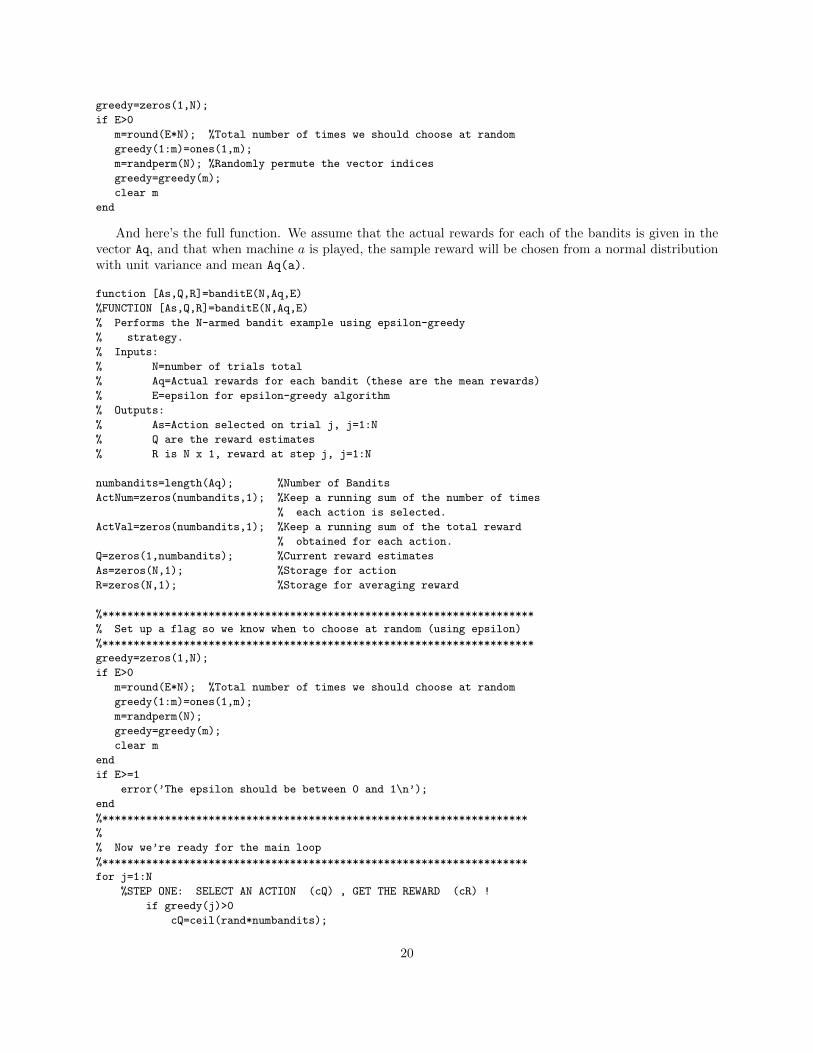
greedy=zeros(1,N);
if E>0
m=round(E*N); %Total number of times we should choose at random
greedy(1:m)=ones(1,m);
m=randperm(N); %Randomly permute the vector indices
greedy=greedy(m);
clear m
end
And here’s the full function. We assume that the actual rewards for each of the bandits is given in thevector Aq, and that when machine a is played, the sample reward will be chosen from a normal distributionwith unit variance and mean Aq(a).
function [As,Q,R]=banditE(N,Aq,E)
%FUNCTION [As,Q,R]=banditE(N,Aq,E)
% Performs the N-armed bandit example using epsilon-greedy
% strategy.
% Inputs:
% N=number of trials total
% Aq=Actual rewards for each bandit (these are the mean rewards)
% E=epsilon for epsilon-greedy algorithm
% Outputs:
% As=Action selected on trial j, j=1:N
% Q are the reward estimates
% R is N x 1, reward at step j, j=1:N
numbandits=length(Aq); %Number of Bandits
ActNum=zeros(numbandits,1); %Keep a running sum of the number of times
% each action is selected.
ActVal=zeros(numbandits,1); %Keep a running sum of the total reward
% obtained for each action.
Q=zeros(1,numbandits); %Current reward estimates
As=zeros(N,1); %Storage for action
R=zeros(N,1); %Storage for averaging reward
%*********************************************************************
% Set up a flag so we know when to choose at random (using epsilon)
%*********************************************************************
greedy=zeros(1,N);
if E>0
m=round(E*N); %Total number of times we should choose at random
greedy(1:m)=ones(1,m);
m=randperm(N);
greedy=greedy(m);
clear m
end
if E>=1
error(’The epsilon should be between 0 and 1\n’);
end
%********************************************************************
%
% Now we’re ready for the main loop
%********************************************************************
for j=1:N
%STEP ONE: SELECT AN ACTION (cQ) , GET THE REWARD (cR) !
if greedy(j)>0
cQ=ceil(rand*numbandits);
20
cR=randn+Aq(cQ);
else
[val,idx]=find(Q==max(Q));
m=ceil(rand*length(idx)); %Choose a max at random
cQ=idx(m);
cR=randn+Aq(cQ);
end
R(j)=cR;
%UPDATE FOR NEXT GO AROUND!
As(j)=cQ;
ActNum(cQ)=ActNum(cQ)+1;
ActVal(cQ)=ActVal(cQ)+cR;
Q(cQ)=ActVal(cQ)/ActNum(cQ);
end
Next we’ll create a test bed for the routine. We will call the program 2,000 times, and each call willconsist of 1,000 plays. We will set the number of bandits to 10, and change the value of � from 0 to 0.01 to0.1, and see what the average reward per play is over the 1000 plays.
Here’s a script file that we’ll use to call the banditE routine:
Ravg=zeros(1000,1);
E=0.1;
for j=1:2000
m=randn(10,1);
[As,Q,R]=banditE(1000,m,E);
Ravg=Ravg+R;
if mod(j,10)==0
fprintf(’On iterate %d\n’,j);
end
end
Ravg=Ravg./2000;
plot(Ravg);
The output of the algorithms are shown in Figure 2.1.
The Softmax Action Selection
In the Softmax action selection algorithm, the idea is to construct a set of probabilities. This set will havethe properties that:
• The machine (or arm) giving the highest estimated payoff will have the highest probability.
• We will choose a machine using the probabilities. For example, if the probabilities are 0.5, 0.3, 0.2 formachines 1, 2, 3 respectively, then machine 1 would be chosen 50% of the time, machine 2 would bechosen 30% of the time, and the last machine 20% of the time.
Therefore, this algorithm will maintain an exploration of all machines so that we will not get locked onto asuboptimal machine.
Now if we have n machines with estimated payoffs recorded as:
Q = [Qt(1), Qt(2), . . . , Qt(n)]
we want to construct n probabilities,
P = [Pt(1), Pt(2), . . . , Pt(n)]
The requirements for this transformation are:
21

Figure 2.1: Results of the testbed on the 10-armed bandit. Shown are the rewards given per play, averagedover 2000 trials.
1. Pt(k) ≥ 0 for k = 1, 2, . . . (because all probabilities are positive). Another way to say this is to saythat the range of the transformation is nonnegative.
2. If Qt(a) < Qt(b), then Pt(a) < Pt(b). That is, the transformation must be strictly increasing for alldomain values.
3. Finally, the sum of the probabilities must be 1.
A function that satisfies requirements 1 and 2 is the exponential function. It’s range is nonnegative. Itmaps large negative values (large negative payoffs) to near zero probability, and it is strictly increasing. Upto this point, the transformation is:
Pt(k) = eQt(k)
We need the probabilities to sum to 1, so we normalize the Pt(k):
Pt(k) =Pt(k)
Pt(1) + Pt(2) + . . .+ Pt(n)=
exp(Qt(k))�nj=1 exp(Qt(j))
This is a popular technique worth remembering- We have what is called a Gibbs (or Boltzmann) distribution.We could stop at this point, but it is convenient to introduce a control parameter τ (sometimes this is referredto as the temperature of the distribution). Our final version of the transformation is given as:
Pt(k) =exp
�Qt(k)
τ
�
�nj=1 exp
�Qt(j)
τ
�
EXERCISE: Suppose we have two probabilities, P (1) and P (2) (we left off the time index since it won’tmatter in this problem). Furthermore, suppose P (1) > P (2). Compute the limits of P (1) and P (2) as τ
22
goes to zero. Compute the limits as τ goes to infinity (Hint on this part: Use the definition, and dividenumerator and denominator by exp(Q(1)/τ) before taking the limit).
What we find from the previous exercise is that the effect of large τ (hot temperatures) makes all theprobabilities about the same (so we would choose a machine almost at random). The effect of small tau (coldtemperatures) makes the probability of choosing the best machine almost 1 (like the greedy algorithm).
In Matlab, these probabilities are easy to program. Let Q be a vector holding the current estimates ofthe returns, as before, and let t= τ , the temperature. Then we construct a vector of probabilities using thesoftmax algorithm:
P=exp(Q./t);
P=P./sum(P);
Programming Comments
1. How to select action a with probability p(a)?
We could do what we did before, and create a vector of choices with those probabilities fixed, but ourprobabilities change. We can also use the uniform distribution, so that if x=rand, and x ≤ p(1), useaction 1. If p(1) < x ≤ p(1) + p(2), choose action 2. If p(1) + p(2) < x ≤ p(1) + p(2) + p(3), chooseaction 3, and so on. There is an easy way to do this, but it is not optimal (in terms of speed). Weintroduce two new Matlab functions, cumsum and histc.
The function cumsum, which means cumulative sum, takes a vector x as input, and outputs a vector yso that y=cumsum(x) creates:
yk =
k�
n=1
xn = x1 + x2 + . . .+ xk
For example, if x = [1, 2, 3, 4, 5], then cumsum(x) would output [1, 3, 6, 10, 15]
The function histc (for histogram count) has the form: n=histc(x,y), where the vector y is mono-tonically increasing. The elements of y form “bins” so that n(k) counts the number of values in x thatfall between the elements y(k) (inclusive) and y(k+1) (exclusive) in the vector y. Try a particularexample, like:
Bins=[0,1,2];
x=[-2, 0.25, 0.75, 1, 1.3, 2];
N=histc(x, Bins);
Bins sets up the desired intervals as [0, 1) and [1, 2) and the last value is set up as its own interval, 2.Since −2 is outside of all the intervals, it is not counted. The next two elements of x are inside thefirst interval, and the next two elements are inside the second interval. Thus, the output of this codefragment is N = [2, 2, 1].
Now in our particular case, we set up the bin edges (intervals) so that they are the cumulative sums.We’ll then choose a number between 0 and 1 using the (uniformly) random number x = rand, anddetermine what interval it is in. This will be our action choice:
P=[0.3, 0.1, 0.2, 0.4];
BinEdges=[0, cumsum(P)];
x=rand;
Counts=histc(x,BinEdges);
ActionChoice=find(Counts==1);
23
2. We have to change our parameter τ from some initial value τinit (big, so that machines are chosenalmost at random) to some small final value, τfin. There are an infinite number of ways of doing this.For example, a linear change from a value a to a value b in N steps would be the equation of the linegoing from the point (1, a) to the point (N, b).
Exercise: Give a formula for the parameter update, τ in terms of the initial value, τinit and the finalvalue, τfin if we use a linear decrease as t ranges from 1 to N .
A more popular technique is to use the following formula, which we’ll use to update many parameters.Let the initial value of the parameter be given as a, and the final value be given as b. Then theparameter p is computed as:
p = a ·�b
a
�t/N
(2.2)
Note that when t = 0, p = a and when t = N , p = b1
“Win-Stay, Lose-Shift” Strategy
The “Win-Stay, Lose-Shift” strategy discussed in terms of Harlow’s monkeys and perhaps the probabilitymatching experiments of Estes might be re-formulated here for the n−armed bandit experiment.
In this experiment, we interpret the strategy as: If I’m winning, make the probability of choosing thataction stronger. If I’m losing, make the probability of choosing that action weaker. This brings us to theclass of pursuit methods.
Define a∗ to be the winning machine at the moment, i.e.,
a∗ = maxa
Qt(a)
The idea now is straightforward- Slightly increase the probability of choosing this winning machine, andcorrespondingly decrease the probability of choosing the others.
Define the probability of choosing machine a as P (a) (or, if you want to explicitly include the time index,Pt(a). Then given the winning machine index as a∗, we update the current probabilities by using a parameterβ ∈ [0, 1]:
Pt+1(a∗) = Pt(a
∗) + β [1− Pt(a∗)]
and the rest of the probabilities decrease towards zero:
Pt+1(a) = Pt(a) + β [0− Pt(a)]
Exercises with the Pursuit Strategy
1. Suppose we have three probabilities, P1, P2, P3, and P1 is the unique maximum. Show that, for anyβ > 0, the updated values still sum to 1.
2. Using the same values as before, show that, for any β > 0, the updated values will stay between 0 and1- that is, If 0 ≤ Pi ≤ 1 for all i before the update, then after the update, 0 ≤ Pi ≤ 1.
3. Here is one way to deal with a tie (show that the updated values still sum to 1): If there are k machineswith a maximum, update each via:
Pt+1 = (1− β) ∗ Pt + β/k
4. Suppose that for some fixed j, Pj is always a loser (never a max). Show that the update rule guaranteesthat Pj → 0 as t → ∞. HINT: Show that Pj(t) = (1− β)tPj(0)
5. Suppose that for some fixed j, Pj is always a winner (with no ties). Show that the update ruleguarantees that Pj → 1 as t → ∞.
1In the C/C++ programming language, indices always start with zero, and this is leftover in this update rule. This is nota big issue, and the reader can make the appropriate change to starting with t = 1 if desired.
24
Matlab Functions softmax and winstay
Here are functions that will yield the softmax and win-stay, lose-shift strategies. Below each is a driver.Read through them carefully so that you understand what each does. We’ll then ask you to put these intoMatlab and comment on what you see.
function a=softmax(EstQ,tau)
% FUNCTION a=softmax(EstQ, tau)
% Input: Estimated payoff values in EstQ (size 1 x N,
% where N is the number of machines
% tau - "temperature": High values- the probs are all
% close to equal; Low values, becomes "greedy"
% Output: The machine that we should play (a number between 1 and N)
if tau==0
fprintf(’Error in the SoftMax program-\n’);
fprintf(’Tau must be greater than zero\n’);
a=0;
return
end
Temp=exp(EstQ./tau);
S1=sum(Temp);
Probs=Temp./S1; %These are the probabilities we’ll use
%Select a machine using the probabilities we just computed.
x=rand;
TotalBins=histc(x,[0,cumsum(Probs)’]);
a=find(TotalBins==1);
Here is a driver for the softmax algorithm. Note the implementation details (e.g., how the “actual”payoffs are calculated, and what the initial and final parameter values are):
%Script file to run the N-armed bandit using the softmax strategy
%Initializations are Here:
NumMachines=10;
ActQ=randn(NumMachines,1); %10 machines
NumPlay=1000; %Play 100 times
Initialtau=10; %Initial tau ("High in beginning")
Endingtau=0.5;
tau=10;
NumPlayed=zeros(NumMachines,1); %Keep a running sum of the number
% of times each action is selected
ValPlayed=zeros(NumMachines,1); %Keep a running sum of the total
% reward for each action
EstQ=zeros(NumMachines,1);
PayoffHistory=zeros(NumPlay,1); %Keep a record of our payoffs
for i=1:NumPlay
%Pick a machine to play:
a=softmax(EstQ,tau);
25

%Play the machine and update EstQ, tau
Payoff=randn+ActQ(a);
NumPlayed(a)=NumPlayed(a)+1;
ValPlayed(a)=ValPlayed(a)+Payoff;
EstQ(a)=ValPlayed(a)/NumPlayed(a);
PayoffHistory(i)=Payoff;
tau=Initialtau*(Endingtau/Initialtau)^(i/NumPlay);
end
[v,winningmachine]=max(ActQ);
winningmachine
NumPlayed
plot(1:10,ActQ,’k’,1:10,EstQ,’r’)
Here is the function implementing the pursuit strategy (or “Win-Stay, Lose-Shift”).
function [a, P]=winstay(EstQ,P,beta)
% function [a,P]=winstay(EstQ,P,beta)
% Input: EstQ, Estimated values of the payoffs
% P = Probabilities of playing each machine
% beta= parameter to adjust the probabilities, between 0 and 1
% Output: a = Which machine to play
% P = Probabilities for each machine
[vals,idx]=max(EstQ);
winner=idx(1); %Index of our "winning" machine
%Update the probabilities. We need to do P(winner) separately.
NumMachines=length(P);
P(winner)=P(winner)+beta*(1-P(winner));
Temp=1:NumMachines;
Temp(winner)=[]; %Temp now holds the indices of all "losers"
P(Temp)=(1-beta)*P(Temp);
%Probabilities are all updated- Choose machine a w/prob P(a)
x=rand;
TotalBins=histc(x,[0,cumsum(P)’]);
a=find(TotalBins==1);
And its corresponding driver is below. Again, be sure to read and understand what each line of the codedoes:
%Script file to run the N-armed bandit using pursuit strategy
%Initializations
NumMachines=10;
ActQ=randn(NumMachines,1);
NumPlay=2000;
Initialbeta=0.01;
Endingbeta=0.001;
beta=Initialbeta;
NumPlayed=zeros(NumMachines,1);
26
ValPlayed=zeros(NumMachines,1);
EstQ=zeros(NumMachines,1);
Probs=(1/NumMachines)*ones(10,1);
for i=1:NumPlay
%Pick a machine to play:
[a,Probs]=winstay(EstQ,Probs,beta);
%Play the machine and update EstQ, tau
Payoff=randn+ActQ(a);
NumPlayed(a)=NumPlayed(a)+1;
ValPlayed(a)=ValPlayed(a)+Payoff;
EstQ(a)=ValPlayed(a)/NumPlayed(a);
beta=Initialbeta*(Endingbeta/Initialbeta)^(i/NumPlay);
end
[v,winningmachine]=max(ActQ);
winningmachine
NumPlayed
plot(1:10,ActQ,’k’,1:10,EstQ,’r’)
Homework: Implement these 4 pieces of code into Matlab, and comment on the performance of each.You might try changing the initial and final values of the parameters to see if the algorithms are stable tothese changes. As you form your comments, recall our two competing goals for these algorithms:
• Estimate the values of the actual payoffs (more accurately, the mean payout for each machine).
• Maximize our rewards!
2.2.3 A Summary of Reinforcement Learning
We looked in depth at a basic problem of unsupervised learning- That of trying to find the best winning slotmachine in a bank of many. This problem was unsupervised because, although we got rewards or punishmentsby winning or losing money, we did not know at the beginning of the problem what those payoffs would be.That is, there was no expert available to tell us if we were doing something correctly or not, we had to infercorrect behavior from directly playing the machines.
We also saw that to solve this problem, we had to do a lot of trial and error learning- that’s typical inunsupervised learning. Because an expert is not there to tell us the operating parameters, we have to spendtime exploring the possibilities.
We learned some techniques for translating learning theory into mathematics, and in the process, welearned some commands in Matlab. We don’t expect you to be an expert programmer - this should be afairly gentle introduction to programming. At this stage, you should be able to read some Matlab code andinterpret the output of an algorithm. Later on, we’ll give you more opportunities to produce your own piecesof code.
In summary, we looked at the greedy algorithm, the �−greedy algorithm, the softmax strategy, and thepursuit strategy. You might consider how closely (if at all) these algorithms would reproduce human oranimal behavior if given the same task.
There are many more topics in Reinforcement Learning to consider, we presented only a short introductionto the topic.
27

28

Chapter 3
Statistics
As we have discussed previously, statistics will naturally emerge when we have to deal either with modelsthat have random characteristics, or with data that may incorporate some kind of random noise. Generallyspeaking, models will typically involve a deterministic component and a random component.
In this section, we’ll briefly give an overview of some common statistical vocabulary and computations.
3.1 Functions that Define Data
The basic way of defining non-deterministic data is through the use of a probability density function, or pdf.
Example 1: Given a fair dice, the probablity of rolling any number from 1 to 6 is equally likely. If welet f(x) be the probability that we get x, then in this case:
f(1) = f(2) = f(3) = f(4) = f(5) = f(6) =1
6
In this case, f is our pdf.
Example 2: Given the 14 points:
{1, 2, 3, 2, 1, 1, 2, 3, 3, 2, 2, 1, 1, 1}
we might deduce that the probability of having “1” is 6/14, the probability of getting a “2” is 5/14, and theprobability of getting a 3 is 3/14. Thus the pdf is:
f(1) =6
14f(2) =
5
14f(3) =
3
14
In this case, we would assume that the process generating these numbers is adequately represented by thisset- For example, the process is only generating the numbers 1, 2 and 3, and we have sampled long enough toget a good approximation to the frequency of each number. This is what is called a “frequentist” approachto building a probability density function.
Definition: A (continuous) function f(x) is said to be a probability density function if it satisfies thefollowing conditions:
1. f(x) is always non-negative.
2.�∞−∞ f(x) dx = 1
29
3. The probability of an event between values x = a and x = b is given by:
Pr(a ≤ X ≤ b) =
� b
a
f(x) dx
Definition: A discrete probability density function will be a finite set of numbers, {P1, P2, . . . , Pk}, so that:
1. Pi is non-negative, for all i.
2.
k�
i=1
Pk = 1
Let’s take a look at some template probability distributions:
• The Uniform Distribution
– The Continuous Version:
f(x) =
�1
b−a , if a ≤ x ≤ b
0, otherwise
– The Discrete Version (using N bins over the same interval):
Pr
�a+ (i− 1)
b− a
N≤ x ≤ a+ i
b− a
N
�=
1
N= Pi, i = 1, 2, . . . , N.
– In Matlab, to obtain a value from a uniform distribution over [0, 1], we type x = rand
• The Normal (or Gaussian) Distribution
– The Continuous Version: The Normal distribution with mean µ and variance σ2 (to be definedshortly) is defined as:
f(x) =1√2π σ
exp
�−(x− µ)2
σ2
�
This is the common “bell-shaped curve”; the constant in the front is needed to make the integralevaluate to 1. Note that the normal distribution with zero mean and variance 1 simplifies to:
f(x) = N (0, 1) =1√2π
e−x2
– In Matlab, we can obtain values from a normal distribution with zero mean and unit variance byx = randn.
• The Double Laplacian.
Our last example we define only in the continuous case. It is the p.d.f. commonly used to model thehuman voice, and is called the double Laplacian distribution:
f(x) =
�Ke−|x|, −1 ≤ x ≤ 10, otherwise
In the exercises, you’ll be asked to determine the value of K, and we’ll also see how the shape of theLaplacian compares to a normal distribution.
30

3.1.1 The probability distribution function
The probability distribution function (a.k.a. distribution function, cumulative distribution function) is de-fined via the probability density function:
F (X) = Pr(−∞ < X < x) =
� x
−∞f(t) dt
We note that:
• By the Fundamental Theorem of Calculus, part I, F (x) is the antiderivative of f(x).
• F (x) is strictly increasing, going from a minimum of zero to a maximum of 1.
• To minimize confusion between terms, we’ll refer to F (x) as the distribution function, or cumulativedistribution function. We’ll also reserve capitalized letters for the distribution function, and small-caseletters for the probability density function.
3.2 The Mean, Median, and Mode
The most basic way to characterize a data set is through one number- the mean (or median or mode).
• The Sample Mean for a discrete set of m numbers, x1, . . . , xm is given by:
x =1
m
m�
k=1
xk
We will typically use the sample mean rather than the population mean, which is defined using theunderlying pdf:
µ = E(X) =�
all x
xf(x)
You might remember this formula by seeing that this is really a weighted average, with those eventsmost probable getting a higher weight than events less probable.
Also, if your data is being drawn independently from a fixed p.d.f., then the sample mean will convergeto the population mean, as the number of samples gets very large.
Suppose we have m vectors in IRn. we can similarly define the (sample) mean, just replace the scalarxk with the kth vector:
x =1
m
m�
k=1
x(k)
The jth element of the sample mean vector is just the sample mean of the (scalar) data in the jth
dimension of your collection of vectors.
In Matlab, the mean is a built-in function. The command is mean, and the output depends on whetheryou input a vector or a matrix of data.
For vectors, mean(x) outputs a scalar.
m=mean(X,1); %Returns a row vector
m=mean(X,2); %Returns a column vector
For matrices, one can compute a row mean (which is a row), a column mean (which is a column) ora grand mean. In this context, the grand mean of a matrix is found by taking the mean of all theentries of the matrix, so the grand mean of a matrix is a scalar.
See the end of this section for more on mean subtracting a matrix of data.
31

• The Median is a number so that exactly half the data is above that number, and half the data is belowthat number. Although the median does not have to be unique, we follow the definitions below if weare given a finite sample:
If there are an odd number of data points, the median is the middle point. If there is an even numberof data points, then there are two numbers in the middle- the median is the average of these.
Although not used terribly often, Matlab will perform the median as well as the mean:
m=median(X);
where the output is a scalar if X is a vector, or a row vector if X is a matrix.
• The Mode is the value taken the most number of times. In the case of ties, the data is multi-modal.
We’ll compare these definitions in the Exercises.
3.2.1 Centering and Double Centering Data
Let matrix A be n×m, which may be considered n points in Rm or m points in IRn. If we wish to look atA both ways, a double-centering may be appropriate.
The result of the double-centering will be that (in Matlab), we determine A so that
mean(A, 1) = 0, mean(A, 2) = 0
The algorithm is (in Matlab):
%Let A be n times m
[n,m]=size(A);
rowmean=mean(A);
A1=A-repmat(rowm,n,1);
colmean=mean(A1,2);
Ahat=A1-repmat(colmean,1,m);
or, equivalently:
%Let A be n times m
[n,m]=size(A);
colmean=mean(A,2);
A1=A-repmat(colmean,1,m);
rowmean=mean(A1,1);
Ahat=A1-repmat(rowmean,n,1);
Proof: For the first version (row mean first):Let A1 be the matrix A with the row mean b subtracted:
A1 =
a11 − b1 a12 − b2 · · · a1m − bma21 − b1 a22 − b2 · · · a2m − bm
......
an1 − b1 an2 − b2 · · · anm − bm
with
bj =1
n
n�
i=1
aij
32

Now define c as the column mean of A1. Mean subtraction of this column results in the A, writtenexplicitly as:
A =
a11 − b1 − c1 a12 − b2 − c1 · · · a1m − bm − c1a21 − b1 − c2 a22 − b2 − c2 · · · a2m − bm − c2
......
an1 − b1 − cn an2 − b2 − cn · · · anm − bm − cn
By definition, the column mean of A is zero. Is the new row mean zero? It is clear that the new row meanis zero iff
�k ck = 0, which we now show:
Proof that
n�
k=1
ck = 0
We explicitly write down what ck is:
ck =1
m
m�
j=1
(akj − bj)
and substitute the expression for bj ,
ck =1
m
m�
j=1
�akj −
1
n
n�
i=1
aij
�=
1
m
m�
j=1
akj −1
mn
m�
j=1
n�
i=1
aij
Now sum over k:n�
k=1
ck =
n�
k=1
1
m
m�
j=1
akj −1
mn
m�
j=1
n�
i=1
aij
=
1
m
n�
k=1
m�
j=1
akj −n
mn
m�
j=1
n�
i=1
aij = 0
It may be clear that these two methods produce the same result (e.g., row subtract first, then columnsubtract or vice-versa). If we examine the (i, j)th entry of A,
Aij = aij − bj − ci = aij −1
n
n�
k=1
akj −1
m
m�
k=1
aik +
m�
r=1
n�
s=1
ars
Therefore, to double center a matrix of data, each element has subtracted from it its corresponding rowmean and column mean, and we add back the average of all the elements.
As a final note, this technique is only suitable if it is reasonable that the m × n matrix may be data ineither IRn or IRm. For example, you probably would not double center a data matrix that is 5000× 2 unlessthere is a specific reason to do so.
Example
Let the matrix be defined below. Verify that the row mean, column mean are vectors with all 1’s and thegrand mean is 1 as well. After that, double center the array.
�3 0 −1 2
−1 2 3 0
�
SOLUTION: Computing the means, we see that the row mean is [1111] the column mean is [1, 1]T and thegrand mean is also 1! Double centering means we’ll subtract the row and column mean, then add back inthe grand mean. In this special matrix, that means that we’ll subtract 1 from every value:
�3 0 −1 2
−1 2 3 0
�→
�2 −1 −2 1
−2 1 2 −1
�
Now you should notice that the new row mean and new column mean are vectors with all zeros.
33

3.3 The Variance and Standard Deviation
The number that is used to describe the spread of the data about its mean is the variance. As with themean, we rarely know the underlying distribution, so again we’ll focus on the sample variance.
Let {x1, . . . , xm} be m real numbers. Then the sample variance is:
s2 =1
m− 1
m�
k=1
(xk − x)2
where x is the mean of the data. If we think of the data as a vector of length m, then this formula becomes:
s2 =1
m− 1�x− x�2
To be complete, we include the population variance below:
σ2 = E((x− µ)2) =�
all x
(x− µ)2f(x)
Finally, the standard deviation is the square root of the variance, so the standard deviation is σ.
Quick Example
Let’s take some template data to look at what the variance (and standard deviation) measure: Consider thedata:
− 2
n,− 1
n, 0,
1
n,2
n
If n is large, our data is tightly packed together about the mean, 0. If n is small, the data are spread out.The variance of this sample is:
s2 =1
4
�4 + 1 + 0 + 1 + 4
n2
�=
5
2
1
n2
so that the standard deviation is:
s =
�5
2
1
n
and this is in agreement with our heuristic: If n is large, our data is tightly packed about the mean, and thestandard deviation is small. If n is small, our data is loosely distributed about the mean, and the standarddeviation is large. Another way to look at the standard deviation is in linear algebra terms: If the data isput into a vector of length m (call it x), then the (sample) standard deviation can be computed as:
s =�x�√m− 1
3.3.1 Covariance and Correlation Coefficients
If we have two data sets, sometimes we would like to compare them to see how they relate to each other. Inthis case, it is important that the two data sets be ordered so that x1 is being compared to y1, then x2 iscompared to y2, and so on.
Definition: Let X = {x1, . . . , xn} , Y = {y1, . . . , yn} be two ordered data sets with means mx,my
respectively. Then the sample covariance of the data sets is given by:
Cov(X,Y ) = s2xy =1
n− 1
n�
k=1
(xk −mx)(yk −my)
34

There are exercises at the end of the chapter that will reinforce the notation and give you some methodsfor manipulating the covariance. In the meantime, it is easy to remember this formula if you think of thefollowing:
If X and Y have mean zero, and we think of X and Y as vectors x and y, then the covariance is just thedot product between the vectors, divided by n− 1:
Cov(x,y) =1
n− 1xTy
We can then interpret what it means for X,Y to have a covariance of zero: x is “orthogonal” to y.Continuing with this analogy, if we normalized by the size of x and the size of y, we’d get the cosine of theangle between them. This is the definition of the correlation coefficient, and gives the relationship betweenthe covariance and correlation coefficient:
Definition: The correlation coefficient between x and y is given by:
rxy =s2xysxsy
=
�nk=1(xk −mx)(yk −my)��n
k=1(xk −mx)2 ·�n
k=1(yk −my)2
Again, thinking of X,Y as having zero mean and placing the data in vectors x,y, then this formula becomes:
rxy =xTy
�x� · �y� = cos(θ)
This works out so nicely because we have a 1n−1 in both the numerator and denominator, so they cancel
each other out.We also see immediately that rxy can only take on the real numbers between −1 and 1. Some interesting
values of rxy:
If rxy is: Then the data is:1 Perfectly correlated (θ = 0)0 Uncorrelated (θ = π
2 )-1 Perfectly (negatively) correlated (θ = π)
One last comment before we leave this section: The covariance s2xy and correlation coefficient rxy onlylook for linear relationships between data sets!
For example, we know that sin(x) and cos(x) (as functions, or as data points sampled at equally spacedintervals) will be uncorrelated, but, because sin2(x) + cos2(x) = 1, we see that sin2(x) and cos2(x) areperfectly correlated.
This difference is the difference between the words “correlated” and “statistically independent”. Statisti-cal independence (not defined here) and correlations are not the same thing! We will look at this differenceclosely in a later section.
3.4 The Covariance Matrix
If we have p data points in IRn, we can think of the data as a p×n matrix. Let X denote the mean-subtracteddata matrix (as we defined previously). A natural question to ask is then how the ith and jth dimensions(columns) covary- so we’ll compute the covariance between the i, j columns to define:
s2ij =1
p− 1
p�
k=1
X(k, i) ·X(k, j)
Computing this for all i, j will result in an n× n symmetric matrix, C, for which:
Cij = s2ij
35
In the exercises, you’ll show that an alternative way of computing the covariance matrix is by using whatwe’ll refer to as its definition:
Definition: Let X denote a matrix of data, so that, if X is p × n, then we have p data points in IRn.Furthermore, we assume that the data in X has been mean subtracted (so the mean in IRn is the zerovector). Then the covariance matrix associated with X is given by:
C =1
p− 1XTX
In Matlab, it is easy to compute the covariance matrix. For your convenience, we repeat the mean-subtraction routine here:
%X is a pxn matrix of data:
[p,n]=size(X);
m = mean(X);
Xm = X-repmat(m,p,1);
C=(1/(p-1))*X’*X;
Matlab also has a built-in covariance function. It will automatically do the mean-subtraction (which isa lot of extra work if you’ve already done it!).
C=cov(X);
If you forget which sizes Matlab uses, you might want to just compute the covariance yourself. It assumes,as we did, that the matrix is p×n, and returns an n×n covariance, and it will divide by p−1 (some algorithmdivide only by p).
3.5 Exercises
1. By hand, compute the mean and variance of the following set of data:
1, 2, 9, 6, 3, 4, 3, 8, 4, 2
2. Obtain a sampling of 1000 points using the uniform distribution: and 1000 points using the normaldistribution:
x=rand(1000,1);
y=randn(1000,1);
Compare the distributions using Matlab’s hist command: hist([x y],100) and print the results.You’ll note that the histograms have not been scaled so that the areas sum to 1, but we do get anindication of the nature of the data.
3. Compute the value of K in the double Laplacian function so that f is a p.d.f.
4. Next, load a sample of human voice: load laughter If you type whos, you’ll see that you have a vectory with the sound data. The computers in the lab do have sound cards, but they don’t work very wellwith Matlab, so we won’t listen to the sample. Before continuing, you might be curious about whatthe data in y looks like, so feel free to plot it. We want to look at the distribution of the data in thevector y, and compare it to the normal distribution. The mean of y is already approximately zero, butto get a good comparison, we’ll take a normal distribution with the same variance:
36

clear
load laughter
whos
sound(y,Fs); %This only works if there’s a good sound card
s=std(y);
x=s*randn(size(y));
hist([x y],100); %Blue is "normal", Red is Voice
Print the result. Note that the normal distribution is much flatter than the distribution of the voicesignal.
5. Compute the covariance between the following data sets:
x −1.0 −0.7 −0.4 −0.1 0.2 0.5 0.8y −1.3 −0.7 −0.1 0.5 1.1 1.7 2.3
(3.1)
6. Let x be a vector of data with mean µ, and let a, b be scalars. What is the mean of ax? What is themean of x+ b? What is the mean of ax+ b?
NOTE: Formally, the addition of a vector and a scalar is not defined. Here, we are utilizing Matlabnotation: The result of a vector plus a scalar is addition done component-wise. This is only done withscalars- for example, a matrix added to a vector is still not defined, while it is valid to add a matrixand a scalar.
7. Let x be a vector of data with variance σ2, and let a, b be scalars. What is the variance of ax? Whatis the variance of x+ b? What is the variance of ax+ b?
8. Show that, for data in vectors x, y and a real scalar a,
Cov(ax, y) = aCov(x, y) Cov(x, by) = bCov(x, y)
9. Show that, for data in x and a vector consisting only of the scalar a,
Cov(x, a) = 0
10. Show that, for a and b fixed scalars, and data in vectors x,y,
Cov(x+ a, y + b) = Cov(x, y)
11. If the data sets X and Y are the same, what is the covariance? What is the correlation coefficient?What if Y = mX? What if Y = mX + b?
12. Let X be a p× n matrix of data, where we n columns of p data points (you may assume each column
has zero mean). Show that the (i, j)th entry of1
p− 1XTX is the covariance between the ith and jth
columns of X. HINT: It might be convenient to write X in terms of its columns,
X = [x1,x2, . . . ,xn]
Also show that 1p−1X
TX is a symmetric matrix.
13. This exercise shows us that our geometric insight might not extend to high dimensional space. Weexamine how points are distributed in high dimensional hypercubes and unit balls. Before we begin,let us agree that a hypercube of dimension n has the edges:
(±1,±1,±1, . . . ,±1)T
so, for example, a 2-d hypercube (a square) has edges:
(1, 1)T , (−1, 1)T , (1,−1)T , (−1,−1)T
37

(a) Show that the distance (standard Euclidean) from the origin to a corner of a hypercube of dimen-sion d is
√d. What does this imply about the shape of the “cube”, as d → ∞?
(b) The volume of a d−dimensional hypersphere of radius a can be written as:
Vd =Sda
d
d
where Sd is the d−dimensional surface area of the unit sphere.
First, compute the volume between hyperspheres of radius a and radius a− �.
Next, show that the ratio of this volume to the full volume is given by:
1−�1− �
a
�d
What happens as d → ∞?
If we have 100,000 data points “uniformly distributed” in a hypersphere of dimension 10,000,where are “most” of the points?
3.6 Linear Regression
In this section, we examine the simplest case of fitting data to a function. We are given p pairs of data (t isfor “target”, we’ll use y for something else):
(x1, t1), (x2, t2), . . . (xp, tp)
We wish to find a line through the data. That is, we want to find scalars m, b so that
mxi + b = ti
for each pair (xi, ti). Of course, if the data actually was on a line, we would not need p points- only two areneeded.
Thus, we assume that there is something going on so that the data is not exactly linear (statisticianswould add �i to the end of our line to account for noise). Thus, for each point, we now have an error. Weare distinguishing now between the point on the line:
yi = mxi + b
and the desired value ti. Now the error at the ith point is defined as:
(ti − yi)2 = (ti − (mxi + b))2
and the overall error is the sum of squares error (summed over the p points):
E(m, b) =
p�
k=1
(tk − (mxk + b))2
We have now translated our problem into a Calculus problem- Find the minimum of E(m, b). Here are someexercises to lead you to the solution:
Exercises with the Regression Error
1. E is a function of m and b, so the minimum value occurs where
∂E
∂m= 0
∂E
∂b= 0
38

Show that this leads to the system of equations: (the summation index is 1 to p)
m�
x2k + b
�xk =
�xktk
m�
xk + bn =�
tk
2. Using linear algebra, given the data, then in finding the line of best fit, we are trying to solve thesystem of equations below, where we then write the system in matrix-vector form:
mx1 + b = t1mx2 + b = t2mx3 + b = t3
......
mxp + b = tp
⇒
x1 1x2 1x3 1...
...xp 1
�mb
�=
t1t2...
tp
⇒ Ac = t
As we said before, the data does not lie exactly on a line (otherwise we would only need two points).That means that this system of equations has no solution. However, if we think of varying the vectorof unknowns c, we might define the model output as y:
y = Ac
Now we can define the error as:
E(c) = �t− y�2 = �t−Ac�2
and now we will find c that minimizes this error- In linear algebra, this is known as the least squaressolution to the equation Ac = t. We will revisit this again later using projections, but for now, we cansolve this problem using the normal equations. That is, we will multiply both sides of our equationby AT to get:
Ac = t ⇒ ATAc = AT t
Originally, A was p×2, so now ATA is 2×2, which we can invert. EXERCISE: Show that this system oftwo equations in two variables is the same as the system we obtained by setting the partial derivativesto zero.
3. Consider the following data set [11] which relates the index of exposure to radioactive contaminationfrom Hanford to the number of cancer deaths per 100, 000 residents. We would like to get a relationshipbetween these data.
County/City Index Deaths
Umatilla 2.5 147Morrow 2.6 130Gilliam 3.4 130Sherman 1.3 114Wasco 1.6 138Hood River 3.8 162Portland 11.6 208Columbia 6.4 178Clatsop 8.3 210
39

40