An Introduction to Mechanism Design

Theory ∗

Debasis Mishra†

May 29, 2008

Abstract

The Nobel prize in economics was awarded to Leonid Hurwicz, Roger B. Myerson,

and Eric S. Maskin in 2007 for “having laid the foundations of mechanism design

theory”. This article aims to explore these very foundations of mechanism design

theory. In the process, it highlights one important contribution each of Myerson and

Maskin, and describes some fundamental concepts of mechanism design, which are due

to Hurwicz. While it briefly describes Maskin’s Nash implementation work, it goes

into the details of Myerson’s optimal auction design work, its extensions, and ongoing

work.

∗I thank Abhiroop Mukhopadhyay and Arunava Sen for their comments on an earlier version of this

article. Special thanks to V. R. Panchamukhi for his invitation to write this survey.†Indian Statistical Institute, 7 S.J.S. Sansanwal Marg, New Delhi - 110016, India

1

1 Introduction

Consider a seller who owns an indivisible object, say a house, and wants to sell to a set of

buyers. Each buyer has a value for the object, which is the utility of the house to the buyer.

The seller wants to design a selling procedure, an auction for example, such that he gets

the maximum possible price (revenue) by selling the house. If the seller knew the values of

the buyers, then he would simply offer the house to the buyer with the highest value and

give him a “take-it-or-leave-it” offer at a price equal to that value. Clearly, the (highest

value) buyer has no incentive to reject such an offer. Now, consider a situation where the

seller is unaware of the values of the buyers. What selling procedure will give the seller the

maximum possible revenue? A clear answer is impossible if the seller knows nothing about

the values of the buyer. However, the seller may have some information about the values of

the buyers. For example, the possible range of values, the probability of having these values

etc. Given these information, is it possible to design a selling procedure that guarantees

maximum (expected) revenue to the seller?

In this example, the seller had a particular objective in mind - maximizing revenue. Given

his objective he wanted to design a selling procedure such that when buyers participate in

the selling procedure and try to maximize their own payoffs within the rules of the selling

procedure, the seller will maximize his expected revenue over all such selling procedures.

The study of mechanism design looks at such issues. A planner needs to design a mech-

anism (a selling procedure in the above example) where strategic agents can interact. The

interactions of agents result in an outcome. While there are several possible ways to do de-

sign the rules, the planner has a particular objective in mind. For example, the objective can

be efficiency (maximization of the total welfare of agents) or maximization of his own surplus

(as was the case in the last example). Depending on the objective, the mechanism needs

to be designed in a manner such that when strategic agents interact, the resulting outcome

gives the desired objective. One can think of mechanism design as the reverse engineering of

game theory. In game theory terminology, a mechanism induces a game whose equilibrium

outcome is the objective that the mechanism designer has set.

The Nobel prize in economics was awarded to Leonid Hurwicz, Roger B. Myerson, and

Eric S. Maskin in 2007 for “having laid the foundations of mechanism design theory”. This

article aims to explore these very foundations of mechanism design theory. Since the liter-

ature is too large to cover in a brief survey, I focus on important contributions of the three

laureates. While I will be brief on the contributions of Huwicz and Maskin, I will be more

elaborate on the work of Myerson, mainly because it is an active research area currently.

Before I begin a formal treatment of mechanism design, let me motivate it by giving some

recent success stories of this theory in practice.

2

1.1 Some Applications

If a theory is judged by the applications it has in practice, then the mechanism design theory

passes this test. A recent book (Cramton et al., 2006) on combinatorial auctions, where a

set of objects are sold to a set of buyers who have value on bundles of goods, goes into

the details of many such applications. Below, I will describe two recent success stories of

mechanism design in practice.

The Spectrum Auction Design

The spectrum licences in US is auctioned by Federal Communications Commission (FCC)

almost every year. It raises enormous revenues - from 1994 to 2001, the revenue from these

auctions is about 40 billion US dollars. The sale of spectrum is a classic case of (multi-object

or combinatorial) auction design. Usually spectrum licences are auctioned separately for

various regions. However, spectrum licences for adjoining regions show synergy, i.e., if one

obtains licences for two neighboring states his value of the two licences will be higher than

sum of values of these licences. Auctioning licences separately cannot capture such synergies

of bidders. Such issues led to rethinking of the auction design by FCC. Prominent economic

theorists suggested their proposals to the FCC on how best to design auctions for selling

spectrum licences (Cramton, 2002). This led to major redesign of spectrum auctions by the

FCC, and subsequent increase in revenues.

Other countries in the world, including India and many countries in Europe, have used

auctions to sell spectrum licences. Because of the amount of revenue it generates, the appli-

cation of auctions in these settings remain one of the biggest success stories of mechanism

design.

The Sponsored Search Auction Design

Prominent Internet search companies use auctions as a means of generating revenue. When

we enter a keyword, say “Running Shoes”, for searching in Google, we see a list of advertise-

ments on the right hand side of the screen once the search is visible. Google auctions the slots

on these search pages dynamically to companies, e.g., in case of “Running Shoes” companies

like Nike and Reebok may be bidders for slots. Such auctions are popularly called sponsored

search auctions (SSA). While the technology behind conducting SSA in fractions of a sec-

ond is elegant, the design of such SSA have generated enormous interests (Edelman et al.,

2007). Google claims to use a“generalized” second-price auction, which we will describe later

(Edelman et al. (2007) show that this is not the appropriate generalization). To understand

the stakes involved in SSA, I note that Google’s revenues in 2005 was about 6 billion US dol-

lars, 90 percent of which came from revenues of such auctions. A recent book (Nisan et al.,

3

2007) goes into the theory of sponsored search auction design.

The rest of the essay is organized as follows. In Section 2, I give a general model of

mechanism design and describe some fundamental results. Since Hurwicz laid the foundations

of mechanism design, several concepts I describe in Section 2 reflect the contributions of

Hurwicz. I go into some details of Hurwicz’s contributions in Section 3. In Section 4, I

describe the optimal auction design work in Myerson (1981). In Section 5, I describe the

Nash implementation work in Maskin (1999). I conclude in Section 6.

2 A General Framework of Mechanism Design

2.1 A General Model

The set of agents is denoted by N = 1, . . . , n. The set of potential social decisions (or

outcomes) is denoted by the set D, which can be finite or infinite. Every agent has a

private information, called his type. The type of agent i ∈ N is denoted by θi which lies

in some set Θi. I emphasise that θi can be multi-dimensional. I denote a profile of types as

θ = (θ1, . . . , θn) and the cross product of type spaces of all agents as Θ = ×i∈NΘi.

Agents have preferences over decisions which depends on their respective types. This is

captured using a utility function. The utility function of agent i ∈ N is vi : Θi × D → R.

Thus, vi(d, θi) denotes the utility of agent i ∈ N for decision d ∈ D when his type is θi ∈ Θi.

I will restrict attention to this setting, called the private values setting, where the utility

function of an agent is independent of the types of other agents. Below are two examples to

illustrate the ideas.

A Public Project

Suppose a bridge needs to be built across a river in a city. The residents need to take a

decision whether to build the bridge or not. Hence, D = 0, 1, where 0 indicates that the

bridge is not built and 1 indicates that it is built. There is a total cost c from building the

bridge which the residents share. The value for the bridge for resident i ∈ N is θi ∈ R (his

type). Hence, utility of agent i with type θi when the decision is d ∈ 0, 1 can be written

as vi(d, θi) = d(

θi −cn

)

. This utility function has a particular form. The utility is linear in

the payment ( cn) of the agent. Such utility functions are called quasi-linear utility functions.

Allocating Multiple Objects

A set of indivisible goods M = 1, . . . , m need to be allocated to a set of agents N =

1, . . . , n. Let Ω = S : S ⊆ M be the set of bundles of goods. The type of an agent i ∈ N

is a multi-dimensional vector θi ∈ R|Ω|+ , where θi(S) indicates the value of agent i ∈ N for a

4

bundle S ∈ Ω. Here, a decision is an allocation vector x ∈ 0, 1n×|Ω|, where xi(S) ∈ 0, 1

indicates whether bundle S ∈ Ω is allocated to agent i ∈ N . Of course, an allocation x must

satisfy the feasibility constraints:∑

i∈N

∑

S∈Ω:j∈S

xi(S) ≤ 1 ∀ j ∈ M

∑

S∈Ω

xi(S) ≤ 1 ∀ i ∈ N.

The first constraint says that no good can be allocated to more than one agent. The second

constraint says that if an agent is allocated multiple goods, then it should be treated as a

bundle of goods - hence, every agent can be allocated at most one bundle. Let X be the set

of all allocations (satisfying the feasibility constraints). Then D = X. The utility of agent i

when his type is θi and allocation is x ∈ X is given by vi(θi, x) =∑

S∈Ω θi(S)xi(S).

2.2 Efficient Decision

A decision rule d is a mapping d : Θ → D. Hence, a decision rule gives a decision as a

function of the types of the agents. A decision rule d is efficient if for every θ ∈ Θ∑

i∈N

vi(θi, d(θ)) ≥∑

i∈N

vi(θi, d′) ∀ d′ ∈ D.

Hence, efficiency implies that the total value of agents is maximized in all states of the world

(i.e., for all possible type profiles of agents).

Consider an example where a seller needs to sell an object to a set of buyers. In any

allocation, one buyer gets the object and the others get nothing. The buyer who gets the

object realizes his value for the object, while others realize no utility. Clearly, to maximize

the total value of the buyers, we need to maximize this realized value, which is done by

allocating the object to the buyer with the highest value.

2.3 Transfer Functions

The fact that the decision maker is uncertain about the types of the agents makes room for

agents to manipulate the decisions by misreporting their types. To give agents incentives

against such manipulation, transfers are often used. Formally, a transfer function is a map-

ping t : Θ → Rn, where ti(θ) represents the transfer of agent i when type profile is θ ∈ Θ.

Note that ti(θ) can be negative or positive or zero. A positive ti(θ) indicates that the agent

is receiving money.

In many situations, we want the total transfer of agents to be either non-positive (i.e.,

decision maker does not incur a loss) or to be zero. A transfer rule t is feasible if∑

i∈N ti(θ) ≤

0 for all θ ∈ Θ. Similarly, a transfer rule t is balanced if∑

i∈N ti(θ) = 0 for all θ ∈ θ.

5

θ1

θ2

θn

d(θ)

Social Choice FunctionTypes

Decision

Transfers(d, t)

t1(θ)

t2(θ)

tn(θ)

Figure 1: Social Choice Function

2.4 Social Choice Functions and Mechanisms

A social choice function is a pair f = (d, t), where d is a decision rule and t is a transfer

function. Hence, the input to a social choice function is the types of the agents. The output

is a decision and transfers given the reported types. Figure 1 gives a pictorial description of

a social choice function.

Under a social choice function f = (d, t) the utility of agent i ∈ N with type θi when all

agents “report” θ as their types is given by

ui(θ, θi, f = (d, t)) = vi(d(θ), θi) + ti(θ).

This is the quasi-linear utility function.

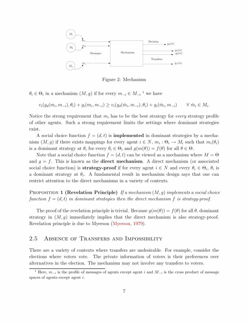
A mechanism is a pair (M, g), where M = M1 × . . . × Mn is the cross product of

message spaces of agents and g is a mapping g : M → D × Rn. The mapping g is called

an outcome function. For every profile of messages m = (m1, . . . , mn) ∈ M , the outcome

function g(m) = (gd(m), g1(m), . . . , gn(m)) gives a decision gd(m) ∈ D and a transfer gi(m)

to every agent i ∈ N . Hence, a mechanism is more general than a social choice function.

In a social choice function, the input is types of agents (for example, values of bidders in

an auction) but in a mechanism it is messages from agents. A message can be anything

arbitrary. For example, in an auction setting it can be a sequence of bounds on the value of

a bidder. The output of a mechanism and a social choice function is the same - a decision

and a vector of transfers. Clearly, a social choice function is also a mechanism where the

messages are restricted to be types only. This will be discussed later. Figure 2 gives a

pictorial description of a mechanism.

Notice the difference between a mechanism, often referred to as a game form, and a

game. An outcome in a mechanism is a decision and a vector of transfers but not a vector

of payoffs (as in a game). Of course, once the types and utility functions of all agents are

specified, it induces a game.

The goal of mechanism design is to design the message space and outcome function in a

way such that when agents participate in the mechanism they have (best) strategies (mes-

sages) that they can choose as a function of their private types such that the desired outcome

is achieved. The most fundamental, though somewhat demanding, notion in mechanism de-

sign is the notion of dominant strategies. A strategy mi ∈ Mi is a dominant strategy at

6

Mechanism

m1

m2

mn

gd(m)

g1(m)g2(m)

gn(m)

M1

M2

Mn

Messages

Decision

Transfers

Figure 2: Mechanism

θi ∈ Θi in a mechanism (M, g) if for every m−i ∈ M−i1 we have

vi(gd(mi, m−i), θi) + gi(mi, m−i) ≥ vi(gd(mi, m−i), θi) + gi(mi, m−i) ∀ mi ∈ Mi.

Notice the strong requirement that mi has to be the best strategy for every strategy profile

of other agents. Such a strong requirement limits the settings where dominant strategies

exist.

A social choice function f = (d, t) is implemented in dominant strategies by a mecha-

nism (M, g) if there exists mappings for every agent i ∈ N , mi : Θi → Mi such that mi(θi)

is a dominant strategy at θi for every θi ∈ Θi and g(m(θ)) = f(θ) for all θ ∈ Θ.

Note that a social choice function f = (d, t) can be viewed as a mechanism where M = Θ

and g = f . This is known as the direct mechanism. A direct mechanism (or associated

social choice function) is strategy-proof if for every agent i ∈ N and every θi ∈ Θi, θi is

a dominant strategy at θi. A fundamental result in mechanism design says that one can

restrict attention to the direct mechanisms in a variety of contexts.

Proposition 1 (Revelation Principle) If a mechanism (M, g) implements a social choice

function f = (d, t) in dominant strategies then the direct mechanism f is strategy-proof.

The proof of the revelation principle is trivial. Because g(m(θ)) = f(θ) for all θ, dominant

strategy in (M, g) immediately implies that the direct mechanism is also strategy-proof.

Revelation principle is due to Myerson (Myerson, 1979).

2.5 Absence of Transfers and Impossibility

There are a variety of contexts where transfers are undesirable. For example, consider the

elections where voters vote. The private information of voters is their preferences over

alternatives in the election. The mechanism may not involve any transfers to voters.

1 Here, m−i is the profile of messages of agents except agent i and M−i is the cross product of message

spaces of agents except agent i.

7

In such cases, one can restrict t to take value zero always and denote it as t0. Hence,

a decision rule d is strategy-proof if the social choice function (or direct mechanism) (d, t0)

is strategy-proof. Suppose D is finite. We say a type space is rich if for any ordering

ρ : D → 1, . . . , |D| and any i ∈ N , there exists a type θi ∈ Θi such that vi(d, θi) < vi(d, θ′i)

when ρ(d) < ρ(d′) for all d, d′ ∈ D. A decision rule d is dictatorial if there exists an

agent i ∈ N such that d(θ) ∈ arg maxd∈Rdvi(d, θi), where Rd = d ∈ D : there exists θ ∈

Θ with d(θ) = d is the range of the decision rule d. Dictatorial decision rules play a

pivotal role in mechanism design. It says that there exists a dictator agent whose utility is

maximized for every type profile of agents. For example, in the election set up, consider the

presence of a powerful voter who always decides who will be elected. Hence, types of agents

other than the dictator is disregarded by the mechanism. This is clearly a strategy-proof

social choice function, although not efficient. Unfortunately, this is the only strategy-proof

rule in many contexts.

Proposition 2 (Gibbard-Satterthwaite Impossibility) Suppose D is finite and the type

space is rich. A decision rule with at least three elements in its range is strategy-proof if and

only if it is dictatorial.

Proposition 2 was proved independently by Gibbard (1973) and Satterthwaite (1975) 2.

Though Proposition 2 is a very negative result, one need not lose hope. Proposition 2

critically relies on the assumptions made. There are social choice functions other than the

dictatorial one if one relaxes the richness of type space assumption or allow for transfers. For

example, under a class of type space called the single-peaked preferences, Moulin (1980)

shows the existence of a social choice function that is not dictatorial and has nice properties

(Pareto efficient, anonymous). As we will see next, in the context of auctions, we can get

many social choice functions that are strategy-proof by allowing for transfers.

2.6 Efficiency with Transfers

Here, I show a class of social choice functions which are strategy-proof and whose decision

rule is efficient. This is possible by allowing for transfers. These social choice functions are

famously known as the Groves mechanisms (Groves, 1973).

Proposition 3 (Groves Mechanisms) Suppose d is an efficient decision rule. For every

i ∈ N , let there be a function hi : Θ−i → R such that

ti(θ) = hi(θ−i) +∑

j∈N\i

vj(d(θ), θj) ∀ θ ∈ Θ.

Then (d, t) is strategy-proof.

2For an elegant and direct proof, see Sen (2001).

8

Before, I give a detailed proof, let us examine the transfer function of the Groves mechanism.

The first term in the transfer is a function, specific for every agent i, which depends on the

types of other agents but not on the type of i. The second term is the total value of agents

other than i in an efficient decision. We need to add the utility of agent i under efficient

decision to get the net utility i in a Groves mechanism. This will consist of a term which

is independent of his own type and the total welfare of agents in the efficient decision.

Intuitively, since efficient decision maximizes this net utility over all decisions, an agent

cannot get more net utility by deviating. This is the idea of the proof.

Proof : Suppose (d, t) is not strategy-proof. Then there exists an agent i ∈ N , θi ∈ Θi and

θ ∈ Θ such that

vi(d(θi, θ−i), θi) + ti(θi, θ−i) > vi(d(θ), θi) + ti(θ).

Expanding the ti(·) terms,

vi(d(θi, θ−i), θi) +∑

j 6=i

vj(d(θi, θ−i), θj) + hi(θ−i) > vi(d(θ), θi) +∑

j 6=i

vj(d(θ), θj) + hi(θ−i)

⇔∑

j∈N

vj(d(θi, θ−i), θj) >∑

j∈N

vj(d(θ), θj).

This contradicts efficiency. Hence, the Groves mechanism is strategy-proof.

Under some richness condition on type spaces, Groves mechanisms are the only mecha-

nisms that are efficient. 3 Hence, Groves mechanisms occupy a central role in mechanism

design.

A major drawback of Groves mechanism is that it is not balanced, a necessary requirement

in many public goods settings. To overcome this difficulty, researchers have resorted to weaker

notions of incentive compatibility, namely Bayesian incentive compatibility, which we will

examine later.

The Pivotal Mechanism

A particular mechanism in the class of Groves mechanism is intuitive and has many nice

properties (Moulin, 1986). It is commonly known as the pivotal mechanism or the Vickrey-

Clarke-Groves (VCG) mechanism (Vickrey, 1961; Clarke, 1971; Groves, 1973). The VCG

mechanism is characterized by a unique hi(·) function. In particular, for every agent i ∈ N

and every θ−i ∈ Θ−i, hi(θ−i) = −maxd∈D

∑

j 6=i vj(d, θj). This gives the following transfer

3Holmstrom (1979) shows that if the type space is smoothly connected then Groves mechanisms are the

only strategy-proof social choice functions that are efficient.

9

∅ 1 2 1, 2

v1(·) 0 8 6 12

v2(·) 0 9 4 14

Table 1: An Example of VCG Mechanism with Multiple Objects

function. For every i ∈ N and for every θ ∈ Θ, the transfer in the VCG mechanism is

ti(θ) =∑

j 6=i

vj(d(θ), θj) − maxd∈D

∑

j 6=i

vj(d, θj). (1)

A careful look at Equation 1 shows that the first term on the right hand side is the sum

of values of agents other than i in the efficient decision. The second term on the right hand

side is the maximum sum of values of agents other than i (note that this corresponds to an

efficient decision when agent i is excluded from the economy). Hence, negative of the transfer

in Equation 1 is the externality agent i inflicts on other agents because of his presence, and

this is the amount he pays. Thus, every agent pays his externality to other agents in the

VCG mechanism.

Consider the sale of a single object using the VCG mechanism. Fix an agent i ∈ N .

Efficiency says that the object must go to the bidder with the highest value. Consider the

two possible cases. In one case, bidder i has the highest value. So, when bidder i is present,

the sum of values of other bidders is zero (since no other bidder wins the object). But when

bidder i is absent, the maximum sum of value of other bidders is the second highest value

(this is achieved when the second highest value bidder is awarded the object). Hence, the

externality of bidder i is the second-higest value. In the case where bidder i ∈ N does

not have the highest value, his externality is zero. Hence, for the single object case, the

VCG mechanism is simple: award the object to the bidder with the highest (bid) value and

the winner pays the amount equal to the second highest (bid) value but other bidders pay

nothing. This is the well-known second-price auction or the Vickrey auction. By Proposition

3, it is strategy-proof.

We illustrate the VCG mechanism for the sale of multiple objects by an example. Consider

the sale of two objects, with values of two agents on bundles of goods given in Table 1. The

efficient allocation in this example is to give bidder 1 object 2 and bidder 2 object 1 (this

generates a total value of 6 + 9 = 15, which is higher than any other allocation). Let us

calculate the externality of bidder 1. The total value of bidders other than bidder 1, i.e.

bidder 2, in the efficient allocation is 9. When bidder 1 is removed, bidder 2 can get a

maximum value of 14 (when he gets both the objects). Hence, externality of bidder 1 is

14 − 9 = 5. Similarly, we can compute the externality of bidder 2 as 12− 6 = 6. Hence, the

payments of bidders 1 and 2 are 5 and 6 respectively.

10

2.7 Bayesian Incentive Compatibility

Bayesian incentive compatibility was introduced in Harsanyi (1967-68). It is a weaker re-

quirement than the dominant strategy incentive compatibility. While dominant strategy

incentive compatibility required the equilibrium strategy to be the best strategy under all

possible strategies of opponents, Bayesian incentive compatibility requires this to hold in

expectation. This means that in Bayesian incentive compatibility, an equilibrium strategy

must give the highest expected utility to the agent, where we take expectation over types

of other agents. To be able to take expectation, agents must have information about the

probability distributions from which types of other agents are drawn.

To understand Bayesian incentive compatibility, fix a mechanism (M, g). A Bayesian

strategy for such a mechanism is a vector of mappings mi : Θi → Mi for every i ∈ N . Notice

the difference from dominant strategy settings, where a message was a mapping from type

spaces of all agents to his own message space. A profile of such mapping m : Θ → M is a

Bayesian equilibrium if for all i ∈ N , for all θi ∈ Θi, and for all mi ∈ Mi we have

E−i

[

vi(gd(m−i(θ−i), mi(θi)), θi) + gi(m−i(θ−i), mi(θi))|θi

]

≥

E−i

[

vi(m−i(θ−i), mi) + gi(m−i(θ−i), mi)|θi

]

,

where E−i[·] denotes the expectation over type profile θ−i.

A dominant strategy incentive compatible mechanism is Bayesian incentive compatible.

A direct mechanism (social choice function) f = (d, t) is Bayesian incentive compatible

if mi(θi) = θi for all i ∈ N and for all θi ∈ Θi is a Bayesian equilibrium, i.e., for all i ∈ N

and for all θi, θi ∈ Θi we have

E−i

[

vi(d(θ−i, θi), θi) + gi(θ−i, θi)|θi

]

≥ E−i

[

vi(d(θ−i, θi), θi) + gi(θ−i, θi)|θi

]

A mechanism (M, g) realizes a social choice function f in Bayesian equilibrium if there

exists a Bayesian equilibrium m(·) of (M, g) such that g(m(θ)) = f(θ) for all θ ∈ Θ (that oc-

curs with positive probability). Analogous to the revelation principle for dominant strategy

incentive compatibility, we also have a revelation principle for Bayesian incentive compati-

bility.

Proposition 4 (Revelation Principle) If a mechanism (M, g) realizes a social choice

function f = (d, t) in Bayesian equilibrium, then the direct mechanism f = (d, t) is Bayesian

incentive compatible.

Again, the proof is trivial. It appears in Myerson (1979). It is one of the most widely used

concepts in mechanism design, and Myerson has used it in some of his other seminal work

(Myerson, 1981; Myerson and Satterthwaite, 1983). I will go into the details of Myerson

(1981), where he uses the revelation principle to design optimal auctions.

11

3 A Brief Summary of Contributions of Hurwicz

As noted earlier, Hurwicz is regarded as the founder of mechanism design. Hurwicz’s idea of

a mechanism is similar to what was discussed in the last section. According to Hurwicz, a

mechanism is like a machine which takes messages from agents, which may contain private

information of agents, and produces an outcome. Each agent is strategic, and tries to max-

imize his utility given a mechanism. This may force an agent to manipulate his messages,

and this creates the necessity that a mechanism be incentive compatible. He goes on to say

that different mechanisms wil produce different outcomes as equilibrium of these “message

games”, and the comparision of different mechanisms should be based on these equilibrium

outcomes.

Hurwicz elaborates these ideas in Hurwicz (1972). He also introduces the notion of

individual rationality - no agent should be made worse off by participating in a mechanism.

One of his seminal contributions, discussed in detail in Hurwicz (1972), is a negative result: in

a standard exchange economy, no strategy-proof mechanism satisfying individual rationality

can produce Pareto optimal outcomes.

The work of Hurwicz (1972) initiated the study of mechanism design. Researchers began

to ask several important questions that Huriwcz’s work had inspired. Here are some of those

questions, most of which have been answered. Can Pareto optimal outcomes be implemented

by considering a wider class of mechanisms? Can Pareto optimal outcomes be implemented

by weakening the notion of incentive compatibility? If answers to these questions are neg-

ative, then what is the worst loss of efficiency? What other objectives can be achieved if

efficiency cannot be achieved?

With the fundamental framework set by Hurwicz (1972), most of which was discussed in a

formal manner in Section 2, researchers began answering some of these questions. The work

of Myerson and Maskin are the most important answers to these questions. The revelation

principle theorem in Myerson (1979), the optimal auction design work in Myerson (1981),

and Nash implementation work of Maskin (Maskin, 1999) are examples of this. We elaborate

on these next.

4 Optimal Auction Design

This section will describe the design of optimal auction for selling a single indivisible object

to a set of bidders (buyers) who are risk neutral. The seminal paper in this area is (Myerson,

1981). We present a detailed analysis of this work 4, and point out some open questions

and ongoing research in this area. Before I describe the formal model, let me describe some

popular auction forms used in practice.

4An excellent treatment of the optimal auction design and related topics is (Krishna, 2002).

12

4.1 Auctions for a Single Indivisible Object

A single indivisible object is for sale. Let us consider four bidders (agents or buyers) who

are interested in buying the object. Let the valuations of the bidders be 10, 8, 6, and 4

respectively. I describe four commonly discussed auction formats using this example. As

before I assume risk neutral bidders with quasi-linear utility functions and private values.

• First-price auction: In the first-price auction, every bidder is asked to report a bid,

which indicates his value. The highest bidder wins the auction and pays the price he

bid. Of course, the bid amount need not equal the value. But if the bidders bid their

value, then the first bidder will win the object and pay an amount of 10.

• Second-price auction: In the second-price auction, like the first-price auction, each

bidder is asked to report a bid. The highest bidder wins the auction and pays the price

of the second highest bid. This is the Vickrey auction we have already discussed. As

we saw, a dominant strategy in this auction is that bidders will bid their values. Hence,

the first bidder will win the object but pay a price equal to 8, the second highest value.

• Dutch auction: The Dutch auction, popular for selling flowers in the Netherlands,

falls into a class of auctions called the open-cry auctions. The Dutch auction starts at

a high price and the price of the object is lowered by a small amount (called the bid

decrement) in iterations. In every iteration, bidders can express their interest to buy

the object. The price of the object is lowered only if no bidder shows interest. The

auction stops as soon as any bidder shows interest. The first bidder to show interest

wins the object at the current price.

In the example above, suppose the Dutch auction is started at price 12 and let the bid

decrement be 1. At price 12, no bidder should express interest since valuation of all

bidders are less than 12. After price 10, the first bidder may choose to express interest

since he starts getting non-negative utility from the object for any price less than or

equal to 10. If he chooses to express interest, then the auction would stop and he will

win the object. Clearly, it is not an equilibrium for the bidder to express interest at

10 since he can potentially get more payoff by waiting for the price to fall. Indeed, in

equilibrium (under some conditions), the bidder will show interest at a price just below

his valuation (see Krishna (2002) for details).

• English auction: The English auction is also an open-cry auction. The seller starts

the auction at a low price and raises it by a small amount (called the bid increment) in

iterations. In every iteration, like in the Dutch auction, the bidders are asked if they

are interested in buying the object. The price is raised only if more than one bidder

shows interest. The auction stops as soon as less than one bidder shows interest. The

last bidder to show interest wins the auction at the price he last showed interest.

13

In the example above, suppose the English auction is started at price 0 and let the bid

increment be 1. Then, at price 4 the bidder with value 4 will stop showing interest

(since he starts getting non-positive payoff from that price onwards). Similarly, at

prices 6, bidder with value 6 will drop out. Finally, bidder with value 8 will drop out

at price 8. At this price, only bidder with value 10 will show interest. Hence, the

auction will stop at price 8, and the bidder with value 10 will win the object at price 8.

Notice that the outcome of the auction is the same as the second-price auction. This is

no coincidence. It can be argued easily that it is an equilibrium (under private values

model) for bidders to show interest (bid) till the price reaches their value in the English

auction. Hence, the outcome of the English auction is the same as the second-price

auction.

One can think of many more auction formats - though they may not be used in practice.

Having learnt and thought about these auction formats, some natural questions arise. Is there

an equilibrium strategy for the bidder in each of these auctions? What kind of auctions are

incentive compatible? What is the ranking of these auctions in terms of expected revenue?

Which auction gives the maximum expected revenue to the seller over all possible auctions?

Myerson (1981) answers many of these questions. First, using the revelation principle (for

Bayesian incentive compatibility), he concludes that for every auction (sealed-bid or open-

cry or others) there exists a direct mechanism with the same social choice function, and thus

giving the same expected revenue to the seller. So, he focuses on direct mechanisms without

loss of generality. Second, he characterizes direct mechanisms which are Bayesian incentive

compatible. Third, he shows that all Bayesian incentive compatible mechanisms which have

the same allocation rule (e.g., the first-price auction and the second-price auction have the

same allocation rule since they both allocate the object to the bidder with the highest bid),

differ in revenue by a constant amount. Using these results, he is able to give a precise

description of an auction which gives the maximum expected revenue. He calls such an

auction an optimal auction. Under some conditions on the valuation distribution of bidders,

the optimal auction is a modified second-price auction. Next, we describe these results

formally.

4.2 The Model

There is a single indivisible object for sale, whose value for the seller is zero. The set of bidders

is denoted by N = 1, . . . , n. Every bidder has a value (this is his type) for the object. The

value of bidder i ∈ N is drawn from [0, hi] using a distribution with density function fi and

cumulative density Fi. We assume that each bidder draws his value independently and this

value is completely determined by this draw (i.e., knowledge of other information such as

value of other bidders does not influence his value). This model of valuation is referred to as

14

the private independent value model. We let the joint density function of values of all

the bidders as f and the joint density function of values of all the bidders except bidders i

as f−i. Due to the independence assumption,

f(x1, . . . , xn) = f1(x1) × . . . × fn(xn)

f(x1, . . . , xi−1, xi+1, . . . , xn) = f1(x1) × . . . × fi−1(xi−1) × fi+1(xi+1) × . . . fn(xn).

Let Xi = [0, hi] and X = [0, h1]× . . .× [0, hn]. Similarly, let X−i = ×j∈N\iXj. A typical

valuation of bidder i will be denoted as xi ∈ Xi, a valuation profile of bidders will be denoted

as x ∈ X, and a valuation profile of bidders in N \ i will be denoted as x−i ∈ X−i. The

valuation profile x = (x1, . . . , xi, . . . , xn) will sometimes be denoted as (xi, x−i). We assume

that fi(xi) > 0 for all i ∈ N and for all xi ∈ Xi.

4.3 The Direct Mechanism

Though a mechanism can be very complicated, a direct mechanism is simpler to describe.

By virtue of the revelation principle (Proposition 4), we can restrict attention to direct

mechanisms only. Henceforth, I will refer to a direct mechanism as simply a mechanism.

Let ∆ be the set of probability distributions over bidders in N . A mechanism M in

this context is a pair of mappings M = (a, p), where a : X → ∆ is the allocation rule

and p : X → Rn is the payment rule. Given a mechanism M = (a, p), a bidder i ∈ N

with (true) value xi ∈ Xi gets the following utility when all the buyers report values z =

(z1, . . . , zi, . . . , zn)

ui(z; xi) = ai(z)xi − pi(z).

Every mechanism (a, p) induces an expected allocation rule and an expected payment rule

(α, π), defined as follows. The expected allocation of bidder i when he reports zi ∈ Xi in

allocation rule a is

αi(zi) =

∫

X−i

ai(zi, z−i)f−i(z−i)dz−i.

Similarly, the expected payment of bidder i when he reports zi ∈ Xi in payment rule p is

πi(zi) =

∫

X−i

pi(zi, z−i)f−i(z−i)dz−i.

So, the expected utility from a mechanism (a, p) to a bidder i with true value xi by reporting

a value zi is αi(zi)xi − πi(zi).

Definition 1 A mechanism (a, p) is Bayesian incentive compatible if for every bidder

i ∈ N and for every possible true value xi ∈ Xi we have

αi(xi)xi − πi(xi) ≥ αi(zi)xi − πi(zi) ∀ zi ∈ Xi. (BIC)

15

Equation BIC says that a bidder maximizes his expected utility by reporting true value. So,

when bidder i has value xi, he gets more expected utility by reporting xi than by reporting

any other value zi ∈ Xi.

4.4 Characterization of Bayesian Incentive Compatibility

Myerson (1981) shows that Bayesian incentive compatibility is characterized by a special

class of allocation rules.

Definition 2 An allocation rule a is weakly monotone (w-mon) if for every bidder

i ∈ N and for every xi, zi ∈ Xi with xi > zi, we have αi(xi) ≥ αi(zi).

Theorem 1 (Incentive Comaptibility) For an allocation rule a, there exists a payment

rule p such that (a, p) is Bayesian incentive compatible if and only if αi(·) is w-mon for every

i ∈ N .

Proof : Suppose (a, p) is a Bayesian incentive compatible mechanism. Consider a buyer

i ∈ N and xi, zi ∈ Xi with xi > zi. Applying Equation BIC twice, we get

αi(xi)xi − πi(xi) ≥ αi(zi)xi − πi(zi)

αi(zi)zi − πi(zi) ≥ αi(xi)zi − πi(xi).

Adding these two equations, we get

αi(xi)xi + αi(zi)zi ≥ αi(zi)xi + αi(xi)zi

⇔[

αi(xi) − αi(zi)]

(xi − zi) ≥ 0.

Since xi > zi, this implies that αi(xi) ≥ αi(zi).

Now, suppose that a is w-mon. We will show that there exists a p such that (a, p) is

Bayesian incentive compatible. Consider a p whose expected payment is defined as follows.

For every i ∈ N and every xi ∈ Xi

πi(xi) = πi(0) + αi(xi)xi −

∫ xi

0

αi(ti)dti.

Since αi(·) is non-increasing, it is Riemann integrable, and hence, the above payment rule is

well defined. Now for any i ∈ N and any xi, zi ∈ Xi, we have

πi(xi) − πi(zi) = αi(xi)xi −

∫ xi

0

αi(ti)dti − αi(zi)zi +

∫ zi

0

αi(ti)dti

= αi(xi)xi − αi(zi)xi + αi(zi)xi − αi(zi)zi +

∫ zi

xi

αi(ti)dti

= αi(xi)xi − αi(zi)xi + αi(zi)(xi − zi) −

∫ xi

zi

αi(ti)dti.

16

αi(·)

xi zi

αi(zi)

αi(xi)

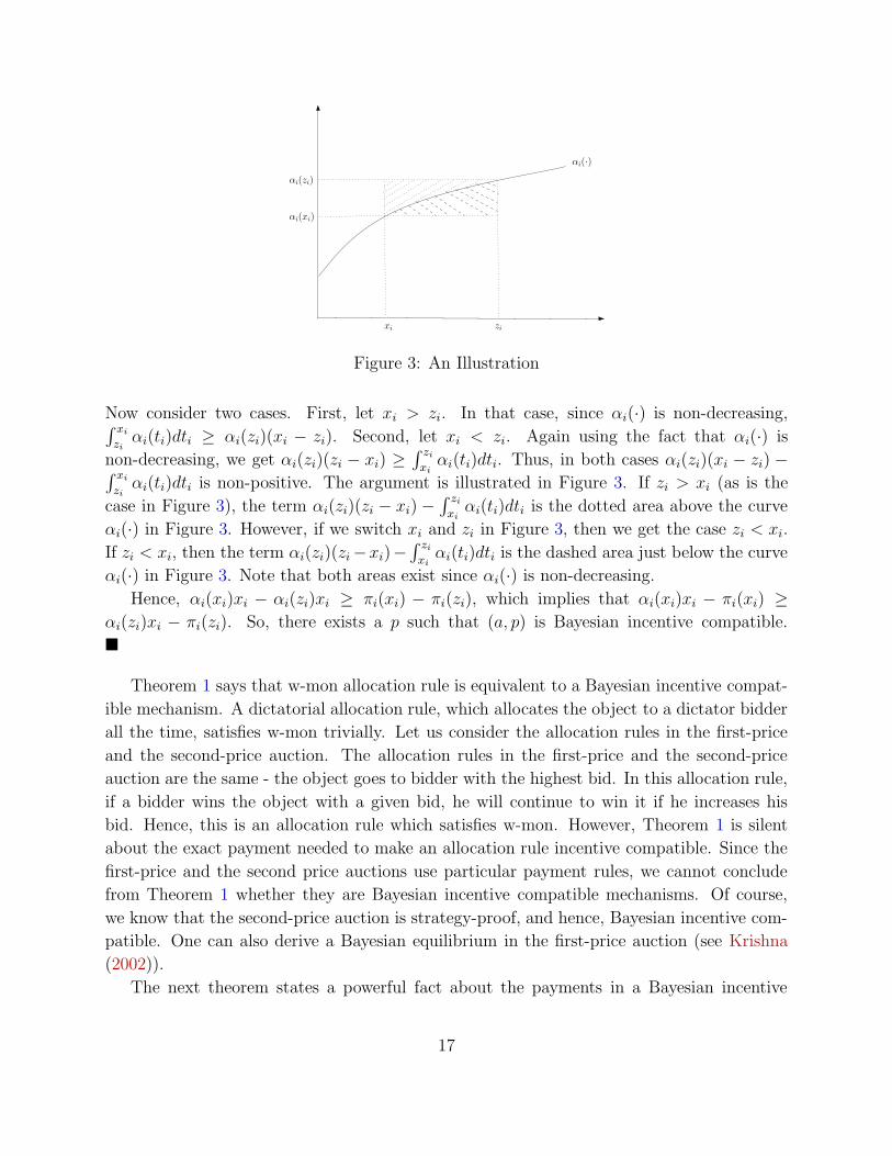
Figure 3: An Illustration

Now consider two cases. First, let xi > zi. In that case, since αi(·) is non-decreasing,∫ xi

zi

αi(ti)dti ≥ αi(zi)(xi − zi). Second, let xi < zi. Again using the fact that αi(·) is

non-decreasing, we get αi(zi)(zi − xi) ≥∫ zi

xi

αi(ti)dti. Thus, in both cases αi(zi)(xi − zi) −∫ xi

zi

αi(ti)dti is non-positive. The argument is illustrated in Figure 3. If zi > xi (as is the

case in Figure 3), the term αi(zi)(zi − xi) −∫ zi

xi

αi(ti)dti is the dotted area above the curve

αi(·) in Figure 3. However, if we switch xi and zi in Figure 3, then we get the case zi < xi.

If zi < xi, then the term αi(zi)(zi −xi)−∫ zi

xi

αi(ti)dti is the dashed area just below the curve

αi(·) in Figure 3. Note that both areas exist since αi(·) is non-decreasing.

Hence, αi(xi)xi − αi(zi)xi ≥ πi(xi) − πi(zi), which implies that αi(xi)xi − πi(xi) ≥

αi(zi)xi − πi(zi). So, there exists a p such that (a, p) is Bayesian incentive compatible.

Theorem 1 says that w-mon allocation rule is equivalent to a Bayesian incentive compat-

ible mechanism. A dictatorial allocation rule, which allocates the object to a dictator bidder

all the time, satisfies w-mon trivially. Let us consider the allocation rules in the first-price

and the second-price auction. The allocation rules in the first-price and the second-price

auction are the same - the object goes to bidder with the highest bid. In this allocation rule,

if a bidder wins the object with a given bid, he will continue to win it if he increases his

bid. Hence, this is an allocation rule which satisfies w-mon. However, Theorem 1 is silent

about the exact payment needed to make an allocation rule incentive compatible. Since the

first-price and the second price auctions use particular payment rules, we cannot conclude

from Theorem 1 whether they are Bayesian incentive compatible mechanisms. Of course,

we know that the second-price auction is strategy-proof, and hence, Bayesian incentive com-

patible. One can also derive a Bayesian equilibrium in the first-price auction (see Krishna

(2002)).

The next theorem states a powerful fact about the payments in a Bayesian incentive

17

compatible mechanism. It says that once we fix a w-mon allocation rule, the payment rule is

uniquely determined upto an additive constant. This is known as the revenue equivalence

result, and proved in Myerson (1981).

Theorem 2 (Revenue Equivalence) Suppose (a, p) is Bayesian incentive compatible. Then,

for every bidder i ∈ N and every xi ∈ Xi we have

πi(xi) = πi(0) + αi(xi)xi −

∫ xi

0

αi(ti)dti.

Proof : For every i ∈ N and every xi ∈ Xi denote Ui(xi) = αi(xi)xi − πi(xi). Consider a

bidder i ∈ N and xi, zi ∈ Xi. Since (a, p) is Bayesian incentive compatible, we can write

Ui(xi) ≥ αi(zi)xi − πi(zi)

= αi(zi)(xi − zi) + αi(zi)zi − πi(zi)

= Ui(zi) + αi(zi)(xi − zi).

Switching the role of xi and zi we get

Ui(zi) ≥ Ui(xi) + αi(xi)(zi − xi).

Hence, we can write

αi(xi)(zi − xi) ≤ Ui(zi) − Ui(xi) ≤ αi(zi)(zi − xi).

Let zi = xi + δ for δ > 0. Then, we get

αi(xi)δ ≤ Ui(xi + δ) − Ui(xi) ≤ αi(xi + δ)δ.

Hence, αi(·) is the derivative of Ui(·). Using the fundamental theorem of calculus, and the

fact that αi(·) is Riemann integrable since it is non-decreasing, we can write

∫ xi

0

αi(ti)dti = Ui(xi) − Ui(0).

Substituting Ui(0) = −πi(0) and Ui(xi) = αi(xi)xi − πi(xi), we get

∫ xi

0

αi(ti)dti = αi(xi)xi − πi(xi) + πi(0).

This gives us the desired inequality

πi(xi) = πi(0) + αi(xi)xi −

∫ xi

0

αi(ti)dti.

18

Theorem 2 says that the (expected) payment of a bidder in a mechanism is uniquely

determined by the allocation rule once we fix the expected payment of a bidder with the

lowest type. Hence, a mechanism is uniquely determined by its allocation rule and the

payment of a bidder with the lowest type. Suppose the payment to the lowest type is always

zero. Then, by Theorem 2, the expected revenue in the first-price and the second-price

auction (ad hence the English auction) is the same. This remarkable result hinges on the

assumptions we made earlier. For example, if we drop the assumption of private values and

allow a particular kind of interdependent valuation (value of every bidder depends on the

information of other bidders), then the English auction generates more expected revenue than

the second-price auction, which in turn generates more expected revenue than the first-price

auction. Similarly, if bidders are risk-averse then the expected revenue ranking of popular

auction formats change (Maskin and Riley, 1984).

We next impose a condition on the mechanism which determines the payment of a bidder

when he has the lowest type.

Definition 3 A mechanism (a, p) is individually rational if for every bidder i ∈ N we

have αi(xi)xi − πi(xi) ≥ 0 for all xi ∈ Xi.

Notice that if (a, p) is Bayesian incentive compatible and individually rational, then

πi(0) ≤ 0 for all i ∈ N . Note that if αi(·) is non-decreasing, then αi(xi) −∫ xi

0αi(ti)dti ≥ 0.

Hence, if πi(0) = 0, then πi(xi) ≥ 0 for all xi ∈ Xi. As we will see, the optimal auction has

πi(0) = 0, and thus πi(xi) ≥ 0 for all xi ∈ Xi, i.e., biddders pay the auctioneer. This is a

standard feature of auctions in practice where bidders are never paid.

4.5 Optimal Mechanism

Denote the expected revenue from a mechanism (a, p) as

Π(a, p) =∑

i∈M

∫ hi

0

πi(xi)f(xi)dxi.

We say a mechanism (a, p) is an optimal mechanism if

• (a, p) is Bayesian incentive compatible and individually rational,

• and Π(a, p) ≥ Π(a′, p′) for any other Bayesian incentive compatible and individually

rational mechanism (a′, p′).

19

Fix a mechanism (a, p) which is Bayesian incentive compatible and individually rational.

For any bidder i ∈ N , the expected payment of bidder i ∈ N is given by

∫ hi

0

πi(xi)f(xi)dxi = πi(0) +

∫ hi

0

αi(xi)xif(xi)dxi −

∫ hi

0

∫ xi

0

(

αi(ti)dti)

f(xi)dxi,

where the last equality comes by using revenue equivalence (Theorem 2). By interchanging

the order of integration in the last term, we get

∫ hi

0

∫ xi

0

(

αi(ti)dti)

f(xi)dxi =

∫ hi

0

(

∫ hi

ti

f(xi)dxi

)

αi(ti)dti

=

∫ hi

0

(1 − Fi(ti))αi(ti)dti.

Hence, we can write

Π(a, p) =∑

i∈N

πi(0) +∑

i∈N

∫ hi

0

(

xi −1 − Fi(xi)

fi(xi)

)

αi(xi)fi(xi)dxi.

We now define the virtual valuation of bidder i ∈ N with valuation xi ∈ Xi as

vi(xi) = xi −1 − Fi(xi)

fi(xi).

Note that since fi(xi) > 0 for all i ∈ N and for all xi ∈ Xi, the virtual valuation vi(xi) is

well defined. Also, not that virtual valuations can be negative. Using this and the definition

of αi(·), we can write

Π(a, p) =∑

i∈N

πi(0) +∑

i∈N

∫ hi

0

vi(xi)αi(xi)fi(xi)dxi

=∑

i∈N

πi(0) +∑

i∈N

∫ hi

0

(

∫

X−i

ai(xi, x−i)f−i(x−i)dx−i

)

vi(xi)fi(xi)dxi

=∑

i∈N

πi(0) +∑

i∈N

∫

X

vi(xi)ai(x)f(x)dx

=∑

i∈N

πi(0) +

∫

X

(

∑

i∈N

vi(xi)ai(x))

f(x)dx.

We need to maximize Π(a, p) subject to Bayesian incentive compatibility and individual

rationality constraints. Let us sidestep Bayesian incentive compatibility constraint for the

moment. So, we are only concerned about maximizing

Π(a, p) =∑

i∈N

πi(0) +

∫

X

(

∑

i∈N

vi(xi)ai(x))

f(x)dx, (2)

20

subject to individual rationality constraint. But individual rationality says πi(0) ≤ 0 for all

i ∈ N . Hence, if we want to maximize Π(a, p), then πi(0) = 0 for all i ∈ N . A careful look

at the second term on the right hand side of Equation 2 is necessary. Consider a profile

of valuations x ∈ X. Consider∑

i∈N vi(xi)ai(x) for a valuation profile x ∈ X. This is

maximized by setting ai(x) = 1 if vi(xi) = maxj∈N vj(xj) ≥ 0, else setting ai(x) = 0 for all

i ∈ N . That is, we allocate the object to the buyer with the highest non-negative virtual

valuation, and we do not allocate the object if the highest virtual valuation is negative. This

way, we will maximize∑

i∈N vi(xi)ai(x), and hence will maximize∑

i∈N vi(xi)ai(x)f(x). This

in turn will maximize the second term on the right hand side of Equation 2.

Now, we come back to Bayesian incentive compatibility requirement. By virtue of The-

orem 1, we need to ensure that the suggested allocation rule is w-mon. In general, it is not

w-mon. However, it is w-mon under the following condition. We say the regularity condi-

tion holds if for every bidder i ∈ N , vi(xi) ≥ vi(zi) for all xi, zi ∈ Xi with xi > zi. In other

words, for all i ∈ N , for all xi, zi ∈ Xi with xi > zi, regularity is satisfied if 1−Fi(xi)fi(xi)

≤ 1−Fi(zi)fi(zi)

.

The term fi(xi)1−Fi(xi)

is called the hazard rate. So, regularity is satisfied if the hazard rate is

non-decreasing. The uniform distribution satisfies the regularity condition.

If the regularity condition holds, then a is w-mon. To see this, consider a bidder i ∈ N

and xi, zi ∈ Xi with xi > zi. Regularity gives us vi(xi) ≥ vi(zi). By the definition of the

allocation rule, for all x−i ∈ X−i, we have ai(xi, x−i) ≥ ai(zi, x−i). Hence, a is w-mon. The

associated payment for bidder i ∈ N for a profile of valuation x can be computed from

Theorem 2 subject to the fact that πi(0) = 0.

pi(x) = ai(x)xi −

∫ xi

0

ai(ti, x−i)dti

This describes an optimal mechanism. From Equation 2 and the description of the opti-

mal mechanism, the expected highest revenue is the expected value of the highest virtual

valuation provided it is non-negative.

This mechanism can be simplified further. Define for all i ∈ N and all x−i ∈ X−i

qi(x−i) = infzi : vi(zi) ≥ 0 and vj(xj) ≤ vi(zi) ∀ j 6= i.

Hence, qi(x−i) is the valuation whose corresponding virtual valuation is non-negative and

“beats” the virtual valuations of other bidders. Thus the optimal allocation rule under

regularity condition can be rewritten as, for all i ∈ N , for all zi ∈ Xi, and for all x−i ∈ X−i,

ai(zi, x−i) = 1 if zi > qi(x−i)

ai(zi, x−i) = 0 otherwise.

21

Hence, for all i ∈ N , for all xi ∈ Xi, and for all x−i ∈ X−i

∫ xi

0

ai(zi, x−i)dzi = xi − qi(x−i) if xi > qi(x−i)

∫ xi

0

ai(zi, x−i)dzi = 0 otherwise.

This simplifies the payment rule. For all i ∈ N , for all xi ∈ Xi, and for all x−i ∈ X−i

pi(x) = qi(x−i) if ai(x) = 1

pi(x) = 0 if ai(x) = 0.

Thus, the optimal mechanism is the following auction. We order the virtual valuations of

bidders. Award the object to the highest non-negative virtual valuation bidder (breaking ties

arbitrarily - ties will happen with probability zero), and the winner, if any, pays the valuation

corresponding to the second highest virtual valuation, while the losers pay nothing. In other

words, the seller sets a reserve price 5 equal to maxi∈N v−1i (0) and for the valuations that

exceed this reserve price, he conducts the above auction. This leads to the seminal result in

(Myerson, 1981).

Theorem 3 (Optimal Auction) Suppose the regularity condition holds. Then, the fol-

lowing mechanism is optimal. For all i ∈ N ,

ai(x) = 1 if vi(xi) > maxj 6=i

vj(xj) and vi(xi) ≥ 0

ai(x) = 0 otherwise

pi(x) = qi(x−i) if ai(x) = 1

pi(x) = 0 if ai(x) = 0.

Finally, we look at the special case where the buyers are symmetric, i.e., they draw

the valuations using the same distribution - fi = f for all i ∈ N . So, virtual valuations

are the same: vi = v for all i ∈ N . Hence, maximum virtual valuation corresponds to the

maximum valuation. Thus, qi(x−i) = maxv−1(0), maxj 6=i xj. This is exactly, the second-

price auction with the reserve price of v−1(0). Hence, when the buyers are symmetric, then

the second-price auction with a reserve price is optimal. Typically, the optimal mechanism

is inefficient.

Though the second-price auction is rarely used in practice, but is weakly equivalent to the

popular English auction. Under regularity and symmetric bidders, the optimal mechanism

can be implemented using an English auction. The auction starts at price v−1(0) and the

price is raised till exactly one bidder is interested in the object.

5A reserve price in an auction indicates that if bids are less than the reserve price than the object will

not be sold.

22

4.6 Extensions of Myerson’s Optimal Auction Work

The contribution in Myerson (1981) has been extended in many directions. In the single

object case, several authors have tried to extend the results in Myerson (1981) by relaxing

some of the assumptions and putting more qualifications in the auction design. For example,

by relaxing the independent private value assumption, Cremer and McLean (1988) show that

a slight degree of correlation allows the seller to extract the entire surplus from the bidders,

i.e., expected payoff of every bidder can be made zero 6. For a full account of results on

the extensions of Myerson (1981) and other topics in single object auction, the readers are

directed to Krishna (2002).

We discuss some recent extensions to the multi-object auction case. To do so, let us first

examine the complexity of the multi-object model. In a multi-object model, there is a set

of objects M = 1, . . . , m. The objects can be homogeneous or heterogeneous. A bidder

i ∈ N has a valuation function vi : 2M → R+, i.e., for every bundle of objects S ⊆ M ,

bidder i ∈ N associates a value vi(S). Thus, the value of a buyer is multi-dimensional. The

multi-dimensional nature of the problem creates challenges. It is not clear whether Theorems

1 and 2 extend to the multi-dimensional case.

To describe the multi-dimensional problem, for every agent i ∈ N , his type space is k

dimensional, i.e., Xi ⊆ Rk. Let A be a finite set of outcomes. Let vi : A × Xi → R be

the valuation function of agent i ∈ N . As before X = ×i∈NXi and X−i = ×j 6=iXj. An

allocation rule a is a mapping a : X → A. A payment rule p is a mapping p : X → R. A

mechanism (a, p) is dominant strategy incentive compatible if for every agent i ∈ N ,

every x−i ∈ X−i, and every xi, zi ∈ Xi we have

vi(a(x), xi) − pi(x) ≥ vi(a(zi, x−i), xi) − pi(zi, x−i)

Writing this constraint by switching the roles of xi and zi, and adding these two equations

we get the following necessary condition for dominant strategy incentive compatibility. For

every agent i ∈ N and for every x−i ∈ X−i we need

[

vi(a(xi, x−i), xi) − vi(a(zi, x−i), xi)]

+[

vi(a(zi, x−i), zi) − vi(a(xi, x−i), zi)]

≥ 0. (3)

Condition in Equation 3 is referred to as the weak monotonicity (wmon) condition for

multi-dimensional types 7. As was shown, this is clearly a necessary condition for incentive

compatibility. For a variety of domains (i.e., restriction on X), this is also sufficient.

Some ongoing research has focused on extending the w-mon characterization to multi-

object auctions. The extensions of w-mon characterizations are mainly for dominant strat-

6Cremer and McLean (1988) make the assumption that valuations are drawn from a discrete distribution,

a condition called the single crossing is satisfied, and the matrix of beliefs has full rank.7An obvious modification in notation gives an equivalent condition for Bayesian incentive compatibility.

23

egy incentive compatibility, except Muller et al. (2007). As long as the closure of the do-

main of valuations is convex, w-mon is necessary and sufficient for dominant strategy in-

centive compatibility in the multi-object case, as is shown in Monderer (2007) 8. Other

notable extensions of Theorem 1 to multi-dimensional case are Bikhchandani et al. (2006),

Saks and Wu (2005), Muller et al. (2007) (they characterize Bayesian incentive compatibil-

ity), and Gui et al. (2004).

The revenue equivalence result of Theorem 2 have also been extended to the multi-

dimensional case. Hydenreich et al. (2007) give a directed graph interpretation of the incen-

tive compatibility constraints, and use it to characterize multi-dimensional domains where

revenue equivalence holds. Other notable extensions of Theorem 2 are Milgrom and Segal

(2002), Krishna and Maenner (2001), and Chung and Olszewski (2007).

The optimal auction design problem for the multi-object case is still an open problem.

Armstrong (2000) analyzes this problem for two objects case when buyers valuations are

additive (i.e., value for a bundle of object is sum of values of objects in the bundle). When

values are drawn from a binary distribution, they construct optimal auctions under some

technical conditions on the distributions of the bidders. His work shows the difficulty in-

volved in solving the problem. Recent work by Malakhov and Vohra (2008), again assuming

discrete distribution of valuations of bidders, using directed graph interpretation of incen-

tive compatibility constraints make some advance in the multi-dimensional optimal auction

design. However, a general solution still alludes the literature.

5 Nash Implementation

In this section, we briefly describe an important contribution of Eric Maskin. In order to do

so, we first give a general setting for implementation. Then, we describe the seminal results

on Nash implementation of Maskin (1999). For a detailed discussion on implementation, see

Jackson (2001). Jackson (2001) is also an excellent place to know about the contributions

of Leonid Hurwicz.

Having discussed the mechanism design setting, the implementation setting differs from

it in one major way. In the implementation setting, the agents know each others preferences

(complete information setting). However, the designer does not know the preferences of

the agents. This is still a useful setting for many situations. Consider a situation where

a firm and one of his suppliers are in a dispute about the quality of the good supplied by

the supplier. They decide to take the dispute to a regulatory authority. The firm and his

supplier are aware of the actual quality of the goods supplied, but the regulator is not aware

of the quality. What mechanism can the regulator design to elicit true information from the

8Monderer (2007) also shows that any domain of valuations where w-mon allocation rule characterizes

incentive compatibility must be a domain whose closure is convex.

24

supplier and the firm? The implementation literature answers such questions.

5.1 The Model

As before N = 1, . . . , n denotes a finite set of agents. The set of outcomes is denoted by

A, which can be finite or infinite. The set of outcomes is an arbitrary set. Let Ω = S ⊆

A : S 6= ∅. The preference of agent i is represented by a binary relation Ri over A which

is complete and transitive. We let aRib for any a, b ∈ A to denote that a is at least as good

as b for agent i. The strict preference associated with a binary relation Ri is denoted as Pi.

We use the standard notation R to denote a profile of binary relations and R−i to denote a

profile of binary relations of agents other than agent i. The set of all admissible preference

profiles is P.

A social choice correspondence F is a mapping F : P → Ω. So, for a profile of

preferences R ∈ P, F (R) represents the desirable set of alternatives. We say F (·) is a social

choice function if it is single-valued.

As before, a mechanism is a pair (M, g), where M is the product of message spaces of

agents and g is the outcome function g : M → A. A message profile m is a Nash equilib-

rium of a mechanism (M, g) at preference profile R if for every i ∈ N , gi(mi, m−i)Rigi(m′i, m−i)

for all m′i ∈ Mi. Let NEΓ(R) ⊆ M denote the set of Nash equilibria of mechanism Γ = (M, g)

at preference profile R. Let g(NEΓ(R)) = a ∈ A : a = g(m) for some m ∈ NEΓ(R) be

the set of outcomes obtained in Nash equilibrium of mechanism Γ at preference profile R.

A social choice correspondence F is implemented by the mechanism Γ = (M, g) in Nash

equilibrium if g(NEΓ(R)) = F (R) for all R ∈ P. A social choice correspondence F is said to

be implementable in Nash equilibrium if there exists a mechanism (M, g) which implements

it.

5.2 Nash Implementation and Monotonicity

The seminal work of Maskin (1999) not only gives us necessary and sufficient conditions for

Nash implementable social choice correspondences but also provides a technique, which is

extensively used in subsequent literature.

The condition identified by Maskin is a monotonicity condition which is necessary for

Nash implementation. Suppose a social choice correspondence F is Nash implementable by

a mechanism (M, g). Consider a preference profile R and let F (R) = a. So, there exists

m ∈ M such that g(m) = a and m is a Nash equilibrium at R. Now, suppose there exists

another preference profile R′ such that a /∈ F (R′). Since F is Nash implementable by (M, g),

this implies that m is not a Nash equilibrium, and there exists an agent i and a message

25

m′i ∈ Mi such that

g(m′i, m−i)P

′ig(mi, m−i).

Since m was a Nash equilibrium at R we can write

g(mi, m−i)Rig(m′i, m−i)

If we let b = g(m′i, m−i), we get bP ′

i a and aRib. Thus, we have arrived at a necessary

condition for Nash implementation.

Definition 4 A social choice correspondence F is Maskin monotonic if for every R, R′ ∈

P and every a ∈ F (R) \ F (R′), there exists i ∈ N and b ∈ A such that bP ′i a and aRib.

Maskin monotonicity says that if some alternative is in the social choice correspondence

at a profile but not in another profile, then it must have fallen in some agent’s preference

ranking (to break the Nash equilibrium). By our arguments earlier, the following theorem is

immediate, which was proved in Maskin (1999).

Theorem 4 (Necessity of Monotonicity) If a social choice correspondence is Nash im-

plementable, then it is Maskin monotonic.

There is an equivalent way to state Maskin monotonicity. Consider a profile R and

a ∈ F (R). Consider R′ such that for each i ∈ N we have aRib implies aR′ib, i.e., ranking of a

in i’s preference has not fallen from R to R′. Since F is Nash implementable by (M, g), there

exists m ∈ M such that g(mi, m−i)Rig(m′i, m−i) for all m′

i ∈ Mi, where g(mi, m−i) = a. But

for each b such that aRib we have aR′ib. Hence, g(mi, m−i)R

′ig(m′

i, m−i) for all i ∈ N and for

all m′i ∈ Mi. Hence, m is also a Nash equilibrium at R′, i.e., a ∈ F (R′). So, an equivalent

statement of Maskin monotonicity is the following. A social choice correspondence F is

Maskin monotonic if for any R and a ∈ F (R) and for R′ such that aRib implies that aR′ib

for all i ∈ N , we have a ∈ F (R′).

While Maskin monotonicity is necessary for Nash implementation, we need more sufficient

conditions for Nash implementation. When n ≥ 3, Maskin (1999) shows that monotonicity

along with a condition called no veto power is sufficient for Nash implementation.

Definition 5 A social choice correspondence satisfies no veto power if whenever i, R,

and a are such that aRjb for all j 6= i and all b ∈ A, we have a ∈ F (R).

Clearly, no veto power is very restrictive when there are two agents. Maskin (1999)

proved the following.

Theorem 5 (Sufficiency) Suppose n ≥ 3. If a social choice correspondence satisfies

Maskin monotonicity and no veto power, then it is Nash implementable.

We omit the proof, but note that the proof is constructive. For every social choice corre-

spondence F satisfying Maskin monotonicity and no veto power, Maskin (1999) constructs

a mechanism which implements it.

26

5.3 Extensions

Maskin’s original work was circulated as a discussion paper in 1977, and it started a flurry of

extensions. For n = 2, the sufficiency result in Maskin (1999) does not work. Dutta and Sen

(1991) provide a sufficient condition for the n = 2 case. Researchers have also studied the

consequence of other kinds of solution concepts for implementation. Virtual (approximate)

implementation is studied in Matsushima (1988); Abreu and Sen (1991), implementation

by sequential mechanisms is studied in Moore and Repullo (1988); Abreu and Sen (1990),

and implementation in (incomplete information settings) Bayesian equilibrium is studied

in Dutta and Sen (1994). Several new solution concepts of equilibrium have since been

proposed, and researchers continue to find mechanisms that can be implemented in these

new solution concepts. For details, the reader is referred to Jackson (2001).

6 Conclusion

Two surveys by Jackson (2001, 2003) have more details on the topic of implementation and

mechanism design. The present survey is more succinct than these surveys. I focused on

the foundations of mechanism design and went into the details of Myerson’s optimal auction

design work. I specially highlighted some of the extensions and ongoing research of Myerson’s

work. I also touched on, though briefly, the implementation setting and Maskin’s seminal

Nash implementation work.

Another place to learn about the contributions of 2007 economics Nobel prize winners

is the scientific background document compiled by the Prize committee of Royal Swedish

Academy of Sciences titled “Mechanism Design Theory” (it can be accessed on the Internet

web site of Nobel Prize: http://nobelprize.org). This scientific background document

gives an overview of all the major contributions of the three laureates.

The applications of mechanism design theory is growing. With the advent of Internet,

new types of markets are being created. This is generating new fundamental questions in

mechanism design theory, and mechanism design theory is being applied in many new areas

(some of which we discussed in Section 1.1). These applications owe their success to the

sound theory of mechanism design, foundations of which were laid by Hurwicz, Maskin, and

Myerson.

References

Abreu, D. and A. Sen (1990): “Implementation in Subgame Perfect Equilibrium: A

Necessary and Almost Sufficient Condition,” Journal of Economic Theory, 50, 285–299.

——— (1991): “Virtual Implementation in Nash Equilibrium,” Econometrica, 59, 997–1021.

27

Armstrong, M. (2000): “Optimal Multi-Object Auctions,” Review of Economic Studies,

67, 455–481.

Bikhchandani, S., S. Chatterji, R. Lavi, A. Mualem, N. Nisan, and A. Sen

(2006): “Weak Monotonicity Characterizes Deterministic Dominant Strategy Implemen-

tation,” Econometrica, 74, 1109–1133.

Chung, K. and W. Olszewski (2007): “A Non-Differentiable Approach to Revenue

Equivalence,” Theoretical Economics, 2, 469–487.

Clarke, E. (1971): “Multipart Pricing of Public Goods,” Public Choice, 8, 19–33.

Cramton, P. (2002): “Spectrum Auctions,” in Handbook of Telecommunications Eco-

nomics, ed. by M. Cave, S. Majumdar, and I. Vogelsang, Amsterdam: Elsevier Science,

605–639.

Cramton, P., Y. Shoham, and R. S. (Editors) (2006): Combinatorial Auctions, MIT

Press.

Cremer, J. and R. McLean (1988): “Full Surplus Extraction of the Surplus in Bayesian

and Dominant Strategy Auctions,” Econometrica, 56, 1247–1257.

Dutta, B. and A. Sen (1991): “Necessary and Sufficient Conditions for 2 Person Nash

Implementation,” Review of Economic Studies, 121–129.

——— (1994): “Bayesian Implementation: The Necessity of Infinite Mechanisms,” Journal

of Economic Theory, 130–141.

Edelman, B., M. Ostrovsky, and M. Schwarz (2007): “Internet Advertising and

the Generalized Second Price Auction: Selling Billions of Dollars Worth of Keywords,”

American Economic Review, 97, 242–259.

Gibbard, A. (1973): “Manipulation of Voting Schemes: A General Result,” Econometrica,

41, 587–601.

Groves, T. (1973): “Incentives in Teams,” Econometrica, 41, 617–663.

Gui, H., R. Muller, and R. V. Vohra (2004): “Characterizing Dominant Strategy

Mechanisms with Multi-Dimensional Types,” Tech. rep., Kellogg School of Management,

Northwestern University.

Harsanyi, J. C. (1967-68): “Games of Incomplete Information Played by ‘Bayesian’ Play-

ers,” Management Science, 14, 159–189, 320–334, 486–502.

28

Holmstrom, B. (1979): “Groves Scheme on Restricted Domain,” Econometrica, 47, 1137–

1147.

Hurwicz, L. (1972): “On Informationally Decentralized Systems,” in Decisions and Orga-

nizations, ed. by Radner and McGuire, North-Holland, Amsterdam.

Hydenreich, B., R. Muller, M. Uetz, and R. V. Vohra (2007): “Characteriza-

tion of Revenue Equivalence,” Tech. rep., Kellogg School of Management, Northwestern

University.

Jackson, M. (2001): “A Crash Course in Implementation Theory,” Social Choice and Wel-

fare, 18, 655–708.

——— (2003): “Mechanism Theory,” in Encyclopedia of Life Support Systems, ed. by U. De-

rigs, EOLSS Publishers.

Krishna, V. (2002): Auction Theory, Acamdemic Press.

Krishna, V. and E. Maenner (2001): “Convex Potentials with an Application to Mech-

anism Design,” Econometrica, 69, 1113–1119.

Malakhov, A. and R. V. Vohra (2008): “An Optimal Auction for Capacity Constrained

Bidders: A Network Perspective,” Economic Theory, Forthcoming.

Maskin, E. (1999): “Nash Equilibrium and Welfare Optimality,”Review of Economic Stud-

ies, 66, 23–38.

Maskin, E. and J. Riley (1984): “Optimal Auctions with Risk-Averse Buyers,” Econo-

metrica, 54, 1473–1518.

Matsushima, H. (1988): “A New Approach to the Implementation Problem,” Journal of

Economic Theory, 45, 128–144.

Milgrom, P. and I. Segal (2002): “Envelope Theorems with Arbitrary Choice Sets,”

Econometrica, 70, 583–601.

Monderer, D. (2007): “Monotonicity and Implementability,” Tech. rep., Technion Univer-

sity, Haifa.

Moore, J. and R. Repullo (1988): “Subgame Perfect Implementation,” Econometrica,

58, 1088–1100.

Moulin, H. (1980): “On Strategy-proofness and Single-Peakedness,” Public Choice, 35,

437–455.

29

——— (1986): “Characterizations of the Pivotal Mechanism,” Journal of Public Economics,

31, 53–78.

Muller, R., A. Perea, and S. Wolf (2007): “Weak Monotonicity and Bayes-Nash

Incentive Compatibility,” Games and Economic Behavior, 61, 344–358.

Myerson, R. B. (1979): “Incentive Compatibility and the Bargaining Problem,” Econo-

metrica, 47, 61–73.

——— (1981): “Optimal Auction Design,” Mathematics of Operations Research, 6, 58–73.

Myerson, R. B. and M. Satterthwaite (1983): “Efficient Mechanisms for Bilateral

Trading,” Journal of Economic Theory, 28, 265–281.

Nisan, N., T. Roughgarden, E. Tardos, and V. V. (Editors) (2007): Algorithmic

Game Theory, Cambridge University Press.

Saks, M. and L. Wu (2005): “Weak Monotonicity Suffices for Truthfulness on Convex

Domains,” in Proceedings of 6th Conference on Electronic Commerce, 286–293.

Satterthwaite, M. (1975): “Stategy-proofness and Arrow’ Conditions: Existence and

Correspondence Theorems for Voting Procedures and Social Welfare Theorems,” Journal

of Economic Theory, 10, 187–217.

Sen, A. (2001): “Another Direct Proof of the Gibbard-Sattrthwaite Theorem,” Economics

Letters, 70, 381–385.

Vickrey, W. (1961): “Counterspeculation, Auctions, and Competitive Sealed Tenders,”

Journal of Finance, 16, 8–37.

30