ECE 680 Fall 2017

An Introduction to Model-based PredictiveControl (MPC)

by

Stanislaw H. Zak

1 Introduction

The model-based predictive control (MPC) methodology is also referred to as the moving

horizon control or the receding horizon control. The idea behind this approach can be

explained using an example of driving a car. The driver looks at the road ahead of him and

taking into account the present state and the previous action predicts his action up to some

distance ahead, which we refer to as the prediction horizon. Based on the prediction, the

driver adjusts the driving direction. The MPC main idea is illustrated in Figure 1.

Y

Prediction horizon

X

vx

vy

vLane direction

Figure 1: The driver predicts future travel direction based on the current state of the car

and the current position of the steering wheel.

The MPC is constructed using control and optimization tools. The objective of this

write-up is to introduce the reader to the linear MPC which refers to the family of MPC

schemes in which linear models of the controlled objects are used in the control law synthesis.

c©2017 by Stanislaw H. Zak

1

In the MPC approach, the current control action is computed on-line rather than using

a pre-computed, off-line, control law.

A model predictive controller uses, at each sampling instant, the plant’s current input

and output measurements, the plant’s current state, and the plant’s model to

• calculate, over a finite horizon, a future control sequence that optimizes a given per-

formance index and satisfies constraints on the control action;

• use the first control in the sequence as the plant’s input.

The MPC strategy is illustrated in Figure 2, where Np is the prediction horizon, u(t+k|t) is

the predicted control action at t+ k given u(t). Similarly, y(t+ k|t) is the predicted output

at t+ k given y(t).

future/predictionpast

set-point

prediction horizon Np

ti ti + 1 ti + 2 ti + Np. . .

u(ti)

y(ti)u(ti + 2|ti)

y(ti + 2|ti)

Figure 2: Controller action construction using model-based predictive control (MPC) ap-

proach.

2 Basic Structure of MPC

In Figure 3, we show a basic structure of an MPC-controlled plant, where we assume that

the plant’s state is available to us.

3 From Continuous to Discrete Models

Our objective here is to present a method for constructing linear discrete-time models from

given linear continuous-time models. The obtained discrete models will be used to perform

2

Model Predictive Controller

cost function

u(ti) y(ti)+_

predictederror

predictedoutput

PlantModel

Optimizerpredicted

input Plantr( ).

x(ti)x

constraints

Figure 3: State feedback model predictive controller.

computations to generate control commands.

We use a sample-and-hold device that transforms a continuous signal, f(t), into the

staircase signal,

f(kh), kh ≤ t < (k + 1)h,

where h is the sampling period. The sample and zero-order hold (ZOH) operation is illus-

trated in Figure 4

f(t)

0

SampleandZOH

t t0

f(0)

f(2h)

f(h)

3h2hh

Figure 4: Sample and zero-order hold (ZOH) element operating on a continuous function.

Suppose that we are given a continuous-time model,

x(t) = Ax(t) +Bu(t), x0 = x(t0)

y(t) = Cx(t).

3

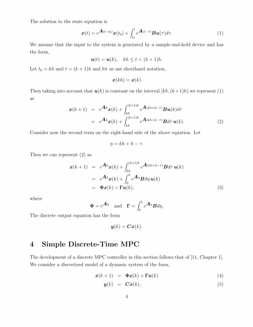
The solution to the state equation is

x(t) = eA(t−t0)x(t0) +∫ t

t0eA(t−τ)Bu(τ)dτ. (1)

We assume that the input to the system is generated by a sample-and-hold device and has

the form,

u(t) = u(k), kh ≤ t < (k + 1)h.

Let t0 = kh and t = (k + 1)h and let us use shorthand notation,

x(kh) = x(k)

Then taking into account that u(k) is constant on the interval [kh, (k+1)h) we represent (1)

as

x(k + 1) = eAhx(k) +∫ (k+1)h

kheA(kh+h−τ)Bu(k)dτ

= eAhx(k) +∫ (k+1)h

kheA(kh+h−τ)Bdτ u(k). (2)

Consider now the second term on the right-hand side of the above equation. Let

η = kh+ h− τ.

Then we can represent (2) as

x(k + 1) = eAhx(k) +∫ (k+1)h

kheA(kh+h−τ)Bdτ u(k)

= eAhx(k) +∫ h

0eAηBdηu(k)

= Φx(k) + Γu(k), (3)

where

Φ = eAh and Γ =∫ h

0eAηBdη.

The discrete output equation has the form

y(k) = Cx(k).

4 Simple Discrete-Time MPC

The development of a discrete MPC controller in this section follows that of [11, Chapter 1].

We consider a discretized model of a dynamic system of the form,

x(k + 1) = Φx(k) + Γu(k) (4)

y(k) = Cx(k), (5)

4

where Φ ∈ Rn×n, Γ ∈ Rn×m, and C ∈ Rp×n.

Applying the backward difference operator, ∆x(k + 1) = x(k + 1)− x(k), to (4) gives

∆x(k + 1) = Φ∆x(k) + Γ∆u(k), (6)

where ∆u(k + 1) = u(k + 1)− u(k).

We now apply the backward difference operator to (5) to obtain

∆y(k + 1) = y(k + 1)− y(k)

= Cx(k + 1)−Cx(k)

= C∆x(k + 1).

Substituting into the above (6) yields

∆y(k + 1) = CΦ∆x(k) +CΓ∆u(k).

Hence,

y(k + 1) = y(k) +CΦ∆x(k) +CΓ∆u(k). (7)

We combine (6) and (7) into one equation to obtain ∆x(k + 1)

y(k + 1)

=

Φ O

CΦ Ip

∆x(k)

y(k)

+

Γ

CΓ

∆u(k). (8)

We represent (5) as

y(k) =[O Ip

] ∆x(k)

y(k)

. (9)

We now define the augmented state vector,

xa(k) =

∆x(k)

y(k)

. (10)

Let

Φa =

Φ O

CΦ Ip

, Γa =

Γ

CΓ

, and Ca =[O Ip

]. (11)

Using the above notation, we represent (8) and (9) in a compact format as

xa(k + 1) = Φaxa(k) + Γa∆u(k) (12)

y(k) = Caxa(k), (13)

where Φa ∈ R(n+p)×(n+p), Γa ∈ R(n+p)×m, and Ca ∈ Rp×(n+p).

5

Suppose now that the state vector xa at each sampling time, k, is available to us. Our

control objective is to construct a control sequence,

∆u(k),∆u(k + 1), . . . ,∆u(k +Np − 1), (14)

where Np is the prediction horizon, such that a given cost function and constraints are

satisfied. The above control sequence will result in a predicted sequence of the state vectors,

xa(k + 1|k),xa(k + 2|k), . . . ,xa(k +Np|k),

which can then be used to compute predicted sequence of the plant’s outputs,

y(k + 1|k),y(k + 2|k), . . . ,y(k +Np|k). (15)

Using the above information, we can compute the control sequence (14) and then apply u(k)

to the plant to generate x(k + 1). We repeat the process again, using x(k + 1) as an initial

condition to compute u(k + 1), and so on.

We now present an approach to construct u(k) given x(k). Using the plant model param-

eters and the measurement of xa(k) we evaluate the augmented states over the prediction

horizon successively applying the recursion formula (12) to obtain,

xa(k + 1|k) = Φaxa(k) + Γa∆u(k)

xa(k + 2|k) = Φaxa(k + 1|k) + Γa∆u(k + 1)

= Φ2axa(k) + ΦaΓa∆u(k) + Γa∆u(k + 1)

...

xa(k +Np|k) = ΦNpa xa(k) + ΦNp−1

a Γa∆u(k) + · · ·+ Γa∆u(k +Np − 1)

We represent the above set of equations in the form,xa(k + 1|k)

xa(k + 2|k)...

xa(k +Np|k)

=

Φa

Φ2a

...

ΦNpa

xa(k) +

Γa

ΦaΓa Γa

.... . .

ΦNp−1a Γa · · · Γa

∆u(k)

∆u(k + 1)...

∆u(k +Np − 1)

.(16)

We wish to design a controller that would force the plant output, y, to track a given reference

signal, r. Using (13) and (16), we compute the sequence of predicted outputs (15),y(k + 1|k)

y(k + 2|k)...

y(k +Np|k)

=

Caxa(k + 1|k)

Caxa(k + 2|k)...

Caxa(k +Np|k)

6

=

CaΦa

CaΦ2a

...

CaΦNpa

xa(k) (17)

+

CaΓa

CaΦaΓa CaΓa

.... . .

CaΦNp−1a Γa · · · CaΓa

∆u(k)

∆u(k + 1)...

∆u(k +Np − 1)

. (18)

We write the above compactly as

Y = Wxa(k) +Z∆U , (19)

where

Y =

y(k + 1|k)

y(k + 2|k)...

y(k +Np|k)

, ∆U =

∆u(k)

∆u(k + 1)...

∆u(k +Np − 1)

,

and

W =

CaΦa

CaΦ2a

...

CaΦNpa

, and Z =

CaΓa

CaΦaΓa CaΓa

.... . .

CaΦNp−1a Γa · · · CaΓa

.

Suppose now that we wish to construct a control sequence, ∆u(k), . . . ,∆u(k +Np − 1),

that would minimize the cost function

J(∆U ) =1

2(rp − Y )>Q (rp − Y ) +

1

2∆U>R∆U , (20)

where Q = Q> > 0 and R = R> > 0 are real symmetric positive semi-definite and positive-

definite weight matrices, respectively. The multiplying scalar, 1/2, is just to make subsequent

manipulations cleaner. Finally, the vector rp consists of the values of the command signal

at sampling times, k + 1, k + 2, . . . , k +Np. The selection of the weight matrices, Q and R

reflects our control objective to keep the tracking error ‖rp − Y ‖ “small” using the control

actions that are “not too large.”

We first apply the first-order necessary condition (FONC) test to J(∆U),

∂J

∂∆U= 0>.

7

Then, we solve the above equation for ∆U = ∆U ∗, where

∂J

∂∆U= − (rp −Wxa −Z∆U)>QZ + ∆U>R

= 0>.

Performing simple manipulations yields

−r>pQZ + x>aW>QZ + ∆U>Z>QZ + ∆U>R = 0>.

Applying the transposition operation to both sides of the above equation and rearranging

terms, we obtain (R+Z>QZ

)∆U = Z>Q (rp −Wxa) .

Note that the matrix(R+Z>QZ

)is invertible, and in fact, positive definite because

R = R> > 0 and Z>QZ is also symmetric and at least positive semi-definite. Hence, ∆U

that satisfies the FONC is

∆U ∗ =(R+Z>QZ

)−1Z>Q (rp −Wxa) . (21)

Now, applying the second derivative test to J(∆U), which we refer to as the second-order

sufficiency condition (SONC), we obtain

∂2J

∂∆U 2 = R+Z>QZ

> 0,

which implies that ∆U ∗ is a strict minimizer of J .

Using (21), we compute ∆u(k),

∆u(k) =

Np block matrices︷ ︸︸ ︷[Im O · · · O

] (R+Z>QZ

)−1Z>Q (rp −Wxa)

= Krrp −Kx∆x(k)−Kyy(k), (22)

where

Kr =[Im O · · · O

] (R+Z>QZ

)−1Z>Q, Kx = KrW

InO

,and

Ky = KrW

OIp

.An implementation of the above controller, using a discrete-time integrator, is shown in

Figure 5.

8

x(k + 1) y(k)+

_

r( ). Kr +_

11-z-1

u(k)+

1z

x(k) C

Kx

Ky

1-z-1

Figure 5: Discrete-time MPC for linear time-invariant systems.

5 MPC With Constraints

An attractive feature of the model-based predictive control approach is that a control engi-

neer can incorporate different types of constraints on the control action. We consider three

types of such constraints.

5.1 Constraints on the Rate of Change of the Control Action

Hard constraints on the rate of change of the control signal can be expressed as

∆umini ≤ ∆ui(k) ≤ ∆umax

i , i = 1, 2, . . . ,m (23)

Let

∆umin =[

∆umin1 · · · ∆umin

m

]>and ∆umax =

[∆umax

1 · · · ∆umaxm

]>.

Then, we can express (23) as

∆umin ≤ ∆u(k) ≤ ∆umax. (24)

The above can be equivalently represented as −ImIm

∆u(k) ≤

−∆umin

∆umax

. (25)

Using the above approach we can represent constraints on the rate of change of the control

action over the whole prediction horizon, Np, in terms of ∆U , by augmenting the above

inequality to incorporate constraints for the remaining sampling times. That is, if the above

constraints are imposed on the rate of change of the control action for all sampling times

9

within the prediction horizon, then this can be expressed in terms of ∆U as

−Im O · · · O O

Im O · · · O O

O −Im · · · O O

O Im · · · O O...

...

O O · · · −Im O

O O · · · Im O

O O · · · O −ImO O · · · O Im

∆u(k)

∆u(k + 1)...

∆u(k +Np − 2)

∆u(k +Np − 1)

≤

−∆umin

∆umax

−∆umin

∆umax

...

−∆umin

∆umax

−∆umin

∆umax

. (26)

On the other hand, if the constraints on the rate of change of the control are imposed only

on the first component of ∆U , then we express this in terms of ∆U as −Im O · · · O O

Im O · · · O O

∆U ≤

−∆umin

∆umax

.5.2 Constraints on the Control Action Magnitude

Hard constraints on the control action magnitude at the time sampling k have the form

umini ≤ ui(k) ≤ umax

i , i = 1, 2 . . . ,m (27)

We now express constraints on the control action magnitude over the whole prediction hori-

zon in term of ∆U . To accomplish our goal, we first note that

u(k) = u(k − 1) + ∆u(k)

= u(k − 1) +[Im O · · · O

]∆U ,

where, recall that ∆U =[

∆u(k) ∆u(k + 1) · · · ∆u(k +Np − 1)]>

.

Similarly,

u(k + 1) = u(k) + ∆u(k + 1)

= u(k − 1) +[Im O · · · O

]∆U + ∆u(k + 1)

= u(k − 1) +[Im Im · · · O

]∆U .

Continuing in this manner, we obtainu(k)

u(k + 1)...

u(k +Np − 1)

=

Im

Im...

Im

u(k − 1) +

Im O · · · O

Im Im · · · O...

. . ....

Im Im · · · Im

∆u(k)

∆u(k + 1)...

∆u(k +Np − 1)

. (28)

10

Let

U =

u(k)

u(k + 1)...

u(k +Np − 1)

, E =

Im

Im...

Im

, and H =

Im O · · · O

Im Im · · · O...

. . ....

Im Im · · · Im

.

Then, we can represent (28) as

U = Eu(k − 1) +H∆U . (29)

Suppose now that we are faced with constructing a control action subject to the following

constraints,

Umin ≤ U ≤ Umax.

The above constraints can be equivalently represented as −UU

≤ −Umin

Umax

,Taking into account (29), we write the above as − (Eu(k − 1) +H∆U)

Eu(k − 1) +H∆U

≤ −Umin

Umax

. (30)

The above, in turn, can be represented as −HH

∆U ≤

−Umin +Eu(k − 1)

Umax −Eu(k − 1)

. (31)

In a special case, when a control designer elects to impose constraints only on the first

component of ∆U , that is, on ∆u(k) only, then this scenario is expressed in terms of ∆U

as −Im O · · · OIm O · · · O

∆U ≤

−Umin +Eu(k − 1)

Umax −Eu(k − 1)

. (32)

5.3 Constraints on the Plant Output

Recall from (19) that the predicted plant output is, Y = Wxa(k) + Z∆U . Suppose now

that the following constraints are imposed on the predicted plant’s output,

Y min ≤ Y ≤ Y max.

11

We represent the above as −YY

≤ −Y min

Y max

.Taking into the account the expression for Y given by (19), we represent the above as −Z

Z

∆U ≤

−Y min +Wxa(k)

Y max −Wxa(k)

. (33)

The above discussion clearly demonstrates that we need an effective method of minimizing

a function of many variables, J(∆U ), subject to inequality constraints such as given by (25),

(30), and (33), or their combination. In the following, we present a powerful method for

solving such optimization problems. This is the method that we shall use to implement our

MPCs.

6 An Optimizer for Solving Constrained Optimization

Problems

If follows from the discussion in the previous section that at each sampling time the MPC

calls for a solution to a constrained optimization problem of the form,

minimize J(∆U)

subject to g(∆U) ≤ 0,

where g(∆U) ≤ 0 contains inequality constrains given by (25), (30), and (33), or their

combination. In this section, we present an iterative methods for solving the above opti-

mization problems. To proceed, we first present the descent gradient method, followed by

the Newton’s method, for solving unconstrained optimization problems of the form,

minimize J(∆U)

6.1 Gradient Descent Method

For the sake of simplicity, we denote the argument of a function of many variables as x,

where x ∈ RN , and the function that we will be minimizing will be denoted as f , where

f : RN → R.

The method of the gradient descent is based on the following property of the gradient of

a differentiable function, f , on RN :

12

Theorem 1 At a given point x(0), the vector

v = −∇f(x(0)

)points in the direction of most rapid decrease of f and the rate of increase of f at x(0) in the

direction v is −www∇f (x(0)

)www, equivalently, the rate of decrease of f at x(0) in the direction

v iswww∇f (x(0)

)www.

Thus, if we wish to minimize a differentiable function, f , then moving in the direction of

the negative gradient is a good direction. The gradient descent algorithm rests on the above

observation and has the form,

x(k+1) = x(k) − α∇f(x(k)

),

where α > 0 is a step size.

6.2 Second-Order Necessary Conditions for a Minimum

Suppose we are given a function f of one variable x. Recall a well-known theorem referred

to as the second-order Taylor’s formula or the extended law of mean [10, p. 1]:

Theorem 2 Suppose that f(x), f ′(x), f ′′(x) exist on the closed interval [a, b] = {x ∈ R :

a ≤ x ≤ b}. If x∗, x are any two different points of [a, b], then there exists a point z strictly

between x∗ and x such that

f(x) = f (x∗) + f ′ (x∗) (x− x∗) +f ′′(z)

2(x− x∗)2 .

Using the above formula we observe that if

• f ′ (x∗) = 0, and

• f ′′ (x∗) > 0,

then

f(x) = f (x∗) + a positive number

for all x “close” to x∗. Indeed, if f ′′(x) is continuous at x∗ and f ′′ (x∗) > 0, then f ′′ (x) > 0

for all x in some neighborhood of x∗. Therefore,

f(x) > f (x∗) for all x close to x∗,

which means that x∗ is a strict local minimizer of f .

We now extend the above result for functions of many variables. To proceed, we need

the second-order Taylor’s formula for such functions that can be found in [10, p. 11].

13

Theorem 3 Suppose that x∗, x are points in RN and that f is a function of N variables

with continuous first and second partial derivatives on some open set containing the line

segment

[x∗,x] ={w ∈ RN : w = x∗ + t (x− x∗) ; 0 ≤ t ≤ 1

}joining x∗ and x. Then there exists a z ∈ [x∗,x] such that

f(x) = f (x∗) +∇f (x∗)> (x− x∗) +1

2(x− x∗)> F (z) (x− x∗) , (34)

where F (·) is the Hessian of f , that is, the second derivative of f .

Hence if

• x∗ is a critical point, that is, ∇f (x∗) = 0, and

• F (x∗) > 0,

then using (34), we conclude that

f(x) = f (x∗) + 0 + a positive number

for all x in a neighborhood of x∗. Therefore for all x 6= x∗ in some neighborhood of x∗, we

have

f(x) > f (x∗) ,

which implies that x∗ is a strict local minimizer.

6.3 Newton’s Method

The idea behind Newton’s method for function minimization is to minimize the quadratic

approximation rather than the function itself as illustrated in Figure 6. Newton’s method

seeks a critical point, x∗, of a given function. If at this critical point we have F (x∗) > 0,

then x∗ is a strict local minimizer of f .

We can obtain a quadratic approximation q of f at x∗ from the second-order Taylor series

expansion of f about x∗,

q(x) = f (x∗) +∇f (x∗)> (x− x∗) +1

2(x− x∗)> F (x∗) (x− x∗) .

Note that

q (x∗) = f (x∗) , ∇q (x∗) = ∇f (x∗) ,

as well as their Hessians, that is, their second derivatives evaluated at x∗ are equal.

14

f,q

x1

x2

fq

Current Point

x(k)

x(k+1)

x*

Predicted Minimizer

Figure 6: Newton’s method minimizes the quadratic approximation of the objective function

that utilizes first and second derivatives of the optimized function.

A critical point of q can be obtained by solving the algebraic equation,

∇q(x) = 0,

that is, by solving the equation

∇q(x) = ∇f (x∗) + F (x∗) (x− x∗) = 0.

Suppose now that we have a quadratic approximation of f at a point x(k), that is,

q(x) = f(x(k)

)+∇f

(x(k)

)> (x− x(k)

)+

1

2

(x− x(k)

)>F(x(k)

) (x− x(k)

).

We assume that detF(x(k)

)6= 0. Denoting the solution to the above equation as x(k+1), we

obtain

x(k+1) = x(k) − F(x(k)

)−1∇f

(x(k)

)The above is known as the Newton’s method for minimizing a function of many variables f .

Note that x(k+1) is a critical point of the quadratic function q that approximates f at x(k).

A computationally efficient representation of Newton’s algorithm has the form,

x(k+1) = x(k) −∆x(k),

where ∆x(k) is obtained by solving the equation,

F(x(k)

)∆x(k) = ∇f

(x(k)

).

15

7 Minimization Subject to Equality Constraints

We now discuss the problem of finding a point x ∈ RN that minimizes f(x) subject to

equality constraints,

h1(x) = 0

h2(x) = 0...

hM(x) = 0

where M ≤ N . We write the above equality constraints in a compact form as

h(x) = 0,

where h : RN → RM . We refer to the set of points satisfying the above constraints as the

surface.

We now introduce the notion of the tangent plane to the surface S = {x : h(x) = 0} at

a point x∗ ∈ S . First, we define a curve on the surface S as a family of points x(t) ∈ Scontinuously parameterized by t for t ∈ [a, b]. The curve is differentiable if x(t) = dx(t)/dt

exists. A curve is said to pass through the point x∗ ∈ S if x∗ = x (t∗) for some t∗ ∈ [a, b].

The tangent plane to the surface S = {x : h(x) = 0} at x∗ is the collection of the derivatives

at x∗ of all differentiable curves on S that pass through x∗.

To proceed, we need the notion of a regular point of the constraints. We say that x∗

satisfying the constraints, that is, h (x∗) = 0, is a regular point of the constraints if the

gradient vectors,

∇h1 (x∗) , . . . ,∇hM (x∗)

are linearly independent.

One can show, see, for example [4, p. 298], that the tangent space at a regular point x∗,

denoted T (x∗), to the surface {x : h (x) = 0} at the regular point x∗ is

T (x∗) =

y :

∇h1 (x∗)>

...

∇hM (x∗)>

y = 0

. (35)

With the above notions in place, we are ready to state and prove the following result which

is known as the first-order necessary condition (FONC) for function minimization subject to

equality constraints.

Theorem 4 Let x∗ be a local minimizer (or maximizer) of f subject to the constraints

h(x) = 0 and let x∗ be a regular point of the constraints. Then there exists a vector λ∗ such

that

∇f (x∗) +[∇h1 (x∗) · · · ∇hM (x∗)

]λ∗ = 0.

16

Proof Let x(t) be a differentiable curve passing through x∗ on the surface S = {x :

h(x) = 0} such that x (t∗) = y where t∗ ∈ [a, b]. Note that y ∈ T (x∗). Because x∗ is a

local minimizer of f on S, we have

d

dtf(x(t))

t=t∗

= 0.

Applying the chain rule to the above gives

∇f (x∗)> y = 0.

Thus ∇f (x∗) is orthogonal to the tangent space T (x∗). That is, ∇f (x∗) is a linear combi-

nation of the gradients ∇h1 (x∗) , . . . ,∇hM (x∗). This fact can be expressed as

∇f (x∗) +[∇h1 (x∗) · · · ∇hM (x∗)

]λ∗ = 0

for some constant vector λ∗ ∈ RM .

2

The vector λ∗ is called the vector of Lagrange multipliers.

We now introduce the Lagrangian associated with the constrained optimization problem,

l(x,λ) = f(x) + λ>h(x).

Then the FONC can be expressed as

∇xl(x,λ) = 0

∇λl(x,λ) = 0.

Note that the second of the above condition is equivalent to h(x) = 0, that is,

∇λl(x,λ) = h(x) = 0.

Equivalently the FONC can be written as

∇xl(x,λ) = 0

h(x) = 0.

We now apply Newton’s method to solve the above system of equations iteratively, x(k+1)

λ(k+1)

=

x(k)

λ(k)

+

d(k)

y(k)

,17

where d(k) and y(k) are obtained by solving the matrix equation, L (x(k),λ(k))

Dh(x(k)

)>Dh

(x(k)

)O

d(k)

y(k)

=

−∇xl(x,λ)

−h(x(k)

) ,where L (x,λ) is the Hessian of l(x,λ) with respect to x, and Dh(x) is the Jacobian matrix

of h(x), that is,

Dh(x) =

∇h1 (x)>

...

∇hM (x)>

.The above algorithm is also referred to as in the literature as sequential quadratic pro-

gramming (SQP); see, for example [9, Section 15.5].

8 A Lagrangian Algorithm for Equality Constraints

The first-order Lagrangian algorithm for the optimization problem involving minimizing f

subject to the equality constraints, h(x) = 0, has the form,

x(k+1) = x(k) − αk(∇f

(x(k)

)+Dh

(x(k)

)>λ(k)

)λ(k+1) = λ(k) + βkh

(x(k)

),

where αk and βk are positive constants. Note that the update for x(k) is a descent gradient for

minimizing the Lagrangian with respect to x, while the update for λ(k) is a gradient ascent

for maximizing the Lagrangian with respect to λ. For an analysis of the above algorithm,

we recommend [2, pp. 557–560]

9 Minimization Subject to Inequality Constraints

We now discuss the problem of finding a point x ∈ RN that minimizes f(x) subject to

inequality constraints,

g1(x) ≤ 0

g2(x) ≤ 0...

gP (x) ≤ 0

We write the above inequality constraints in a compact form as

g(x) ≤ 0,

18

where h : RN → RP .

Let x∗ be a point satisfying the constraints, that is, g (x∗) ≤ 0, and let J be the set

of indices j for which gj (x∗) = 0. Then x∗ is said to be a regular point of the constraints

g(x) ≤ 0 if the gradient vectors,

∇gj (x∗) , j ∈ J,

are linearly independent.

We say that a constraint gj(x) ≤ 0 is active at x∗ if gj (x∗) = 0. Thus the index set J ,

defined above, contains indices of active constraints.

Theorem 5 Let x∗ be a regular point and a local minimizer of f subject to g(x) ≤ 0. Then

there exists a vector µ∗ ∈ RP such that

1. µ∗ ≥ 0,

2. ∇f (x∗) +[∇g1 (x∗) · · · ∇gP (x∗)

]µ∗ = 0,

3. µ∗>g (x∗) = 0.

Proof First note that because x∗ is a relative minimizer over the constraint set {x : g(x) ≤0}, it is also a minimizer over a subset of the constraint set obtained by setting the active

constraints to zero. Therefore, for the resulting equality constrained problem, by Theorem 4,

we have

∇f (x∗) +[∇g1 (x∗) · · · ∇gP (x∗)

]µ∗ = 0, (36)

where µ∗j = 0 if gj (x∗) < 0. This means that µ∗>g (x∗) = 0. Thus µi may be non-zero only

if the corresponding constraint is active, that is, gi (x∗) = 0.

It thus remains to show that µ∗ ≥ 0. We prove this by contraposition. We suppose

that for some k ∈ J , we have µ∗k < 0. Consider next a surface formed by all other active

constraints, that is, the surface

{x : gj(x) = 0, j ∈ J, j 6= k}. (37)

Also consider a tangent space to the above surface at x∗. By assumption x∗ is a regular

point of the active constraints. Therefore, there exists a vector y such that

∇gk (y)> y < 0.

Let now x(t), t ∈ [−a, a], a > 0, be a curve on the surface (37) such that

x(0) = y.

19

Note that for small t, the curve x(t) is feasible. We apply the transposition operator to the

both sides of (36) to obtain

∇f (x∗)> +P∑i=1

µ∗i∇gi (x∗)> = 0>.

Post-multiplying the above by y an taking into account the fact that y belongs to the tangent

space to the surface (37) gives

∇f (x∗)> y = −µ∗k∇gk (x∗)> y

< 0.

Suppose, without loss of generality, that ‖y‖2 = 1. Then, we have that

df(x(t))

dt= ∇f (x∗)> y

< 0,

that is, the rate of increase of f at x∗ in the direction y is negative. This would mean that

we could decrease the value of f moving just slightly away from x∗ along y while, at the

same time, preserving feasibility. But this contradicts the minimality of f (x∗). In summary,

if x∗ is a relative minimizer then we also have the components of µ∗ all non-negative.

2

The vector µ∗ is called the vector of the Karush-Kuhn-Tucker (KKT) multipliers.

10 A Lagrangian Algorithm for Inequality Constraints

We now present a first-order Lagrangian algorithm for the optimization problem involving

inequality constraints,

minimize f(x)

subject to g(x) ≤ 0,

where g : RN → g : RP . The Lagrangian function is

l(x,µ) = f(x) + µ>g(x).

The first-order Lagrangian algorithm for the above optimization problem involving minimiz-

ing f subject to the inequality constraints, g(x) ≤ 0, has the form,

x(k+1) = x(k) − αk(∇f

(x(k)

)+Dg

(x(k)

)>µ(k)

)µ(k+1) =

[µ(k) + βkg

(x(k)

)]+,

20

where the operation [·]+ = max(·, 0) is applied component-wise.

For an analysis of the above algorithm, we recommend [2, pp. 560–564]

Example 1 We illustrate the design of the discrete MPC subject to the constraints on the

control input on a plant modeled by the following continuous state-space model,

x =

−0.1 −3.0

1 0

x+

1

0

uy =

[0 10

]x.

(38)

The system with the transfer function as the above system was used by Wang [11, p. 70]

to test her discrete MPC designs. We use different optimizer than Wang. The reader can

compare the results of two different MPC synthesis methods. The MPC controller’s objective

is to force the plant’s output to track the unit step.

We proceed to generate the discrete state-space model employing the MATLAB’s com-

mand c2dm. We use the sampling time h = 0.1. The command input is the unit step. The

weight matrices in the cost function (20) are R = 0.01I3 and Q = I3. The prediction

horizon is Np = 3. Our objective is to design a discrete-MPC subject to the constraints on

the control of the form,

−0.3 ≤ u(k) ≤ 0.5

First, we consider the case when the constraints are imposed only on the first component

of U . The constraints take the form of (32). Thus, in our example, the constraints can be

written as, −1 0 0

1 0 0

∆u(k)

∆u(k + 1)

∆u(k + 2)

≤ 0.3 + u(k − 1)

0.5− u(k − 1)

.We employed the first-order Lagrangian algorithm for inequality constraints presented in

Section 10, where αk = βk = 0.005. We set zero initial conditions. Plots of the control effort

and the plant’s output are shown in Figure 7. We wish to emphasize that the simulations

were performed for the discretized plant. Thus, the control and output were evaluated at the

sampling instances and marked on the plots using circles. For the purpose of visualization

the control action was presented in the form of a staircase function while the plant output

values were connected by straight lines.

Next we tested the discrete MPC where the constraints, −0.3 ≤ u(k) ≤ 0.5, were imposed

21

0 5 10 15 20 25−0.4

−0.2

0

0.2

0.4

0.6

sampling instancescontr

ol effort

0 5 10 15 20 250

0.5

1

1.5

sampling instances

pla

nt outp

ut

Figure 7: Plots of control effort and the plant’s output versus time of the closed-loop system

of Example 1 for the case when the constraint was imposed only on the first component of

U .

on all the elements of U . We use (31) to express the constraints, where

−1 0 0

−1 −1 0

−1 −1 −1

1 0 0

1 1 0

1 1 1

∆u(k)

∆u(k + 1)

∆u(k + 2)

≤

0.3 + u(k − 1)

0.3 + u(k − 1)

0.3 + u(k − 1)

0.5− u(k − 1)

0.5− u(k − 1)

0.5− u(k − 1)

.

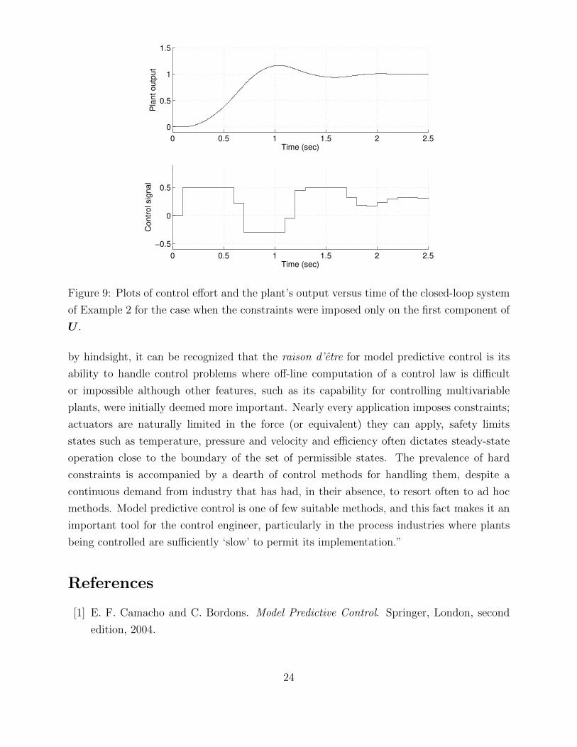
Example 2 In this example, we apply the discrete MPC controller from Example 1 to the

continuous plant modeled by (38). The MPC controller’s objective is to force the plant’s

output to track the unit step. The zero-order hold is applied to the discrete MPC controller’s

output sequence resulting in a piece-wise constant input to the continuous plant model. In

Figure 9, we show plots of the plant output as well as the control effort versus time. As in

the previous example, the prediction horizon is Np = 3 and the constraints on the control

are

−0.3 ≤ u(k) ≤ 0.5

22

0 5 10 15 20 25−0.4

−0.2

0

0.2

0.4

0.6

sampling instancescontr

ol effort

0 5 10 15 20 250

0.5

1

1.5

sampling instances

pla

nt outp

ut

Figure 8: Plots of control effort and the plant’s output versus time of the closed-loop system

of Example 1 for the case when the constraints were imposed on all the components of U .

11 Observer-Based MPC

If the plant state is not accessible, we need to use an observer in the controller implementation

as shown in Figure 10.

12 Notes

The key reason for huge popularity of the MPC approach is its ability to systematically

take into account constraints thus allowing processes to operate at the limits of achievable

performance [3]. For some impressive industrial applications of MPCs see [3, 1]. Nonlinear

model predictive controllers are presented in [6, 8]. For a comprehensive treatment of the

MPC, we recommend Maciejowski [5].

An insightful description of model predictive control is offered by Mayne et al. [7, pp. 789–

790], where they write, “Model predictive control (MPC) or receding horizon control (RHC)

is a form of control in which the current control action is obtained by solving on-line, at

each sampling instant, a finite horizon open-loop optimal control problem, using the current

state of the plant as the initial state; the optimization yields an optimal control sequence

and the first control in this sequence is applied to the plant. This is its main difference

from conventional control which uses a pre-computed control law. With the clarity gained

23

0 0.5 1 1.5 2 2.5

0

0.5

1

1.5

Time (sec)P

lan

t o

utp

ut

0 0.5 1 1.5 2 2.5

−0.5

0

0.5

Time (sec)

Co

ntr

ol sig

na

l

Figure 9: Plots of control effort and the plant’s output versus time of the closed-loop system

of Example 2 for the case when the constraints were imposed only on the first component of

U .

by hindsight, it can be recognized that the raison d’etre for model predictive control is its

ability to handle control problems where off-line computation of a control law is difficult

or impossible although other features, such as its capability for controlling multivariable

plants, were initially deemed more important. Nearly every application imposes constraints;

actuators are naturally limited in the force (or equivalent) they can apply, safety limits

states such as temperature, pressure and velocity and efficiency often dictates steady-state

operation close to the boundary of the set of permissible states. The prevalence of hard

constraints is accompanied by a dearth of control methods for handling them, despite a

continuous demand from industry that has had, in their absence, to resort often to ad hoc

methods. Model predictive control is one of few suitable methods, and this fact makes it an

important tool for the control engineer, particularly in the process industries where plants

being controlled are sufficiently ‘slow’ to permit its implementation.”

References

[1] E. F. Camacho and C. Bordons. Model Predictive Control. Springer, London, second

edition, 2004.

24

Observer-based MPC

cost function

u(ti) y(ti)+_

predictederror

predictedoutput

PlantModel

Optimizerpredicted

input Plantr( ).

x(ti) Observer

constraints

Figure 10: MPC implementation when the plant’s state is not available.

[2] E. K. P. Chong and S. H. Zak. An Introduction to Optimization. John Wiley & Sons,

Inc., Hoboken, New Jersey, fourth edition, 2013.

[3] B. Kouvaritakis and M. Cannon, editors. Nonlinear Predictive Control: Theory and

Practice. The Institution of Electrical Engineers, London, 2001.

[4] D. G. Luenberger. Linear and Nonlinear Programming. Addison-Wesley Publishing,

Reading, Massachusetts, second edition, 1984.

[5] J. M. Maciejowski. Predictive Control with Constraints. Prentice Hall, Harlow, England,

2002.

[6] D. Q. Mayne and H. Michalska. Receding horizon control of nonlinear systems. IEEE

Transactions on Automatic Control, 35(7):814–824, July 1990.

[7] D. Q. Mayne, J. B. Rawlings, C. V. Rao, and P. O. M. Scokaert. Constrained model

predictive control: Stability and optimality. Automatica, 36(6):789–814, June 2000.

[8] H. Michalska and D. Q. Mayne. Moving horizon observers and observer-based control.

IEEE Transactions on Automatic Control, 40(6):995–1006, June 1995.

[9] S. G. Nash and A. Sofer. Linear and Nonlinear Programming. McGraw-Hill, New York,

1996.

[10] A. L. Peressini, F. E. Sullivan, and J. J. Uhl, Jr. The Mathematics of Nonlinear Pro-

gramming. Springer-Verlag, New York, 1988.

[11] L. Wang. Model Predictive Control System Design and Implementation Using MATLAB.

Springer, London, 2009.

25