an introduction to numerical analysis 1 introduction this manuscript provides an introduction to...
TRANSCRIPT
An Introduction to Numerical Analysis
James Brannick
The Pennsylvania State University


Contents
Chapter 1. Introduction 5
Chapter 2. Computer arithmetic and Error Analysis 7
Chapter 3. Approximation and Interpolation 17
Chapter 4. Solutions of Linear Systems 25
Chapter 5. Numerical solution of non-linear equations 49
3


CHAPTER 1
Introduction
This manuscript provides an introduction to Numerical Analysis, covering themost basic numerical methods and their implementation. Numerical methods areused for many applications of computers and computing in practice. They cer-tainly play an important role in modern Biology, Chemistry, Engineering, Finance,Physics, and in other areas. A good numerical method typically yields more accu-rate results and is much faster than a poorly designed approach. In fact, improvingthe speed of the algorithms is as important as improving the speed of hardware,and the improvements in the speed of the algorithms have kept pace with the im-provements in the speed of hardware over the last decades. More recently, theimprovements in the speed of algorithms have even outpaced improvements in thespeed of hardware. Moreover, as computer architectures evolve, the required prop-erties of an algorithm to run efficiently when it is implemented also change. Thismanuscript is intended to serve as an introduction to the design, mathematicaltheory and implementation of algorithms for numerical methods.
5


CHAPTER 2
Computer arithmetic and Error Analysis
This chapter focuses on the computer representation of numbers in the binarynumber system and the details of finite precision binary numbers and round-offerror. These issues in turn can lead to errors in computation when algorithmsare implemented and then used to solve practical problems with computers. Italso covers some typical mistakes that can result in large errors, leading to loss ofsignificance in the computed results.
The main focus of this chapter is on understanding how a computer handlesbasic arithmetic calculations, independent of the algorithms (or numerical meth-ods) that motivate these calculations. For instance, computer arithmetic leads toround-off errors, which do not arise when infinite precision is used (as in abstractmathematical calculations).
Specifically, this chapter covers the following topics:
• The decimal and binary systems and their relation.
• Normalized scientific notation.
• Machine numbers.
1. Decimal versus binary systems: Integers.
It is useful to consider the representation of integers and that of general realnumbers separately, since these are treated differently in the computer. Integers(such as 1, 0,−1, 2013, . . .) can be represented exactly both in real life and by com-puters in a given number system. Generally, a number system with base b, for aninteger b ≥ 2, has b digits. For instance, if b = 2, the set of digits is {0, 1}. If thebasis b = 10, then the number system will have 10 digits, {0, 1, ..., 9}. However, ifthe basis is 16 (hexadecimal system, sometimes used by computers to print results),then additional digits are needed:
{0, 1, . . . , 9, A,B,C,D,E, F}
Given a basis b, the resulting number system is defined as follows.
eq:basisrep Definition 2.1. Let b0, b1, . . . , bn be digits in basis b. Then
(bnbn−1bn−2 . . . b1b0)b = bnbn−1bn−2 . . . b1b0(b) := b0 + b1b+ . . .+ bnbn.
Examples: Conversion from binary to decimal F = 1111(2) = 1+2+4+8 =15, 10101(2) = 1 + 4 + 16 = 21.
An example of a C++ code that implements the conversion from binary todecimal is given below C++ code for computing p = bnb
n+bn−1bn−1 + . . .+b0.
Assume that the coefficients bk, the integer n, and the value b are given.
7

8 2. COMPUTER ARITHMETIC AND ERROR ANALYSIS
int k ;p = .0;for(k = n; k >= 0; −− k) p = p*b + b[k];
To convert from binary to decimal, we set b = 2.
The algorithm described above is called Horner’s scheme. This algorithm isvery useful for computing values of polynomials. More details on this are given ina following chapter on polynomial interpolation.
Similarly, for real numbers let
bn, bn−1, . . . , b1, b0, b−1, . . .
be digits in basis b. Then
eq.representeq.represent (1) ± (bnbn−1bn−2 . . . b1b0.b−1b−2 . . . b−k . . .)(b)
:= ±(bnbn + bn−1b
n−1 + . . .+ b1b+ b0 + b−1b−1 + . . . b−kb
−k + . . .)
= ±n∑
k=−∞
bkbk
Note that every real number can be represented in the form above. The sum isactually a series, so the infinite sum is a limit. The series consists of positivenumbers and can be shown to be convergent since b−kb
−k ≤ (b− 1)b−k and
eq.series.beq.series.b (2)
∞∑k=1
(b− 1)b−k = (b− 1)b−1
1− b−1= 1.
Examples:.011(2) = 1/4 + 1/8 = 3/8.
Equation (eq.series.b2) shows that for b = 2 and b− 1 = 1
(0.11111 . . .)(2) = 1(2)
This means that the writing of a number in a basis may not be unique. The samephenomenon is encountered in basis 10 (decimal system)
0.99999 . . . = 1.
Only the numbers of the form N/10k can be represented exactly in basis 10,where N denotes a general integer. Similarly, only the numbers of the form N/2k
can be represented exactly in basis 2, where N again denotes an arbitrary inte-ger. Signicantly fewer real numbers can be represented exactly in a computer, asdiscussed in subsequent sections of the chapter.
Examples: Conversion from decimal to binary To convert an integer N tobinary, the number N is divided by 2 with remainder until the result is zero, wherethe remainders give in order the digits b0, b1, . . . , bn.For instance, to convert 23 to binary, we can perform the following steps:

2. DECIMAL VERSUS BINARY SYSTEMS: REAL NUMBERS. 9
23/2 = 1112 , remainder b0 = 1.
11/2 = 512 , remainder b1 = 1.
5/2 = 212 , remainder b2 = 1.
2/2 = 1, remainder b3 = 0.1/2 = 1
2 , remainder b4 = 1.
Hence 23 = 10111(2).
Similarly, −57 = −111001(2), 117 = 1110101(2), 1097 = 10001001001(2), −389 =−110000101(2). A computer program that implements this procure is as follows.Let m be the given number that has to be converted and n its maximum allowednumber of digits. The variable q is an auxiliary variable used to divide by 2 withremainder. Assume for simplicity that m ≥ 0, note however that the program“binaryInt.cpp” deals also with the case of negative numbers, with the sign beingsaved as the last entry in the array (bn, bn−1, ..., b0).
Pseudocode for “binaryInt.cpp”
input n;do the following for k from 0 to n− 1, increasing each time k by 1:{
q ← m/2;compute the remainder: bk ← m− 2 ∗ q;if q = 0, break (stop) the cycle;m← q;
}
Resulting C++ piece of code:
int k, m, n, q;for(k = 0; k < n; + + k){
q = m/2;b[k] = m− 2 ∗ q;if(q == 0) break;m = q;
}
Note that the code will run even if the break command is omitted, but this willlead to a few unnecessary operations.
2. Decimal versus binary systems: Real numbers.
Recall that
eq.representeq.represent (3) ± (bnbn−1bn−2 . . . b1b0.b−1b−2 . . . b−k . . .)(b)
:= ±(bnbn + bn−1b
n−1 + . . .+ b1b+ b0 + b−1b−1 + . . . b−kb
−k + . . .)
= ±n∑
k=−∞
bkbk

10 2. COMPUTER ARITHMETIC AND ERROR ANALYSIS
For instance, 10.011(2) = 2 + 1/4 + 1/8 = 19/8.
Let a repeated group of digits z in the decimal part be denoted (z). Then
(0.11111 . . .)(2) = 0.(1)(2) = 1,
(0.00101010101 . . .)(2) = 0.0(01)(2),
Sox = (0.1010101 . . .)(2) = 0.(10)(2).
Thus 4x = 4(0.1010101 . . .)(2) = (10.1010101 . . .)(2) = 10(2) + x = 2 + x. This gives3x = 2, and hence x = 2/3.
Similarly let
y = (11.010010010010 . . .)(2) = 11.(010)(2) = 3 + .(010)(2) = 3 + x.
wherex = .(010)(2).
Then 8x = 8(0.010010010010010 . . .)(2) = (10.010010010010010 . . .)(2) = 10(2)+x =2 + x. This gives 7x = 2, and hence x = 2/7.
3. Conversion to binary of real decimal numbers
Denote by [x] the integer part of x. Thus [x] is the unique integer satisfying
[x] ≤ x < [x] + 1.
For example, [3.14152] = 3, [−1.0001] = −2.The sign is preserved (that is, it does not change in conversion), so only the
conversion of a positive real number x to binary is presented. Since conversion ofan integer to binary was covered already, this section focuses only on conversionof the fraction part of a real number. Let x = [x] + y, with 0 ≤ y < 1 considerconverting y to binary. Changing the indexing and assuming the convention thatthe digits in the fractional part are ordering in ascending order let
y = (0.b1b2 . . . bk . . .)(2)
The following conversion procedure is based on the observation that 2y = (b1.b2 . . . bk . . .)(2),and hence b1 = [2y] and (0.b2 . . . bk . . .)(2) = 2y − [2y]. The next digit b2 is com-puted in the same way, but with y replaced by 2y − [2y]. As an example, considerconverting y = 3/7 to binary using this procedure:
b1 = [2y] = [6/7] = 0, 2y − [2y] = 6/7− 0 = 6/7,b2 = [2 6
7 ] = [12/7] = 1, 12/7− [12/7] = 5/7,
b3 = [2 57 ] = [10/7] = 1, 10/7− [10/7] = 3/7,
b4 = [2 37 ] = 0, 6/7− 0 = 6/7.
Now, the calculation for b4 is the same as the one for b1, and hence the calculationsrepeat. That means b5 = b2, b6 = b3, and so on. Thus,
3/7 = (0.011011011011 . . .)(2) = 0.(011)(2) .
Similarly1/5 = (0.0011001100110011 . . .)(2) = 0.(0011)(2) .
and1/3 = (0.01010101 . . .)(2) = 0.(01)(2) .

4. MACHINE INTEGERS 11
The conversion algorithm described above (for real numbers from decimal to bi-nary) has the following implementation. Given a number x, its binary digits will bestored in the vector (array) (b1, b2, ..., bn) of length n, the number of computed digitsfor y after the radix point, assuming that 0 ≤ y < 1, so that y = (0.b1b2 . . . bn . . .)(2).
Pseudocode for binaryReal.cpp
input y;do the following for k from 1 to n, increasing each time k by 1:{
bk ← [2y];y ← 2y − bk;
}
Resulting C++ piece of code:
int k, b[MAX];for(k = 1; k <= n; + + k){
b[k] = (int) (2.*y);y = 2*y - b[k];
}
Note: the operator “(int)” is not necessary, since b[k] is an integer variable, sothe result of 2.*y will be saved as an integer anyway.
Review example: Convert −11/7 to binary: −1.(100)(2) and then check yourresult using the program binaryReal.cpp.
4. Machine integers
Typically integers are stored in single precision using 4 bytes of memory, whichrepresents 32 bits. One bit is reserved for the sign. That leaves 31 bits for thepositive part. The largest integer that can be represented using 31 bits is Nmax =231 − 1 = 2, 147, 483, 647 (about 2 billion). So the computer can only representintegers between −Nmax and Nmax (using four bytes). This means that one cancount on 9 exact digits of accuracy for an integer.
In particular, the evaluation using a computer of arithmetic expressions that wouldnormally lead to results outside this range will result in wrong results (referred toas overflow).
Example: Test examples of overflow in Matlab by adding large numbers.

12 2. COMPUTER ARITHMETIC AND ERROR ANALYSIS
5. (Computer) normalized scientific notation
For simplicity, only the case of the binary system will be considered. Let x bea non-zero number represented in binary. Then we can write x as
eq.sci.noteq.sci.not (4) x = ±(bnbn−1bn−2 . . . b1b0.b−1b−2 . . . b−k . . .)(2)
= ±(1.bn−1bn−2 . . . b1b0.b−1b−2 . . . b−k . . .)(2) × 2n
where we have assumed that bn = 1, since otherwise we could just drop this digitas insignificant.
The (computer) normalized scientific notation is then
x = ±(1.f)(2) × 2e
where f is called the mantissa and the integer e is called the exponent. Notethat there is always exactly one “1” to the left of the radix point. This “1” is the“implicit bit,” and is not represented in the computer. (To be more precise, it willsometimes be 0, that is the case for the so called “subnormal machine numbers,”see below.)
Example: −(.00101)(2) = −(1.01)(2) × 2−3 and 10110(2) = 1.0110× 24.
In single precision (4 bytes), the sign occupies one bit, the exponent occupies8 bits (7 for the digits and one for the sign) and mantissa (excluding the implicit“1” in 1.f for normal machine numbers, respectively “0” in 0.f for submnormalmachine numbers) occupies the remaining 23 bits.
The exponent e must satisfy −126 ≤ e ≤ 127, and the computer stores m =e + 127, a positive number called biased exponent. Since 1 ≤ m ≤ 254 = 28 − 2,that leaves two more possibilities for m: m = 0 and m = 255, which have a specialsignificance. Without entering into too much details, the case m = 0 is used forinstance to represent the number 0, which in fact has two representations +0 and−0, and m = 255 is used to represent, for instance, ∞ or NaN (not a number).
6. Floating point machine numbers
The number εm := 2−23 plays a special role and is called machine epsilon. Itis the smallest positive number such that 1 + ε is a machine number 6= 1. Notehowever that 2 + εm will be represented as 2 (in single precision, more about thisin the next section).
The smallest positive normal machine number is 2−126 (e = −126, m = 1, andf = 0). The largest normal machine number is 2127(2 − εm) (e = 127, m = 254,f = (111 . . . 11)(2), with 23 digits of 1).
The numbers represented using 0 < m < 255 are called normal single-precisionmachine numbers. The numbers represented using m = 0 are called subnormalsingle-precision machine numbers. For subnormal machine numbers the implicitbit is assumed to be actually 0. Note, however, that in this case, the exponent ise = −126, and not m− 127 = −127. This is to avoid creating some artificial gaps

7. IEEE ROUNDING APPROXIMATION 13
in the numbers that are represented, since instead of the 1 in 1.f , this can alsobe defined by making the implicit bit to be 0. Together, the normal and subnor-mal (single precision) machine numbers form the set of single-precision machinenumbers. These are the only numbers that we can represent exactly in acomputer using single precision. (The single precision variables are declaredusing “float” in C++.) If x is machine number (normal/subnormal), then −x isalso a machine number (normal/subnormal).
The subnormal single-precision machine numbers have absolute values smallerthan the absolute values of the normal single-precision machine numbers. Theconstant 0 is an example of a subnormal number. This is because for subnormalnumbers e = m − 127 = −127 and the implicit bit is assumed to be zero, not 1as for normal numbers. Thus the largest (positive) subnormal machine number is2−126(1− εm) = 2−126(1− 2−23) just slightly less than 2−126, the smallest positivenormal (single precision) machine number. On the other hand, the smallest positive(single precision) submnormal machine number is 2−126εm = 2−149.
Since εm is approximately 1.2× 2−7, typically single precision gives about sixexact digits of accuracy. By contrast, in double precision, εm = 2−52 ≈ 2.2×10⁻¹⁶,giving about 15 exact digits. This is because in double precision, 8 bytes (=64bits) of memory are used to store the number. Of these, 11 bits are allocated tothe (biased) exponent m = e + 1023, which for normal double precision machinenumbers must satisfy again 1 ≤ m ≤ 2046. The case m = 0 is reserved forsubnormal (double precision) machine numbers, for which the implicit bit is 0, not1 as for normal (double precision) machine numbers.
7. IEEE rounding approximation
Let x = ±(1.f)(2)×2e, written in (computer) normalized form. Assume −126 ≤m ≤ 127 (the range for normal numbers). Only 23 digits of f can be stored. Write
1.f = 1.b1b2 . . .
where the finite writing is chosen, if one exists.
Here are some possibilities to store (part of) f in the computer:
Chopping (or truncation): In this convention, the first 23 digits of f are storedand the rest ignored.
Rounding Here, f1 is chosen such that it has 23 digits and is such that 1.f1 is theclosest to 1.f . When two such number exist (that is when b24 = 1 but bk = 0 fork > 24), we choose the largest of the two possible choices for the closest f1. Wehave therefore that rounding is the same as truncation if b24 = 0. When b24 = 1,rounding means to truncate 1.f to 1.f2, but then add 2−23 to the resulting 1.f2 toobtain 1.f1.
IEEE Rounding This is similar to rounding, except that when two choices for f1exist (that is when b24 = 1 but bk = 0 for k > 24), the f1 that ends with 0 is chosen(from among the two possible choices for the closest f1). The resulting number±(1.f1)× 2m is the machine approximation of x and will be denoted fl(x).

14 2. COMPUTER ARITHMETIC AND ERROR ANALYSIS
Examples 2.2. : Represent 1/3 as machine number. Recall that
1/3 = .(01)(2) = .0101010101...(2) = 1.01010101...(2) × 2−2.
Therefore e = −2 and f1 = 0101 . . . 01011 (23 digits). Note the last “1” whichis does not follow the periodicity rule, and which was obtained by “rounding up.”Thus
fl(1/3) = 1.01010101 . . . 01011(2) × 2−2, 23 digits after radix.
Represent 1/5 as machine number. Recall that
1/5 = .(0011)(2) = .0011001100110011 . . .(2) = 1.100110011001 . . .(2) × 2−3.
Therefore e = −3 and f1 = 1001 1001 1001 . . . 1001 101 (23 digits), where spacewas used to separate the periods. Note the last “1” which is does not follow theperiodicity rule, and which was obtained again by “rounding up.” Thus
fl(1/5) = 1.1001100110011 . . . 1001011(2) × 2−3, 23 digits after radix.
Represent −11/7 as machine number. Recall that
−11/7 = −1.(100)(2) = −1.1001001001001001...(2) × 20.
Therefore e = 0 and f1 = 100 100 100 . . . 100 10 (23 digits), where space was usedto separate the periods. This time rounding down, or truncation (or chopping) wasused. Thus
fl(−11/7) = −1.1001001001 . . . 10010(2) × 20, 23 digits after radix.
Example: Show that 2 and εm are machine numbers. Show that 2 + εm isnot a machine number. Find fl(2 + εm). The machine arithmetic is defined byx⊕ y = fl(x+ y). Find (2⊕ εm)⊕ εm and 2⊕ (εm)⊕ εm). Conclude that ⊕ is notassociative, and thus that rounding errors occur.
It turns out that the normal single precision machine numbers are the numbersof the form x = ±N/2e−23, where −126 ≤ e ≤ 127 and N is an integer 223 ≤ N ≤224 − 1. The smallest power of two that can be represented as a normal, singleprecision machine number is thus 2−126 and the largest such power is 2127. Near anumber of the form 2e, −126 < e ≤ 127, which is thus a normal, single precisionmachine number, the set of single-precision machine numbers looks as follows:
. . . , 2e(1− 3εm/2), 2e(1− εm), 2e(1− εm/2), 2e,
2e(1− εm), 2e(1− 2εm), 2e(1− 3εm), . . .
These numbers are thus more dense to the left of 2e than to the right of 2e.
A consequence of this is that each of the intervals [2e, 2e+1] with −126 ≤ e ≤126 has end points consisting of normal, single-precision machine numbers, andthe (single-precision) machine numbers in this interval divide it into 223 smallerintervals of equal size. For x ∈ [2e, 2e+1], fl(x) is the closest (single-precision)machine number. If two such numbers exist, the one whose mantissa has the lastdigit equal to 0 is chosen.

8. ROUNDING ERRORS 15
Errors: The relative error is
|x− fl(x)||x|
=|(1.f)(2) − (1.f1)(2)|2e
(1.f)(2)2e=|(1.f)(2) − (1.f1)(2)|
(1.f)(2)< εm/2,
which is pretty small (but no better estimate exists).
However, the resulting absolute error is
|x− fl(x)| = |x− fl(x)||x|
|x| < εm|x|/2,
and this is again the best possible estimate. This means that the size of the expectedabsolute error is proportional to |x|, and, in particular, it may be large if |x| is verylarge.
Consider all the negative powers of 2 that are machine numbers. Then, thereare powers of 2 that are not (single-precision) normal numbers. These powers of2 are subnormal (single-precision) machine numbers, which are numbers y of theform y = ±N2−126−23, with N an integer 0 ≤ N ≤ 223 − 1, and hence |y| < 2−126,where 2−126 is the smallest positive normal (single-precision) machine number. Inthis case, the implicit bit is 0! The smallest positive subnormal (single-precision)machine number is then 2−126−23.
8. Rounding errors
Since only machine numbers can be represented exactly in the computer, therewill necessarily be errors, since most of the time, the result of calculations will notyield a machine number. Errors can arise due to
• Input or output.• Arithmetic operators (result too big: overflow; result too small: under-
flow).
Examples:
1. Both 4 and εm := 2−23 are (single precision) machine numbers, but theirsum is not. The sum 4 + 2−23 will be rounded by the computer and stored asfl(4 + 2−23) = 4. In fact, if x = (1.f)(2) × 2−23, fl(4 + x) = 4, so there is a lossof significance: the digits of x have no significance. Thus, if x is the result of acalculation, there is no reason to try hard to improve that calculation. The sum4 + x will always be stored as 4 by the computer (if the exponent of x is −23).A situation that one wants to avoid, is thus the addition of two numbers of verydifferent magnitudes.
2. The example above can be modified to conclude that the computer will obtaindifferent results if evaluating (2+εm)+εm and 2+(εm+εm). Check this calculation!This means that if you need to add up many numbers of different magnitudes, it isbetter to start adding up the smaller numbers (in absolute value) and then continuein increasing order of magnitudes (of the absolute values). Another example isprovided by extending the above example to x0 = 2, xk = εm, k = 1, 223. Addingone by one in increasing order will give 2! However, adding first the small numberswill give 3.

16 2. COMPUTER ARITHMETIC AND ERROR ANALYSIS
3. A similar situation arises when one subtracts nearly equal numbers. Indeed, con-
sider the calculation x =√1+y−1y , where y is a (single-precision) machine number
≤ εm/2. Then the floating point approximation fl(1 + y) of 1 + y is fl(1 + y) = 1.This means that the numerator is zero, and hence, the computer will evaluate x as
0. On the other hand, we can write√1+y−1y = 1+y−1
y(√1+y+y)
= 1√1+y+y
. The later is
evaluated by the computer as being 1/2, which is actually very close to the trueresult.
4. Again, a similar problem arises when one computes ex for x << 0 using theseries ex =
∑∞k=0 x
k/k!.
The fact that real numbers can not be represented in computers leads us to thenotions of well-posed and ill-posed computation (these are sometimes called stable,respectively unstable computations, or yet well conditioned, respectively ill condi-tioned calculations). Let F (x1, . . . , xn) be an algorithm (or computation) providingas result a number in a given format (e.g. single-precision). Assume that this al-gorithm will always work (no undefined operations like division by zero) and theresult is always the same for the same data x1, . . . , xn. Then F is a well-posedcomputation if it provides always a solution and a small change in x1, . . . , xn leadto a small change in F .
Assume n = 1. Often this small change in F is guaranteed by the existence ofa constant C > 0 that is not too large such that
|F (x)− F (y)| ≤ C|x− y|,which means that F is Lipschitz with constant C. When n > 1, norms are needed.
Example 2.3. Most of the algorithms that you will encounter will be well-conditioned. However here is one that shows ill-conditioning. Let us define a0 = 1,a1 = −1 + x, and an+2 = 5an+1 + 6an. Write a program compouting a10. Run itfor x = 0 and for x very small but different from 0. Conclude that this algorithmis ill-conditioned.

CHAPTER 3
Approximation and Interpolation
1. Polynomial approximation
1.1. Statement of the problem and the main result. Let us assume thatwe are given some real numbers (points or nodes) x0 < x1 < . . . < xn and somevalues y0, y1, . . . , yn. The x and y values will be called interpolation data.
The polynomial interpolation problem is to find a polynomial P (usually ofleast degree or with some other properties) such that P (xi) = yi. A polynomial withthis property will be called a polynomial interpolating the data x0 < x1 < . . . < xnand y0, y1, . . . , yn or, simply, an interpolating polynomial.
One of the main theoretical results of this section is the solution of this problem.
thm.gen.IP Theorem 3.1. There exists a unique polynomial P0 of degree ≤ n interpolatingthe data x0 < x1 < . . . < xn and y0, y1, . . . , yn. If P is any other interpolatingpolynomial, then there exista a polynomial Q such that
eq.gen.IPeq.gen.IP (5) P (x) = P0(x) +Q(x)(x− x0)(x− x1) . . . (x− xn),
and, conversely, any polynomial of this form is an interpolating polynomial.
We shall refer to the polynomial of Equation (eq.gen.IP5) as the general interpolating
polynomial of the given data. On the other hand, we shall refer to P0 as the minimaldegree interpolating polynomial.
If we write the Interpolation Problem as a system with P =∑mi=0 aix
i, withm = deg(P ), then we see that we have m + 1 unknowns with n + 1 equations, sowe will set m = n.
The matrix of the resulting system is a Vandermoned matrix, which is non-singular, so the system can be solved. This proves the existence and uniqueness ofthe polynomial P0 in Theorem
thm.gen.IP3.1. From a practical point of view, however, this
is the wrong way to solve the interpolation problem (both as far as the proof isconcerned and as far as the construction of P0 is concerned). We will give anotherproof of the Theorem
thm.gen.IP3.1 using the Lagrange interpolating polynomial in the next
subsection.
1.2. The Lagrange interpolating polynomial and proof. Let us considerthe interpolation data x0 < x1 < . . . < xn and y0, y1, . . . , yn. We introduce the
17

18 3. APPROXIMATION AND INTERPOLATION
polynomials
eq.def.lieq.def.li (6)
Π(x) = (x− x0)(x− x1) . . . (x− xn),
`i(x) = Π(x)/(x− xi),
P0(x) =
n∑i=0
yi`i(xi)
`i(x).
The polynomials introduced in the equation right above are obtained from theconditions that Π(xi) = 0 and `i(xj) = `i(xi)δij for all i and j. The polynomials`i/`i(xi) are called Cardinal functions. It then follows that P0 is an interpolatingpolynomial for our data. Clearly P0 has degree at most ≤ n, since `i has degreeat most n. If follows that P0 is a minimum degree interpolating polynomial (westill have to prove the theorem justifying this name). The form for P0 providedby Equation (
eq.def.li6) is called the Lagrange form of the minimum degree interpolating
polynomial.
We now turn to the proof of Theoremthm.gen.IP3.1 shall need the following lemma, which
is well known (Bezout’s Lemma).
lemma.Bezout Lemma 3.2. Let T be a polynomial satisfying T (xi) = 0, i = 0, 1, . . . , n. ThenΠ|T , that is, there exists a polynomial Q such that T = QΠ.
We are now ready to prove Theoremthm.gen.IP3.1.
Proof. We have constructed a polynomial P0 satisfying the conditions of The-orem
thm.gen.IP3.1 (that is, it interpolates the data and has degree ≤ n). Let then P be any
other interpolating polynomial. Then P (xi) = yi = P0(xi) for all 0 ≤ i ≤ n. It fol-lows that the polynomial T (x) = P (x)−P0(x) satisfies T (xi) = 0 for all 0 ≤ i ≤ n,and hence T = QΠ, by Lemma
lemma.Bezout3.2. This proves the general form (
eq.gen.PI??) for the
interpolating polynomial P .Let us now complete the proof by proving the uniqueness of the polynomial
P0. Let us consider an arbitrary interpolating polynomial P of degree ≤ n. Thenwriting P −P0 = QΠ, we have that QΠ has degree ≤ n. Since Π has degree n+ 1,this is possible only if Q = 0, and hence, in fact, P = P0. �
1.3. Newton’s form of the interpolating polynomial. Consider interpo-lating data x0 < x1 < . . . < xn and y0, y1, . . . , yn, as before. Let us denote byPk the minimum degree interpolating polynomial for x0 < x1 < . . . < xk andy0, y1, . . . , yk, for all possible values of k (k = 0, 1, . . . , n). Then Pk has degree ≤ k.
Since both Pk and Pk+1 interpolate the data x0 < x1 < . . . < xk and y0, y1, . . . , yk,it follows from Theorem
thm.gen.IP3.1 that
eq.iter.Pkeq.iter.Pk (7) Pk+1 = Pk + ck+1(x− x0)(x− x1) . . . (x− xk),
for some undetermined polynomial ck+1. Counting degrees, we see that ck+1 mustbe a polynomial of degree ≤ 0, and hence ck+1 is actually a constant. Note that P0

1. POLYNOMIAL APPROXIMATION 19
is also a constant: P0(x) = y0 = c0. Iterating Equation (eq.iter.Pk7), we obtain
eq.Newton.ckeq.Newton.ck (8) Pn = Pn−1 + cn(x− x0)(x− x1) . . . (x− xn−1)
= Pn−2 + cn−1(x− x0) . . . (x− xn−2) + cn(x− x0) . . . (x− xn−1)
= P0 + c1(x− x0) + c2(x− x0)(x− x1) + . . . + cn−1(x− x0) . . . (x− xn−2)
+ cn(x− x0) . . . (x− xn−1) =
n∑k=0
ck(x− x0)(x− x1) . . . (x− xk−1).
Newton’s form of the interpolating polynomial is obtained from the above formulaby identifying the coefficients ck with suitable divided differences. Note that ck isthe coefficient of the highest power (that is, of xk) of Pk.
Definition 3.3. Assume that f(xi) = yi for some function f . We then definef [xi] = f(xi) and
f [xi, xi+1, . . . , xj ] :=f [xi+1, xi+1, . . . , xj ]− f [xi, xi+1, . . . , xj−1]
xj − xi,
which are defined whenever the points x0, x1, . . . , xn are distinct (not necessarilyincreasing).
The coefficients ck in Newton’s form of the interpolating polynomial are iden-tified by
thm.eq.coeff.Newton Theorem 3.4. We have ck = f [x0, x1, . . . , xk].
To prove the above theorem, we shall need the following lemma
lemma.ckn Lemma 3.5. Let us denote by Qn−1 the minimum degree polynomial interpo-lating our data at x1, x2, . . . , xn. Then
(Pn(x)− Pn−1(x))(xn − x0) = (x− x0)(Qn−1(x)− Pn−1(x))
Proof. Let the left hand side polynomial be denoted by L and the right handside polynomial be denoted by R. We compute using the interpolation propertyand see that L(xi) = R(xi). Since both polynomials have degree at most n, weobtain that L = R. �
We are now ready to prove Theoremthm.eq.coeff.Newton3.4.
Proof. We prove Theoremthm.eq.coeff.Newton3.4 by induction on the number n of points. Indeed,
for n = 0, c0 = f(x0) = f [x0] by definition. Assume now the statement has beenproved for all values < n. Let us compute the coefficients of the highest powers ofthe polynomials appearing in Lemma
lemma.ckn3.5. By definition, the coefficient of xn in the
left hand side polynomial is cn(xn − x0). On the other hand the coefficient of xn
in the right hand side polynomial is the difference of the cn−1 coefficients for Qn−1and Pn−1, that is
f [x1, x2, . . . , xn]− f [x0, x1, . . . , xn−1].
By Lemmalemma.ckn3.5, these two coefficients are the same, which completes the proof. �

20 3. APPROXIMATION AND INTERPOLATION
Example, compute the divided differences, the Newton form of the interpola-tiong polynomials and the Lagrange form for the interpolating polynomial.
Here are some examples:
x 0 1 2 3y 1 0 1 4−1 1 31 10
The resulting polynomial is
PN (x) = 0(x− 0)(x− 1)(x− 2) + 1(x− 0)(x− 1)− 1(x− 0) + 1
= x2 − x− x− 1 = (x− 1)2
(Exercise: compute the Lagrange form of the minimum degree interpolating poly-nomial).
x −1 0 2 3y −8 −1 1 8
7 1 7−2 21
The resulting polynomial is
PN (x) = 1(x+ 1)(x− 0)(x− 2) + (−2)(x+ 1)(x− 0) + 7(x+ 1)− 8
= x3 − x2 − 2x− 2x2 − 2x+ 7x+ 7− 8 = (x− 1)3
(Exercise: compute the Lagrange form of the minimum degree interpolating poly-nomial).
2. Error estimates
2.1. A consequence of Rolle’s Lemma. Let us assume that yi = f(xi).Then we say that P interpolates f at the nodes x0 < x1 < . . . < xn. We now wantto estimate the error that we make when we replace a function f with the minimumdegree interpolating polynomial of f at the nodes x0 < x1 < . . . < xn. We alwaysassume that f has as many derivatives as are needed to in the statements of thetheorems. Our main result is Theorem
thm.interp.error3.7 below. To prove that theorem, we need
Rolle’s Lemma and a generalization, which we combine in the following statement.
lemma.Rolle Lemma 3.6 (Rolle). Let f be an function that is n times differentiable on aninterval (a, b) and continuous on [a, b]. Assume xi ∈ [a, b] and f(x0) = f(x1) =. . . = f(xn), then
(i) there exists z1 < z2 < . . . zn, zj ∈ (xj−1, xj), such that f ′(zj) = 0, and
(ii) there exists c ∈ (x0, xn) such that f (n)(c) = 0.

2. ERROR ESTIMATES 21
Proof. The first part is Rolle’s Lemma applied to each of the intervals [xj−1, xj ].The second part follows from the first part by induction on n. �
2.2. The basic error estimate. We are now ready to formulate our mainapproximation result.
thm.interp.error Theorem 3.7. Let f be (n + 1)-times differentiable on (a, b) and continuouson [a, b]. Let xi ∈ [a, b], x0 < x1 < . . . < xn, and let P the minimum degreeinterpolating polynomial of f , that is P (xi) = f(xi) for all i. Then for any x ∈(a, b), there exists c ∈ (a, b) such that
f(x)− P (x) =f (n+1)(c)
(n+ 1)!(x− x0)(x− x1) . . . (x− xn) =
f (n+1)(c)
(n+ 1)!Π(x).
Proof. If x is one of the values xi, then there is nothing to prove; indeed,both the left and the right hand sides are equal to zero for all values of c. Letus assume then that x 6= xi for all i. Then Π(x) 6= 0 and we can define M =(n+ 1)!(f(x)− P (x))/Π(x). This gives
f(x)− P (x) =M
(n+ 1)!(x− x0)(x− x1) . . . (x− xn) =
M
(n+ 1)!Π(x).
Therefore, it is enough to show that there exists c ∈ (a, b) such that M = f (n+1)(c).To this end, let us consider the function
g(x) := f(x)− P (x)− M
(n+ 1)!Π(x).
This function has (n+ 2) roots, namely {x, x0, x1, . . . , xn}. This means that thereexists c ∈ (a, b) (this will be the c we are looking for) such that g(n+1)(c) = 0, byLemma
lemma.Rolle3.6. Therefore
g(n+1)(c) := f (n+1)(c)− P (n+1)(c)− M
(n+ 1)!Π(n+1)(c)
= f (n+1)(c)−M = 0,
because P has degree at most n and Π has degree (exactly) n + 1. We have thusproved that M = f (n+1)(c), as desired, and hence we have completed our proof. �
A similar idea can be used to prove Taylor’s formula.
Example: compute the error estimate for the interpolation error for the functionf(x) = cosx and equally spaced nodes with distance h, namely xi = ih, i =0, 1, . . . , n, and x ∈ [0, nh]. What can you say about the maximum error if nh = 1?
Solution. Let P be the minimum degree interpolating polynomial of the functionf(x) = cosx at the nodes xi = ih, i = 0, 1, . . . , n and Π(x) =
∏ni=0(x − xi), as
before. Theoremthm.interp.error3.7 gives that
f(x)− P (x) =f (n+1)(c)
(n+ 1)!(x− x0)(x− x1) . . . (x− xn) =
f (n+1)(c)
(n+ 1)!Π(x).

22 3. APPROXIMATION AND INTERPOLATION
We have that f (4k)(x) = cosx, f (4k+1)(x) = − sinx, f (4k+2)(x) = − cosx, and,finally, f (4k+3)(x) = sinx. This shows that |f (n+1(x)| ≤ 1 for all n. Therefore, theabove error estimate becomes
|f(x)− P (x)| = 1
(n+ 1)!|(x− x0)(x− x1) . . . (x− xn)| ≤ 1
(n+ 1)!max
x∈[0,nh]|Π(x)|.
It remains to estimate maxx∈[0,nh] |Π(x)|. Here is a rough estimate. We see thatthe maximum of |Π(x)| on the interval [0, nh] must be obtained in the intervals[0, h] and [(n−1)h, nh]. This shows |Π(x)| ≤ h ·h · (2h) · (3h) . . . nh ≤ n!hn+1. Thisgives |f(x)− P (x)| ≤ hn+1/(n+ 1).
In case nh = 1, we further obtain |f(x)− P (x)| ≤ 1nn(n+1) → 0 (very fast!).
2.3. Some codes. It is easy to compute the value PN (x) of the Newton in-terpolating polynomial. Let PN (x) =
∑nk=0 ck(x− x0)(x− x1) . . . (x− xk−1), with
ci and xi given as some arrays (vectors). Then to compute PN (x) for some givenx, we can use the Horner-Newton scheme that is based on writing
PN (x) =(. . .((cn(x− xn−1) + cn−1)(x− xn−2) + cn−2
). . .+ c1
)(x− x0) + c0.
This leads to the following
Resulting C++ piece of code:
// (declare and input variables first)p = c[n];for(i = n− 1; i >= 0; −−i) p = p *(x-x[i]) + c[i];
The coefficients c[i] are given by divided differences. Here is a piece of codethat gives only the divided differences needed for interpolation. We assume that fis given as a program function.
Resulting C++ piece of code:
// (declare and input variables first)for(i = 0; i <= n; ++i) c[i] = f(x[i]);for(j = 1; j <= n; ++j) {
for(i = n; i >= j; −−i)c[i] = (c[i] - c[i-1])/(x[i] - x[i-j]);
}
Exercice: Write a code that computes all the finite differences.

2. ERROR ESTIMATES 23
2.4. Chebyshev polynomials. For equally spaced nodes, the interpolationerror will tend to be exceedingly large towards the end points of the interpolationinterval. This is called the “Runge phenomenon” and is related to large oscillations(“polynomial wiggle”) of the polynomial Π(x) =
∏i(x− xi) for x close to the end
points of the interval determined by the equally spaced nodes xi.
A different choice of interpolation points (or nodes) xi often leads to betterresults. The Chebyshev polynomials Tn(x) are defined by Tn(x) = cos[n arccos(x)]and are easily seen to have n real and distinc roots in the interval (−1, 1) (exercice!).
The (n + 1)–Chebyshev interpolation points xCi on [−1, 1] are defined as thezeroes of Tn+1. The Chebyshev polynomials satisfy the recursion relation Tn+1(x) =2xTn(x)−Tn−1(x). In particular, Tn+1 has degree n+1 and the coefficient of highestdegree is 2n+1,
Tn+1(x) = 2n+1xn+1 + . . . = 2n+1(x− xC0 )(x− xC0 ) . . . (x− xC0 ).
From the definition, we also have |Tn+1(x)| ≤ 1 for x ∈ [−1, 1]. Consequently
(9)∣∣ n∏i=0
(x− xCi )∣∣ ≤ 1
2n+1, ∀x ∈ [−1, 1],
which is the least bound for any other choice of n+ 1 points in [−1, 1].
2.5. Splines. As we have seen, polynomial interpolation may yield large errrostowards the end of the interval. Sometimes a different type of interpolation maybe more useful. We now study an alternative to polynomial interpolation.
Definition 3.8. Let us consider again nodes x0 < x1 < . . . < xn. A degree kspline associated to these nodes is a function s : [x0, xn]→ R that is a polynomialof degree ≤ k on each of the intervals [xj , xj+1] and has the property that all thederivatives of order ≤ k − 1 of s are continuous functions.
For instance, a linear spline is a continuous function s that is linear on each ofthe intervals [xj , xj+1].
Let us fix the degree k of a spline s and assume that it interpolates some valuesyj . Then on each of the intervals [xj , xj+1] we must specify k + 1 parameters(the coefficients of a polynomial of degree ≤ k). This gives n(k + 1) parameters.The values of s are determined at the end points of the interval [xj , xj+1], by theassumption that s interpolates the function at these points. This gives 2n equations.The continuity requirement for s will then be automatically satified. The continuityrequirement for s′, . . . , sk−1 at each of the nodes x1, . . . , xn−1 gives k− 1 equationsfor each node. Since we have n − 1 such nodes, we obtain from the continuityrequirements a total of (n− 1)(k− 1) equations, for a total of (n− 1)(k− 1) + 2n =(n− 1)(k + 1) + 2 equations. All in all, we get
(10) n(k + 1)− (n− 1)(k + 1)− 2 = k − 1
free parameters for our spline. In particular, a linear spline s (k = 1) is completelydetermined by the values of s at the nodes.
A cubic spline s, however, will not be completely determined by the valuess(xj), but will have k − 1 = 2 free parameters. A convenient choice of theseparameters is to set s′′(x0) = s′′(xn) = 0, which leads to the concept of a natural

24 3. APPROXIMATION AND INTERPOLATION
spline. It follows that a natural spline is completely determined by the values ofs at the nodes. A common method to determine an interpolating natural cubicspline is to choose zj = s′′(xj) as the unknowns. The function s′′ is then a linearspline, and hence completely determined by the values zj . Repeated integrationthen identifies s in terms of zj and leads to a triangular system.
Here are some details. Let hi = xi+1−xi. First his′′(x) = zi(xi+1−x)+zi+1(x−
xi) by the Lagrange interpolation formula. Therefore, by taking two derivatives,we get that the function 6his(x)− zi(xi+1 − x)3 − zi+1(x− xi)3 is linear, hence
s(x) =zi
6hi(xi+1 − x)3 +
zi+1
6hi(x− xi)3 + C(x− xi) +D(xi+1 − x),
with C = yi+1/hi − zi+1hi/6 and D = yi/hi − zihi/6 determined from the valuesyi = s(xi). Writing then that the values of s′ from left and right at xi have tomatch, we obtain a tridiagonal system AZ = v, where
(11) A =
u1 h1 0h1 u2 h20 h2 u3
un−2 hn−2hn−2 un−1
where hi = xi+1 − xi, as before, and ui = 2(hi + hi−1), bi = 6(yi+1 − yi)/hi,vi = bi = bi−1.

CHAPTER 4
Solutions of Linear Systems
We have seen that Newton’s method for systems reduces to solving a non-linearsystem to solving many linear systems. Linear systems arise in many practicalapplications, so it is important to understand them well.
1. Review of linear algebra
The (explicit) general form of a linear system with n equations and m un-knowns.
1.1. Linear systems and matrices. Operations with matrices: addition,scalar multiplication, and matrix multiplication. (Stress the non-commutativity ofthe matrix multiplications, also zero divisors and nilpotent elements.)
Example: the code for the multiplication of two matrices of sizes m × n andn× q. The simplest form requires three nested loops with mnq multiplications.
A system in matrix form AX = b, with A an n ×m matrix, where m is thenumber of unknowns and n is the number of equations.
The identity matrix. Left and right inverse matrices. Example of a matrix witha left inverse, but no right inverse. The inverse matrix. Solving a linear system byinverting the system matrix.
We have the following.
thm.for.systems Theorem 4.1. Let A be an n×m matrix.
(i) The matrix A has a left inverse↔ the system AX = b has at most one solutionfor any b.
(ii) The matrix A has a right inverse ↔ the system AX = b has at least onesolution for any b.
We denote by Rn the set of n × 1 (column) matrices. Whenever needed, wewill identify a row matrix with a column matrix.
Invertible matrices can be characterized in many way, the most convenient onebeing the the determinant. To recall the definition of the determinant, we firstneed to recall the sign of a bijection. Let π : {1, 2, 3, . . . , n} → {1, 2, 3, . . . , n} bea bijection. Let us denote by I(π) the number of pairs (i, j), i < j, such thatπ(i) > π(j). The number I(π) is called the number of invertions of π. Then thesign sign(π) of π is defined by
sign(π) := (−1)I(π).
25

26 4. SOLUTIONS OF LINEAR SYSTEMS
It satisfies
sign(π1 ◦ π2) = sign(π1) sign(π2)
and sign(τ) = −1 if τ(x) = x with the exeption of two elements i < j, for whichwe have τ(i) = j and τ(j) = i (such a bijection is called a transposition).
Let A = [aij ] be now an n × n matrix. We define Sn to be the set of allpermutations of {1, 2, . . . , n} and then we define the determinant of A by
eq.def.deteq.def.det (12) det(A) :=∑π∈Sn
sign(π)a1π1a2π(2)a3π(3) . . . anπ(n).
The determinant is defined only for square matrices.
The formula (eq.def.det12) requires (n−1)n! multiplications to compute the determinant,
and hence it is prohibitively expensive to use in practice even for moderately largen.
Upper and lower triangular (square) matrices L and U .
The determinant of an upper or lower triangular matrix is the product of thediagonal elements.
We have the following characterization of invertible matrices, of which the mostuseful one is (4).
thm.prop.inverse Theorem 4.2. For an n× n matrix A, the following are equivalent:
(1) A has a left inverse.(2) A has a right inverse.(3) A has an inverse.(4) det(A) 6= 0.(5) The columns of A are linearly independent vectors in Rn.(6) The columns of A span Rn.(7) The columns of A form a basis of Rn.(8) The rows of A are linearly independent vectors in Rn.(9) The rows of A span Rn.
(10) The rows of A form a basis of Rn.(11) The linear map A : Rn → Rn (ie left multiplication by A) is injective.(12) The linear map A : Rn → Rn is surjective.(13) The linear map A : Rn → Rn is bijective.(14) AX = 0 implies X = 0.(15) AX = b has at most one solution for any b ∈ Rn.(16) AX = b has at least one solution for any b ∈ Rn(17) AX = b has exactly one solution for any b ∈ Rn.(18) A is a product of elementary matrices.(19) 0 is not an eigenvalue of A .(20) The transpose AT is invertible.
Almost all of the above statements are trivially equivalent (sometimes by defi-nition). What is non-trivial is to show that (4) is equivalent to invertibility. Thisis proved using the properties of the determinant.

1. REVIEW OF LINEAR ALGEBRA 27
In fact, here is a similar theorem about the existence of the left inverse ofa matrix A that is not necessarily a square matrix, which can be used to proveTheorem
thm.prop.inverse4.2/
thm.prop.left.inverse Theorem 4.3. For an n×m matrix A, the following are equivalent:
(1) A has a left inverse.(2) AT has a right inverse.(3) The columns of A are linearly independent vectors in Rn.(4) The rows of A span Rm.(5) The linear map A : Rm → Rn is injective.(6) The linear map AT : Rn → Rn is surjective.(7) AX = 0 implies X = 0.(8) AX = b has at most one solution for any b ∈ Rn.
If any of these properties holds true (equivalently all hold true), then n ≥ m.
Let us recall now the most important properties of the determinant.
thm.prop.det Theorem 4.4. Let A and B be two n×n matrices. Then we have the following.
(1) det(AB) = det(A) det(B).(2) det(AT ) = det(A).(3) If B is obtained from A by multiplying a row or column by λ, then det(B) =
λ det(A).(4) det(λA) = λn det(A).(5) If B is obtained from A by switching two rows or two columns, then
det(B) = −det(A).(6) If A has two identical rows or columns, then det(A) = 0.(7) If B is obtained from A by adding a multiple of a row to another row, then
det(B) = det(A). The same holds for columns.(8) We have det(A) = 0 if, and only if, a row of A is a linear combination of
the other rows. The same holds for columns.(9) Let Aij be the determinant of the matrix obtained from A by removing the
row and column containing the entry aij. Then
det(A) =n∑j=1
(−1)i+jaijAij .
(10) Let us denote by A∗ is the transpose of the matrix [(−1)+jAij ]. Then
AA∗ = A∗A = det(A)I,
where I is the identity matrix, as usual.item.inverse (11) If det(A) 6= 0, we have
A−1 = det(A)−1A∗.
ex.inv.2x2 Example 4.5. The matrix
A =
[a bc d
]has determinant det(A) = ad− bc and its inverse is
A−1 =1
ad− bc
[d −b−c a
]

28 4. SOLUTIONS OF LINEAR SYSTEMS
Exercise 4.6. Write a program that solves a 2× 2 system using the formulasof Example
ex.inv.2x24.5.
The formula (item.inverse11) of Theorem
thm.prop.inverse4.2 is not convenient for larger values of n, not
even for n = 3. For n even larger, it is prohibitively expensive to use this formulato calculate A−1, since it requires of the order of n2×n! operations to obtain A−1.Other methods will be devised to compute A−1.
Remark 4.7. When we have a simple way to find the inverse A−1 of a matrixA, then the system AX = b can be solved simply by X = A−1b. However, mostof the methods that we will learn will find the solution X without finding A−1. Infact, a simple method to find A−1 is to solve all the systems AX = ej , j = 1, . . . , n,where ej has 1 on the jth position and zero everywhere else.
1.2. Cramer’s rules. Let us consider a square, n × n system AX = b. Wedenote by ∆ the determinant of the matrix of the system and by ∆j the determinantobtained by replacing the column corresponding to xj with b. Then
eq.Cramereq.Cramer (13) xj =∆j
∆
2. Gaussian elimination
Gaussian elimination reduces the solution of a system to the solution of atriangular system. To see the advantage of that, let us look first at how to solve asystem with an upper triangular matrix.
Let us consider then the system UX = b, with U upper triangular. The solutionof this n × n system is then obtained solving first for xn, then substituting inthe equation for xn−1, and so on and so forth. Namely, xn = bn/un,n, xn−1 =(bn−1 − un−1,nxn)/un−1,n−1, . . ., with the last determined unknown given by
x1 = (b1 − u1,2x2 − u1,3x3 − . . .− u1,nxn)/u1,1
Resulting C++ piece of code:
// (declare and input variables first)for(i = n− 1; i >= 0; −− i) {
x[i] = b[i];for(j = i+ 1; j < n; + + j) x[i] = x[i] - u[i][j]*x[j];if(absVal(u[i][i]) > epsilon) x[i] = x[i]/u[i][i];else {
cout << “ ERROR MESSAGE “ << endl;break;
}}
Gaussian elimination transforms a given system AX = b into an upper tri-angular (but not necesarrily square) system by performing suitable “elementaryoperations” on the system. More precisely, one successively uses equations to elim-inate unknowns from the later equations.

2. GAUSSIAN ELIMINATION 29
In its simplest form of the Gaussian elimination, the naıve Gaussian eliminationwill use the first equation to eliminate x1 from the remaining equations. Then itwill use the second equation to eliminate x2 from the remaining equations (thethird, the fourth, and so on), and so on and so forth. In general, the coefficient ofthe unknown in the equation we use to eliminate it will be called pivot.
In the end, some of the unknowns may become parameters, so that the resultingsystem will be a true (square) upper-triangular system. This step in the Gaussianelimination method is called forward elimination.
Not every system has a solution, and Gaussian elimination (with infinite pre-cision arithmetic!) will allow us to decide whether a given system has a solution ornot. More precisely, once the reductions have been performed, the system will failto have a solution if equations of the form 0 = b′k. The resulting upper triangularsystem is then solved, if possible. This second step in the Gaussian eliminationmethod is called back substitution.
It is convenient to put together the matrix of the system A and the free termb forming the so called augmented matrix A = [Ab].
The transformation to an upper triangular system (forward elimination) isachieved by so called elementary operations:
(i) Add a multiple of an equation to another, that is, add a multiple of a row of
A to another: Ei ← Ei + λEj .(ii) Interchange two equations, that is, interchange two rows in A: Ei ↔ Ej .(iii) Multiply an equation by a non-zero number λ, that is, multiply a row of A by
λ 6= 0: Ei ← λEi.
Remark 4.8. Each of the elementary operations corresponds to the left mul-tiplication of A by an elementary matrix.
Remark 4.9. The first two kinds of elementary operations do not change thedeterminant of A (if A is a square matrix, to start with).
Two systems that are obtained from each other by elementary operations arecalled equivalent. Two equivalent systems will have the same set of solutions.
Let us assume that we apply elementary operations to the system AX = b andlet us denote by A(k) the resulting matrices after we eliminate k−1 unknowns from
the remaining equations. Thus A = A(1). Also, let us denote by A(k) = [a(k)ij ].
The method that uses only the first type of elementary operations and only
a(k)kk as pivots is called naıve Gaussian elimination. Not every system can be
solved using naıve Gaussian elimination.
Example 4.10. Solve the systemx+ 2y − 3z = 0
2x+ y = 3
x+ y + 3z = 5

30 4. SOLUTIONS OF LINEAR SYSTEMS
using naıve Gaussian elimination. (The first pivot is 1 and the solution is (1, 1, 1)).
ex.NoNGE Example 4.11. Solve the system{εx+ y = 1
x+ y = 2
using naıve Gaussian elimination for ε a very small machine number (0 < ε < εm/4,where εm is “machine epsilon”) using both infinite precision and machine precision.In infinite precision we get x = 1/(1− ε) ≈ 1 and y = (1− 2ε)/(1− ε) ≈ 1, whereasusing Gaussian elimination and machine precision, we get y = fl(2 − ε−1)/fl(1 −ε−1) = 1, which then substituting into the first equation gives x = 0, for a largerelative and absolute error!
Here is an example of a system for which the general solution is written usingparameters.
Example 4.12. Find the values of a for which the following system has at leastone solution and then solve for those values of a using naıve Gaussian elimination.
−x+ 2y + z = 5
y − z = 2
−x+ 3y = 7 + a
The solution is a = 0 and (x, y, z) = (3t− 1, t+ 2, t), with t a real parameter.
Let us denote by n the size of the matrix A to which we apply naıve Gaussianelimination to solve the system AX = b. Then the forward elimination part of thecode is as follows, where k determines the pivot akk, i is the index of the row (orequation) to be simplified, and j is the second index of the element simplified inthe row i.
C++ piece of code for Gaussian elimination:
// (declare and input variables first)for(k = 0; k < n− 1; + + k) {
if( absVal(A[k][k]) < tol) {cout << “\nWe need pivoting\n”;return 0; }
for(i = k + 1; i < n; + + i) {lambda = A[i][k]/A[k][k];for(j = k; j < n; + + j) A[i][j] = A[i][j] - lambda*A[k][j];b[i] = b[i] - lambda*b[k];
}}
Operation count: n3/3.The naıve Gaussian elimination leads to the LU factorization of A. More pre-
cisely, each time when we perform a step in the naıve Gaussian elimination, itamounts to multiply A to the left with a lower triangular matrix. Namely, at eachstep, A is replaced with LjA, where Lj is lower triangular. At the end, A is re-placed with LNLN−1 . . . L2L1A = U , with U upper triangular. Since the productof lower triangular matrices is a lower triangular matrix and the inverse of a lower

2. GAUSSIAN ELIMINATION 31
triangular matrix is also lower triangular, we obtain that A = (L)−1U = LU , whereL is lower triangular and U is upper triangular. In fact, let L = [lij ], then
lik =
a(k)ik /a
(k)kk if i > k
1 if i = k
0 if i < k
with A = A(1) and A(k) obtained from A(k−1) by elliminating the coefficients below
the pivot a(k−1)k−1,k−1 on the k − 1st column. More on the LU decompositon later.
We have seen that for certain systems, the naıve Gaussian elimination doesnot work. For some systems, such as the one discussed in Example
ex.NoNGE4.11, naıve
Gaussian elimination can lead to large errors when using computer arithmetic. Toeliminate this problem, we need to allow more freedom in choosing the pivots. Nextwe describe a few methods that achieve this.
Partial pivoting (maximal column pivots): We proceed as in naıve Gaussianelimination, but first we switch the first row with the row j for which |a1j | is thelargest among all the rows (unless |a11| is already the maximum). Let us denoteby p1 = j the value that achieves the largest |a1j |. We then eliminate all all thecoefficients of the unknown x1 in the rows two through n, thus making zeroes in theentries the first column except for upper left corner. We achieve this by subtractinga multiple of the row 1 (after we switched row 1 with raw p2) from all the other rows,except row one. Then we proceed similarly to eliminate elliminate all coefficientsof the unknown x2, except the ones in the first two rows (or equations), but onlyafter swithcing the second row with the row p2 = j that achieves the maximum of|a2j |, 2 ≤ j ≤ n. We then continue to elliminate coefficients with the third, fourth,... columns, until we obtain a triangular system. Each time, we choose the largestpossible pivot (in absolute value), from the allowable pivots in the correspondingcolumn. In practice when programming very large systems, it may be convenientto not actualy switch rows 1 and p1 in the matrix, but rather keep track of the rowsthat need to be used for each pivot: p1 for the first pivot, p2 for the second pivot,... . I recommend that, for a first implementation, to actually switch the rows.
Scaled partial pivoting. This is a variant of partial pivoting, where we choosethe pivot on the same column as in the partial pivoting Gaussian elimination,however, instead of choosing the largest entry in absolute value from that column,
we choose the pivot at step k (using the kth column) to be the entry a(k)jk , k ≤ j ≤ n,
that gives the largest value for the quotient |a(k)jk |/sj , where
sj = maxi{|a(0)ji |}
is the maximum of the entries on the jth row, k ≤ j ≤ n. (Sometimes it may be
better to recompute sj after each column elimination: sj = maxi{|a(k−1)ji |} if we
perfom elimination on column k.)
Full pivoting (maximal pivots). In this method, we start by choosing the pivotto correspond to the largest entry |aij | of the matrix of the system (we no longerrestrict ourselves to the first column). We then repeat. This method does not seemto be significantly more convenient than scaled partial pivoting.

32 4. SOLUTIONS OF LINEAR SYSTEMS
An example of the four possible choices for the pivot for the first step in theGaussian elimination applied to the system with augmented matrix A
A =
0 7 −1 3 02 0 −3 0 15 6 0 1 −11 −1 −1 0 2
Scaled partial pivoting requires the finding of the maximum of a sequence ofnumbers and the position of the maximum in that sequence. The following functioncan be used for this purpose.
C++ function for the maximum.
// Finds the position of the maximum in the sequence a[k], . . . , a[l].void myMax(int & nMax, double & max, double a[N], int k, int l) {
int i;if( k < 0 || k > l || l >= N)
cout << “\nError in the function myMax. STOP\n”;max = a[k];nMax = k;for(i = k + 1; i <= l; + + i) {
if( a[i] > max ) {nMax = i;max = a[i];
}}return;
}
3. LU factorization
Example of an LU factorization (covered Monday).
Let L = [lij ] be a lower triangular matrix, that is, lij = 0 if j > i. Similarly, letU = [uij ] be an upper triangular matrix, that is, uij = 0 if i > j. Throughout thislecture, a matrix denoted L, possibly decorated with subscripts, will always denotea lower triangular matrix. Similarly, a matrix denoted U , possibly decorated withsubscripts, will always denote an upper triangular matrix. A unit lower triangularmatrix is a matrix L such that all its diagonal entries are equal to 1.
Recall that for an n × n lower triangular matrix L = [lij ], we have det(L) =l11l22 . . . lnn. Thus a lower triangular matrix is non-singular if, and only if, all itsdiagonal entries are non-zero. The same is true for an upper triangular matrix. Inparticular, if L is a unit lower triangular matrix, then det(L) = 1 6= 0, and henceL is non-singular.

3. LU FACTORIZATION 33
3.1. Doolittle and Cholesky factorizations.
Definition 4.13. The factorization of matrix A in the form A = LU with Land U non-singular is called an LU–factorization of A. If L is a unit lower triangularmatrix, then this decomposition is called the Doolittle factorization. If U is a unitupper triangular matrix, then this factorization is called the Crout factorization. IfL = UT , then this factorization is called the Cholesky factorization.
Let us notice that if D is a non-singular diagonal matrix, then L1 = LD andU1 = D−1U are still lower triangular, respectively upper triangular, and A =LU = L1U1, so the LU-factorization is not unique. However, the Doolitle andCrout factorizations are unique (if they exist). The Cholesky factorization is alsounique if we require that the diagonal entries be positive.
Theorem 4.14. Let δk, k = 1, . . . , n be the principal minors of the square n×nmatrix A (that is, δk is the minor obtained using the first k rows and columns ofthe matrix A). The A has an LU factorization if, and only if, δk 6= 0 for all k.Similarly, A has a Cholescky factorization if, and only if, A = AT and all δk > 0.
To find the Doolittle factorization of a matrix A, we proceed as follows. Thedefining equations become
eq.LUeq.LU (14) aik =
n∑j=1
lijujk =
s∑j=1
lijujk,
where s = max{i, k}. Let us notice that a general lower triangular matrix L willhave n(n+1)/2 undetermined coefficients. The same is true for an upper triangularmatrix U . This leads to n(n + 1) = n2 + n unknowns in the system (
eq.LU14), which
has only n2 equations. Thus we cannot have a unique solution, which we knewalready (we can multiply any solution with a diagonal matrix D to obtain a newsolution, as above). On the other hand, a unit lower triangular matrix L has only(n2−n)/2 undetermined entries. Thus if we assume that L is unit lower triangular,then the system (
eq.LU14) will have the same number of equations as unknowns. This is
the system that we will atempt now to solve.To solve the system (
eq.LU14) giving the Doolittle decomposition, we use first the
equation for (i, j) = (1, 1), then the equations for (1, k), then the equations for(i, 1), and then we repeat starting with the upper left corner of the matrix ofundetermined coefficients. That is, we next use the equation for (2, 2), then theunused equations for (2, k), and so on and so forth. Here is a small part of the codeimplementing the solution of Equation (
eq.LU14)
Resulting C++ piece of code for the Doolittle factorization:
// we initialize the entries that are zero in the matrices L and U// and input the matrix Afor(k = 0; k < n; ++k) {
L[k][k] = 1.;for(j = k; j < n; ++j) {
U[k][j] = a[k][j];for(i = 0; i < k; ++i) U[k][j] = U[k][j] - L[k][i]*U[i][j];

34 4. SOLUTIONS OF LINEAR SYSTEMS
}if(absV al(U [k][k]) < eps) {
cout << ”\nWe cannot complete the LU factorization. STOP.\n\n”;return 0;
}for(i = k + 1; i < n; ++i) {
L[i][k] = a[i][k];for(j = 0; j < k; ++j) L[i][k] = L[i][k] - L[i][j]*U[j][k];L[i][k] = L[i][k]/U[k][k];
}}
Find the Doolittle factorization of the matrix
A =
[ε 11 1
]For what values of ε does there exist such a factorization?
Show that the following matrix has an LU factorization and find it.
A =
2 −1 0−4 1 16 −2 1
Show that the following matrix has a Cholesky factorization and find it
A =
9 −3 0−3 2 10 1 5
Find the values of a for which the following matrix has an LU factorization
(same for Cholesky factorization)
A =
2 −1 0−1 2 1
a(a− 1) 1 3
For what values of a does the matrix have a Cholesky factorization.
A =
2 −1 0−1 2 1
a(a− 1) 1 3
Resulting C++ piece of code for the Cholescy factorization:
// we input data and initialize the entries that are zero in the matrix L
for(k = 0; k < n; ++k) {L[k][k] = a[k][k];for(j = 0; j < k; ++j) L[k][k] -= L[k][j]*L[k][j];if(L[k][k]<eps) {

4. INTRODUCTION TO ITERATIVE METHODS FOR LINEAR SYSTEMS 35
cout << “\nWe cannot complete the Cholesky factorization. STOP.\n\n”;return 0;
}else L[k][k] = sqrt(L[k][k]);for(i = k + 1; i < n; ++i) {
L[i][k] = a[i][k];for(j = 0; j < k; ++j) L[i][k] = L[i][k] - L[i][j]*L[k][j];
L[i][k] = L[i][k]/L[k][k];}
}Notice that the command “L[k][k] -= L[k][j]*L[k][j];” could have been writ-
ten “L[k][k] = L[k][k] -L[k][j]*L[k][j];”, as the similar command below it.
3.2. Diagonally dominated matrices and naıve Gaussian elimination.The n× n matrix [aij ] is called diagonally dominated if
|aii| >n∑
j=1,j 6=i
|aij |,
for all 1 ≤ i ≤ n.
Naıve Gaussian elimination preserves diagonal dominance, so it works well fordiagonally dominated matrices. In particular, every diagonally dominated matrixis non-singular and has an LU-decomposition.
Theorem 4.15. Assume the n× n matrix A is diagonally dominated and per-form one step of naıve Gaussian elimination (eliminate the below diagonal elementsin the first column). Then the resulting matrix A(2) is also diagonally dominated.Consequently, all intermediate matrices A(k) are diagonally dominated. ThereforeA is non-singular, naıve Gaussian elimination can be used to solve the systemAX = b for any b, and A has an LU factorization.
Proof. Calculation �
Let D be the diagonal of the matrix A and assume D is non-singular (that is,all diagonal elements of A are non-zero). Then A is diagonally dominated if, andonly if, ‖D−1(A−D)‖∞ < 1.
Naıve Gaussian elimination works well for banded matrices, if it works at all(for instance for diagonally dominated matrices). Example, a tridiagonal matrix.This type of matrices arises when one uses the Finite Element Method with piece-wise linear functions in one space dimension. (Also pentadiagonal matrices.) Theamount of work is a multiple of n (optimal).
4. Introduction to iterative methods for linear systems
Consider the system AX = b and let us write A = I − N . Then the systembecomes X = NX + b =: F (X). We want to apply to this equation (system) thetheory of the previous chapter.

36 4. SOLUTIONS OF LINEAR SYSTEMS
4.1. Spectral radius and convergence. We know that F is a contractionin a given norm ‖ · ‖ on Rn if, and only if, ‖N‖mat = K < 1, where ‖ · ‖mat is theassociated matrix norm.
Let us assume that the first iteration is 0, and write the sequence of iterationsX(k+1) := F (X(k)) (we use upper indices since X(k) are vectors with components
X(k) = (x(k)0 , x
(k)1 , . . . , x
(k)n ).
X(0) = b,
X(1) = Nb+ b,
X(k) = NX(k−1) + b = (I +N +N2 + . . .+Nk)b,
which we know to converge to the solution if ‖N‖mat < 1. This is an instance ofthe Neumann series identity:
(I −N)−1 = I +N +N2 +N3 + . . . .
The iterative method applied to this linear system is thus equivalent to the Neu-mann/geometric series.
The iterative method we have described applies if, and only if, all the eigenval-ues of N := I −A are in absolute value < 1. For example, if A is diagonally domi-nated with diagonal D, then we can write our system in the form D−1AX = D−1b.Then N := D−1A−I satisfies ‖N‖∞ < 1, so the method can be applied to the newsystem. This is the Jacobi method.
In general, we can write our system in the form BX = (B − A)X = b, wherewe choose B to have a simple inverse, so our fixed problem becomes
X = B−1(B −A)X +B−1b =: F (X).
The iterative method converges if, and only if, all eigenvalues of
N := B−1(B −A)
are of absolute value < 1, that is ρ(N) < 1. (Recall that for a matrix T , σ(T )denotes the set of eigenvalues of T and is called the spectrum of T and ρ(T ) =max{|λ|, λ ∈ σ(T )} is called the spectral radius of T .)
Theorem 4.16. Let N be an n × n matrix and let F (X) = NX + b. Definethe sequence of iterations X(k+1) = F (X(k)), with X0 ∈ Rn arbitrary. ThenX(k) → X, the solution of the system AX = b (A = I − N) for all b if, and onlyif, ρ(N) < 1, that is, any eigenvalue λ of N satisfies |λ| < 1. Equivalently, anyeigenvalue λ′ of A satisfies |1− λ′| < 1.
4.2. The “basic” iterative methods. There is no “universal” choice for B,and in fact a lot of work has been done on finding and testing different choicesfor B. Here are some easy choices that will probably work well for medium sizeproblems that you may find in practice.
(1) Richardson method: B = aI (a multiple of the identity).(2) Jacoby method: B = D, the diagonal of A.

4. INTRODUCTION TO ITERATIVE METHODS FOR LINEAR SYSTEMS 37
(3) Gauss-Seidel method: B = D−E the lower diagonal part of A (includingthe diagonal), where E is obtained from the entries strictly below thediagonal of A (after changing their sign).
(4) SOR (Successive over relaxation): B = aD−C, where C +CT = D−A,for instance, on can take C = E if A is symmetric.
Recall that a matrix A is called positive definite (we write A > 0) if A = AT
and σ(A) ⊂ (0,∞). The last condition means that all eigenvalues of A are > 0.Equivalently, a symmetric matrix A is positive definite if XTAX > 0 for any vectorX that is not zero. Also, recall that a symmetric n× n matrix A (i.e. A = AT hasonly real eigenvalues, and that, counting multiplicities, it has exactly n eigenvalues).
Theorem 4.17. Jacobi and Gauss-Seidel methods converge if A is diagonallydominated.
Proof. (For Jacobi) We know that A is diagonally dominated if, and onlyif N := D−1(D − A) satisfies ‖N‖∞ < 1. Hence ρ(A) < 1 and the methodconverges. �
The above theorem does not always work for interesting applications arising inpractice.
Theorem 4.18. If A is positive definite, B is non-singular, and a > 1/2, thenSOR converges.
Analysis of convergence of Richardson, Jacobi, and Gauss-Seidel method in aconcrete example.
4.3. Pseudocode for Richardson, Jacobi, and Gauss-Seidel. We con-
tinue to use the notation X(k+1) = F (X(k)) and X(k) = (x(k)0 , x
(k)1 , . . . , x
(k)n ). We
denote by aij the entries of the matrix A of the system AX = b = (b0, b1, . . . , bn).The basic iteration for the Richardson method with B = aI is
X(k+1)i = X
(k)i + (bi −
n∑j=1
aijX(k)i )/a.
The basic iteration for the Jacobi method is
X(k+1)i = (bi −
n∑j=1,j 6=i
aijX(k)i )/aii.
Finally, the basic iteration for the Gauss-Seidel method is:
X(k+1)i = (bi −
i−1∑j=1
aijX(k+1)i −
n∑j=i+1
aijX(k)i )/aii.
As you will see in the code provided below, this method is better since it does notrequire the rewritting of the vector X. It also usually leads to faster convergence.
Resulting C++ piece of code for the Richardson method (more detailed)

38 4. SOLUTIONS OF LINEAR SYSTEMS
// we input data and initialize the entries that are zero in the matrix L
for(k = 0; k < 100; ++k) {// the basic iterationfor(i=0; i¡n; ++i) {
Y[i] = b[i] + a*X[i];for(j=0; j¡n; ++j) {
Y[i] = Y[i] - A[i][j]*X[j];}
}// update and scale, we save the old Xfor(i = 0; i < n; ++i) {
Xold[i] = X[i]; X[i] = Y[i]/a;}// we compute the residualfor(i = 0; i < n; ++i) {
Y[i] = b[i];for(j=0; j¡n; ++j) {
Y[i] = Y[i] - A[i][j]*X[j];}
}// we compute the norm of the residualresidual = norm(n, Y);for(i = 0; i < n; ++i) Y[i] = X[i] - Xold[i];oldError = error;error = norm(n, Y);rate = error/oldError;cout << setw(3) << k << setw(13) << residual << ”, ” << setw(13)
<< error << ”, ” << setw(11) << rate << endl;if(residual < tol) {
cout << ”\nTOLERANCE ACHIEVED k= ” << k << ”\n\n”;break;
}}
As mentioned above, the iteration for Gauss-Seidel involves an interesting twist,since it is not necessary to introduce the vector Y (although Xold may still beneeded for various tests).
Resulting C++ piece of code for the Gauss-Seidel method (less detailed)
// we input data and initialize the entries that are zero in the matrix L
for(k = 0; k < 200; ++k) {// we save the old X for error testing purposesfor(i = 0; i < n; ++i) {
Xold[i] = X[i];}// the basic iteration

4. INTRODUCTION TO ITERATIVE METHODS FOR LINEAR SYSTEMS 39
for(i = 0; i < n; ++i) {X[i] = b[i];for(j = 0; j < n; + + j) {
if(j! = i) X[i] = X[i] - A[i][j]*X[j];}X[i] = X[i]/A[i][i];
}// then we compute the residual and test the norm of X - Xold //
as in the program for Richardson’s method}
For any non-singular n× n matrix A, let us introduce the condition number ofA to be κ(A) = ‖A‖‖A−1‖. (If A is singular, we define κ(A) =∞.)
For example, if A is Symmetric Positive Definite (SPD) n × n matrix, thenσ(A) = {λ1 ≤ λ2 ≤ . . . ≤ λn}, with λ1 > 0. We then have ‖A‖ = ρ(A) = λn (if notspecified, the matrix norm is the Euclidean norm ‖A‖ = maxv 6=0 ‖Av‖/‖v‖, with‖v‖2 =
∑v2k.
Theorem 4.19. (Spectral Mapping Theorem) Let us assume that R is a rationalfunction (quotient of two polynomials) and A is an arbitrary square matrix, thenσ(R(A)) = R(σ(a)).
In particular, taking R(x) = x−1, we see that σ(T−1) = {1/λ, λ ∈ σ(T )} =R(σ(T )). This gives σ(A−1) = {1/λ1, 1/λ2, . . . , 1/λn}, so ‖A−1‖ = 1/λ1, and henceκ(A) = λn/λ1.
4.4. Analysis of Richardson’s method. For medium size applications andpositive definite A, Richardson’s method also works well.
Theorem 4.20. Assume A is symmetric and let λ1 ≤ λ2 ≤ . . . ≤ λn be theeigenvalues of A, including the multiplicities. Assume A > 0 and a > ‖A‖/2. ThenRichardson’s method converges. The optimal choice for a is (λ1+λn)/2, which thenyields K = (κ(A)− 1)/(κ(A) + 1) < 1.
Proof. Let b = 1/a > 0. We have N = I − bA. Hence, by the SpectralMapping Theorem, the eigenvalues of N are
1− bλ1 ≥ 1− bλ2 ≥ 1− bλ3 ≥ . . . ≥ 1− bλn.The necessary condition for convergence is then
1 > 1− bλ1 ≥ 1− bλn > −1,
which gives λ1 > 0 and bλn < 2. The first condition yields A > 0, whereas thesecond condition yields a > λn/2 = ‖A‖/2. (We are using the matrix 2-norm.)The value of Lipschitz constant K is then
K = max{1− bλ1, bλn − 1} .The smallest value of K is obtained when 1 − bλ1 = bλn − 1, which then givesa = (λ1 + λn)/2 and K = (λn/λ1 − 1)/(λn/λ1 + 1). The optimal value for K thenfollows since κ(A) = ‖A‖‖A−1‖ = λn/λ1. �

40 4. SOLUTIONS OF LINEAR SYSTEMS
In many practical applications (Finite Element Method in d dimensions, d =1, 2, 3, . . . ,), we have κ(A) ∼ n2/d, where n is the size of the matrix A, as usual. Eachiteration involves n2 products (comming from the product of an n× n matrix withan n vector). Since we have 1−K ∼ 1/κ(A) for κ(A) large, we need approximatelym ∼ κ(A) ln(1/ε) iterations to achieve Km < ε (errror < ε for the Picard iterations).We shall need the following estimate: for |x| small, we have ln(1 + x) ≈ 1 + x and1/(1− x) ≈ 1 + x. Indeed, we then obtain 1/K ≈ 1 + 1/κ(A). Then
m ≥ ln(1/ε)/ ln(1/K) ≈ ln(1/ε)/ ln(1 + 1/κ(A)) ≈ κ(A) ln(1/ε)
This gives an amount of work of the order of
N ∼ n2m ∼ n2κ(A) ln(1/ε) ∼ n2+2/d ln(1/ε).
Thus in d = 3, this may be an improvement over Gaussian elimination, if ε isnot too small. Moreover, if the matrix A is sparse (that is, if it has relativelyfew non-zero entries) and is unstructured, this again may be an improvementover Gaussian eliminiation even in d = 2, because then only Cn operations areneeded for each matrix-vector multiplication, instead of the full n2 operations. Inmany practical applications C is not too large, so the amount of work becomesN ∼ Cn1+2/d ln(1/ε). Note, however, that in one dimension, this is worse thanusing Gaussian elimination, especially since in one dimension, often the interestingmatrices are banded, for which the amount of work is Cn
The following example is typical for 1D calculations (Finite Element or FiniteDifference methods). Consider the matrix n × n matrix Sn = tridiagn(−1, 2,−1)has the eigenvectors U (k), k = 1, . . . , n, with components
(15) U(k)i = sin
( kπi
n+ 1
),
and eigenvalues
− U (k)i−1 + 2U
(k)i − U (k)
i+1 = − sin(kπ(i− 1)
n+ 1
)+ 2 sin
( kπi
n+ 1
)− sin
(kπ(i+ 1)
n+ 1
)= 2[1− cos
( kπ
n+ 1
)]sin( kπi
n+ 1
)= 4 sin2
( kπ
2(n+ 1)
)sin( kπi
n+ 1
)= λkU
(k)i ,
with λk = 4 sin2(
kπ2(n+1)
).
The condition number of this matrix is then (note that the eigenvalues arearranged in increasing order)
κ(Sn) = λn/λ1 = sin2( nπ
2(n+ 1)
)/sin2
( π
2(n+ 1)
)≈ 4n2
π2,
in the sense that π2κ(Sn)/(4n2)→ 1 as n→∞.
4.5. One dimensional projection methods. Assume A to be positive def-inite. Then solving the system AX = b is equivalent to minimizing
q(X) = (AX,X)− 2(X, b),
where (X,Y ) := XTY = x1y1 + x2y2 + . . . xnyn is the inner product of X and Y .We formulate this as a theorem.
First, let us record the following identity as a lemmma.

4. INTRODUCTION TO ITERATIVE METHODS FOR LINEAR SYSTEMS 41
Lemma 4.21. For any two n-vectors X and v and t ∈ R, we have
q(X + tv) = q(X) + 2t(AX − b, v) + t2(Av, v).
Theorem 4.22. Let A > 0. Then X solves AX = b if, and only if, X minimizesq, that is q(X) < q(Y ) for any Y ∈ Rn, Y 6= X.
Proof. Consider the identity of the previous lemma.If X minimizes q, then the minimum of the above quadratic function is for
t = 0, and hence (AX − b, v) = 0 for any v. This is possible only if AX − b = 0.Conversely, if AX = b, then the quadratic function above atains its minimum
at t = 0. Hence q(X) < q(X + tv), for any t 6= 0, v 6= 0. Since any Y 6= X can bewritten in the form Y = X + tv, with t 6= 0, v 6= 0, this completes the proof. �
We can turn the above theorem into a directional minimization numericalmethod as follows. The idea of the method is to replace an approximation X(k) ofthe solution with
(16) X(k+1) = X(k) + tkv(k),
where v(k) are some vectors that are either given in advance or are determined ateach step. We then determine tk by minimizing the quadratic function q(X(k) +tv(k)) as a function of t. Let us denote
r(k) := b−AX(k).
The minimization procedure then gives
(17) tk =(b−AX(k), v(k))
(Av(k), v(k))=
(r(k), v(k))
(Av(k), v(k)).
Note that, since A is positive definite, the denominator in the formula defining tkis non-zero, and hence tk is well-defined. Also, note that the quantity tkv
(k) doesnot chance if we replace v(k) with a multiple of itself.
The method is hence r(k) = b−AX(k),
tk = (r(k),v(k))(Av(k),v(k))
X(k+1) = X(k) + tkv(k),
for a suitable sequence of vectors v(k). This method will be called a one dimensionalprojection method.
A simple (but not very efficient) version of the directional minimization methodis to take the v(k) to go through all the vectors in a given basis. We repeat thisseveral times, until some stopping criterion is met (for example, one can ask for asmall residual, or for a small difference between successive iterations).
4.6. Steepest descent and conjugate gradient method.
Lemma 4.23. We have ∇q(X) = −2(b−AX).
In the steepest descent method, we take
v(k) = −∇q(X(k))/2,

42 4. SOLUTIONS OF LINEAR SYSTEMS
that is −1/2 of the gradient of q. Explicitly,
v(k) = r(k) = b−AX(k).
Again, we repeat this until some stopping criterion is satisfied. Let r(k) = b−AX(k).Then the iteration becomes
tk = (r(k),r(k))(Ar(k),r(k))
X(k+1) = X(k) + tkr(k),
r(k) = b−AX(k)
In this case, we need vectors X and r that will store the successive iterationsfor X and r. We do not need to store Ar(k) as a vector. It is computed as the
double sum∑ij r
(k)i r
(k)j . Both methods are very easy to program.
thm.CG.end Theorem 4.24. Assume that (Av(i), v(j)) = 0 for 1 ≤ i < j, where A > 0 isan n× n matrix. Then AX(n) = b.
So it takes exactly n steps to solve our system.
Proof. By rescaling, we can assume (Av(i), v(j)) = δij , since we know that
rescaling the vectors v(k) by a factor does not change the vectors X(k). The relationAX(k+1) = AX(k) + tkAv
(k) can be iterated to give
AX(k+1) = AX(0) + t0v(k) + t1Av
(k) + t2Av(k) + . . .+ tkAv
(k).
Then by taking the inner product of the above formula with v(i) and taking intoaccount the relation (Av(i), v(j)) = δij , we obtain
(AX(n) − b, v(j)) = (AX(0) − b, v(j)) + tj = (AX(0) − b, v(j))− (AX(j) − b, v(j))
= (AX(0) −AX(j), v(j)) =∑i<j
ti(Au(i), u(j)) = 0.
Since this happens for all j and the system {v(j)} spans the whole space, it followsthat AX(n) − b = 0. �
The Conjugate gradient method.
Choose X(0) ∈ Rn. Define p(0) := r(0) = b−AX(0).Repeat the following for k ≥ 0 a number of times or until r(k) = 0.
w(k+1) :=Ap(k)
ak+1 :=(r(k), r(k))
(w(k), p(k))
X(k+1) := X(k) + ak+1p(k)
r(k+1) := r(k) − ak+1w(k)
bk+1 :=(r(k+1), r(k+1))
(r(k), r(k))
p(k+1) := r(k+1) + bk+1p(k).

4. INTRODUCTION TO ITERATIVE METHODS FOR LINEAR SYSTEMS 43
Only x(k), r(k), p(k), and w(k) := Ap(k) need to be stored. (A good idea then isto compute w(k) = Ap(k) before computing ak+1, to save effort.)
The above iterations satisfy the following properties. In particular, the con-jugate gradient method is obtained for v(k) = p(k) and these vectors satisfy theassumptions of the Theorem
thm.CG.end4.24 (see also below).
Theorem 4.25. Let A be a positive definite n × n matrix. Then we have thefollowing:
(i) r(k) = b−AX(k);(ii) Let Vk := span{X(1), X(2), . . . , X(k+1)}, then
Vk = span{p(0), p(1), . . . , p(k)} = span{r(0), r(1), . . . , r(k)}
span{r(0), Ar(0), . . . , Ar(0)};
(iii) (r(j), r(k)) = 0 for j < k;(iv) (Ap(j), p(k)) = 0 for j < k.(v) (r(k), p(k)) = (r(k), r(k)).
Proof. We use induction on k. To prove (i), we notice that b−AX(0) = b =r(0). Then
AX(k+1) + r(k+1) = AX(k) + ak+1Ap(k) + r(k) − ak+1Ap
(k) = b
The last equation defining the CGM shows that the spans of the p’s and ther′s is the same. The second equation of CGM shows that the span of the X’s isthe same as the span of the p’s, as long as ak+1 6= 0, which must be the case sincewe stop when r(k) = 0. This proves (ii).
To prove (iii) and (iv) at the same time by induction on k. We assume thestatement to be true for values less than k and we prove it for k. We notice that
(r(j), r(k)) = (r(j), r(k−1)) + ak(r(j), Ap(k−1))
We know from (ii) that r(j) ∈ Vj , so if j < k− 1, then both terms in the right handside of the above formula vanish, by the induction hypothesis for the p vectors. Itremains to prove our statement for j = k − 1. Then
(Ap(k−1), p(k−1)) = (A(r(k−1) − bk−1p(k−2)), p(k−1)) = (Ar(k−1), p(k−1)),
by induction, and hence
ak = (r(k−1), r(k−1))/(Ap(k−1), p(k−1)) = (r(k−1), r(k−1))/(Ar(k−1), p(k−1)).
This then gives
(r(k−1), r(k)) = (r(k−1), r(k−1))− (r(k−1), r(k−1))
(Ar(k−1), p(k−1))(r(k−1), Ap(k−1)) = 0.
We need to complete the proof of (iv). The relation (r(k−1), r(k)) = 0 and thedefinition of r(k) give
bk =(r(k), r(k))
(r(k−1), r(k−1))= − (r(k), Ap(k−1))
(p(k−1), Ap(k−1))

44 4. SOLUTIONS OF LINEAR SYSTEMS
The definition of the p-vectors and the above formula for bk give
(p(j), Ap(k)) = (p(j), Ar(k))− bk(r(j), Ap(k−1))
= (p(j), Ar(k))− (r(k), Ap(k−1))
(p(k−1), Ap(k−1))(r(j), Ap(k−1)).
For j = k − 1 this is zero by the symmetry of A. For j < k − 1, we write Ap(j) =(r(j) − r(j+1))/aj+1 and use the orthogonality of the r vectors.
The last formula follows from (r(k), r(k) − p(k)) = (r(k),−bkp(k−1)) = 0 by(iii). �
As we will see below, the conjugate gradient method (with exact arithmetic!)will lead to the exact solution in at most n steps. This is often an improvement overthe Gauss-Seidel method. This method, however, may not be an improvement overGauss elimination if the matrix A is full (operation count of the order n3, becauseone needs in general n steps and each step involves a matrix-vector multiplication,which has cost n2). The Conjugate Gradient is more convenient if A is sparse or ifthe equation is “preconditioned,” (but then it is convenient to use a different formof the algorithm, the so called “preconditioned conjugate gradient”). Sometimes(for instance, when preconditioning) the method does not have to be carried out tothe last step since the norm of the residuals decreases fast enough.
Note that in view of (v) of the above theorem, we have
(18) X(k+1) := X(k) +(r(k), r(k))
(Ap(k), p(k))p(k) := X(k) +
(r(k), p(k))
(Ap(k), p(k))p(k),
so the Conjugate Gradient Method is also a one dimensional projection method aswell. By Theorem
thm.CG.end4.24, the CG method ends in n-steps (if we ignore the rounding
errors).
4.7. Least squares method. Two motivations: Solving linear systems thathave no solutions (inconsistent) and approximating data with polynomials (of lowdegree).
Recall the following: definition of vector space, subspace V ⊂ Rn, linearlyindependent set, linear span of a set of vector, system of generators (=the linearspan is the whole space). A basis of a vector space V a the set of vectors that islinearly independent and spans the whole space V . Recall that the dimension of avector space V is the number of elements in any basis of V . The following is useful.
Theorem 4.26. Let V be a vector space of dimension k and S = {v1, v2, . . . , vk} ⊂V be a subset of vectors with k elements. Then S is linearly independent if, andonly if, it is a system of generators (i.e. it spans the whole space).
Therefore, to check that S as in the theorem above is a basis, it is enough tocheck only one condition defining a basis: either that it is linearly independent orthat it is a system of generators.
Projection of a vector on a subspace as the closest point to the subspace.

4. INTRODUCTION TO ITERATIVE METHODS FOR LINEAR SYSTEMS 45
Let V ⊂ Rn be a vector subspace.
Theorem 4.27. For any X ∈ Rn there exists a unique point Y ∈ V that is theclosest point to X in V . It is uniquelly determined by the property that X−Y ⊥ V ,that is, (X − Y, v) = 0 for any v ∈ V .
Let V ⊂ Rn be a vector subspace. For any X ∈ Rn we denote by PV (X) ∈ Vthe point closest to X.
Theorem 4.28. The map PV : Rn → Rn has the following properties:
(i) PV is linear;(ii) P 2
V = PV .
An application of projections is to solve an overdetermined system by theleast squares method. Sometimes we cannot solve the system AX = b exactly.A common approach then is to look for X such that AX is as close as possible tob. This means that AX is the projection of b onto the linear (vector) subspace Vof vectors of the form AY . By the main property of the projection, we have that(b−AX,AY ), for all Y . This relation is possible if, and only if, (AT b−ATAX,Y ) =0 for all Y . In turn, this is equivalent to ATAX − b = 0. We then say that the newsystem ATAX = AT b solves the old system in a least squares sense.
Example: Solve the system
A =
x+ y = 0x+ 2y = 2x+ 3y = 2
in a least squares sense. Solution: The system ATAX = AT b becomes
A =
{3x+ 6y = 46x+ 11y = 10
which can be solved using Cramer’s rules to obtain x = −2/3, y = 1.
4.8. Projections. Sometimes, finding the projection of a given vector onto asubspace is the object of main interest for us. Let us consider then the problem offinding the projection of a vector Y onto the subspace V generated by the vectorsv(j), 1 ≤ j ≤ m ≤ n. We consider the Gramm matrix G = [(v(i), v(j))]. If Y issome vector such that bj := (X, v(j)), then the projection of Y onto V , the span
of the given vectors, is given by Z =∑xiv
(i), where X = (xi) solves the systemGX = b.
Example, approximating data with a linear function. Assume we are givena set of measurements yk corresponding to some values xk of some parameter,k = 1, 2, . . . , n. We guess that y = ax+ b, but due to measurement errors, this willnot be satisfied exactly. We consider the vector Y = (yk) and the vector space Vspanned by the vectors v(1) = (1) (constant equal to 1) and v(2) = (xk) and we arelooking for the projection vector Z of Y onto V . Then Z = (a + bxk) is the bestapproximation of our data with a linear function in a least-squares sense.

46 4. SOLUTIONS OF LINEAR SYSTEMS
Let us take a look at the concrete example n = 4, xk = k, k = 1, . . . , 4, andy1 = 2, y2 = 2, y3 = 3, y4 = 4. Then the Gramm matrix is
A =
[4 1010 30
]The coefficient vector (Y, v(i)) is [10, 27], which gives for the solution [a, b] of thesystem A[b, a]T = [10, 27] the solution b = 3/2 and a = 2/5. Thus the best linearlaw that approximates our “experiment” is y = 2x/5 + 3/2 =: f(x) in this case.Note that f(5/2) = 5/2 is satisfied, so the symmetry is preserved.
Clearly, the projection problem becomes trivial if the Gramm matrix is diagonalG = D. In that case, the system v(k) of vectors is called an orthogonal system. IfD = I, then the system of vectors is called orthonormal. If the orthogonal systemis also a basis, then it is called an orthogonal basis.
The coefficients of a vector in an orthonormal/orthogonal basis. Assume thesystem v(i) is orthogonal, that is, (v(i), v(j)) = 0 for 1 ≤ i 6= j ≤ k. Then theprojection of a vector X onto the space V generated by these vectors is
(19) PVX =
k∑i=1
(X, v(i))
(v(i), v(i))v(i)
which simplifies even further in case the given system is orthonormal to
(20) PVX =
k∑i=1
(X, v(i))v(i)
This leads to the the Gramm-Schmidt orthogonalization procedure: Given thethe linearly independent vectors X(i), we obtain an orthogonal system from thissystem by successively replacing X(i) with
X(i) −∑j<i
(X(i), X(j))
(X(j), X(j))X(j).
If we apply this procedure to an arbitrary system of vectors, in order to obtainan orthonormal system, we eliminate the resulting zero vectors at each step. (Inpractice, we will eliminate the vectors with (X(i), X(i)) very small.)
4.9. Power method for eigenvalues. Recall that v ∈ Rn is an eigenvectorof the n×n matrix A if v 6= 0 and Av = λv, for some scalar λ, called an eigenvalueof A.
Let PA(λ) = det(A−λI) be the characteristic polynomial of the matrix A. Thenλ is an eigenvalue of A if, and only if, it is a root of the characteristic polynomialof A.
Since any polynomial has at least one (possibly complex) root, any matrixA will have at least one eigenvalue and one eigenvector (in fact, infinitely manyeigenvectors, since if v is an eigenvector of A, then µv is also an eigenvector of Afor any µ 6= 0. Recall that the set of eigenvalues of A is denoted σ(A) and is calledthe spectrum of A. The quantity ρ(A) := max{|λ|}, λ ∈ σ(A) is called the spectralradius of A.

4. INTRODUCTION TO ITERATIVE METHODS FOR LINEAR SYSTEMS 47
Example of a matrix with “only one” eigenvector (Jordan block).
On the other hand, a symmetric matrix A will have only real eigenvalues andan orthonormal basis consisting of eigenvectors.
The power method computes the largest eigenvalue and an eigenvector cor-responding to this eigenvalue for a matrix A under certain additional conditions.Assume that A has an eigenvalue 0 6= µ ∈ R that is such that |λ| < |µ| for anyother eigenvalue λ of A. We also assume either that µ is a root of multiplicity oneof the characteristic polynomial of A or that A = AT (i.e. A is symmetric). Let ρbe the largest of the quotients |λ|/|µ|, λ ∈ σ(A), λ 6= µ. The power method thenconsists in computing vn = Anv0. Then for general initial vector v0, the vectorswn = vn/‖vn‖ will converge to an eigenvector of A corresponding to the eigenvalueµ. This convergence is guaranteed if v0 is not in the linear span of the eigenspacescorresponding to the eigenvalues λ 6= µ. We shall assume that this is the case inour results below.
Theorem 4.29. Let v be the eigenvector to which vn converges. Then the rateof convergence is
‖vn − v‖ ≤ Cρn.
To prove this, expand the initial v0 using the eigenspaces of A (or an eigenbasisof A, if A is symmetric).
When programming, it is convenient to use the recurrence vn+1 = Avn/‖Avn‖.We approximate µ with the Rayleigh quotient µn = (Avn, vn)/(vn, vn) if A is SPD(A > 0). In general, one can take µn = φ(Avn)/φ(vn), where φ is a linear functionalφ(X) = vTX, or µn = ‖Avn)‖/‖vn‖ if µ > 0. For the Rayleigh quotient and forlast possibility, the rate of convergence is
|µ− µn| ≤ Cρ2n,which is twice as fast as the convergence of the eigenvectors. This is a generalphenomenon in the approximation of eigenvalues and eigenfunctions.
Note. When implementing, save ‖Avn‖ to use in the computation of µn. Betteryet, use two vectors, V and Y . The vector V will save the successive vectors vn.First compute Y = AV (which saves Avn), then compute the approximation µn,and then save V = Y/‖Y ‖ (which stands for vn+1 = Avn/‖Avn‖).
Here is a possible pseudocode for the power method
Pseudocode for the Power Method
Input the matrix A and choose an initial (non-zero) value for the vectorX approximating an eigenvector corresponding to the largest eigenvalue.Also choose a fixed, non-zero vector v.Repeat the following until some stopping criterion is achieved{
µ← (X, v) = XT vcheck that µ is not too close to zero;X ← µ−1(AX);
}

48 4. SOLUTIONS OF LINEAR SYSTEMS
If our matrix satisfies the given assumptions (the largest eigenvalue is simple ofthe matrix is symmetric), then after sufficient steps, µ will be a good approximationof the largest (in absolute value) eigenvalue λ and X will be a good approximationof an eigenvector corresponding to λ. The algorithm may fail if the initial value of Xor v are not chosen properly (that is, if X is in the span of eigenvector correspondingto smaller eigenvalues, or if v is orthogonal to the eigenspace corresponding to λ).To avoi this, one should run the program for two different choices of X and v thatare linearly independent.
In case we know A to be SPD (symmetric, positive definite), we can replacethe last line with µ← ‖X‖, which works a little bit better.
The Aitken accelaration
sk =µkµk+2 − µ2
k+1
µk+2 − 2µk+1 + µk
can converge faster towards µ in the beginning, however, it has to be monitored,because for large k, it may be a worse approximation than the original sequenceµk. (Exercise, implement this).
Review problemsDecide whether the following matrix has an LU-factorization or a Cholescky
factorization.
A =
3 1 0 01 2 −1 00 −1 3 −10 0 −1 2
Solve the following system using the four methods of Gaussian Elimination
(GE) that we have learned (naıve GE, GE with partial pivoting, GE with scaledpartial pivoting, and GE with full pivoting).
x− 2y = 0
2x+ z = 3
−3x+ 4y − z = −1

CHAPTER 5
Numerical solution of non-linear equations
In this chapter we will learn the most basic algorithms to solve (possibly) non-linear equations.
1. The bisection method
1.1. Review of the “Intermediate value theorem”. The IntermediateValute Theorem (IVT) expresses an important property of continuous functions.We shall use this theorem in the following form.
Theorem 5.1. Let f : [a, b] → R be a continuous function. Assume that f(a)and f(b) have opposite signs. Then the equation f(x) = 0 has at least one solutionx ∈ (a, b).
Example 5.2. Show that the equation sinx = 1− x has at least one solutionx ∈ [0, π/2].
Solution: Let f(x) = sinx + x − 1 : [0, π/2] → R. Then f is continuous,f(0) = −1 < 0, and f(π/2) = π/2 > 0. The Intermediate Value Theorem showsthat there exists at least one value c ∈ (0, π/2) such that f(c) = 0.
Sometimes we want to show that our equation has a unique solution in a giveninterval. Here is an example.
ex.x^5-x-2 Example 5.3. Show that the equation x5 − x = 2 has exactly one solutionc ∈ [1, 2].
Solution: Let f(x) = x5 − x− 2 : [1, 2]→ R. Then f is continuous, f(2) = 28,and f(1) = −2. The Intermediate Value Theorem shows that there exists at leastone value c such that f(c) = 0.
To show that this solution is unique, we compute f ′(x) = 5x4 − 1 > 0 forx ∈ [1, 2]. This means that the function f is increasing on [0, 1], so the solution isunique.
1.2. Formulation of the method. Let f : [a, b] → R be a continuous func-tion. We assume that f(a) and f(b) have opposite signs. The Intermediate ValueTheorem (IVT) then insures that the equation f(x) = 0 has at least one solutionx ∈ (a, b).
The “Bisection method” for solving the equation f(x) = 0 will produce a nestedsequence of intervals [an, bn] of smaller and smaller length, each of which will beguaranteed (by the IVT) to contain at least one solution of the equation f(x) = 0.Each of the intervals [an, bn] will continue to satisfy f(an)f(bn) ≤ 0 (we must allow
49

50 5. NUMERICAL SOLUTION OF NON-LINEAR EQUATIONS
for equality this time, but if equality happens, it means that a solution has beenfound, and we can stop), which is how we insure that f(x) = 0 has at least onesolution in the interval [an, bn].
Let a0 = a and b0 = b. The interval [an+1, bn+1] will be one of the two halves ofthe interval [an, bn] and thus will have length bn+1−an+1 = (bn−an)/2. We choosethe half that is guaranteed to contain a solution of f(x) = 0 by the IntermediateValue Theorem. This is done as follows. Let m = (bn+1 +an+1)/2 be the midpoint.If f(m) = 0, it means that we have found a solution of our equation, and we stop.Otherwise, f(m) will be either positive or negative. We will replace the end pointc ∈ {an, bn} with m if f(c) and f(m) have the same sign.
Theorem 5.4. Assume that f : [a, b] → R is continuous and f(a) and f(b)have opposite signs. Let [an, bn] be the intervals defined by the Bisection Method.Then an → x and bn → x (that is the two sequences are convergent with the samelimit) and f(x) = x. Moreover, we have the following error estimate:∣∣x− an + bn
2
∣∣ ≤ b− a2n+1
.
Proof. We have
a1 ≤ a2 ≤ . . . ≤ an ≤ . . . ≤ bn . . . ≤ b2 ≤ b1.
Both the sequences an and bn will then be convergent to the same real number x.Let us show that f(x) = 0.
Indeed, let us assume, for defineness, that f(a) < 0 and f(b) > 0. Thenf(an) ≤ 0 and f(bn) ≥ 0. This means that f(x) = limn→∞ f(an) ≤ 0 and,similarly f(x) = limn→∞ f(bn) ≥ 0. Consequently, f(x) = 0, as claimed. �
Example 5.5. Find the solution x of the equation x2 = 2 in [1, 2] using thebisection method. Write the theoretical error for the nth approximation. How manysteps do you need to achieve five exact digits after the radix (more precisely, anerror of less than < .5× 10−5)?
Solution: Let f(x) = x2−2. We have f(1) < 0 and f(2) > 0, so we can use theBisection Method. The first midpoint is m = 3/2. We have f(3/2) = 1/4 > 0, so3/2 will replace 2, and our second interval will be [1, 3/2]. We continue and get themidpoit m = 5/4. We have f(5/4) = −/16, so this time m will replace 1, and ourthird interval will be [5/4 = 1.25, 3/2 = 1.5]. The next midpoint is 11/8 = 1.375,which gives f(11/8) = −.1094, so our fourth interval is [11/8, 3/2], which leads to
the approximation m ≈ 1.4375. Since the exact solution is x =√
2 ≈ 1.4142, theresulting absolute error is |x−m| = .0233.
The theoretical error for the nth aproximation xn (the midpoint of the interval[an, bn] where the initial interval is [a0, b0]) is
|x− xn| ≤1
2n+1.
To achieve an error < .5 × 10−5, we need 12n+1 < 5 × 10⁻⁶, that is n + 1 >
ln(5 × 10⁻⁶)/ ln(1/2) = (6 ln 10 − ln 5)/ ln(2) = 17.696, so we can take n = 17. Itmay very well happen, however, that fewer steps will suffice.

2. ITERATIVE METHODS 51
Pseudocode for the Bisection Method
Input the function f , the end points a and b of our interval, and thetolerance ε;va← f(a);vb← f(b);Check that va ∗ vb < 0, if not, print an error message and stop;Repeat the following:{
m← (a+ b)/2;vm← f(m);if(vm == 0) break;if(va ∗ vm < 0) { b← m; vb← vm; }else { a← m; va← vm; }if (b− a < ε) break;}
Print m = (a+ b)/2 as the approximation (the error will be at most ε/2);
Exercise 5.6. Write a code implementing the Bisection method to solve x2 =2 as above.
A variant of the method replace the point m with the point where the linejoining the points (a, f(a)) and (b, f(b)) intersect. This idea is also used in theSecant Method, without requiring f(a) and f(b) to be of opposite signs.
Remark 5.7. A possible problem in the bisection method arises when thepolynomial values f(x) cannot be computed precisely enough. This arrises forexample when f(x) = 0 has multiple roots or when f involves subtracting nearlyequal numbers (as in the case of a polynomial with very large coefficients comparedto the solution). Concrete examples are: f(x) = (x − 1/3)5 and f(x) = W (x) =(x− 1)(x− 2) . . . (x− 2) (the Wilkinson polynomial).
2. Iterative methods
Assume we want to solve the equation F (x) = x, where F is some given con-tinuous function. Let us denote by x a solution of this equation (so F (x) = x).Often in applications, there will be a unique solution x. A common attempt toapproximate x is to start with an arbitrary approximatin x0 and then to definexn+1 = F (xn). This process is called Picard iteration.
Example 5.8. Let a > 0 and F (x) = (x + a/x). Then the sequence xn+1 :=F (xn) of Picard iterations converges to
√a, which is the unique positive solution
of F (x) = x, for any x0 > 0.
One of the advantages of the Iteration Method over the Bisection Method isthat it works also for systems. We will thus formulate our method in this moregeneral setting.

52 5. NUMERICAL SOLUTION OF NON-LINEAR EQUATIONS
2.1. Norms and continuity in Rn, matrix norms. We shall need to recallthe convergence and continuity in Rd. These concepts are defined using a norm onRd.
Definition 5.9. A norm N : Rd → [0,∞) is a function with the followingproperties:
(i) N(x+ y) ≤ N(x) +N(y);(ii) N(ax) = |a|N(x), a ∈ R;
(iii) if N(x) = 0, then x = 0.
Example 5.10. For us, the most important examples are provided by the p-norms, p ≥ 1:
N(x) = ‖x‖p = (|x1|p + |x2|p + . . .+ |xn|p)1/p, x = (x1, x2, . . . , xd) ∈ Rd.
For p = 2 we get the usual Euclidean norm (or distance). Similarly, we let ‖x‖∞ =maxj |xj |.
Exercise 5.11. Show that each ‖ ‖[ is a norm and that limp→∞ ‖x‖p = ‖x‖∞.You may use Holder’s inequality
(x1y1 + x2y2 + . . .+ xnyn) ≤ ‖x‖p‖y‖q, where p−1 + q−1 = 1.
In the following, we shall fix a norm N(x) = ‖x‖ on Rd.
Definition 5.12. Let xn ∈ Rd be a sequence. We say that xn → L if, andonly if, ‖xn − L‖ → 0.
For the following lemma, we shall need the following characterization of conti-nuity, which we shall take as a definition.
Definition 5.13. Let g : D → Rd be an arbitrary function with D ⊂ Rd. Weshall say that g is continuous if, and only if, g(a) = limn→∞ g(an). for any sequencean, a ∈ D (in the domain of g) such that that an → a.
In other words, g is continous if, and only if,
limn→∞
g(an) = g( limn→∞
an),
whenever all the terms are defined.
2.2. Formulation of the method. The iterative method to solve the equa-tion F (x) = x is to form a sequence (xn)n≥0 of Picard iterations, defined by takingx0 arbitrary in the domain of F and then to define xk+1 = F (xk), for all k ≥ 0.This method does not always converge (that is, lead to an approximate solution ofthe equation F (x) = x). However, we have the following lemma.
Lemma 5.14. Assume the sequence (xn)n≥0 of Picard iterations converges. Letus denote by L the limit of this sequence and assume that L is in the domain of F .Then F (L) = L.

2. ITERATIVE METHODS 53
Proof. By the definition of the continuity of F , we have
F (L) = F ( limn→∞
xn) = limn→∞
F (xn) = limn→∞
xn+1 = L.
This proves the lemma. �
The Iterative Method (or “Fixed Point Iteration Method”) to solve theequation F (x) = x is to choose x0 arbitrary within the domain of F and thento define xn+1 = F (xn). We will then choose xn for some n large to (hopefully)approximate the solution x of the equation F (x) = x. (This method may fail toconverge.)
The Iterative Method is very easy to program. When it converges, it maysometimes lead to fast convergence (as in Newton’s method). However, there is noguarantee in general that the method converges. The method does convergethough if F is a contraction. The rate of convergence may be better than the rateof convergence of the bisection method. Newton’s method is a particular case of aniterative method. It has a very good convergence rate. More about this letter.
Pseudocode for the Iterative Method
Input the function F and the initial guess x0.;Repeat the following:{
x1 ← F (x0);Test stopping criterion for x0 and x1, break if satisfied;x0 ← x1;
}Print x1 as the approximation;
A typical stopping criterion is |x1 − x0| < tol, where tol is some giventolerance. This will be justified when we will discuss the Contraction Principle.Another stopping criterion is provided by the computation of the “residual” f(x1),where f(x) = 0 is some equivalent form of the equation F (x) = x. Another simplepossiblity is to run the cycle a given number of times and to print all the iterations,trying to infer from the behaviour of the resulting sequence if the method convergesor not. An example is provided by the the program “iterationExp1M.cpp” (whichdoes several other things as we will discuss below).
ex.e^x-2x-2.1 Example 5.15. Show that the equation ex = 2x + 2 has exactly one solutionx ∈ [1, 2].
Solution: Let f(x) = ex − 2x − 2 : [1, 2] → R. Then f is continuous, f(2) =e2 − 6 ≈ 1.3891, and f(1) = e − 4 < 0 (e ≈ 2.7183 and e2 ≈ 7.3891). TheIntermediate Value Theorem shows that there exists at least one value c such thatf(c) = 0.
To show that this solution is unique, we compute f ′(x) = ex − 2 > 0 forx ∈ [1, 2]. This means that the function f is increasing, so the solution is unique.
We will not try to apply the iteration method to solve the equation of the aboveexample.

54 5. NUMERICAL SOLUTION OF NON-LINEAR EQUATIONS
Example 5.16. Let us try to find a solution of the equation f(x) = ex−2x−2 =0 using the iteration method.
Solution: We need to write the above equation in the form F (x) = x. Wecan do that in many ways. One way is to solve for x in 2x: 2x = ex − 2, whichgives F (x) = (ex − 2)/2. This provides the third set of results in the program“iterationExp1M.cpp,” and we clearly see that the method does not converge inthis case. (Sometimes it converges to a solution outside the interval [1, 2].)
Another possibility is to solve for x in ex, which gives x = ln(2x + 2). Thischoice does lead to a convergent sequence. This choice corresponds to the first setof results in the program “iterationExp1M.cpp.” The convergence if not very fast,though.
Yet another possibility is to write our equation in the form
x = F (x) := x− f(x)/f ′(x) = x− (e2 − 2x− 2)/(ex − 2).
This choice is the “Newton’s Method” and will be justified later. This choice doeslead to a faster convergent sequence, but it requires a good initial approximationof the solution. It corresponds to the second set of results in the program “itera-tionExp1M.cpp.”
3. The contraction principle
In the following we shall fix a norm N on Rd. At a first reading, one can assumethat N is the Euclidean norm. One can even assume that d = 1, in which caseN(x) = |x|. We shall also write N(x) = ‖x‖
More generally, we can replace Rd with a Banach space. This is useful, forinstance, in proving the existence of solutions of ordinary differential equations(under certain mild assumptions). In this course, however, we shall not need thisgenerality.
We shall denote by
B(x, r) := {y,N(y − x) < r}, B(x, r) := {y,N(y − x) ≤ r},
the open (respectively closed) ball of radius r centered at x. Recall that a set V ⊂ Rdis called open if for every x ∈ V , there exists rx > 0 such that B(x, rx) ⊂ U . Asubset U ⊂ Rd is called closed if its complement is open. These notions (“open”and “closed”) do not depend on the choice of the norm. A subset U is closed if,and only if, for every convergent sequence xn ∈ U , we have limxn ∈ U (in otherwords, U is closed under taking limits).
Definition 5.17. A function F : U → U , U ⊂ Rd, is called a contraction ifthere exists K < 1 such that
‖F (x)− F (y)‖ ≤ K‖x− y‖
for all x, y ∈ U . The constant K is called the Lipschitz constant of F .
We are interested in contractions because of the following theorem, called theContraction Principle or the Fixed Point Theorem.

3. THE CONTRACTION PRINCIPLE 55
theorem.CP Theorem 5.18. Let F : U → U , U ⊂ Rd closed, be a contraction with Lipschitzconstant K < 1. Then the equation F (x) = x has a unique solution x ∈ U . Thissolution can be obtained as follows. Let x0 ∈ U arbitrary and xn+1 := F (xn). Thenthe sequence xn converges to x and
‖xn − x‖ ≤Kn‖x1 − x0‖
1−K= CKn .
If U is not closed, the solution x will be in the set U , defined as the least closedset containing U .
Proof. Later. Recall Cauchy sequences and the comparison theorem for ab-solutely convergent sequences. �
Advantages: The Iteration Method applies to systems. The convergence isfaster than that of the bisection method if K < 1/2 and it can be very fast ifK → 0 as we approach the solution (as in Newton’s method).
Disdvantages: We have to write our equation in the form x = F (x) with F acontraction on a closed set U that needs to be determined. We need to check thatF (U) ⊂ U and that F decreases distances. Also, if K is close to 1, the method mayconverge very slowly.
Example 5.19. The function F : U = (0, R) → U , F (x) = (x + a/x)/2,R > a > 0, R > 1, is a contraction on [
√a,R). If x0 > 0 is arbitrary and
xn+1 = F (xn), then xn →√a. The Lipschitz constant is K = ( 1
2 −a
2R2 ) < 1/2.
Solution: Clearly F (U) ⊂ U if R =∞. We show successively that F (x) ≥√a,
F (x) ≤ x if x ≥√a, ∣∣F (X)− F (y)
∣∣ =1
2
(1− a
xy
)|x− y|,
and finally that ∣∣F (X)− F (y)∣∣ ≤ 1
2|x− y|,
so F is a contraction with K ≤ 1/2. The constant can be made arbitrarily small ifwe choose U = [
√a,R], with R >
√a close to
√a.
We want to use a similar procedure to justify the example ex = 2x+ 2. To thisend, we need to develop better methods to check that a function is a contraction.
We shall assume from now on that U is a closed interval on the real line. Weallow U to be unbounded.
For the following theorem, we shall need the following form of the Mean ValueTheorem.
lemma.<K Lemma 5.20. Assume that F : U → R is differentiable and satisfies |F ′(x)| ≤K for all x ∈ U . Then |F (x)− F (y)| ≤ K|x− y|.
Proof. �

56 5. NUMERICAL SOLUTION OF NON-LINEAR EQUATIONS
The advantage of the above form of the Mean Value Theorem is it generalizesto higher dimensions.
The above lemma is useful when we can prove directly the inclusion F (U) ⊂ U .
theorem.|F’|<1 Theorem 5.21. Assume that F : U → R satisfies |F ′(x)| ≤ K < 1 for allx ∈ U and F (U) ⊂ U . Then F is a contraction, and hence the conclusions of theContraction Principle hold true. (That is, the equation F (x) has a uniqque solutionx ∈ U and for any x0 ∈ U , the sequence xn+1 of Picard iterates converges to x with|xn − x| ≤ CKn, where C = |x1 − x0|/(1−K).)
Proof. �
Example 5.22. (Computing k√a) Let F : [ k
√a,∞) → [ k
√a,∞), F (x) =
((k −
1)x+a/xk−1)/k. Then F is a contraction. If x0 > 0 is arbitrary and xn+1 = F (xn),
then xn converges to k√a.
Solution: We first check that F (U) ⊂ U using the inequality between the arith-mentic and the geometric mean. Then we compute F ′(x) = k−1
k
(1 − a
xk
)≤ K =
k−1k < 1.
Note that in the above example the constant K can be taken smaller andsmaller as we approach the limit k
√a. This is typical of Newton’s method (of which
the above example is a particular case).
Remark 5.23. Let us notice that in the above example the map F is alsoa contraction on ( k
√a,∞), but it has no fixed point there. This shows that the
assumption that U be closed is necessary in the Fixed Point Theorem (Theoremtheorem.CP5.18).
We are ready now to treat in the same way the example ex = 2x+ 2 which wasnumerically implemented using the program “iterationExp1M.cpp”.
ex.e^x=2x+2 Example 5.24. Find the unique solution of the equation ex = 2x+ 2 on [1, 2]using the Iterative Method (Picard iterations). Write an error estimate and comparethe theoretical convergence of Picard iterations to that of the Bisection method.How many steps do you need to carry to obtain six exact decimals (error < .5 ×10−6)?
Solution: Recall from Exampleex.e^x-2x-2.15.15 that indeed the given equation has a unique
solution in [1, 2]. We shall write the given equation in the form x = ln(2x + 2) =:F (x). Let us show that F is a contraction on [1, 2]. We have F ′(x) = 1/(x + 1),which is easily seen to be positive and decreasing on [1, 2]. Hence F ′ is decreasingand 0 < F ′(x) ≤ F ′(1) = 1/2. Since F is increasing, we have 1 < F (1) ≤ F (x) ≤F (2) < 2. Consequently, F (U) ⊂ U . Since |F ′(x)| ≤ K = 1/2 < 1, we havethat F is a contraction. For any choice of x0 ∈ [1, 2], the sequence of Picarditerations xn+1 = F (xn) will be convergent and the error satisfies |xn− x| ≤ CKn,with K = 1/2 and C = |x1 − x0|/(1 − K) ≤ 2. Thus the resulting theoreticalconvergence rate is the same as the one given by the Bisection Method. To estimatethe number of steps needed to approximate the solution x with a given precision,we set CKn ≤ .5× 10−6 and solve for n.

3. THE CONTRACTION PRINCIPLE 57
Example 5.25. Show that x = x4 − 1 has a unique solution x ∈ (1, 2). Setup an iterative method and estimate the error. (Follow the model provided by theExample
ex.e^x=2x+25.24 studying the equation ex = 2x+ 2.)
The following example shows that we cannot drop the condition that F be acontraction, in general.
3.1. More examples and comments. To discuss the results of the program“iterationPwr1M.cpp”.
Example 5.26. Let F (x) = ax, with a real, a 6= 1. Then the equation F (x) = xhas a unique solution, x = 0. The sequence of Picard iterations is xn+1 = F (xn) =axn = . . . = an+1x0, converges for any x0 if, and only if, |a| < 1. Since F is acontraction if, and only if, |a| < 1, we see that the condition that F be a contractioncannot be dropped, in general.
Here is another useful result for deciding the convergence of the sequence ofPicard iterations.
theorem.FP2 Theorem 5.27. Assume that F : U → R satisfies 0 < F ′(x) ≤ K < 1 for allx ∈ U and that the equation F (x) = x has a unique solution in U . Then F (U) ⊂ Uand hence F is a contraction and all the conclusions of the Contraction Principlehold true. (That is, the equation F (x) has a uniqque solution x ∈ U and for anyx0 ∈ U , the sequence xn+1 of Picard iterates converges to x with |xn − x| ≤ CKn,where C = |x1 − x0|/(1−K).)
ex.x^5.picard Example 5.28. Find the unique solution of the equation x5 = x + 2 on [1, 2]using the Iterative Method (Picard iterations). Write an error estimate and comparethe theoretical convergence of Picard iterations to that of the Bisection method.How many steps do you need to carry out to be sure that xn yields k exact digitsfor the solution x of the equation.
Solution: Recall from Exampleex.x^5-x-25.3 that indeed the given equation has a unique
solution in [1, 2]. We shall write the given equation in the form x = (x + 2)1/5 =:F (x). Let us show that F is a contraction on [1, 2]. We have F ′(x) = (x+2)−4/5/5,which is easily seen to be positive and decreasing on [1, 2]. Hence F ′ is decreasingand 0 < F ′(x) ≤ F ′(1) = 3−4/5/5 = .083 . . . < 1/5 (in fact, we even have F ′(x) ≤.084). Theorem
theorem.FP25.27 then gives F (U) ⊂ U . (This also easily follows from the
fact that, since F is increasing, we have 1 < F (1) ≤ F (x) ≤ F (2) < 2.) Since|F ′(x)| ≤ K = .083 . . . < 1, we have that F is convergent. For any choice ofx0 ∈ [1, 2], the sequence of Picard iterations xn+1 = F (xn) will be convergent andthe error satisfies |xn − x| ≤ CKn, with K = .09 and C = |x1 − x0|/(1−K) ≤ 1.1.Thus the resulting convergence is very fast, much faster than the convergence givenby the Bisection Method.
To be sure that xn yields k exact digits, we need the theoretical error to satisfy|xn − x| ≤ CKn ≤ .5× 10−k, where C = |x1 − x0|/(1−K) ≤ 1.1.
The condition 0 ≤ F ′(x) in the Theoremtheorem.FP25.27 is unpleasant. Therefore, the
following theorem may be useful.

58 5. NUMERICAL SOLUTION OF NON-LINEAR EQUATIONS
theorem.FP3 Theorem 5.29. Assume that F : U → R satisfies |F ′(x)| ≤ K < 1 for allx ∈ U and that the midpoint of U is a solution of the equation F (x) = x. ThenF (U) ⊂ U and hence F is a contraction and all the conclusions of the ContractionPrinciple hold true.
Proof. To include �
Let us notice that the above theorem is mostly of theoretical interest, sincewe usually do not know the solution x, so we cannot check that it is the midpointof the interval U . The above theorem, however, is useful sometimes to concludethat the sequence of Picard iterations converges, provided that the initial choice ofx0 is close to the actual solution x. This is the case, for instance, for “Newton’smethod,” which will be discussed shortly.
Remark 5.30. Let us consider the sequence of Picard iterations of the Contrac-tion Principle (Theorem
theorem.FP25.27) and change the initial choice from x0 to xn. That is,
let us choose y0 = xn and write the sequence of Picard iterations, yk+1 = F (yk) =F (xn+k) = xn+k+1. Writing the error estimates for the sequence yk, we obtain
‖x− xn+p‖ = ‖x− yp‖ ≤ Kp‖y1 − y0‖/(1−K)
≤ Kp‖xn+1 − xn‖/(1−K).
Let us replace now n with n− 1 and take p = 1. This gives
eq.error_estimateeq.error_estimate (21) ‖x− xn‖ ≤ K‖xn − xn−1‖/(1−K),
which then leads to a stopping criterion for our iteration procedure as follows.Assuming that we want to find n such that the error ‖x − xn‖ < ε, then we aresure to achive that as soon as K‖xn − xn−1‖/(1−K) < ε, which is easy to check.
3.2. Iteration for systems. Theoremtheorem.|F’|<15.21 can be extended to systems by
suitably generalizing F ′(x), that is by replacing it with the Jacobian matrix [∂Fk/∂xj ].The relevant condition is then ‖F ′(x)‖ ≤ K < 1, where the norm is the matrix normassociated to the fixed norm on Rd, for this, we need however to define the normof F ′(x), which is the Jacobian of F , a matrix.
Let us fix a norm ‖ ‖ on Rd and let A be a d × d matrix. Then the inducedmatrix norm, also denoted by ‖ ‖ is defined by
eq.def.matrix_normeq.def.matrix_norm (22) ‖A‖ = supv 6=0
‖Av‖‖v‖
= sup‖v‖=1
‖Av‖.
Thus, if ‖Av‖ ≤ M‖v‖ for all v, then we can infer that ‖A‖ ≤ M . On the otherhand, if ‖Aw‖ ≥ γ‖w‖ for some non-zero vector γ, then ‖A‖ ≥ γ.
We can estimate the matrix norm ‖A‖ for the ‖ ‖ = ‖ ‖p, the “p-norm,” forp = 1, 2,∞, as follows. Let us denote by ‖A‖p the resulting norms of a d×d matrixA = [aij ]. Then
eq.mnorm.1inftyeq.mnorm.1infty (23)
‖A‖∞ =d
maxi=1
d∑j=1
|aij | and
‖A‖∞ =d
maxj=1
d∑i=1
|aij | .

4. NEWTON’S METHOD 59
Note the symmetry in the forms of the two norms (which is not coincidental, sinceone can show that ‖A‖q = ‖AT ‖p whenever 1/p+ 1/q = 1, where AT is the matrixtranspose of A).
The calculation of the 2-norm of A is slightly more complicated. Let µk be theeigenvalues of ATA. Then
eq.mnorm.twoeq.mnorm.two (24) ‖A‖2 = max√µk.
The ‖A‖2 norm is more difficult to compute than the 1 and ∞-norms, so thefollowing estimate may be useful.
eq.mnorm.ineqeq.mnorm.ineq (25) ‖A‖2 ≤√‖A‖1‖A‖∞.
The calculation of matrix norms is fundamental, as the following exampleshows.
Example 5.31. Let FA(x) = Ax, for some d× d matrix A. We then have thefollowing: the linear map FA is a contraction if, and only if, ‖A‖ < 1.
In the case of true matrices (d > 1), we notice that FA may turn out to bea contraction in some norm, but not in others, unlike in the case d = 1. Let usconsider the example X → AX where A is the matrix[
.5 40 .5
]Indeed, then let v = [01]T . Then ‖v‖p = 1 for all p, but Av = [41]T satisfies
‖Av‖p = (4p + .5p)1/p ≥ 4. Hence ‖A‖p ≥ 4 for all p. On the other hand if we usethe iterative method to solve FA(x) = Ax = x, we have that xn = Anx0 → 0, andhence the metod does converge, in spite of the fact that FA is not a contraction inany of the p-norms.
On the other hand, one can prove that FA is a contraction in some norm if, andonly if, Anx→ for all x, if, and only if, all the eigenvalues λk of A satisfy |λk| < 1.
We will say more about norms when we will discuss Taylor’s theorem for vectorvalued functions of several variables.
4. Newton’s method
Let us consider a function f : U → Rd, U ⊂ Rd. We want to solve, as before,an equation (more precisely, system for d > 1) of the form f(x) = 0. Newton’smethod is based on the linear approximation
eq.Taylor.1eq.Taylor.1 (26) f(x) ≈ f(a) + f ′(a)(x− a),
where the second term is the product of a matrix and a vector (after identifyinglinear transformations Rd → Rd with d× d matrices). This is Taylor’s formula forn = 1. (Taylor’s formula will be reviewed in general below.)

60 5. NUMERICAL SOLUTION OF NON-LINEAR EQUATIONS
The idea behind Newton’s formula is again to start with an arbitrary approx-imation x0 of the solution x of f(x) = 0 and then to try to find a better approxi-mation x1 = x0 + h for x. Substituting x1 into Taylor’s approximation (for n = 1)(eq.Taylor.126), we obtain the following equation for h:
(27) f(x1) = f(x0 + h) ≈ f(x0) + f ′(x0)h = 0,
which in turn gives h as the solution of the system
(28) f ′(x0)h = −f(x0).
We shall assume from now on that f ′(x0) is invertible, which then gives
(29) h = −f ′(x0)−1f(x0),
and then the formula for the first step of Newton’s iteration, namely x1 = x0 −f ′(x0)−1f(x0). Let then
eq.def.FNewtoneq.def.FNewton (30) F (x) = x− f ′(x)−1f(x),
which is defined only if f ′(x) is invertible. The Newton’s iteration is then by
eq.Newtoneq.Newton (31) xn+1 = xn − f ′(x)−1f(x) = F (xn),
and hence Newton’s Method is also an Iterative Method. Note that in general, whenusing Newton’s method to solve systems, we need to solve a linear system at eachiteration.
Remark 5.32. In order to solve iteratively an equation of the form f(x) = 0,we need to rewrite it as a fixed point problem F (x) = x. Often this is done by takingF = x+φ(x)f(x) and φ(x) 6= 0. Newton’s method method is thus a particular caseof this rewriting procedure with φ(x) = −1/f ′(x). Another method to rewrite ourequation f(x) = 0 as a fixed point problem is to choose F (x) = x+G(f(x)), withG(x) = 0 if, and only if, x = 0.
To see the advantage of the Newton method, let us take another quick look atthe iteration method in general (xn+1 = F (xn)), assuming that F is a contractionon U with unique fixed point x. Then the contraction property gives
‖xn+1 − x‖ = ‖F (xn)− F (x)‖ ≤ K‖xn − x‖,which means that at each iteration the error en := ‖xn− x‖ is decreased by a factorof K < 1. A convergence of this type is called linear. As we approach x, clearlywe can replace K with a new bound that is valid in a neighborhood of x. In thecase of Newton’s metod, this bound can be made arbitrarily small, as we shall see.In general (if F ′(x) 6= 0), the constant K cannot be made arbitrarily small, nomatter how small we choose U , as can be seen from another application of Taylor’sformula. Indeed, in one dimension (d = 1) we can write
eq.linear.conveq.linear.conv (32) xn+1 − x = F (xn)− F (x) = F ′(ξ)(xn − x),
for some ξ between xn and x, by the Mean Value Theorem (which happens to bea particular case of Taylor’s formula). Thus, if F ′(x) 6= 0, or rate of convegence islinear, but not better.
In particular, the above calculation can be used to justify the following theorem,which tells you that F is a contraction in a small neighborhood of a fixed point x,if and only if, F ′(x) is a contraction.

4. NEWTON’S METHOD 61
theorem.centered.U Theorem 5.33. Let us assume that G is twice continuously differentiable onsome open set V and that G(x) = x ∈ V . Let ‖G′(x)‖ < K < 1. Then there existsa small closed ball U = B(x, r) such that G is a contraction on U with Lipschitzconstant ≤ K.
To justify our claim about Newton’s method, we will assume d = 1 and f ′(x) 6=0, where x is the solution of f(x) = 0, as usual. Then
F ′(x) = 1− f ′(x)2 − f(x)f ′′(x)
f ′(x)2=f(x)f ′′(x)
f ′(x)2.
We therefore obtain F ′(x) = 0. This proves the following (at least in the cased = 1).
theorem.Newton Theorem 5.34. Let us assume that f is twice continuously differentiable, thatf(x) = 0, and that f ′(x) is invertible (i.e. f ′(x) 6= 0 for d = 1 and det(f ′(x)) 6= 0for d > 1). Then for every K ∈ (0, 1), there exists a small closed ball U = B(x, r)such that F (x) = x − f ′(x)−1f(x) is a contraction on U with Lipschitz constant≤ K. In particular, Newton’s method will converge for any initial choice of x0 ∈ U .
In particular, if we start with x0 in U and U is small enough, our Lipschitzconstant K can be chosen as small as we want > 0.
We may thus conclude that Newton’s method is convergent if we start with theinitial choice x0 close enough to the solution and, as xn → x, the convergence willbecome faster and faster (the Lipschitz constant K → 0).
ex.1/x.Newton Examples 5.35. Find an interval on which Newton’s method applied to theequation 1/x = R yields a contraction and write an error estimate. Based on thisdetermination, what values should we choose for the initial approximation x0 to besure that we get convergence?
Solution: We have f(x) = 1/x−R = 0, and hence, using our standard notation,F (x) = x(2 − Rx). We want to find an interval on which F is a contraction. It isconvenient then to study the derivative F ′(x) = 2(1−Rx). We impose the condition|F ′| ≤ K < 1, to obtain −K ≤ F ′(x) ≤ K, and hence α = (1 −K/2)/R) ≤ x ≤(1 +K/2)/R = β.
It is easy to check that F (α), F (β), F (1/R) ∈ [α, β], and hence F is a contrac-tion on the interval [α, β]. (See below for a better way of checking this.)
An error estimate is given by
|xn − 1/R| ≤ CKn,
where C = |x1 − x0|/(1−K).To make sure that we obtain convergence, it is enough to take x0 ∈ (R/2, 3R/2),
which is the union of all the intervals [α, β] above.
Example 5.36. The method fails if f(x) = arctanx = 0 and x0 > tan 1.
Solution: We have F (x) = x− (1 +x2) arctanx. The failure to converge followsfrom the fact that |F (x)| > |x| for |x| > tan 1.

62 5. NUMERICAL SOLUTION OF NON-LINEAR EQUATIONS
4.1. Taylor’s formula. Let us recall Taylor’s formula for later applications.Assume a function g is (n+1)-times differentiable. First, let us introduce the degreen Taylor polynomial at a by the formula
eq.Taylor.neq.Taylor.n (33) Tn(x, a) :=
n∑k=0
g(k)(c)
k!(x− a)k
= g(a) + g′(a)(x− a) +g′′(a)
2(x− a)2 + . . .+
g(n)(a)
n!(x− a)n.
(Recall that 0! is taken by convention to be 1 and k! = 1 · 2 · . . . · k, is the productof the first k natural numbers.) Then for any a and any x, there exists c betweena and x such that
eq.Taylor.geneq.Taylor.gen (34) g(x) = Tn(x, a) +g(n+1)(c)
(n+ 1)!(x− a)n+1.
The last term, g(n+1)(c)(n+1)! (x− a)n+1 is called the remainder or error term and is very
small if x is close to a.
Let us now verify that Newton’s method leads to a convergence that is betterthan linear (it is quadratic). Indeed, let us rewrite the Equation (
eq.linear.conv32) using the
error estimate in Taylor’s formula for n = 2. Namely
xn+1 − x = F (xn)− F (x)
= F ′(x)(xn − x) + F ′′(ξ)(xn − x)2/2 = F ′′(ξ)(xn − x)2/2,
for some ξ between xn and x. Assume F (U) ⊂ U for some bounded U . If ourfunction F is second time continuously differentiable (which is the case if f isthree times continuously differentiable and f ′(x) 6= 0, then |F ′′(ξ)| ≤ M for someconstant M and x ∈ U . Then
eq.quadratic.conveq.quadratic.conv (35) |xn+1 − x| ≤M |xn − x|2,which is much faster than linear convergence when |xn − x| is significantly smallerthan 1/M .
5. More examples and conclusion
5.1. Examples.
Examples 5.37. Find an interval on which Newton’s method applied to theequation ex = a yields a contraction and write an error estimate. Based on thisdetermination, what values should we choose for the initial approximation x0 to besure that we get convergence?
Solution: We have f(x) = ex − a = 0, and hence, using our standard notation,F (x) = x− (ex − a)/ex = x− 1 + ae−x. We want to find an interval on which F isa contraction. It is convenient then to study the derivative F ′(x) = 1− ae−x. Weimpose the condition |F ′| ≤ K < 1, to obtain −K ≤ F ′(x) = 1 − ae−x ≤ K, andhence (K + 1)/a ≥ e−x ≥ (1−K)/a, which finally gives
a ∈ [ln a− ln(1 +K), ln a− ln(1−K)].
We need a symmetric interval U to make sure that F (U) ⊂ U , and hence we choose
a ∈ [ln a− ln(1 +K), ln a+ ln(1 +K)].

5. MORE EXAMPLES AND CONCLUSION 63
The union of all the intervals [ln a− ln(1+K), ln a+ln(1+K)] is ([ln a− ln 2, ln a+ln 2). So we are assured of convergence for x0 in this interval.
Here is an example involving systems. Let F : R2 → R2.
eq.above0eq.above0 (36) F (x, y) =(F1(x, y), F2(x, y)
)=( x− x2 + 2y2
16,x+ y − xy
16
).
Compute the Jacobian matrix F ′(x, y). Show that F is contraction on the closedunit ball U := {x2 + y2 ≤ 1}.
Formulate Newton’s method for the equation f(x, y) = (0, 0) if
eq.above1eq.above1 (37) f(x, y) =(f1(x, y), f2(x, y)
)=(x− y2, y − 2xy
).
In the following examples, attempt to use all the three methods: Bisection,writing the equation as an obvious fixed point problem for a contraction, and New-ton’s method. Namely, do the following for the following examples. Check thatthere is at least one solution in the given interval. Is it unique? Write the theoret-ical error estimate for the bisection method. Rewrite the equation as a fixed pointproblem F (x) = x with an “easy” choice of F . Show that F is a contraction onthe given interval. Write the theoretical error estimate for the Picard iterations.Write Newton’s iteration xn+1 = FN (xn) for this equation. Set up an equationthat provides an interval on which FN is a contraction (and solve it if it is an easyequation.)
• Exampleex.x^5.picard5.28.
• x3 = 2 + x, x ∈ [0, 2].• x4 = 2x+ 1 on [0, 2].• x = cos(x/2) on [0, π/2].• 1− x2/4 on [−1, 1].• Let F : R2 → R2.
eq.aboveeq.above (38) F (x, y) =(F1(x, y), F2(x, y)
)=( x+ x2 + 2y2
16,y + xy
16
).
Compute the Jacobian matrix F ′(x, y). Show that F is contraction on theclosed unit ball U := {x2 + y2 ≤ 1}.
• Same problem for F1(x, y) = F (x, y) + (1/16, 1/8), with F as above inEquation (
eq.above38).
• Write Newton’s method for the equation f(x, y) = (0, 0), if
f(x, y) =(f1(x, y), f2(x, y)
)= (4x + x2 − 1, 5y + xy + 1) .
5.2. Review for the quiz. Here are some typical questions that you may beasked:
(1) Write the Taylor formula for a given function at a give point.(2) Know how to find the 1 and ∞ norms of a square matrix and how to use
these norms to estimate the 2-norm of a matrix.(3) Show that the equation f(x) = 0 has at least (or exactly) one solution in
the interval [a, b] (with f , a, and b given).(4) In case the Bisection method can be used to solve f(x) = 0, write the
theoretical error estimate.

64 5. NUMERICAL SOLUTION OF NON-LINEAR EQUATIONS
(5) Write the equation f(x) = 0 in an equivalent form that can be solved usingthe contraction principle. (Prove the contraction property and state itsconsequences. Write the theoretical error estimate.)
(6) Write f(x) = 0 in an equivalent form using Newton’s method.(7) Find an interval on which Newton’s method converges.

6. NUMERICAL QUADRATURE 65
6. Numerical quadrature
We are studying now methods to approximate the value of∫ baf(t)dt for suitable
continuous functions f . We shall assume in this section that a and b are fixed.
6.1. Quadrature formulas. A quadrature rule (or formula) Q on [a, b] is aformula of the form
eq.def.Qeq.def.Q (39) Q(f) =
n∑i=0
aif(xi)
where xi ∈ [a, b], x0 < x1 < . . . < xn, are the nodes specified above and ai are somereal parameters.
Let us look at some examples:
ex.midpoint Example 5.38. The midpoint rule has n = 0, x0 = (a+ b)/2 and a0 = b−a:
(40) Qm(f) = (b− a)f((a+ b)/2).
For f(t) = 1/t and [1, 3], we obtain
(41)
∫ 3
1
dt
t−Qm(f) = ln 3− 2
1
2= 1.0986− 1 = .0986.
ex.trapezoid Example 5.39. The trapezoid rule has n = 1, x0 = a, x1 = b, and a0 =a1 = (b− a)/2:
(42) Qt(f) =b− a
2
(f(a) + f(b)
).
For the same choice of function and interval, the error that we get is
(43)
∫ 3
1
dt
t−Qt(f) = ln 3− (1 +
1
3) = 1.0986− 4
3= −.2347.
ex.Simpson Example 5.40. Simpson’s rule has n = 2, x0 = a, x1 = (a + b)/2, x2 = b,and a0 = a2 = (b− a)/6, and a2 = 4(b− a)/6:
(44) Qs(f) =b− a
6
(f(a) + 4f((a+ b)/2) + f(b)
)= (2Qm(f) +Qt(f))/3.
For the same choice of function and interval, the error that we get is
(45)
∫ 3
1
dt
t−Qs(f) = ln 3− 2
6(1 + 4
1
2+
1
3) = 1.0986− 13
9= −.0125
6.2. Degree of precision. No additional conditions on the nodes xi or onthe parameters ai is required at this time in the definition of a quadrature rule.However, the goal is to find conditions that will ensure that Q(f) is a good approx-
imation of∫ baf(t)dt. In particular, we say that Q is exact for f if Q(f) =
∫ baf(t)dt.
We shall need the following definition.
Definition 5.41. Let us assume that the quadrature rule Q on [a, b] is givenby formula (
eq.def.Q39). We say that Q has degree of precision ≥ k if it is exact for
all polynomials of degree ≤ k. We say that Q has degree of precision k if it isexact for all polynomials of degree ≤ k, but it is not exact for xk+1. That is, if
Q(xj) =∫ baxjdx for all j ≤ k, but Q(xk+1) 6=
∫ baxk+1dx.

66 5. NUMERICAL SOLUTION OF NON-LINEAR EQUATIONS
Let us introduce Ej := Q(xj)−∫ baxjdx. Then Q has degree of precision k on
[a, b], if, and only if, E0 = E1 = . . . = Ek = 0, but Ek+1 6= 0. In the following, weshall use this characterization to determine the degrees of precision.
Example 5.42. The midpoint and trapezoid rules have precision 1, whereasSimpson’s rule has precision 3. Exercice: Check this.
As we will see below when we will discuss error estimates, higher precision rulestend to lead to lower errors. To get higher precision rules, we need the so calledinterpolatory rules.
Definition 5.43. Let x0 < x1 < . . . < xn ∈ [a, b]. The interpolatory rule
on [a, b] associated to these nodes is the rule Q(f) =∫ baP0(x)dx, where P0 is the
minimum degree interpolating polynomial associated to the given nodes. (That is,P0(xi) = f(xi).
We have that interpolatory rules are quadrature rules by taking ai = (∫ ba`i(x)dx)/`i(xi),
where `i are the polynomials used in the Lagrange interpolation formula. Indeed,P0 =
∑ni=0 f(xi)`i(x)/`i(xi). Then∫ b
a
P0(x)dx =
∫ b
a
n∑i=0
f(xi)`i(x)/`i(xi)dx =
n∑i=0
aif(xi),
with ai as defined above.
ex.mtS Example 5.44. Show that the midpoint, trapezoid, and Simpson rules are theinterpolatory rules associated to the given points by integrating the correspond-ing cardinal functions (that is, the polynomials `i/`i(xi) appearing in Lagrange’sinterpolation formula).
For example, for the midpoint rule, we have n = 0 (so only one node, x0 =(a + b)/2) and hence P0(x) = P0(x0) = f((a + b)/2). This then gives Q(f) =∫ baf((a+ b)/2)dx = (b−a)f((a+ b)/2), which is the formula for the midpoint rule.
prop.int.rule Proposition 5.45. Let Q be a quadrature rules with nodes x0 < x1 < . . . < xn.Then Q has degree of precision at least n if, and only if, it is the interpolatory ruleassociated to the given set of points.
Proof. Let us assume that Q is the interpolatory rule associated to the givenpoints. Let f be a continuous function on [a, b] and P0 be the minimum degree
interpolating polynomial of f . The Q(f) =∫ baP0(t)dt. If f is a polynomial of
degree ≤ n, we have f = P0 by the uniqueness of the interpolatory polynomial.
Hence∫ baf(t)dt =
∫ baP0(t)dt = Q(f).
Conversely, let P0 be the interpolating polynomial of a continuous function fat the given nodes xj . Then Q(f) = Q(P0), because f and P0 coincide at the
nodes. If we assume that Q is exact of degree ≤ n then Q(P0) =∫ baP0(t)dt.
Hence Q(f) = Q(P0) =∫ baP0(t)dt is the interpolatory rule associated to the given
nodes. �
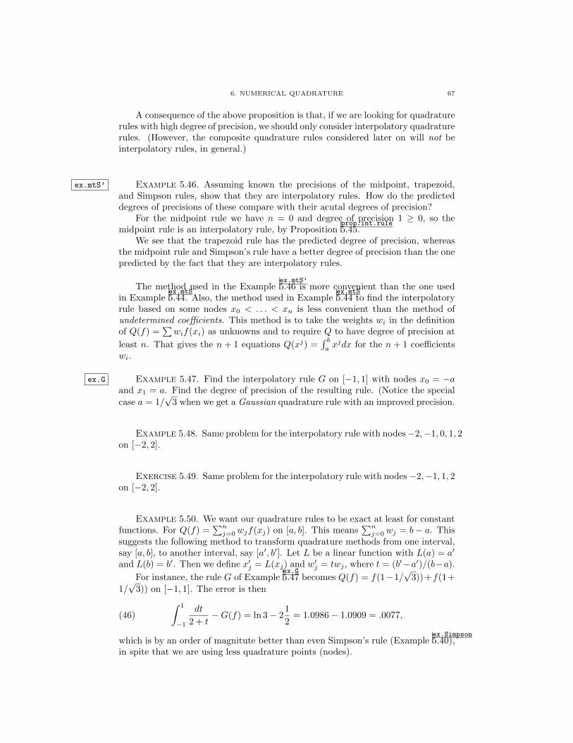
6. NUMERICAL QUADRATURE 67
A consequence of the above proposition is that, if we are looking for quadraturerules with high degree of precision, we should only consider interpolatory quadraturerules. (However, the composite quadrature rules considered later on will not beinterpolatory rules, in general.)
ex.mtS’ Example 5.46. Assuming known the precisions of the midpoint, trapezoid,and Simpson rules, show that they are interpolatory rules. How do the predicteddegrees of precisions of these compare with their acutal degrees of precision?
For the midpoint rule we have n = 0 and degree of precision 1 ≥ 0, so themidpoint rule is an interpolatory rule, by Proposition
prop.int.rule5.45.
We see that the trapezoid rule has the predicted degree of precision, whereasthe midpoint rule and Simpson’s rule have a better degree of precision than the onepredicted by the fact that they are interpolatory rules.
The method used in the Exampleex.mtS’5.46 is more convenient than the one used
in Exampleex.mtS5.44. Also, the method used in Example
ex.mtS5.44 to find the interpolatory
rule based on some nodes x0 < . . . < xn is less convenient than the method ofundetermined coefficients. This method is to take the weights wi in the definitionof Q(f) =
∑wif(xi) as unknowns and to require Q to have degree of precision at
least n. That gives the n + 1 equations Q(xj) =∫ baxjdx for the n + 1 coefficients
wi.
ex.G Example 5.47. Find the interpolatory rule G on [−1, 1] with nodes x0 = −aand x1 = a. Find the degree of precision of the resulting rule. (Notice the special
case a = 1/√
3 when we get a Gaussian quadrature rule with an improved precision.
Example 5.48. Same problem for the interpolatory rule with nodes−2,−1, 0, 1, 2on [−2, 2].
Exercise 5.49. Same problem for the interpolatory rule with nodes−2,−1, 1, 2on [−2, 2].
Example 5.50. We want our quadrature rules to be exact at least for constantfunctions. For Q(f) =
∑nj=0 wjf(xj) on [a, b]. This means
∑nj=0 wj = b− a. This
suggests the following method to transform quadrature methods from one interval,say [a, b], to another interval, say [a′, b′]. Let L be a linear function with L(a) = a′
and L(b) = b′. Then we define x′j = L(xj) and w′j = twj , where t = (b′−a′)/(b−a).
For instance, the rule G of Exampleex.G5.47 becomes Q(f) = f(1−1/
√3))+f(1+
1/√
3)) on [−1, 1]. The error is then
(46)
∫ 1
−1
dt
2 + t−G(f) = ln 3− 2
1
2= 1.0986− 1.0909 = .0077,
which is by an order of magnitute better than even Simpson’s rule (Exampleex.Simpson5.40),
in spite that we are using less quadrature points (nodes).

68 5. NUMERICAL SOLUTION OF NON-LINEAR EQUATIONS
6.3. Error estimates for interpolation rules. The simplest error estimateis obtained from the error estimate in the interpolation formula. We shall use theassumptions and notations of Theorem
thm.interp.error3.7. In particular, x0, x1, . . . , xn ∈ [a, b] are
the nodes and Π(x) = (x− x0)(x− x1) . . . (x− xn).
thm.error.quad Theorem 5.51. Let us assume that |f (n+1)(c)| ≤ Mn+1 and Q is the interpo-latory quadrature rule with nodes x0, x1, . . . , xn ∈ [a, b]. Then∣∣ ∫ b
a
f(t)dt−Q(f)∣∣ ≤ Mn+1
(n+ 1)!
∫ b
a
|Π(x)|dx.
Proof. This follows right away from Theoremthm.interp.error3.7. (Exercise: Check this.) �
Example 5.52. Let Q be the interpolatory rule with n+1 equally spaced nodes
on [a, b]. Write an error estimate for∣∣ ∫ baexdx−Q(ex)
∣∣ using the above theorem.
Exercise 5.53. Do the same for f(x) = cosx.
Improved estimates are possible. In one direction one can get a more precisehold on the constant in from of f (n+1). In another direction, one can replace f (n+1)
with f (k+1), where k is the degree of precision of the rule. For instance, for thethree basic rules that we have discussed (midpoint, trapezoid, Simpson), we havethe following error estimates.
eq.b.quad.errorseq.b.quad.errors (47)
∫ b
a
f(t)dt−Qm(f) =(b− a)3
24f ′′(cm)∫ b
a
f(t)dt−Qt(f) = − (b− a)3
12f ′′(ct)∫ b
a
f(t)dt−Qs(f) = − (b− a)5
2880f (4)(cs).
Example 5.54. Write an error estimate for∫ baf(t)dt − Qm(f) for f(t) = tk,
k = 1, 2, 3.
Exercise 5.55. Same for the other two rules (trapezoid and Simpson).
6.4. Composite rules and error estimates. (Definition of composite rulesfor equally spaced division points. Error estimates for the basic formulas.)
Let us divide the given interval I = [a, b]. We divide I into smaller intervals andthen we approximate the integrals on each of the smaller intervals. The integral onthe bigger interval is then approximated with the sum of the approximations on thesmaller intervals. For instance, let us denote by QI one of our basic interpolationrules (midpoint, trapezoind, Simpson, ... ) on the interval I and decompose I =∪Kk=1Ik into non-overlapping intervals. Then the composite rule is
eq.def.compositeeq.def.composite (48) Qcomposite(f) =
K∑k=1
QIk(f).
The error estimates are obtained from the error estimates on each interval. Letus consider as an example the midpoint rule. In all our examples, we shall divide

6. NUMERICAL QUADRATURE 69
our given interval into m equal subintervals of length h = (b − a)/m. Then thecomposite midpoint rule with m equal intervals is
eq.composite.mideq.composite.mid (49) Qcomposite(f) = h
m∑j=1
f(a+ (j − 1/2)h).
Let us estimate the error using Equation (eq.b.quad.errors47). Then, assuming that |f ′′(t)| ≤ M2
for all t, we have the following important estimate.
eq.def.compositeeq.def.composite (50)∣∣Qcomposite(f)−
∫ b
a
f(t)dt∣∣
≤∣∣∣ m∑j=1
(hf(a+ (j − 1/2)h)−
∫ a+jh
a+(j−1)hf(t)dt
)∣∣∣≤ mh3
24M2 =
(b− a)3
24m2M2 =
(b− a)
24M2h
2 .
This shows that if you double the number of points, then the error becomes aboutfour times smaller. Note that the power 3 in m3 is related to the degree of precision.Using a composite Simpson rule will improve this power to m5.
Exercise 5.56. Carry a similar analysis for the trapezoid and Simpson com-posite rules.
Exercise 5.57. Write an error estimate for the basic composite rules (mid-point, trapezoid, Simpson) for the functions sinx, cosx, ex, and xk.
6.5. Gaussian quadrature. The Gaussian quadrature rules give the bestprecision for quadratures with a fixed number of points. Let us introduce theLegendre polynomials
Ln(x) =[(x2 − 1)n
](n).
Then Ln is a polynomial of degre n with n distinct roots in [−1, 1].
thm.Gaussian.quadr Theorem 5.58. Let x0 < x1 < . . . < xn be the roots of Ln+1, the Legendrepolynomial of degree n+ 1. Let Gn be the quadrature rule on [−1, 1] with the givennodes. Then Gn has degree of precision 2n+ 1.
The rules Gn are called Gaussian quadrature rules. So while the expecteddegree of precision for a rule with n + 1 nodes is n, for the Gaussian quadraturethe achieved precision is 2n+ 1, much higher! For n = 0, the Gaussian quadraturerule is the midpoint rule.
Find the Gaussian quadrature rules G1 and G2 and write an error estimate forthese rules using Theorem
thm.error.quad5.51.
The Legendre polynomials satisfy are orthogonal with respect to the inner
product (f, g) =∫ 1
−1 f(t)g(t)dt:
(51) (Lk, Lj) =
∫ 1
−1Lk(t)Lj(t)dt = 0, if j 6= k.

70 5. NUMERICAL SOLUTION OF NON-LINEAR EQUATIONS
Let qn(x) = Ln/(2nn!). Then
(n+ 1)qn+1(x) = (2n+ 1)xqn(x)− nqn−1(x)
and∫ 1
−1 qn(x)2dx = 2/(2n+ 1).
Exercise 5.59. Write the Legendre polynomials of degree up to 7.
Exercise 5.60. Show that G0(f) = 2f(0), G1(f) = f(−1/√
3) + f(1/√
3),
G3(f) = (5f(−α) + 8f(0) + 5f(α))/9, where α =√
3/5.
Exercise 5.61. Find the interpolatory rule on [−1, 1] with nodes x0 = −α,x1 = 0 and x2 = α. What is its degree of precision?
Exercise 5.62. Find the interpolatory rule Q on [−1, 1] with nodes x0 = −β,x1 = −α, x2 = 0, x3 = α, and x4 = β. What is its degree of precision? Show
that Q(f) = 2(f(−β) + f(−α) + f(0) + f(α) + f(β))/5, if α =√
(5−√
11)/12 and
β =√
(5 +√
11)/12.
7. Numerical Differentiation
We shall now study the approximation of the derivatives of various functions.Let f : [a, b] → R be a function whose derivatives we want to approximate. Weshall denote by Mk the maximum of the function |f (k)| on [a, b], assuming that itexists.
We have the following result.
Theorem 5.63. Assume x, x+ h, x− h ∈ [a, b]. Then
(1)∣∣∣f ′(x)− f(x+h)−f(x)
h
∣∣∣ ≤ hM2/2.
(2)∣∣∣f ′(x)− f(x+h)−f(x−h)
h
∣∣∣ ≤ h2M3/3.
(3)∣∣∣f ′(x)− f(x+h)−2f(x)+f(x−h)
h2
∣∣∣ ≤ h2M4/12.
Proof. This follows from the Taylor’s formula. �