an introduction to stochastic vehicle routing michel gendreau cirrelt and magi École polytechnique...
TRANSCRIPT
An Introduction to Stochastic Vehicle Routing
Michel GendreauCIRRELT and MAGIÉcole Polytechnique de Montréal
PhD course on Local Distribution PlanningMolde University College − March 12-16, 2012
Introduction to Stochastic Vehicle Routing
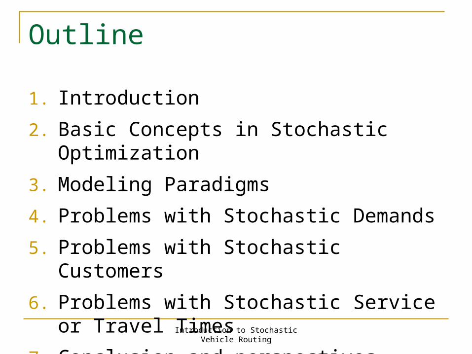
Outline
1. Introduction
2. Basic Concepts in Stochastic Optimization
3. Modeling Paradigms
4. Problems with Stochastic Demands
5. Problems with Stochastic Customers
6. Problems with Stochastic Service or Travel Times
7. Conclusion and perspectives
Introduction to Stochastic Vehicle Routing
Acknowledgements
Walter Rei CIRRELT and ESG UQÀM
Ola Jabali CIRRELT and HEC Montréal
Tom van Woensel and Ton de KokSchool of Industrial EngineeringEindhoven University of Technology
Introduction
Introduction to Stochastic Vehicle Routing
Vehicle Routing Problems
Introduced by Dantzig and Ramser in 1959
One of the most studied problem in the area of logistics
The basic problem involves delivering given quantities of some product to a given set of customers using a fleet of vehicles with limited capacities.
The objective is to determine a set of minimum-cost routes to satisfy customer demands.
Introduction to Stochastic Vehicle Routing
Vehicle Routing Problems
Many variants involving different constraints or parameters:
Introduction of travel and service times with route duration or time window constraints
Multiple depots
Multiple types of vehicles
...
Introduction to Stochastic Vehicle Routing
What is Stochastic Vehicle Routing?Basically, any vehicle routing problem in which one or several of the parameters are not deterministic:
Demands
Travel or service times
Presence of customers
…
Basic Concepts in Stochastic Optimization
Introduction to Stochastic Vehicle Routing
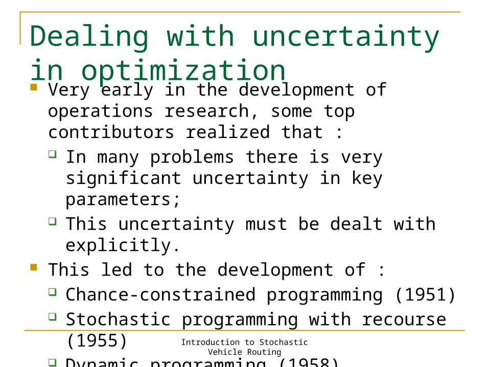
Dealing with uncertainty in optimization Very early in the development of operations
research, some top contributors realized that : In many problems there is very significant
uncertainty in key parameters; This uncertainty must be dealt with explicitly.
This led to the development of : Chance-constrained programming (1951) Stochastic programming with recourse (1955) Dynamic programming (1958) Robust optimization (more recently)
Introduction to Stochastic Vehicle Routing
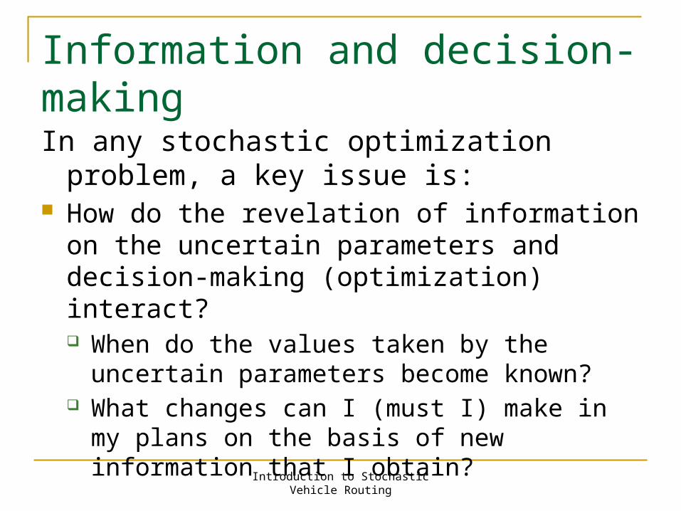
Information and decision-makingIn any stochastic optimization problem, a key
issue is: How do the revelation of information on the
uncertain parameters and decision-making (optimization) interact? When do the values taken by the uncertain
parameters become known? What changes can I (must I) make in my plans on
the basis of new information that I obtain?
Introduction to Stochastic Vehicle Routing
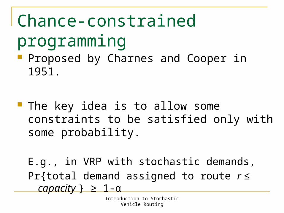
Chance-constrained programming Proposed by Charnes and Cooper in 1951.
The key idea is to allow some constraints to be satisfied only with some probability.
E.g., in VRP with stochastic demands,
Pr{total demand assigned to route r ≤ capacity } ≥ 1-α
Introduction to Stochastic Vehicle Routing
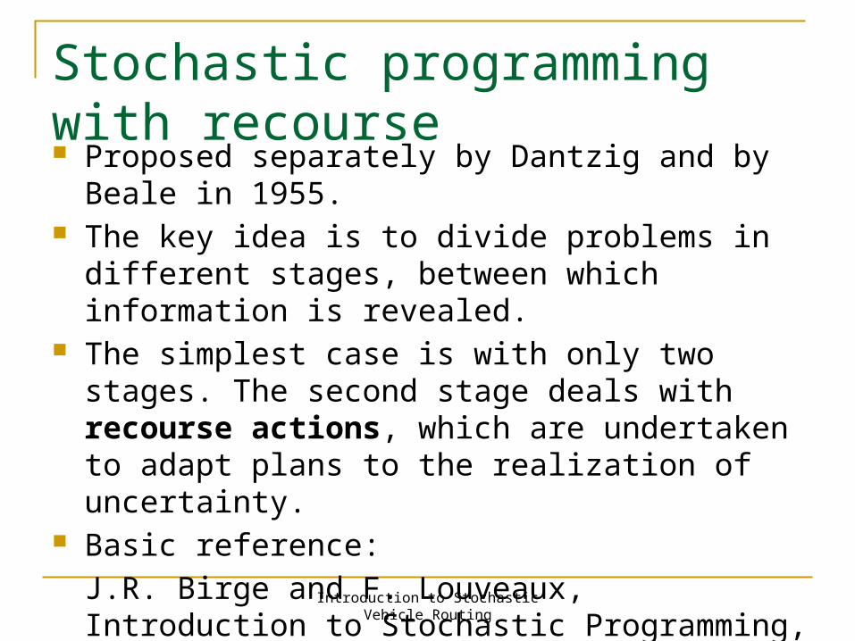
Stochastic programming with recourse Proposed separately by Dantzig and by Beale in
1955. The key idea is to divide problems in different stages,
between which information is revealed. The simplest case is with only two stages. The
second stage deals with recourse actions, which are undertaken to adapt plans to the realization of uncertainty.
Basic reference:
J.R. Birge and F. Louveaux, Introduction to Stochastic Programming, 2nd edition, Springer, 2011.
Introduction to Stochastic Vehicle Routing
Dynamic programming Proposed by Bellman in 1958. A method developed to tackle effectively sequential
decision problems. The solution method relies on a time decomposition
of the problem according to stages. It exploits the so-called Principle of Optimality.
Good for problems with limited number of possible states and actions.
Basic reference:
D.P. Bertsekas, Dynamic Programming and Optimal Control, 3rd edition, Athena Scientific, 2005.
Introduction to Stochastic Vehicle Routing
Here, uncertainty is represented by the fact that the uncertain parameter vector must belong to a given polyhedral set (without any probability defined) E.g., in VRP with stochastic demands,
having set upper and lower bounds for each demand, together with an upper bound on total demand.
Robust optimization looks in a minimax fashion for the solution that provides the best “worst case”.
Robust optimization
Modelling paradigms
Introduction to Stochastic Vehicle Routing
Also called re-optimization Based on the implicit assumption that information
is revealed over time as the vehicles perform their assigned routes.
Relies on Dynamic programming and related approaches (Secomandi et al.)
Routes are created piece by piece on the basis on the information currently available.
Not always practical (e.g., recurrent situations)
Real-time optimization
Introduction to Stochastic Vehicle Routing
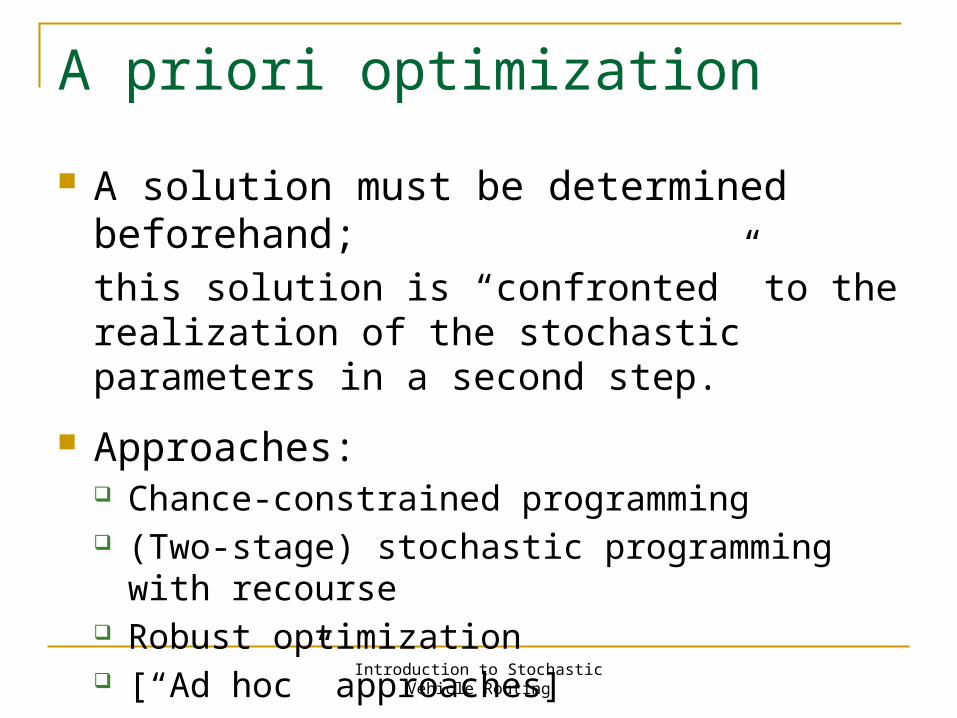
A priori optimization
A solution must be determined beforehand;this solution is “confronted” to the realization of the stochastic parameters in a second step.
Approaches: Chance-constrained programming (Two-stage) stochastic programming with recourse Robust optimization [“Ad hoc” approaches]
Introduction to Stochastic Vehicle Routing
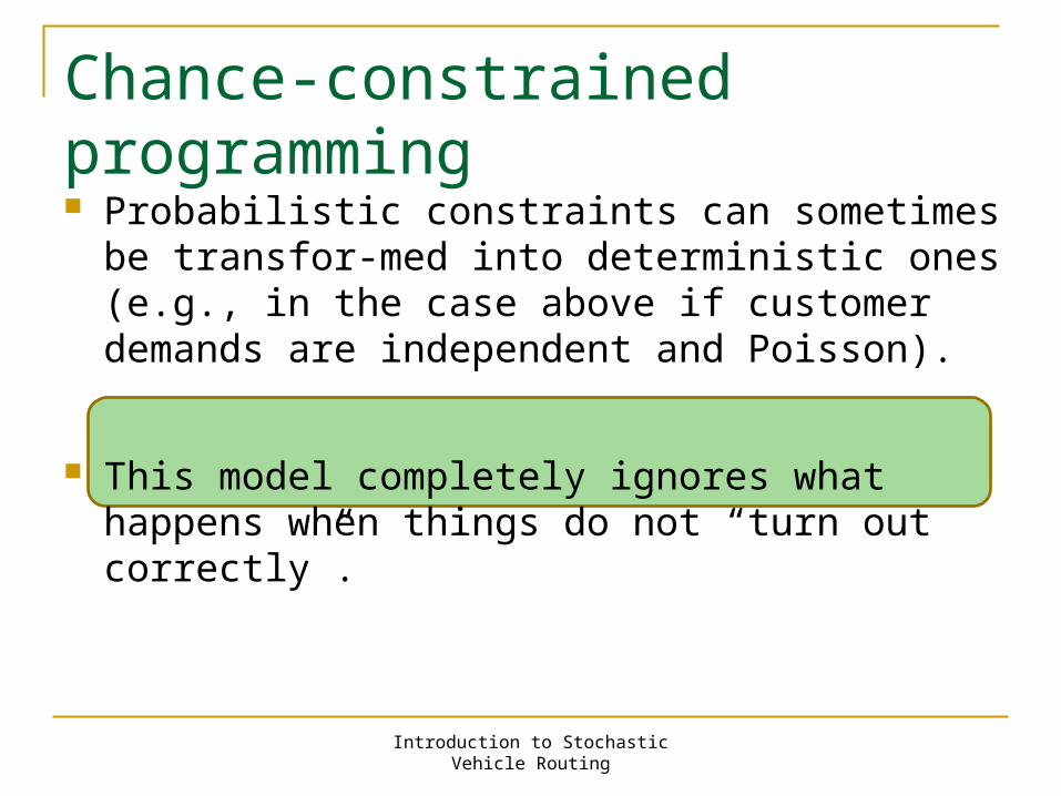
Probabilistic constraints can sometimes be transfor-med into deterministic ones (e.g., in the case above if customer demands are independent and Poisson).
This model completely ignores what happens when things do not “turn out correctly”.
Chance-constrained programming
Introduction to Stochastic Vehicle Routing
Not used very much in stochastic VRP up to now.
Model may be overly pessimistic.
Robust optimization
Introduction to Stochastic Vehicle Routing
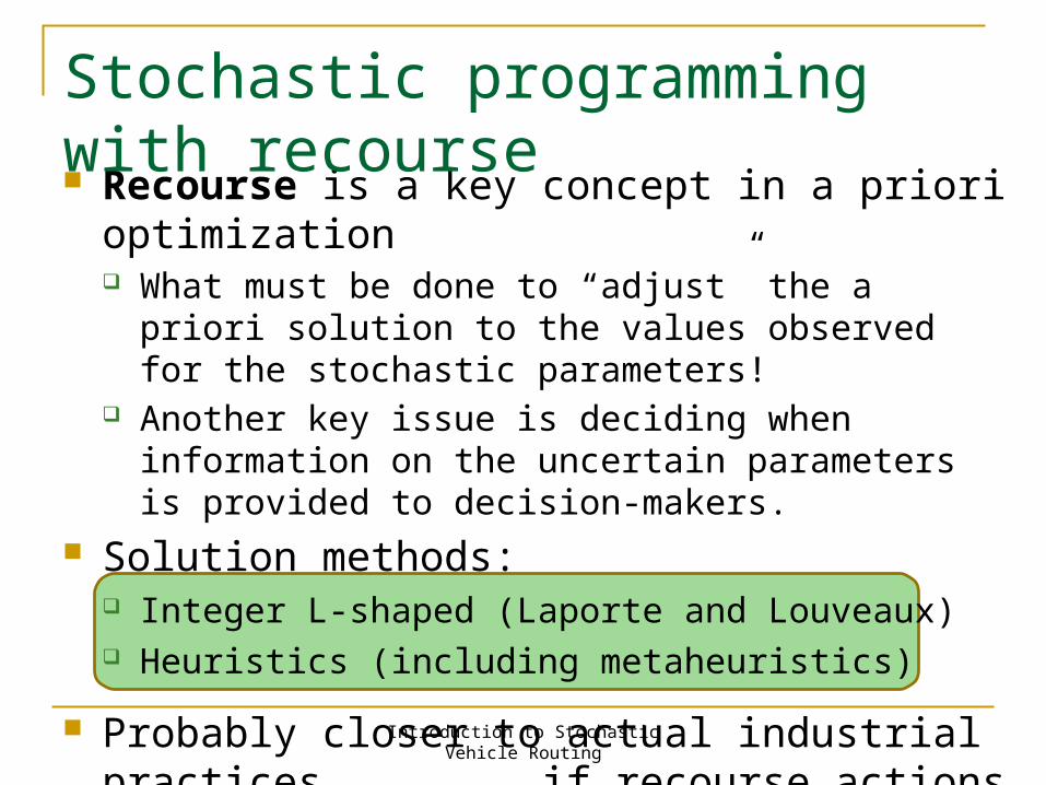
Recourse is a key concept in a priori optimization What must be done to “adjust” the a priori solution to the
values observed for the stochastic parameters! Another key issue is deciding when information on the
uncertain parameters is provided to decision-makers. Solution methods:
Integer L-shaped (Laporte and Louveaux) Heuristics (including metaheuristics)
Probably closer to actual industrial practices, if recourse actions are correctly defined!
Stochastic programming with recourse
VRP with stochastic demands
Introduction to Stochastic Vehicle Routing
A probability distribution is specified for the demand of each customer.
One usually assumes that demands are independent (this may not always be very realistic...).
Probably, the most extensively studied SVRP: Under the reoptimization approach (Secomandi) Under the a priori approach (several authors) using
both the chance-constrained and the recourse models.
VRP with stochastic demands (VRPSD)
Introduction to Stochastic Vehicle Routing
Probably, the most extensively studied SVRP: Under the reoptimization approach (Secomandi et al.) Under the a priori approach (several authors) using both
the chance-constrained and the recourse models. Classical recourse strategy:
Return to depot to restore vehicle capacity Does not always seem very appropriate or “intelligent”
However, recently many authors have started proposing more creative recourse schemes: Pairing routes (Erera et al.) Preventive restocking (Yang, Ballou, and Mathur)
VRP with stochastic demands
Introduction to Stochastic Vehicle Routing
Additional material: M. Gendreau, W. Rei and P. Soriano, “A Hybrid
Monte Carlo Local Branching Algorithm for the Single Vehicle Routing Problem with Stochastic Demands”, presented at GOM 2008, August 2008.
W. Rei and M. Gendreau, “An Exact Algorithm for the Multi-Vehicle Routing Problem with Stochastic Demands”, presented at the TU Eindhoven, November 2009.
VRP with stochastic demands
VRP with stochastic customers
Introduction to Stochastic Vehicle Routing
Each customer has a given probability of requiring a visit.
Problem grounded in the pioneering work of Jaillet (1985) on the Probabilistic Traveling Salesman Problem (PTSP).
At first sight, the VRPSC is of no interest under the reoptimization approach.
VRP with stochastic customers (VPRSC)
Introduction to Stochastic Vehicle Routing
Recourse action: “Skip” absent customers
Has been extensively studied by Gendreau, Laporte and Séguin in the 1990’s: Exact and heuristic solution approaches
Has also been used to model the Consistent VRP (following slides).
VRP with stochastic customers (VPRSC)
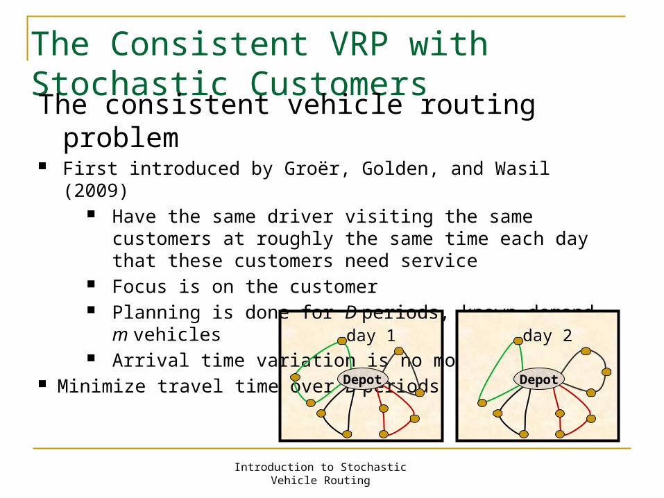
The Consistent VRP with Stochastic CustomersThe consistent vehicle routing problem First introduced by Groër, Golden, and Wasil (2009)
Have the same driver visiting the same customers at roughly the same time each day that these customers need service
Focus is on the customer Planning is done for D periods, known demand, m
vehicles Arrival time variation is no more than L
Minimize travel time over D periods
Introduction to Stochastic Vehicle Routing
day 1 day 2
DepotDepot
Introduction to Stochastic Vehicle Routing
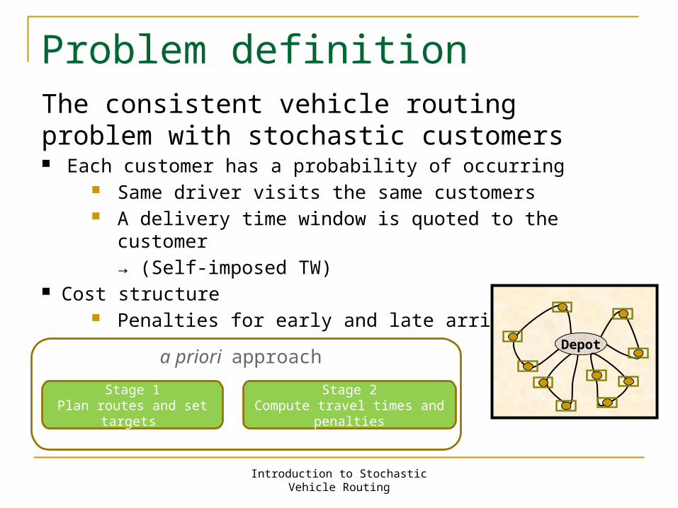
Problem definition The consistent vehicle routing problem with stochastic customers Each customer has a probability of occurring
Same driver visits the same customers A delivery time window is quoted to the customer
→ (Self-imposed TW) Cost structure
Penalties for early and late arrivals Travel times
Depota priori approach
Stage 1Plan routes and set
targets
Stage 2Compute travel times and
penalties
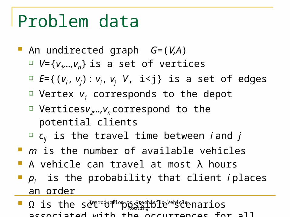
Problem data An undirected graph G=(V,A)
V={v1,..,vn} is a set of vertices E={(vi, vj): vi, vj V, i<j} is a set of edges Vertex v1 corresponds to the depot Verticesv2,..,vn correspond to the potential
clients cij is the travel time between i and j
m is the number of available vehicles A vehicle can travel at most λ hours pi is the probability that client i places an order Ω is the set of possible scenarios associated with
the occurrences for all customersIntroduction to Stochastic Vehicle Routing
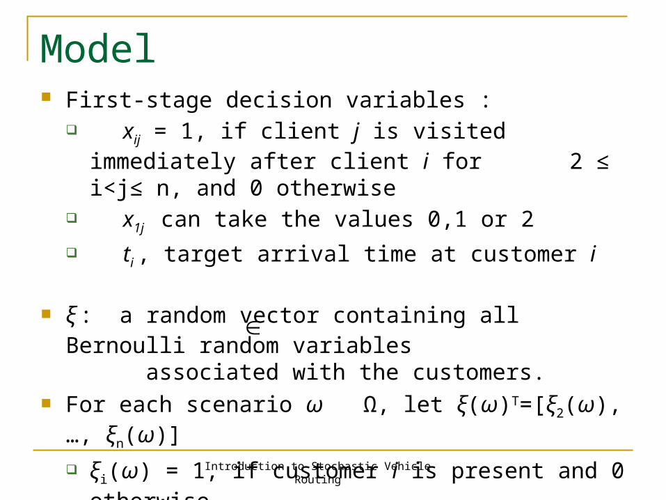
Model First-stage decision variables :
xij = 1, if client j is visited immediately after client i for 2 ≤ i<j≤ n, and 0 otherwise
x1j can take the values 0,1 or 2 ti , target arrival time at customer i
ξ : a random vector containing all Bernoulli random variables associated with the customers.
For each scenario ω Ω, let ξ(ω)T=[ξ2(ω), …, ξn(ω)] ξi(ω) = 1, if customer i is present and 0 otherwise.
Q(x) : second-stage cost (recourse)Introduction to Stochastic Vehicle Routing
Introduction to Stochastic Vehicle Routing
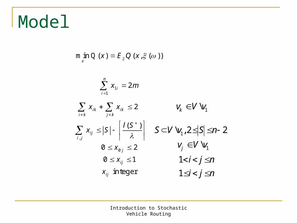
Model
11
,
0
min Q( ) ( , ( ))
2
2
( )
0 2
0 1
integer
x
n
ii
ik iki k j k
ïji j
j
ij
ij
x E Q x
x m
x x
l Sx S
x
x
x
1
1
\ , 2 2
\
1
1
j
S V v S n
v V v
i j n
i j n
1 \
kv V v
Model
T
,min c ( )x t
x Q x
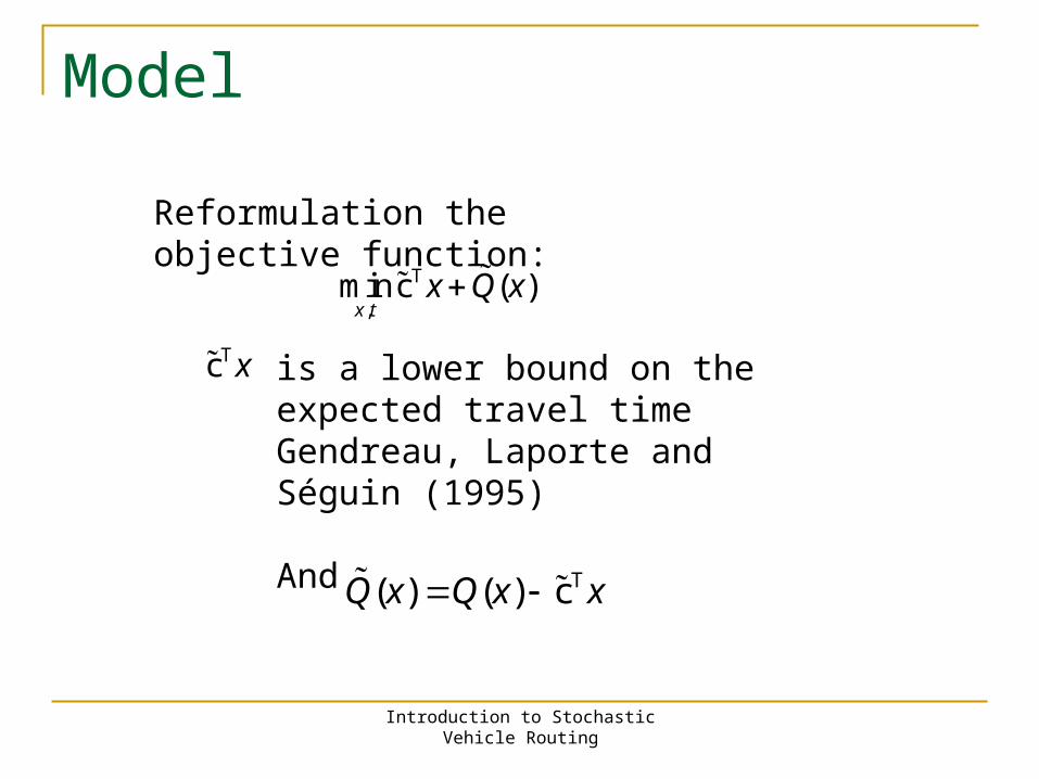
Introduction to Stochastic Vehicle Routing
Tc x
Reformulation the objective function:
is a lower bound on the expected travel timeGendreau, Laporte and Séguin (1995)
And T( ) ( ) cQ x Q x x
Model
Assumption: early arrivals do not wait for the time window
Evaluation of the second stage cost Qr,δ: expected recourse cost corresponding to route r if
orientation δ is chosenQP
r,δ: total average penalties associated with time window deviations for route r if orientation δ is chosen
QTr: total average travel time for route for route r
Introduction to Stochastic Vehicle Routing
, ,r r rT PQ Q Q ,1 ,2
1
( ) min{ , }m
r r
r
Q x Q Q
Model
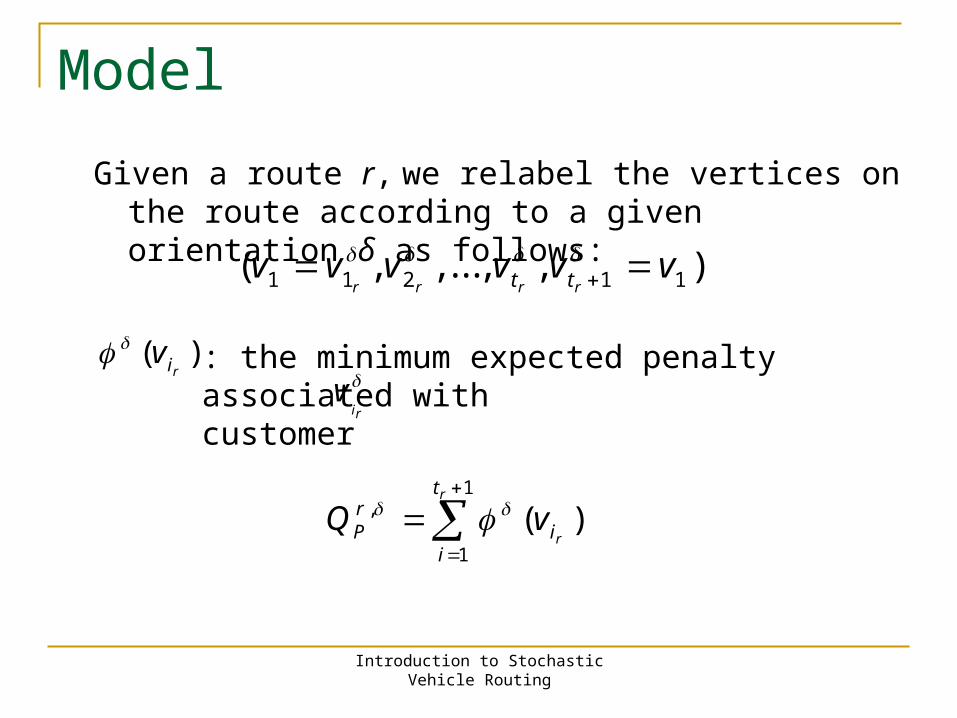
Given a route r, we relabel the vertices on the route according to a given orientation δ as follows:
Introduction to Stochastic Vehicle Routing
1 1 2 1 1( , ,..., , )r r r rt tv v v v v v
( )riv : the minimum expected penalty
associated with customer irv
1,
1
( )r
r
trP i
i
Q v
Introduction to Stochastic Vehicle Routing
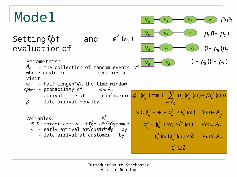
Model( )
riv
v0 v5 v4v7
v0 v5 v4
v0 v4v7
v0 v4
5 7p p
5 7(1 )p p
5 7(1 )p p
5 7(1 )(1 )p p
Setting of and evaluation of
Parameters:– the collection of random events
where customer requires a visitw – half length of the time windowpω – probability of
– arrival time at considering β – late arrival penalty
Variables: – target arrival time at customer– early arrival at customer by – late arrival at customer by
riA riA
riv
rit
rie
ril
( )ria
riv
riv
riv
riv
riA
riA
riA
( ) min ( ( ) ( ))
s.t. [ ] ( )
[ ] ( )
( ), ( ) 0
0
r r r
ir
r r r r
r r r r
r r r
r
i i iA
i i i i
i i i i
i i i
i
v p e l
t w a e A
a t w l A
e l A
t
rit
rit
Introduction to Stochastic Vehicle Routing
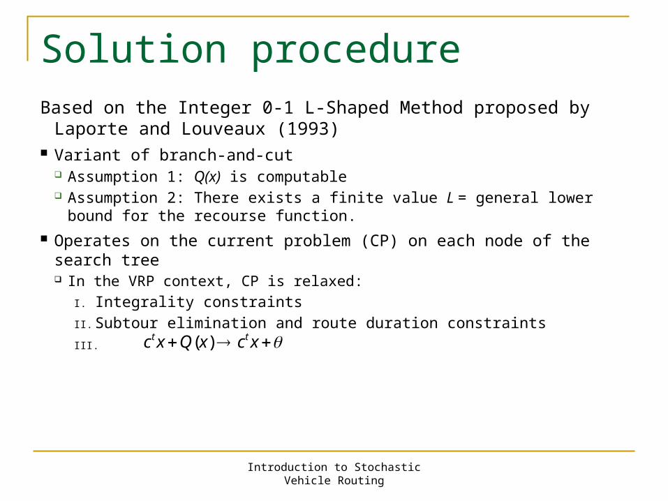
Solution procedureBased on the Integer 0-1 L-Shaped Method proposed by Laporte
and Louveaux (1993) Variant of branch-and-cut
Assumption 1: Q(x) is computable Assumption 2: There exists a finite value L = general lower bound for
the recourse function. Operates on the current problem (CP) on each node of the search
tree In the VRP context, CP is relaxed:
I. Integrality constraints II. Subtour elimination and route duration constraintsIII.
( )t tc x Q x c x
Introduction to Stochastic Vehicle Routing
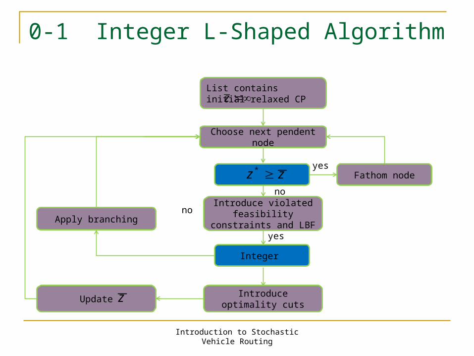
0-1 Integer L-Shaped Algorithm
List contains initial relaxed CP :z
Choose next pendent node
*z z
Integer
Introduce violated feasibility constraints
and LBF
Introduce optimality cuts
Update z
Apply branching
Fathom node
yes
no
no
yes
Introduction to Stochastic Vehicle Routing
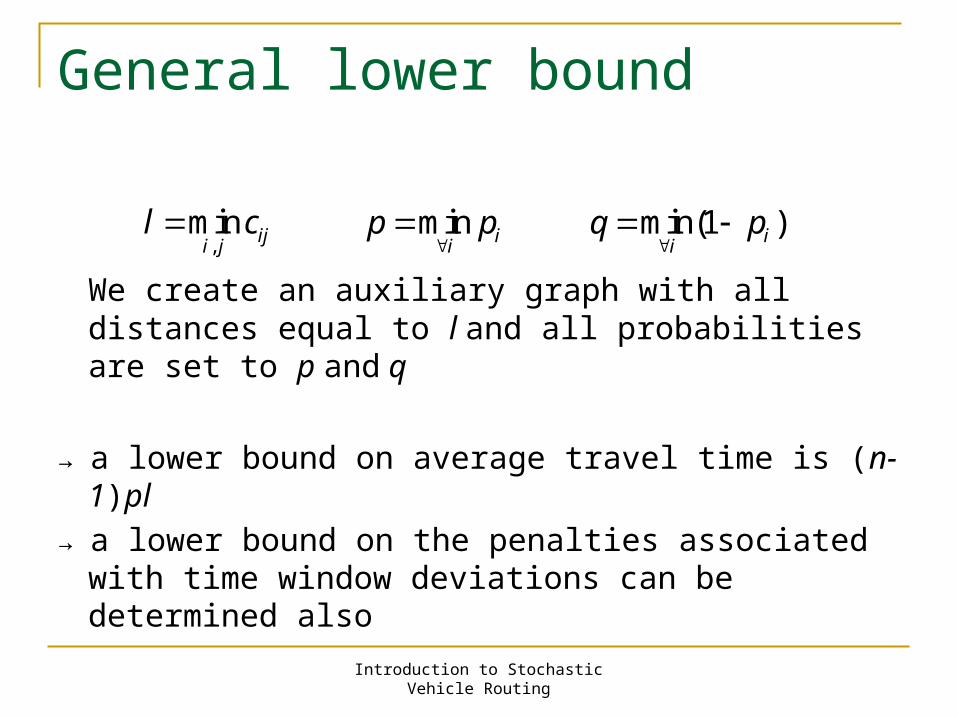
General lower bound
We create an auxiliary graph with all distances equal to l and all probabilities are set to p and q
→ a lower bound on average travel time is (n-1)pl→ a lower bound on the penalties associated with
time window deviations can be determined also
,min iji j
l c min ii
p p
min(1 )ii
q p
v3
v2
v6
{ }
{ }S
T
U S v
U T v
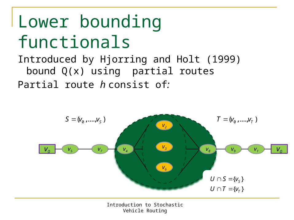
Lower bounding functionals
Introduced by Hjorring and Holt (1999) bound Q(x) using partial routes
Partial route h consist of:
Introduction to Stochastic Vehicle Routing
v0 v5 v4v7
0( ,...., )SS v v
v8 v9 v1 v0
0( ,...., )TT v v
Lower bounding functionals
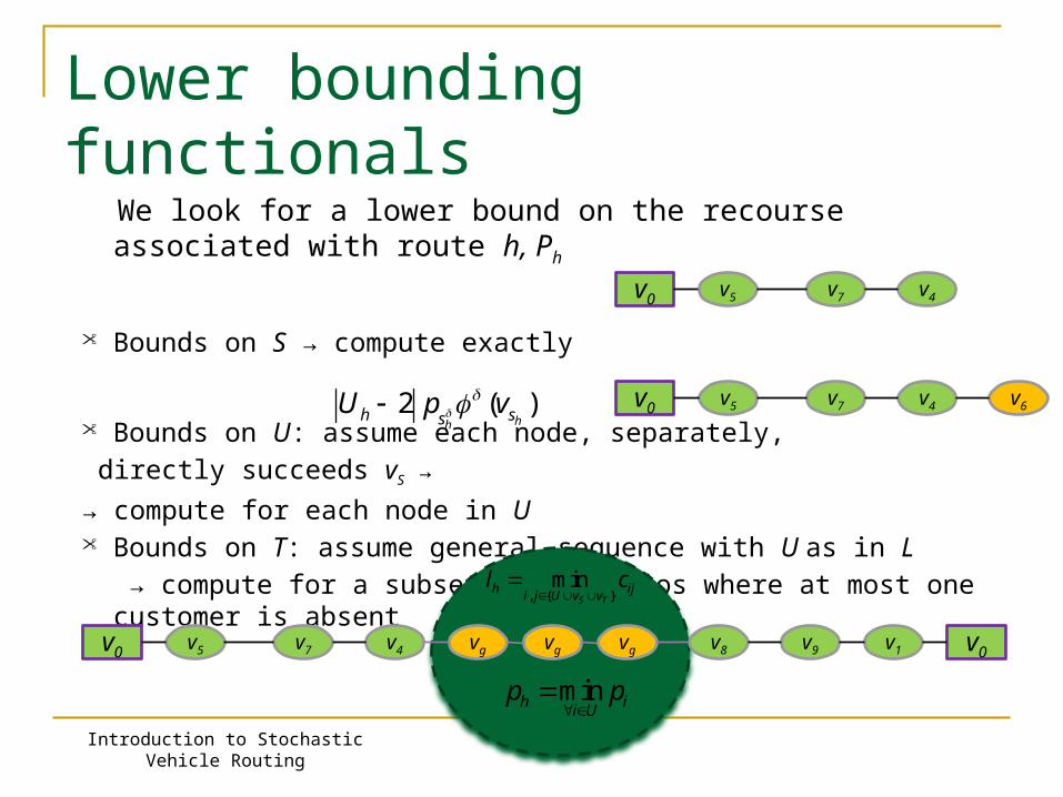
We look for a lower bound on the recourse associated with route h, Ph
• Bounds on S → compute exactly
• Bounds on U: assume each node, separately, directly succeeds vS →
→ compute for each node in U• Bounds on T: assume general sequence with U as in L
→ compute for a subset of scenarios where at most one customer is absent
Introduction to Stochastic Vehicle Routing
v0 v5 v4v7
v0 v5 v4v7 v6
v0 v5 v4v7 v8 v9 v1 v0vg vg vg
, { }min
S Th ij
i j U v vl c
minh ii Up p
2 ( )hh
h ssU p v
Introduction to Stochastic Vehicle Routing
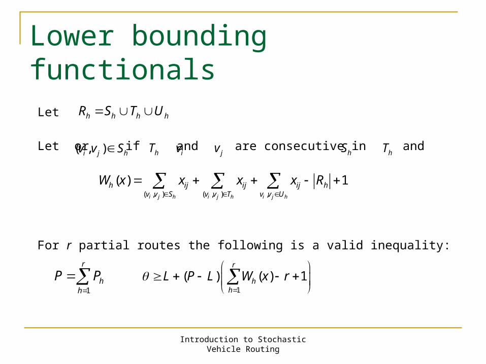
Lower bounding functionals
Let
Let or if and are consecutive in and
For r partial routes the following is a valid inequality:
1
( ) ( ) 1r
hh
L P L W x r
h h h hR S T U
( , ) ( , ) ,
( ) 1i j h i j h i j h
h ij ij ij hv v S v v T v v U
W x x x x R
( , )i j hv v S hT iv jv hS hT
r
hhPP
1
Introduction to Stochastic Vehicle Routing
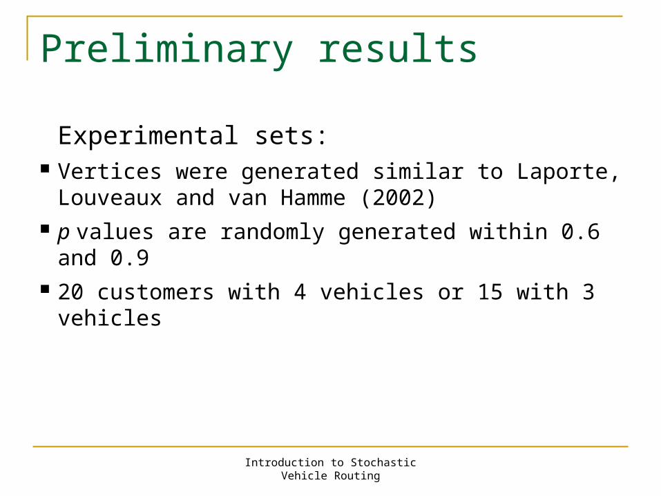
Preliminary results
Experimental sets: Vertices were generated similar to Laporte,
Louveaux and van Hamme (2002) p values are randomly generated within 0.6 and
0.9 20 customers with 4 vehicles or 15 with 3
vehicles
Introduction to Stochastic Vehicle Routing
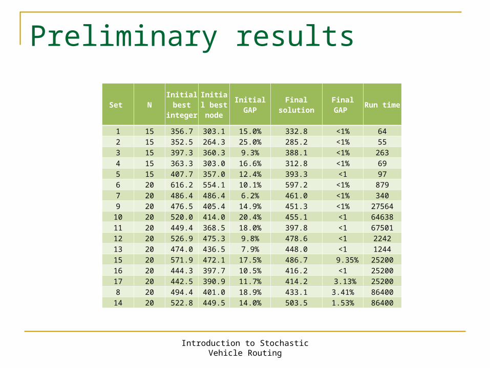
Preliminary results
Set NInitial best
integer
Initial best node
Initial GAP Final solution Final GAP Run time
1 15 356.7 303.1 15.0% 332.8 <1% 642 15 352.5 264.3 25.0% 285.2 <1% 553 15 397.3 360.3 9.3% 388.1 <1% 2634 15 363.3 303.0 16.6% 312.8 <1% 695 15 407.7 357.0 12.4% 393.3 <1 976 20 616.2 554.1 10.1% 597.2 <1% 8797 20 486.4 486.4 6.2% 461.0 <1% 3409 20 476.5 405.4 14.9% 451.3 <1% 27564
10 20 520.0 414.0 20.4% 455.1 <1 6463811 20 449.4 368.5 18.0% 397.8 <1 6750112 20 526.9 475.3 9.8% 478.6 <1 224213 20 474.0 436.5 7.9% 448.0 <1 124415 20 571.9 472.1 17.5% 486.7 9.35% 2520016 20 444.3 397.7 10.5% 416.2 <1 2520017 20 442.5 390.9 11.7% 414.2 3.13% 252008 20 494.4 401.0 18.9% 433.1 3.41% 86400
14 20 522.8 449.5 14.0% 503.5 1.53% 86400
Introduction to Stochastic Vehicle Routing
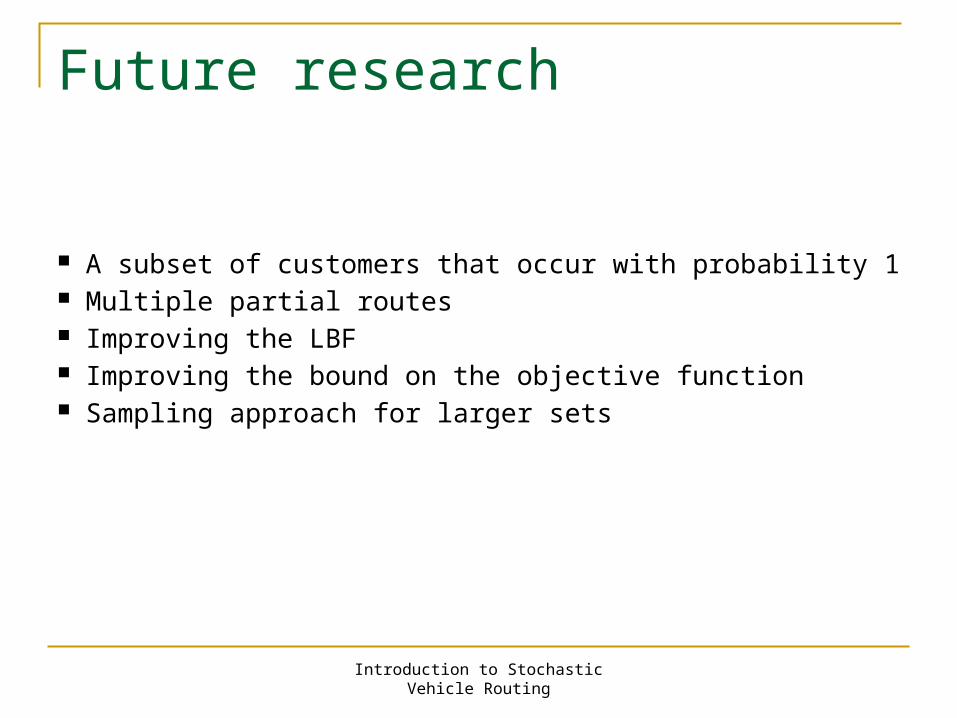
Future research
A subset of customers that occur with probability 1 Multiple partial routes Improving the LBF Improving the bound on the objective function Sampling approach for larger sets
VRP with stochastic service or travel times
Introduction to Stochastic Vehicle Routing
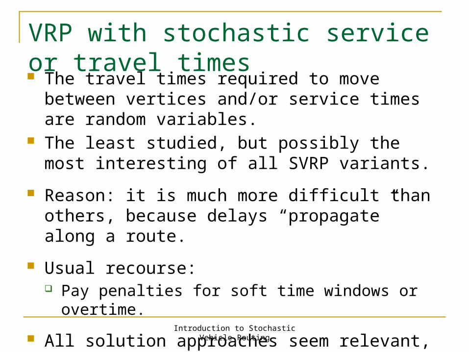
VRP with stochastic service or travel times The travel times required to move between vertices
and/or service times are random variables. The least studied, but possibly the most interesting of
all SVRP variants.
Reason: it is much more difficult than others, because delays “propagate” along a route.
Usual recourse: Pay penalties for soft time windows or overtime.
All solution approaches seem relevant, but present significant implementation challenges.
Conclusions and perspectives
Introduction to Stochastic Vehicle Routing
Conclusion and perspectives Stochastic vehicle routing is a rich and promising
research area. Much work remains to be done in the area of recourse
definition. SVRP models and solution techniques may also be useful
for tackling problems that are not really stochastic, but which exhibit similar structures
Up to now, very little work on problems with stochastic travel and service times, while one may argue that travel or service times are uncertain in most routing problems!
Correlation between uncertain parameters is possibly a major stumbling block in many application areas, but no one seems to work on ways to deal with it.